
1. Introduction
The aim of this paper is to theoretically and numerically investigate the impact of the Hall effect on a magnetohydrodynamic (MHD) dynamo driven in shear flows. The Hall effect is one of the two-fluid effects that are neglected in the usual MHD framework. The effect appears as an additional term in Ohm's law, representing the Hall current induced when the difference in drift motion between ions and electrons occurs. There are many astrophysical and engineering situations where the effect of Hall current must be taken into account. The interstellar medium (Spangler Reference Spangler2001), neutron stars (Goldreich & Reisenegger Reference Goldreich and Reisenegger1992; Shalybkov & Urpin Reference Shalybkov and Urpin1997; Hollerbach & Rüdiger Reference Hollerbach and Rüdiger2002; Gourgouliatos, Hollerbach & Archibald Reference Gourgouliatos, Hollerbach and Archibald2018; Igoshev et al. Reference Igoshev, Hollerbach, Wood and Gourgouliatos2021), ionospheric dynamos (Kelly Reference Kelly2009), solar wind turbulence (Carbone Reference Carbone2012), wave mode conversion in the solar atmosphere (Cally & Khomenko Reference Cally and Khomenko2015; Raboonik & Cally Reference Raboonik and Cally2019), weakly ionised accretion disks (Balbus & Terquem Reference Balbus and Terquem2001; Sano & Stone Reference Sano and Stone2002; Bai Reference Bai2015; Béthune, Lesur & Ferreira Reference Béthune, Lesur and Ferreira2017) are good examples, and the Hall effect is often incorporated in nuclear fusion studies as well (Mahajan & Yoshida Reference Mahajan and Yoshida2000; Hameiri & Ishizawa Reference Hameiri and Ishizawa2005; Hori & Miura Reference Hori and Miura2008). Very recently, a plasma Couette flow experiment has finally become available and interest in the shear-driven Hall-MHD flows has been rapidly increasing (Flanagan et al. Reference Flanagan, Milhone, Egedal, Endrizzi, Olson, Peterson, Sassella and Forest2020; Milhone et al. Reference Milhone, Flanagan, Egedal, Endrizzi, Olson, Peterson, Wright and Forest2021).
The analysis of MHD flows with a Hall term is known to be not easy because it appears as a nonlinear term for the magnetic field in the induction equation. This nonlinear term not only makes it impossible to describe the mechanism of magnetic field generation by linear theory alone but also breaks the symmetry of the MHD equations (see Meyrand & Galtier Reference Meyrand and Galtier2012 for example). From the viewpoint of numerical calculations, this nonlinear term is also troublesome because it excites the high-frequency modes in the magnetic field spectrum (Mininni, Gómez & Mahajan Reference Mininni, Gómez and Mahajan2005; Gómez, Mininni & Dmitruk Reference Gómez, Mininni and Dmitruk2010; Miura & Araki Reference Miura and Araki2014). For these reasons, the properties of Hall-MHD flows are much less understood than those of usual MHD flows, especially in the high-Reynolds-number regime of practical importance.
An MHD dynamo is a state in which a magnetic field is produced by the motion of an electrically conducting fluid alone, without the need for an external magnetic field. Many excellent review papers link various dynamo theories and astrophysical magnetic field generation; see Ossendrijver (Reference Ossendrijver2003), Charbonneau (Reference Charbonneau2014), Rincon (Reference Rincon2019), Tobias (Reference Tobias2021) and references therein. The Hall effect on isotropic dynamos was investigated by Mininni, Gómez & Mahajan (Reference Mininni, Gómez and Mahajan2003); Mininni et al. (Reference Mininni, Gómez and Mahajan2005) using direct numerical simulations of Hall-MHD equations in a periodic cube with a stationary helical kinematic forcing. Their main conclusion was that when the forcing length scale and the Hall length scale (i.e. ion skin depth) are comparable, the dynamo is enhanced but when the latter scale is larger than the former scale, the magnetic field generation is inhibited. Mininni et al. (Reference Mininni, Gómez and Mahajan2003, Reference Mininni, Gómez and Mahajan2005) referred to their dynamos as a large-scale dynamo in the sense that the scale of the generated magnetic field is larger than the energy-containing scale of turbulent eddies. Gómez et al. (Reference Gómez, Mininni and Dmitruk2010) used a random non-helical forcing to study small-scale dynamos and concluded similar results to Mininni et al. (Reference Mininni, Gómez and Mahajan2003, Reference Mininni, Gómez and Mahajan2005). The results that the dynamos are suppressed when the Hall effect is too strong is consistent with that deduced in the pioneering study by Helmis (Reference Helmis1971), who used the mean-field theory.
The subject of our interest in this paper is a dynamo mechanism associated with the spontaneous generation of coherent structures in shear flows. The dynamo driven by a homogeneous shear has been an active area of research in the past decade (Yousef et al. Reference Yousef, Heinemann, Schekochihin, Kleeorin, Rogachevskii, Iskakov, Cowley and McWilliams2008; Tobias & Cattaneo Reference Tobias and Cattaneo2013; Nauman & Blackman Reference Nauman and Blackman2017; Teed & Proctor Reference Teed and Proctor2017; Herreman Reference Herreman2018; Deguchi Reference Deguchi2019a,Reference Deguchib). Since the coherent structures in shear flows are strongly anisotropic and include multiple length scales, it is expected that the impact of the Hall effect on the associated dynamo will be more complex than that seen in the isotropic cases. However, to the best of the author's knowledge, there are no studies that have investigated the Hall effect on shear-driven dynamos.
Our primal goal is to extend the work by Deguchi (Reference Deguchi2019a,Reference Deguchib) who studied exact coherent structures in purely MHD plane Couette flow. The exact coherent structures are unstable three-dimensional nonlinear invariant solutions that mimic the structure of coherent structures in turbulence (Nagata Reference Nagata1990; Clever & Busse Reference Clever and Busse1992; Waleffe Reference Waleffe2001). Although unstable solutions might seem to be physically unimportant at first glance, they are in fact known to play crucial roles in the dynamical systems theory view of turbulence. Studying the solutions has now become popular among hydrodynamicists, rapidly advancing our understanding of the subcritical transition problem (Hof et al. Reference Hof, van Doorne, Westerweel, Nieuwstadt, Faisst, Eckhardt, Wedin, Kerswell and Waleffe2004; Gibson, Halcrow & Cvitanovic Reference Gibson, Halcrow and Cvitanovic2008; Kawahara, Uhlmann & van Veen Reference Kawahara, Uhlmann and van Veen2012). Here the subcritical transition refers to transition routes carved out without the aid of linear instability, which commonly appears in shear flows. Exact coherent structures appear naturally when one tries to find the threshold perturbation amplitude at which the transition occurs (Itano & Toh Reference Itano and Toh2001; Skufca, Yorke & Eckhardt Reference Skufca, Yorke and Eckhardt2006; Wang, Gibson & Waleffe Reference Wang, Gibson and Waleffe2007).
Surprisingly, some solutions allow us to take their infinite-Reynolds-number limit through the matched asymptotic expansion analyses (Hall & Sherwin Reference Hall and Sherwin2010; Deguchi & Hall Reference Deguchi and Hall2014a,Reference Deguchi and Hallb; Deguchi Reference Deguchi2015; Dempsey et al. Reference Dempsey, Deguchi, Hall and Walton2016). Of course, the reason why rational asymptotic analysis is possible is that the solutions possess a much simpler structure than turbulence. Having said that, in recent years some extensions of these theories have been found to be capable of describing more complex and realistic flows. In the latest studies, the qualitative properties of near-wall turbulence were reproduced to some extent by using multiple-scale waves coexisting and interacting through the mean flow (Hall Reference Hall2018; Blackburn, Deguchi & Hall Reference Blackburn, Deguchi and Hall2021). The basis of this multiple-scale state was the fact that the coherent structure can be sustained at any local station of the flow, independent of the presence of walls (Blackburn, Hall & Sherwin Reference Blackburn, Hall and Sherwin2013; Deguchi Reference Deguchi2015). Similar localised coherent structures were also used to build nonlinear structures in various non-parallel flows such as boundary layer flows (Deguchi & Hall Reference Deguchi and Hall2015, Reference Deguchi and Hall2017) and jet flows (Deguchi & Hall Reference Deguchi and Hall2018).
The extension of the above hydrodynamic results to MHD flows is an interesting problem, as subcritical dynamos might be important in some astrophysical flows. The similarity between the shear-driven MHD dynamo problem and the self-sustaining process of hydrodynamic coherent structures (Hall & Smith Reference Hall and Smith1991; Waleffe Reference Waleffe1997) has been repeatedly pointed out (Rincon, Ogilvie & Proctor Reference Rincon, Ogilvie and Proctor2007; Riols et al. Reference Riols, Rincon, Cossu, Lesur, Longaretti, Ogilvie and Herault2013; Herreman Reference Herreman2018; Deguchi Reference Deguchi2019a,Reference Deguchib). Deguchi (Reference Deguchi2019a) recently developed a high-Reynolds-number asymptotic dynamo theory by combining the vortex-wave interaction theory by Hall & Smith (Reference Hall and Smith1991) and the resonant absorption theory for Alfven waves (Sakurai, Goossens & Hollweg Reference Sakurai, Goossens and Hollweg1991; Goossens, Ruderman & Hollweg Reference Goossens, Ruderman and Hollweg1995). Interestingly, the theory covers the limit of large magnetic Reynolds number, which is known to be very important in explaining the generation of magnetic fields in various celestial bodies. Deguchi (Reference Deguchi2019b) then confirmed that the dynamo's exact coherent structures in plane Couette flow indeed obey the asymptotic theory.
This paper is organised as follows. In the next section, we begin by briefly formulating our problem. Section 3 is devoted to the numerical analysis of Hall-MHD dynamo solutions in plane Couette flow at moderately high Reynolds numbers. We begin our analysis from the solutions found in Deguchi (Reference Deguchi2019b) to study the impact of the Hall effect on the magnetic field generation for both moderate and asymptotically large Hall parameters. In § 4 we study the large hydrodynamic/magnetic Reynolds number limit of the solutions using matched asymptotic expansion. We first derive the asymptotic properties of the plane Couette solution found in the previous section, and then show how to extend this result to more general flows. In the former part, we will discuss how to incorporate the Hall effect into the theory by Deguchi (Reference Deguchi2019a). One of the natural questions is: what would be the conditions under which the Hall effect can be neglected? Note here that, because the scaling is strongly anisotropic, it is not obvious how the Hall term affects the high-Reynolds-number dynamo. The latter part is much motivated by the aforementioned hydrodynamic results Deguchi & Hall (Reference Deguchi and Hall2014b) and Blackburn et al. (Reference Blackburn, Deguchi and Hall2021). Finally, we summarise our findings in § 5.
2. Formulation of the problem
Consider the incompressible viscous resistive Hall-MHD equations in the Cartesian coordinates  $(x_*,y_*,z_*)$. In Gaussian units, the evolution equations for the fluid velocity
 $\boldsymbol {v}_*=(u_*,v_*,w_*)$, the total pressure
 $q_*$ and the magnetic field
 $\boldsymbol {b}_*=(a_*,b_*,c_*)$ are written by
 \begin{gather} (\partial_{t_*}+\boldsymbol{v}_*\boldsymbol{\cdot} \boldsymbol{\nabla}_*)\boldsymbol{v}_* -\frac{1}{c_l \rho} (\boldsymbol{b}_*\boldsymbol{\cdot} \boldsymbol{\nabla}_*)\boldsymbol{b}_* ={-}\frac{1}{\rho}\boldsymbol{\nabla}_* q_* + \nu \nabla_*^2 \boldsymbol{v}_*, \end{gather}
 \begin{gather}\partial_{t_*}\boldsymbol{b}_* = \boldsymbol{\nabla}_* \times \left[\left(\boldsymbol{v}_*-\frac{1}{q_e n_e}\boldsymbol{J}_*\right)\times \boldsymbol{b}_*- \frac{4{\rm \pi} \eta}{c_l}\boldsymbol{J}_*\right], \end{gather}
 \begin{gather}\boldsymbol{\nabla}_* \boldsymbol{\cdot} \boldsymbol{v}_* =0,\quad \boldsymbol{\nabla}_* \boldsymbol{\cdot} \boldsymbol{b}_*=0, \end{gather}
where  $\boldsymbol {\nabla }_*=(\partial _{x_*},\partial _{y_*},\partial _{z_*})$,
 $\rho$ is the density,
 $\nu$ is the kinematic viscosity,
 $c_l$ is the speed of light,
 $q_e$ is the electron charge,
 $n_e$ is the number density of electrons. The magnetic diffusivity is defined by
 $\eta ={c_l^2}/{4{\rm \pi} \sigma _c}$ using the electrical conductivity
 $\sigma _c$. The current density is
 $\boldsymbol {J}_*=({c_l}/{4{\rm \pi} })(\boldsymbol {\nabla }_* \times \boldsymbol {b}_*)$.
For definiteness, in the majority of the paper, we study the dynamos in plane Couette flow, where the no-slip and perfectly insulating walls at  $y_*=\pm L_*$ are moving with a speed
 $\pm U_*$ in the
 $x_*$ direction. There is no external magnetic field considered and, hence, the movement of the walls is the only energy input mechanism. The rescaling
 \begin{gather} \boldsymbol{v}_*=U_* \boldsymbol{v}, \quad \boldsymbol{b}_*=\sqrt{c_l\rho}U_*\boldsymbol{b}, \quad q_*=\rho U_*^2 q, \end{gather}
 \begin{gather}(x_*,y_*,z_*)=L_*(x,y,z),\quad \boldsymbol{\nabla}_*=L_*^{{-}1}\boldsymbol{\nabla}, \quad t_*=(L_*/U_*)t, \end{gather}
yields the non-dimensionalised system
 \begin{gather} (\partial_t+\boldsymbol{v}\boldsymbol{\cdot} \boldsymbol{\nabla})\boldsymbol{v} - (\boldsymbol{b}\boldsymbol{\cdot} \boldsymbol{\nabla})\boldsymbol{b} ={-}\boldsymbol{\nabla} q + \frac{1}{R} \nabla^2 \boldsymbol{v}, \end{gather}
 \begin{gather}\partial_t\boldsymbol{b} = \boldsymbol{\nabla} \times [(\boldsymbol{v}-H\boldsymbol{\nabla} \times \boldsymbol{b})\times \boldsymbol{b}]+\frac{1}{R P_m} \nabla^2 \boldsymbol{b}, \end{gather}
 \begin{gather}\boldsymbol{\nabla} \boldsymbol{\cdot} \boldsymbol{v} =0,\quad \boldsymbol{\nabla} \boldsymbol{\cdot} \boldsymbol{b}=0, \end{gather}
where the Reynolds number  $R$, the magnetic Prandtl number
 $P_m$ and the non-dimensional Hall coefficient
 $H$ are defined as
 \begin{equation} R=\frac{U_* L_*}{\nu},\quad P_m=\frac{\nu}{\eta},\quad H=\frac{c_l^{3/2}\rho^{1/2}}{4{\rm \pi} q_e n_e L_*}. \end{equation}
Note that after multiplying  $L_*$, the parameters
 $H$,
 $R^{-1}$ and
 $R^{-1}P_m^{-1}$ become the Hall length, the viscous diffusion length and the Ohmic dissipation length, respectively. Equations (2.5a)–(2.5c) are to be solved with the boundary conditions
 \begin{gather} \boldsymbol{v}=({\pm} 1,0,0), \quad \boldsymbol{b}=\boldsymbol{\nabla} \varphi_{{\pm}}\quad \text{at} \ y={\pm} 1, \end{gather}
 \begin{gather}{}[\boldsymbol{v},\boldsymbol{b}](x,y,z,t)=[\boldsymbol{v},\boldsymbol{b}](x+L_x,y,z,t)=[\boldsymbol{v},\boldsymbol{b}](x,y,z+L_z,t), \end{gather}
where the outer magnetic potential  $\varphi _{\pm }(x,y,z)$ satisfies
 $\nabla ^2 \varphi _{\pm }=0$ with
 $\varphi _{\pm }\rightarrow 0$ as
 $y\rightarrow \pm \infty$.
It is important to note here that there is no forcing term in (2.5a), although in many other shear dynamo studies the momentum equations are supported by an additional small-scale forcing (e.g. Yousef et al. Reference Yousef, Heinemann, Schekochihin, Kleeorin, Rogachevskii, Iskakov, Cowley and McWilliams2008; Tobias & Cattaneo Reference Tobias and Cattaneo2013; Teed & Proctor Reference Teed and Proctor2017; Herreman Reference Herreman2018). In the case there is no external force, the emergence of the dynamo should be understood as a subcritical transition phenomenon, as the base field is linearly stable. The study of such a dynamo has started only recently by the direct numerical simulation (Nauman & Blackman Reference Nauman and Blackman2017) and the exact coherent structures (Deguchi Reference Deguchi2019a,Reference Deguchib).
The laminar Couette flow  $\boldsymbol {v}=(y,0,0), \boldsymbol {b}=(0,0,0)$ is the only possible solution when
 $R$ is small enough, while with increasing
 $R$ a myriad of non-trivial solutions emerge. In this paper we will focus only on the travelling wave solutions, and denote their phase speeds in the
 $x$ and
 $z$ directions as
 $s_x$ and
 $s_z$, respectively.
For each nonlinear solution, the streamwise mean field  $\bar {B}_x(y)$ and the spanwise mean field
 $\bar {B}_z(y)$ can be found from
 \begin{equation} \frac{1}{L_x L_z} \int^{L_x}_0 \int^{L_z}_0 \boldsymbol{b}\,\textrm{d}\kern0.06em x\,\textrm{d}z =[\bar{B}_x,0,\bar{B}_z]. \end{equation}
In order to draw the bifurcation diagrams, we use the mean current on the lower wall
 \begin{equation} \left. \left(\frac{1}{L_x L_z} \int^{L_x}_0 \int^{L_z}_0 (\boldsymbol{\nabla} \times \boldsymbol{b})\,{\textrm{d}\kern0.06em x}\,\textrm{d}z \right)\right|_{y={-}1}= [I_z, 0, -I_x], \end{equation}
where
 \begin{equation} I_x=\left. \frac{\textrm{d}\bar{B}_x}{\textrm{d}y} \right|_{y={-}1},\quad I_z=\left. \frac{\textrm{d}\bar{B}_z}{\textrm{d}y} \right|_{y={-}1}. \end{equation}
3. Results for moderate Reynolds numbers
We first note that the base flow is always linearly stable and, hence, we cannot use the usual bifurcation analysis to find nonlinear solutions. Hence, we instead continue the dynamo solution branch found by Deguchi (Reference Deguchi2019b) for purely MHD Couette flows to the Hall-MHD regime. Of the two solutions produced by the saddle-node bifurcation, we focus on the less energetic one which is often called the lower branch solution. This type of solution is particularly important in discussing subcritical transitions because in the phase space it typically sits at the edge of the basin of attraction of turbulence. Throughout this section, we employ the parameters  $R=1000, P_m=1$ and the box size
 $L_x=2{\rm \pi}, L_z={\rm \pi}$ used in Deguchi (Reference Deguchi2019b). Unstable travelling wave solutions are captured by running Newton's method to the spectrally discretised version of (2.5) from a reasonably good initial guess. The numerical code is based on the Chebyshev–Fourier spectral code by Deguchi (Reference Deguchi2019b). Up to 54th Chebyshev modes are used in the wall-normal direction, and up to 7th and 15th Fourier harmonics are used in the
 $x$ and
 $z$ directions, respectively.
The bifurcation diagrams obtained are summarised in figure 1. The quantity  $I_z$ defined in (2.11a,b) is used in this diagram because it is sensitive to changes in the symmetry of the magnetic field, as we shall see shortly. The starting point of the continuation is point A in figure 1(a) and it corresponds to the MHD dynamo solution (
 $H=0$) by Deguchi (Reference Deguchi2019b). Note that this point is on the red solid branch, and increasing
 $H$ along the branch points B and C are successively obtained. At point C, the red solid branch connects to the green dashed branch, which can be further continued into large and small
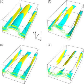
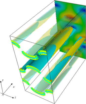
 $H$ regimes. The structures of the solutions at points A, B and C are shown in figure 2(a–c), using the isosurfaces of the streamwise current; in this section we apply a Galilean transformation to make the travelling wave steady, by redefining the
 $x$,
 $z$ coordinates. Those pictures clearly show that the appearance of current sheets characterises the structure of the nonlinear solutions, and moreover, they have a different spatial symmetry at each reference point on the solution branch.
The bifurcation diagram changing the non-dimensional Hall parameter  $H$. The variation of
 $I_z$ is monitored (see (2.11a,b) for definition). The Reynolds number is fixed at
 $R=1000$. Panels (a–d) show the same result, but differ in which part of the solution branch they are focusing on. (a) Point A corresponds to the MHD dynamo solution found in Deguchi (Reference Deguchi2019b). The continuation study began from this point. In the figure, all points A, B, C are on the red solid curve. The solutions on the red and green branches have distinct symmetries. (b) The figure showing that the bifurcation diagram is point symmetric with respect to the origin. The blue dotted branch is the symmetric counterpart of the green dashed branch (this was omitted in figure (a) for the sake of simplicity). The large
 $H$ behaviour of the green and blue branches are studied in (c,d), respectively (irrelevant branches are omitted). In those figures, the black curves represent the large
 $H$ asymptotic solutions.

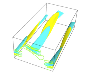
The yellow and blue surfaces are isosurfaces of 50 % magnitude of the positive and negative streamwise current. The isocontours of the current are also shown at the front of the box. The box size is  $[0,2{\rm \pi} ] \times [-1,1] \times [0,{\rm \pi} ]$. Panels (a–c) correspond to A, B and C in figure 1(a), respectively. Panel (d) is the solution at
 $H=0$ but on the green dashed branch in figure 1.

In order to analyse the symmetry, following Gibson et al. (Reference Gibson, Halcrow and Cvitanovic2008), here we use the reflection operators
 \begin{gather} \sigma_{xy} [u,v,w,a,b,c](x,y,z)=[{-}u,-v,w,-a,-b,c]({-}x,-y,z), \end{gather}
 \begin{gather}\sigma_{z} [u,v,w,a,b,c](x,y,z)=[u,v,-w,a,b,-c](x,y,-z), \end{gather}
and the half-shift operators
 \begin{gather} \tau_{x} [u,v,w,a,b,c](x,y,z)=[u,v,w,a,b,c](x+L_x/2,y,z), \end{gather}
 \begin{gather}\tau_{z} [u,v,w,a,b,c](x,y,z)=[u,v,w,a,b,c](x,y,z+L_z/2). \end{gather}
In addition, we consider the operator
 \begin{equation} \gamma [u,v,w,a,b,c](x,y,z)=[u,v,w,-a,-b,-c](x,y,z) \end{equation}
which corresponds to the flip of the polarity.
First, we analyse the symmetry of the system (i.e. the governing equations and the boundary conditions). When  $H=0$, namely for the pure MHD case, it is easy to show that our system is invariant under
 $\sigma _z, \sigma _{xy},\gamma$ and their arbitrary combinations. However, for
 $H\neq 0$, the system is only invariant under
 $\gamma \sigma _z, \sigma _{xy}$ and their combinations. The symmetry breaking with respect to
 $\gamma$ reflects the fact that the difference between the motion of electrons and ions is taken into account in the Hall-MHD equations.
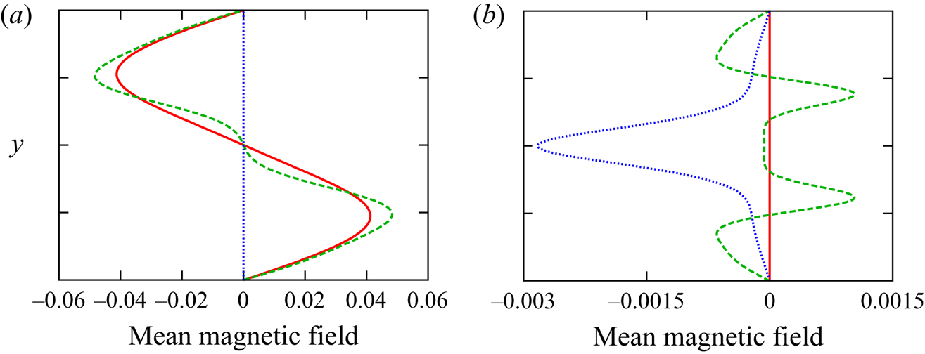
This change in the symmetry of the system of course affects the symmetry of the solutions. Importantly, the symmetries of the flow field have a great impact on the structure of the mean magnetic field as shown in figure 3. Note that what the symmetries of the solution imply for the structure of the mean field is easily seen by examining the  $x$–
 $z$ averaged equations, as summarised in table 1. The properties of the solutions at the reference points are as follows.
(i) The solution at point A computed at
 $H=0$ has invariances against $\tau _x\sigma _z$, $\tau _z\sigma _{xy}$ and the combination of those two. The current sheet seen in figure 2(a) creates a wavy pattern in the $y$–$z$ plane due to the symmetries. Because of the invariances under $\sigma _{xy}$ and $\sigma _z$, the solution is stationary ($s_x=s_z=0$). Table 1 implies that $\bar {B}_z(y)=0$, and $\bar {B}_x(y)$ is an odd function. This is certainly consistent with the mean field shown by the red curves in figure 3.
(ii) The solution at point B is invariant for
$\tau _z\sigma _{xy}$ but not for $\sigma _z$, because as remarked earlier the existence of the Hall effect destroys the latter symmetry. The symmetry breaking is in fact evident in figure 2(b). The flow field travels in the spanwise direction due to the non-zero phase speed $s_z$ produced by the absence of the $\sigma _z$ invariance. Moreover, the spanwise mean magnetic field is generated; $\bar {B}_x$ and $\bar {B}_z$ are odd and even functions, respectively, as shown by the green curves in figure 3 and table 1.(iii) At point C, the solution becomes steady again. This change of the property of the solution is due to the invariance to
$\gamma \sigma _z$ that holds along the green solution branch. The recovery of some symmetry in $z$ at this point can also be seen in the three-dimensional picture in figure 2(c). This symmetry has a different effect on the mean flow than what we saw at point A; see the dotted blue curves in figure 3 where we can confirm the vanishing of the streamwise magnetic field.


The  $x$–
 $z$ average component of the magnetic field generated by the dynamo solutions. In (a) the
 $x$ component of the averaged field
 $\bar {B}_x(y)$ is plotted, while in (b) the
 $z$ component
 $\bar {B}_z(y)$ is used. The red solid, green dashed and blue dotted curves correspond to the solutions at points A, B and C in figure 1(a), respectively.

The required properties for the  $x$–
 $z$ averaged magnetic field when the solution is invariant under the corresponding operators.

The green branch can be continued back to the usual MHD limit  $H=0$; see figure 2(d) for the corresponding flow field. The invariance for
 $\sigma _z$ is still broken even at pure MHD, implying that there are two solutions that transform into each other under this operation. Tracing the branches from the transformed solution we can find the blue dotted curve shown in figure 1(b). As seen in this figure, the bifurcation diagram is point symmetric to the origin. This is an expected result because the operation
 $\gamma$ keeps the system invariant if we simultaneously multiply a negative sign to the parameter
 $H$.
3.1. Large $H$ asymptotic analysis

Here we study the large  $H$ fate of the solutions. The results of increasing
 $H$ from the green and blue branches in figure 1(b) are shown in figures 1(c) and 1(d), respectively. As can be seen in the figures, the generation of the magnetic field is suppressed as
 $H$ increases. More specifically, when
 $H$ is sufficiently large, the strength of the magnetic field seems to scale like
 $\boldsymbol {b}= O(H^{-1})$. It is not so difficult to investigate this asymptotic behaviour by a regular perturbation analysis employing
 $H^{-1}$ as a small parameter. We assume that all other parameters are
 $O(H^0)$ quantities, and use the regular asymptotic expansion for the velocity, pressure and magnetic field. The leading-order terms in the velocity and pressure expansions should be
 $O(H^0)$ but from the asymptotic balance of the induction equation the magnetic field must expand as
 $\boldsymbol {b}=H^{-1}\boldsymbol {b}_0+\cdots$.
The leading-order system can be obtained by simply setting  $H=1$ in the induction equations and dropping the Lorentz force term from the momentum equations (see (2.5)). There is no feedback from the magnetic field to the velocity field – in this sense, when
 $H$ is large, the dynamo mechanism is mostly kinematic, though the induction equations are still nonlinear with respect to the magnetic field. The solution of the leading-order system can be found easily by applying some minor modifications to the numerical code. The asymptotic result is shown by the black solid curves in figure 1(c,d) and compared with the finite
 $H$ results.
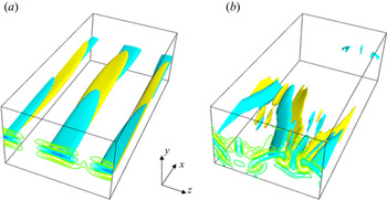
In both results, we see that the magnetic field decays in agreement with the asymptotic result, but the magnetic field generated in figure 1(d) is one order magnitude larger than that in figure 1(c). This difference is also reflected in the structure of the magnetic field, as shown in figure 4. Figures 4(a) and 4(b) show the streamwise current of the small amplitude solution (figure 1c) and the large amplitude solution (figure 1d), respectively. In figure 4(a) we can see that the structure of the solution is relatively simple, mainly because the perturbation energy is concentrated in the zeroth and first Fourier modes in the  $x$-direction. In contrast, the flow shown in figure 4(b) clearly has a more complicated structure in the
 $x$ direction.


The structure of the former type of solution is very similar to the purely hydrodynamic solutions typically found on the edge of laminar and turbulent attractors (Wang et al. Reference Wang, Gibson and Waleffe2007). As in the hydrodynamic case, the precise dynamo mechanism of the edge-state type solutions can be understood by a large-Reynolds-number asymptotic analysis, as we shall see in the next section. The asymptotic behaviour of solutions with large amplitudes is still unclear even for the hydrodynamic case and so no in-depth discussions will be presented in this paper (see Deguchi Reference Deguchi2019b also).
4. Results for large Reynolds numbers
4.1. Large-Reynolds-number limit of the Couette flow solutions
In this section we study the large-Reynolds-number asymptotic property of the solutions, fixing the magnetic Prandtl number and the periodic box to those used in the previous section. This means that we are considering the behaviour of vortices of about the channel width in a situation where both the hydrodynamic and magnetic Reynolds numbers are large. Note that, although the underlying philosophy of the asymptotic analysis is somewhat similar to the usual scaling arguments used in the turbulent physics community, the main question asked in the analysis is that if the assumed scaling is really mathematically consistent with the governing equations.
We consider asymptotic expansions of the physical quantities choosing the inverse of the Reynolds number as a small perturbation parameter. This is a singular perturbation problem and, in general, careful consideration is needed to find the appropriate expansions. In the current case, the expansions are similar to those obtained by Deguchi (Reference Deguchi2019a) for  $H = 0$. The main question here is how large the Hall parameter
 $H$ should be to balance the Hall term in the asymptotic structure. We shall see shortly that the appropriate size is
 $H=O(R^{-2/3})$; hence, hereafter we use the rescaled Hall parameter
 $H_0=R^{2/3}H$.
The asymptotic theory by Deguchi (Reference Deguchi2019a) is strongly motivated by the widely accepted sustainment mechanism of coherent structures in purely hydrodynamic shear flows; the streamwise mean flow (or roll–streak) produces unstable waves, which induce feedback to the mean field through the Reynolds stresses. This loop interaction between the mean flow and the wave is called the vortex-wave interaction (Hall & Smith Reference Hall and Smith1991) or self-sustaining process (Waleffe Reference Waleffe1997) in the shear flow community, and has many similarities with the mean-field dynamo theory. The unstable wave in MHD flows involves the Alfven wave which formally becomes singular in ideal approximation. As a result of the resonant absorption at the singular point, current sheets become prominent in the flow field, as frequently seen in many MHD simulations.
The form of the outer asymptotic expansions used by Deguchi (Reference Deguchi2019a) are
 \begin{gather} \left[ \begin{array}{c} u\\ v\\ w\\q \end{array} \right]= \left[ \begin{array}{c} \bar{u}(y,Z)\\ R^{{-}1}\bar{v}(y,Z)\\ R^{{-}1}\bar{w}(y,Z)\\ R^{{-}2}\bar{q}(y,Z) \end{array} \right] +R^{{-}7/6} \left \{ \exp({\textrm{i} \alpha (x-s_x t)}) \left[ \begin{array}{c} \tilde{u}(y,Z)\\ \tilde{v}(y,Z)\\ \tilde{w}(y,Z)\\ \tilde{q}(y,Z)\end{array} \right] +\text{c.c.} \right \}+\cdots, \end{gather}
 \begin{gather}\left[ \begin{array}{c} a\\b\\c \end{array} \right]= \left[ \begin{array}{c} R^{{-}1/3}\bar{a}(y,Z)\\ R^{{-}4/3}\bar{b}(y,Z)\\ R^{{-}4/3}\bar{c} (y,Z)\end{array} \right] +R^{{-}3/2} \left \{ \exp({\textrm{i} \alpha (x-s_xt)}) \left[ \begin{array}{c} \tilde{a}(y,Z)\\ \tilde{b}(y,Z)\\ \tilde{c}(y,Z)\\ \end{array} \right] +\text{c.c.} \right \}+\cdots, \end{gather}
where  $\alpha =2{\rm \pi} /L_x$ is the streamwise wavenumber,
 $Z=z-s_zt$,
 $s_z=R^{-1}s$ and c.c. stands for complex conjugate. The reason why those expansions are called ‘outer’ expansions is that different asymptotic expansions must be used within the resonant (or critical) layer.
In the expansions above we leave only the terms necessary to obtain the leading-order system. The first terms on the right-hand side are the leading-order part of the streamwise averaged field. Here and hereafter  $\bar {u}$ and
 $(\bar {v},\bar {w})$ are called streak and roll, respectively, and we adopt the same terminologies for the magnetic field components
 $\bar {a}$ and
 $(\bar {b},\bar {c})$. The second terms on the right-hand side are the leading-order part of the field fluctuating in the
 $x$ direction. There is only the fundamental Fourier mode in the
 $x$-direction; the asymptotic analysis can be used to verify that all the harmonics must be higher-order terms and do not participate in the leading-order system.
A feature of the roll–streak field is that it is  $x$-independent and, hence, is advected only by the rolls. The
 $R^{-1}$ scaling of the roll components was chosen to balance the viscous term and the advection term in the
 $x$-averaged equations. Similarly, the magnetic roll should be
 $R$ times smaller than the magnetic streak. However, the absolute magnitude of the magnetic roll–streak field cannot be determined from the outer problem, because outside the resonant layer the Lorentz force is negligible and, hence, the equations are linear with respect to the magnetic field. The analysis of the resonant layer is therefore necessary to complete the derivation of the asymptotic scaling, but before doing this we shall analyse the outer problem. Substituting the outer expansions into the governing equations (2.5) and only retaining the leading-order terms, it is easy to show that the roll–streak equations are viscous resistive as expected, i.e.
 \begin{gather} {}[\bar{v}\partial_y +(\bar{w}-s)\partial_Z-(\partial_y^2+\partial_Z^2)] \left[ \begin{array}{c} \bar{u}\\ \bar{v}\\ \bar{w} \end{array} \right] ={-}\left[ \begin{array}{c} 0\\ \partial_y\bar{q}\\ \partial_Z\bar{q} \end{array} \right],\end{gather}
 \begin{gather} {}[\bar{v}\partial_y +(\bar{w}-s)\partial_Z-P_m^{{-}1}(\partial_y^2+\partial_Z^2)] \left[ \begin{array}{c} \bar{a}\\ \bar{b}\\ \bar{c} \end{array} \right] -[\bar{b}\partial_y +\bar{c}\partial_Z] \left[ \begin{array}{c} \bar{u}\\ \bar{v}\\ \bar{w} \end{array} \right] \nonumber\\ =H_0 \left[ \begin{array}{c} 0\\\partial_Z(\bar{b}\partial_y\bar{a}+\bar{c}\partial_Z\bar{a}) \\ -\partial_y(\bar{b}\partial_y\bar{a}+\bar{c}\partial_Z\bar{a}) \end{array} \right], \end{gather}
 \begin{gather}\partial_y\bar{v}+\partial_Z\bar{w}=0, \quad \partial_y\bar{b}+\partial_Z\bar{c}=0. \end{gather}
On the other hand, all the dissipative effects are negligible in the wave part. After some manipulation, they can be combined into a single equation for the pressure wave
 \begin{equation} \partial_y \left ( \frac{\partial_y\tilde{q}}{(\bar{u}-s_x)^2} \right ) +\partial_Z \left ( \frac{\partial_Z\tilde{q}}{(\bar{u}-s_x)^2} \right ) -\alpha^2\frac{\tilde{q}}{(\bar{u}-s_x)^2} =0.\end{equation}
This equation becomes singular when  $\bar {u}-s_x$ vanishes; hereafter we denote this location as
 $y=f(Z)$. This singularity appears when the flow is viewed on the outer scale, but a close-up shows that it is actually regular due to the dissipative effects.
In order to analyse the behaviour of the outer solution around the singularity, it is convenient to introduce the coordinates  $(n,l)$ attached to the curve
 $y=f(Z)$ in the
 $y$–
 $Z$ plane; here we denote the signed length measured along straight lines that are normal to this curve as
 $n$, and the arc length measured along the curve as
 $l$. The usual regular singular point analysis for the outer wave equations tells us that as the singularity is approached the velocity wave amplitude is increased like
 $n^{-1}$, whilst the magnetic wave amplitude grows at an even faster rate proportional to
 $n^{-2}$. Those singular behaviours of the waves are, of course, resolved by the dissipative effects acting on a smaller scale. The thin dissipative layer surrounding the singularity is exactly what we called the resonant layer, where we must use the inner expansion. The layer thickness can be found by the viscous-convective balance for the wave equations. Let us assume that the dissipation effect in the wave equations is non-negligible in a layer of thickness
 $\delta$ around the curve
 $y=f(Z)$. By balancing the advection operator
 $(\bar {u}-s_x)\partial _x = O(\delta )$ and the viscous operator
 $R^{-1}\partial _y^2=O( R^{-1}\delta ^{-2})$, we arrive at
 $\delta =R^{-1/3}$ which is nothing but the well-known classical critical layer thickness.
The next thing we need to do is to see how the nonlinear self-interaction of the waves amplified around the resonant layer drive the roll components. First, we note that there are two kinds of nonlinear terms in the  $x$-averaged momentum equations, namely the Reynolds stress term and the Lorentz force term. The analysis of the former term is similar to the asymptotic structure derived in Hall & Sherwin (Reference Hall and Sherwin2010) for purely hydrodynamic shear flows. Let us denote the size of the velocity wave outside the resonant layer as
 $\rho$. Then the size of the wave inside the layer is found as
 $\rho \delta ^{-1}$ taking into account the effect of the singularity. Since the Reynolds stress only occurs inside the layer with thickness
 $\delta$, its size can be estimated to be
 $O((\rho \delta ^{-1})^2 \delta )$. From the requirement that this forcing should balance the viscous stress of the velocity roll of size
 $O(R^{-2})$, we have
 $\rho =\delta ^{1/2}R^{-1}=R^{-7/6}$ as seen in (4.1). Likewise, Deguchi (Reference Deguchi2019a) showed that within the resonant layer the Lorentz force affects the motion of the fluid, and, hence, the dynamo is not kinematic. The structure of this feedback effect is somewhat similar to that of the Reynolds stress term. However, as we have already seen, the magnetic wave component grows more rapidly around the singularity than the velocity counterpart. As a result, the amplitude of the magnetic wave outside the resonant layer must be
 $O(\delta \rho )=O(R^{-3/2})$, which is
 $O(\delta )$ times smaller than that for the velocity field (see (4.1)). The velocity roll field driven by those two nonlinear terms induces the streak due to the lift-up effect. The inhomogeneity that appeared in the streak field plays a crucial role in generating the waves as without it an inviscid instability is not possible.
The analysis of the  $x$-averaged induction equations is similar to what we saw in the momentum equations; the waves drive the magnetic roll (poloidal) component through the electromotive force in the resonant layer, and then the omega effect induces the magnetic streak (toroidal) component, as seen in Deguchi (Reference Deguchi2019a). Furthermore, we have to take account of the Hall effect as an additional wave forcing term. To balance the electromotive force by the wave with the Ohmic dissipation by the magnetic roll within the resonant layer, the magnetic roll–streak field must be
 $O(\delta )$ smaller than that of the velocity field, and, hence, the magnetic streak and roll in the outer scale must be
 $O(R^{-1/3})$ and
 $O(R^{-4/3})$, respectively. The magnitude of the Hall term is now completely determined by the analysis so far, because
 $H=O(R^{-2/3})$ must be chosen by the ratio of the hydrodynamic roll size
 $O(R^{-1})$ to the streak magnetic field size
 $O(R^{-1/3})$ in view of the outer roll–streak equation (4.2a). When this size of
 $H$ is adopted, the wave forcing due to the Hall effect in the roll system is in fact non-negligible within the resonant layer. Since the effect within the resonant layer is not trivial, a detailed matched asymptotic expansion analysis is needed here.
To this end, it is convenient to convert the  $y,z$ components of the fields into the
 $n,l$ components by introducing the unit vectors
 $\boldsymbol {e}_n$ and
 $\boldsymbol {e}_l$. The appropriate inner expansions for
 $u$,
 $a$,
 $\{(v,w)\cdot \boldsymbol {e}_n\}$,
 $\{(b,c)\cdot \boldsymbol {e}_n\}$,
 $\{(v,w)\cdot \boldsymbol {e}_l\}$,
 $\{(b,c)\cdot \boldsymbol {e}_l\}$ and
 $q$ are as follows: for the wave components,
 \begin{gather} \delta^{{-}1}R^{{-}7/6}\tilde{U}_0(N,l)+\cdots,\quad \delta^{{-}2}R^{{-}3/2}\tilde{A}_0(N,l)+\cdots, \end{gather}
 \begin{gather}R^{{-}7/6}\tilde{V}_0(N,l)+\cdots,\quad \delta^{{-}1}R^{{-}3/2}\tilde{B}_0(N,l)+\cdots, \end{gather}
 \begin{gather}\delta^{{-}1}R^{{-}7/6}\tilde{W}_0(N,l)+\cdots,\quad \delta^{{-}2}R^{{-}3/2}\tilde{C}_0(N,l)+\cdots, \end{gather}
and  $R^{-7/6}\tilde {Q}_0(l)+\cdots$, respectively, and for the roll–streak components,
 \begin{gather} s_x+\delta \lambda(l)N+\cdots,\quad R^{{-}1/3}\gamma(l)+\cdots,\hspace{20mm} \end{gather}
 \begin{gather}R^{{-}1}\{\bar{V}_0(l)+\delta \bar{V}_1(N,l)\}+\cdots,\quad R^{{-}4/3}\{\bar{B}_0(l)+\delta \bar{B}_1(N,l)\}+\cdots, \end{gather}
 \begin{gather}R^{{-}1}\{\bar{W}_0(l)+\delta \bar{W}_1(N,l)\}+\cdots,\quad R^{{-}4/3}\{\bar{C}_0(l)+\delta \bar{C}_1(N,l)\}+\cdots \end{gather}
and  $R^{-2}\bar {Q}_0(N,l)+\cdots$, respectively. Here
 $N=n/\delta$ is the stretched normal coordinate appropriate to the inner scale. The leading-order wave equations are found as
 \begin{gather} \textrm{i}\alpha (\lambda N \tilde{U}_0 -\gamma \tilde{A}_0)+\lambda \tilde{V}_0+\lambda'N\tilde{W}_0-\gamma '\tilde{C}_0={-}\textrm{i}\alpha \tilde{Q}_0 +\partial_N^2\tilde{U}_{0}, \end{gather}
 \begin{gather}\textrm{i}\alpha (\lambda N \tilde{W}_0 -\gamma \tilde{C}_0)={-}\partial_l\tilde{Q}_{0}+\partial_N^2\tilde{W}_{0}, \end{gather}
 \begin{gather}\textrm{i}\alpha (\lambda N \tilde{A}_0 -\gamma \tilde{U}_0)-\lambda \tilde{B}_0-\lambda'N \tilde{C}_0+\gamma '\tilde{W}_0=P_m^{{-}1}\partial_N^2\tilde{A}_{0}, \end{gather}
 \begin{gather}\textrm{i}\alpha (\lambda N \tilde{B}_0 -\gamma \tilde{V}_0)=P_m^{{-}1}\partial_N^2\tilde{B}_{0}, \end{gather}
 \begin{gather}\textrm{i}\alpha (\lambda N \tilde{C}_0 -\gamma \tilde{W}_0)=P_m^{{-}1}\partial_N^2\tilde{C}_{0}, \end{gather}
 \begin{gather}\textrm{i}\alpha \tilde{U}_0+\partial_N\tilde{V}_{0}+\partial_l\tilde{W}_{0}=0, \end{gather}
 \begin{gather}\textrm{i}\alpha \tilde{A}_0+\partial_N\tilde{B}_{0}+\partial_l\tilde{C}_{0}=0. \end{gather}
Of the leading-order roll–streak equations, the important ones are the  $N$ and
 $l$ components of the momentum equations, and the
 $l$ component of the induction equations. Integrating them in the
 $N$-direction, we have the conditions
 \begin{gather} {}[\bar{Q}_0]^{\infty}_{-\infty}=\chi \int^{\infty}_{-\infty}(|\tilde{W}_0|^2-|\tilde{C}_0|^2)\,\textrm{d}N+\text{c.c.}, \end{gather}
 \begin{gather}{}[\bar{W}_{1N}]^{\infty}_{-\infty}=\frac{\partial}{\partial l}\int^{\infty}_{-\infty}(|\tilde{W}_0|^2-|\tilde{C}_0|^2)\,\textrm{d}N+\text{c.c.}, \end{gather}
 \begin{gather}{}[\bar{C}_{1N}]^{\infty}_{-\infty}=P_m\chi \int^{\infty}_{-\infty} (\tilde{B}_0\tilde{W}_0^*-\tilde{V}_0\tilde{C}_0^*)+P_mH_0\left (\tilde{B}_0\frac{\partial \tilde{A}_{0}^*}{\partial N}+\tilde{C}_0^*\frac{\partial \tilde{A}_{0}}{\partial l}\right )\,\textrm{d}N +\text{c.c.}, \end{gather}
where the asterisk represents complex conjugation, and  $\chi (l)=-f''/(1+f'^2)^{3/2}$ is the curvature of the resonant layer.
In principle, we can find the solutions of the wave equations (4.6) by matching them to the outer solution, and use them to work out the right-hand sides of (4.7). Therefore, the upshot of the inner analysis is that we can express the jumps  $[\bar {q}]^{0_+}_{n=0_-}$,
 $[\{(\bar {v},\bar {w})\cdot \boldsymbol {e}_l\}_n]^{0_+}_{n=0_-}$ and
 $[\{(\bar {b},\bar {c})\cdot \boldsymbol {e}_l\}_n]^{0_+}_{n=0_-}$ in terms of
 $\chi$ and the values of
 $\bar {u}_n$,
 $\bar {a}$,
 $\tilde {q}$ at
 $y=f(Z)$; in particular, when
 $P_m=1$, we can derive an analytic expression of the jumps as shown in Appendix A. The important point here is that the outer roll–streak equations (4.2), the outer pressure wave equation (4.3) and the jumps form a closure for the leading-order flow. Physically, the jumps are energy injections from the waves to the rolls, of which the Hall effect cannot be neglected in those resulting from the induction equation. The jump in the induction equations essentially corresponds to those empirically modelled by the alpha effect in the mean-field dynamo theory.
The scaling described above can be confirmed in the numerical solution. It has already been shown by Deguchi (Reference Deguchi2019b) for pure MHD flows that the edge-state type solutions behave in a manner consistent with the asymptotic theory. The solution at point A in figure 1(a) was used in this study. Using the same solution, here we shall check if the scaling of the Hall effect derived above can be observed. In order to obtain a sufficiently accurate asymptotic scaling in the numerical computation, the Reynolds number of the solution is increased up to  $30\,000$. The computation requires higher resolution in the
 $y$ and
 $z$ directions because, as the theoretical result tells, the resonant layer gets thinner. Figure 5 shows the result of changing
 $H$ from point A for
 $R=20\,000$ and 30 000. The quantity
 $I_z$ defined in (2.11a,b) is one of the appropriate quantities to measure the magnitude of the magnetic roll. This component is associated with the roll field and, thus, should be scaled by
 $R^{4/3}$ because of the expansion (4.1). Indeed, in figure 5(a) the results for the two different
 $R$ collapse onto a single curve after rescaling
 $H$ by
 $R^{2/3}$, and
 $I_z$ by
 $R^{4/3}$. To check this collapse is not a coincidence, a similar comparison is made for
 $I_x$, as shown in figure 5(b). In this figure
 $I_x$ is rescaled by
 $R^{1/3}$ because it measures the magnitude of the magnetic streak; see (4.1). We also checked that no inconsistency with the theory was found using other physical quantities such as the energy of each component.
The large  $R$ convergence of the solution branch. The green dashed and blue dotted curves are computed at
 $R=20\,000$ and
 $R=30\,000$, respectively. In order to compute the high-Reynolds-number solutions we have increased the number of the Chebychev polynomials and the Fourier harmonics in the
 $z$ direction to 100 and 28, respectively. While thanks to the asymptotic property of the edge-state type solutions, we only need three or four Fourier harmonics in the
 $x$ direction.

4.2. Vertically localised states
In this section we will discuss what would happen if the sides of the periodic box  $L_x$ and
 $L_z$, which were fixed in the previous section, are reduced in dependence on the Reynolds number. For the sake of simplicity, we fix the ratio
 $L_x/L_z$ and consider a situation where both
 $L_x$ and
 $L_z$ are scaled by
 $h\ll 1$. This is an interesting question as it is well known that fine eddies typically appear at high-Reynolds-number turbulent flows. For the purely hydrodynamic cases, a similar computation has been independently performed by Blackburn et al. (Reference Blackburn, Hall and Sherwin2013) and Deguchi (Reference Deguchi2015), where the results showed that all nonlinear effects are concentrated within a layer of depth
 $h$, which we hereafter call the production layer.
For the MHD problem, similar localisation can be observed as shown in figure 6. The asymptotic property of the localised solution can be easily found. Outside the production layer there is merely a linear shear which is almost the laminar Couette flow. We require that the shear  $\partial _y u$ is
 $O(1)$ there, so
 $u$ must be scaled as
 $O(h)$ in the production layer. After rescaling
 $\boldsymbol {v}$,
 $\boldsymbol {b}$,
 $p$ and
 $H$ by
 $h,h,h^2$ and
 $h$, respectively, it is easy to see that the new Reynolds number becomes
 $Rh^2$. As long as this ‘effective Reynolds number’ is large, the matched asymptotic expansion analysis, as in the previous section, is possible for the nonlinear structures in the production layer. The structure of this asymptotic regime analogues to that found in Blackburn et al. (Reference Blackburn, Hall and Sherwin2013). When
 $h$ is
 $O(R^{-1/2})$, i.e. at the Kolmogorov microscale, the effective Reynolds number becomes
 $O(1)$, and, hence, all the terms in the governing equations must be retained, similar to the hydrodynamic version by Deguchi (Reference Deguchi2015). The maximum Hall parameter we can take is
 $H=O(R^{-1/2})$, which is much larger than
 $H=O(R^{-2/3})$ found in the previous section.
The solutions computed for small  $L_x$ and
 $L_z$. Point
 $D$ shown in figure 7(b) is used. All the fluctuations are localised in the production layer, as shown by the isosurfaces of the streamwise current (see figure 2 for the definition) and the streamwise magnetic field (the colour map on the back). In the upper and lower outer regions, the flow is merely a linear shear to leading order. Results are shown for (a)
 $R=10\,000$, (b)
 $R=30\,000$.

The above order-to-magnitude estimate can be refined a bit more, using the fact that the flow outside of the production layer is not completely the laminar Couette flow. Let us consider the Kolmogorov microscale states localised in the production layer, and assume that it is sandwiched by the upper and lower outer regions (see figure 3 of Deguchi Reference Deguchi2017). We denote the streamwise and spanwise drag on the wall as  $D_x$ and
 $D_z$, respectively. Then to leading order the velocity
 $\boldsymbol {v}$ in the upper and lower outer regions must be written in the form
 \begin{equation} (D_xy- D_x+ 1,0,D_z y - D_z)\quad \text{and}\quad (D_xy+ D_x- 1,0,D_z y + D_z), \end{equation}
respectively. Note that the mean shear should not change across the production layer, and the outer flows should satisfy the boundary conditions. Likewise using  $I_x$ and
 $I_z$ defined in (2.11a,b), the leading-order magnetic fields
 $\boldsymbol {b}$ in the upper and lower outer regions are written as
 \begin{equation} (I_x y - I_x, 0, I_z y - I_z)\quad \text{and}\quad (I_x y + I_x, 0, I_z y + I_z), \end{equation}
respectively.
The equations satisfied by the canonical structure within the production layer should be found using the rescaled variable  $(X,Y,Z)=h^{-1}(x,y,z)$, assuming that the centre of the layer is at
 $y=0$ (it is easy to extend the theory to general cases). Requiring that the rescaled equations must have a unit effective Reynolds number, the appropriate scaling can be found as
 \begin{equation} \boldsymbol{v}=\frac{1}{Rh}\boldsymbol{V}(X,Y,Z,T),\quad \boldsymbol{b}=\frac{1}{Rh}\boldsymbol{B}(X,Y,Z,T),\quad p=\frac{1}{R^2h^2}P(X,Y,Z,T), \end{equation}
where  $T=t/(Rh^2)$. In fact, by writing
 $H=h\hat {H}$, the governing equations become
 \begin{gather} (\partial_T+\boldsymbol{V}\boldsymbol{\cdot} \widehat{\boldsymbol{\nabla}})\boldsymbol{V} - (\boldsymbol{B}\boldsymbol{\cdot} \widehat{\boldsymbol{\nabla}})\boldsymbol{B} ={-}\boldsymbol{\nabla} P + \widehat{\nabla}^2 \boldsymbol{V}, \end{gather}
 \begin{gather}\partial_T\boldsymbol{b} = \widehat{\boldsymbol{\nabla}} \times [(\boldsymbol{V}-\hat{H}\widehat{\boldsymbol{\nabla}} \times \boldsymbol{B})\times \boldsymbol{B}]+\frac{1}{P_m} \widehat{\nabla}^2 \boldsymbol{B}, \end{gather}
 \begin{gather}\widehat{\boldsymbol{\nabla}} \boldsymbol{\cdot} \boldsymbol{V} =0,\quad \widehat{\boldsymbol{\nabla}} \boldsymbol{\cdot} \boldsymbol{B}=0, \end{gather}
where  $\widehat {\boldsymbol {\nabla }}=(\partial _X,\partial _Y,\partial _Z)$. Here the periodicities of the flow in
 $X,Z$ become
 \begin{equation} [\boldsymbol{V},\boldsymbol{B}](X,Y,Z,T)=[\boldsymbol{V},\boldsymbol{B}](X+L_{x0},Y,Z,T)=[\boldsymbol{V},\boldsymbol{B}](X,Y,Z+L_{z0},T), \end{equation}
with the normalised periodicity  $L_{x0}=L_x/h$,
 $L_{z0}=L_z/h$. For the normal direction, we require that on exiting the layer the rescaled velocity tends to
 $Y$ to leading order so that
 \begin{equation} \boldsymbol{V}\rightarrow (Y\mp D_{x0},0,\mp D_{z0}),\quad \boldsymbol{B}\rightarrow ({\mp} I_{x0}, 0,\mp I_{z0}) \end{equation}
as  $Y\rightarrow \pm \infty$. Here
 $D_{x0}, D_{z0}, I_{x0}$ and
 $I_{z0}$ are constants determined by solving the canonical problem (4.11), and, hence, they are functions of
 $L_{x0}, L_{z0}, P_m$ and
 $\hat {H}$.
The scaling factor  $h$ must be fixed by matching the production layer solutions with the outer solutions. Let us compare the outer solution (4.8a,b) rewritten in terms of the production layer variable
 $Y$ and the limiting behaviour of the inner solution (4.11e),
 \begin{equation} Rh(1-D_x+D_xhY)\approx Y-D_{x0}. \end{equation}
From the coefficients of  $Y^0$ and
 $Y^1$, we have
 \begin{equation} D_x\approx 1+\frac{D_{x0}}{Rh},\quad D_x\approx \frac{1}{Rh^2}, \end{equation}
respectively. Thus, to leading order the drag  $D_x$ is unity, and
 $h=R^{-1/2}$ as we obtained earlier. The formal asymptotic analysis yields that within the production layer the leading-order flow satisfies (4.11), and creates the small jump in the streamwise velocity across the layer. This jump is the origin of the small next-order correction
 ${D_{x0}}/{R^{1/2}}$ to the drag.
However, in order to observe the asymptotic convergence of the finite-Reynolds-number result, it is more convenient to use the scaling factor
 \begin{equation} h=\frac{1}{\sqrt{D_{x}R}}\end{equation}
directly deduced from the second equation in (4.13a,b). The difference to the previous one is that some higher-order terms seen in the approximation of  $D_x$ are incorporated into the scaling. This is beneficial in observing a better asymptotic convergence in the numerical result, because some of the next-order correction terms in the asymptotic analysis can be retained. Figure 7(a) is the numerical results obtained by reducing
 $L_x$ and
 $L_z$ from the solution seen in figure 5, and figure 7(b) is their rescaled version. Here, we consider the asymptotic convergence of
 $I_x$. The scaling is motivated by the fact that
 $I_{0x}$ appeared in (4.11e) is a function of
 $L_{z0}=L_z/h$. Comparing the outer solution (4.9a,b) and the limiting inner solution (4.11e), we have
 \begin{equation} Rh({-}I_x+I_xhY) \approx{-}I_{0x}, \end{equation}
from which to leading order we have  $Rh I_x=I_{0x}$. In figure 7(b) the horizontal and vertical axes are
 $1/L_{0x}$ and
 $I_{0x}$, and, hence, as expected, we can observe the convergence towards the canonical result with increasing the Reynolds number. In this figure,
 $h$ is the one defined in (4.14). If we use the simpler
 $h=R^{-1/2}$, the convergence will be worse and we will need to use a larger Reynolds number.
(a) The behaviour of the solutions for small  $L_x$ and
 $L_z$. The ratio
 $L_x/L_z$ is fixed to 2 in this figure. The solution branch is continued from that shown in figure 5. The red solid, green dashed and blue dotted curves are the result for
 $R=10\,000$, 20 000 and 30 000, respectively. Panel (b) is the same result but with the rescaling obtained by the theory. Typically 180 Chebyshev polynomials are used in
 $y$, while in the
 $x$ and
 $z$ directions up to 6th and 24th harmonics are retained, respectively.

4.3. The high-Reynolds-number solution in a shearing box
The fact that the nonlinear interaction is maintained even away from the wall suggests that the theoretical result so far can be extended to more general situations. For example, the localised canonical structure can be embedded for any  $y$ by using the Galilean transform to make the streamwise phase velocity almost the same as the laminar velocity. Moreover, we can even embed multiple nonlinear solutions in the flow, as long as they are far enough apart from each other.
In the case the coherent structures are placed closely, we need to include some interaction between them. For effective Reynolds number of order unity, the simplest way to incorporate such an interaction is to use a framework called the shearing box, which is a common way to study distributed coherent structures (Schumann Reference Schumann1985; Gerz, Schumann & Elgobashi Reference Gerz, Schumann and Elgobashi1989; Brandenburg et al. Reference Brandenburg, Nordlund, Stein and Torkelsson1995; Hawley, Gammie & Balbus Reference Hawley, Gammie and Balbus1995). The flow configuration considered in this framework is similar to plane Couette flow but the walls are replaced by the shear-periodic condition – namely the flow is required to be invariant by moving the flow in the  $y$ direction for one period and then Galilean transforming it in the
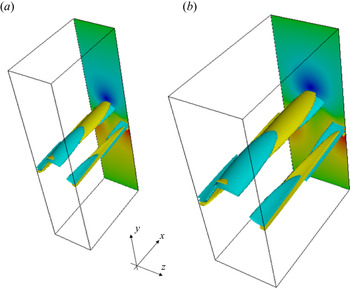
 $x$ direction for the same period. Finding nonlinear solutions in the shearing box at high Reynolds numbers is not an easy task (Sekimoto & Jiménez Reference Sekimoto and Jiménez2017). However, when the effective Reynolds number is sufficiently large, Blackburn et al. (Reference Blackburn, Deguchi and Hall2021) recently showed that the asymptotic theory by Hall (Reference Hall2018) can be used to compute the solutions more easily. Here we shall briefly see that such a computation is also possible for MHD flows.
Figure 8 shows the MHD dynamo solution found by this method. The computation can be done by applying a minor modification to the existing numerical code as follows. First, as we are assuming a high effective Reynolds number of the flow, we can apply the asymptotic theory seen in § 4.1. We treat the roll–streak and wave components of the flow separately. For the shearing box problem, the roll–streak component ( $x$-independent part) should be described by the sum of the laminar homogeneous shear and the perturbation field which is periodic in the
 $y$ direction. Therefore, in the numerical computation, we simply need to replace the Chebyshev polynomials with Fourier modes for this component. In figure 8 we plotted 1.5 periods of the solution in
 $y$. As can be seen in the figure, there are two symmetrically arranged waves in one period. Looking at the central half-period box, we can see that the basic structure of the solution is very similar to that found in the Couette flow (see figure 2a). Recall that the wave is induced by the instability of the streak field. The streak field is not periodic due to the inclusion of the laminar homogeneous shear flow, and, thus, the generated wave component is not periodic in
 $y$. However, the shear-periodic condition is nevertheless satisfied by the periodic arrangement of the waves with different speeds appropriate to each half-periodic cell (see Blackburn et al. Reference Blackburn, Deguchi and Hall2021 for detail). Here we computed only the central wave and used its copies to calculate the periodic feedback to the roll component. The amplitude of the central wave decreases rapidly as moving away from the half-periodic box at the centre. Practically, it is sufficient to use the computational domain about three times larger than the roll–streak period, so again the modification to the numerical code is not too difficult.
The dynamo solution in the shearing box at  $R=10\,000$. See figures 2 and 6 for the definition of the surfaces and the colour map. Translucent surfaces are used except for the central wave. The dimension of the box shown is
 $[0, 2{\rm \pi} ]\times [-3,3]\times [0,{\rm \pi} ]$. The wave is resolved by using 260 Chebyshev polynomials in
 $y$, and taking up to 20th Fourier harmonics in
 $z$. For the roll–streak component up to 60th Fourier harmonics are used in
 $y$. Note that in this figure, the size of the central half-period box is the same as that used in figures 2 and 4.

4.4. Induction through the free-stream coherent structure mechanism
When a localised solution such as the one discussed in § 4.2 occurs in a boundary layer flow, an interesting phenomenon occurs. The results in this section are an extension of the purely hydrodynamic study by Deguchi & Hall (Reference Deguchi and Hall2014b), where it is shown that a small three-dimensional equilibrium solution placed in the vicinity of the free stream has the ability to produce even larger disturbances in the boundary layer (see figure 2 of Deguchi & Hall Reference Deguchi and Hall2017). This amplification mechanism is due to the lift-up effect where the roll drives the streak. Here we shall see in the MHD version that the growth also occurs in the magnetic field through the omega effect.
For the sake of simplicity, here we consider the asymptotic suction boundary layer flow with the base flow profile  $\boldsymbol {v}=(1-\textrm {e}^{-y},-R^{-1},0)$, where
 $y$ is the distance from the wall. For large
 $y$, the flow approaches a uniform free stream. We impose periodicity in the
 $x$ and
 $z$ directions with the fixed periods
 $L_x$ and
 $L_z$, respectively. The key point of the theory is that the unit effective Reynolds number nonlinear states are operational without changing the length scale, if the velocity is scaled like
 $O(R^{-1})$ in the Navier–Stokes equations. Of course the question is whether the base flow will allow this scaling. Deguchi & Hall (Reference Deguchi and Hall2014b) showed for the asymptotic suction boundary layer flow that such a situation indeed occurs when the base shear
 $\textrm {e}^{-y}$ becomes
 $O(R^{-1})$, i.e. when
 $y$ is
 $O(\ln R)$ (note that a Galilean transformation can be used to eliminate the constant part so we only need to check the size of the base shear). This is the location of the production layer, which in this case coincides with what is known as the edge layer in the boundary layer transition studies (Duck, Ruban & Zhikharev Reference Duck, Ruban and Zhikharev1996). Some readers may think that the theory is probably only applicable to the simple model flow, but note that for any boundary layer flows, the effective Reynolds number decreases as it approaches the free stream. The truth is that, somewhat surprisingly, the same production layer solution in the asymptotic suction boundary layer is generic to many non-parallel boundary layer flows (Deguchi & Hall Reference Deguchi and Hall2015) and jet flows (Deguchi & Hall Reference Deguchi and Hall2018).
Let us consider a pure MHD flow ( $H = 0$) in the asymptotic suction boundary layer flow. We assume that the wall is insulating as in the previous sections. The production layer problem (4.11) with
 $\hat {H}=0$ can be found by applying the coordinate transform
 $(X,Y,Z,T)=(x-t,y-\ln R,z,R^{-1}t)$, and writing
 \begin{gather} \boldsymbol{v}=(1,0,0)+R^{{-}1}\boldsymbol{V}(X,Y,Z,T)+\cdots, \end{gather}
 \begin{gather}p=R^{{-}2}P(X,Y,Z,T)+\cdots,\quad \boldsymbol{b}=R^{{-}1}\boldsymbol{B}(X,Y,Z,T)+ \cdots \end{gather}
in the governing equations (2.5). The boundary conditions for the production layer problem are the periodic conditions
 \begin{equation} [\boldsymbol{V},\boldsymbol{B}](X,Y,Z,T)=[\boldsymbol{V},\boldsymbol{B}](X+L_{x},Y,Z,T)=[\boldsymbol{V},\boldsymbol{B}](X,Y,Z+L_{z},T), \end{equation}
and the far-field conditions
 \begin{gather} (U,V,W,A,B,C)\rightarrow (0,-1,0,0,0,0)\quad \text{as} \ Y\rightarrow \infty, \end{gather}
 \begin{gather}(Ue^Y,V,W,Ae^Y,B,C)\rightarrow ({-}1,-1,0,0,0,0)\quad \text{as} \ Y\rightarrow -\infty. \end{gather}
The latter conditions require that, for large negative  $Y$, the flow goes back to the laminar flow to leading order. However, note that (4.18b) allows some exponential growth of perturbation at slower rate than that of the base flow.
As the nonlinearity is assumed to be localised within the production layer, the growth of the perturbation as  $Y\rightarrow -\infty$ can be seen by analysing the linearised equations. As shown in Deguchi & Hall (Reference Deguchi and Hall2014b), the
 $x$ dependent part must be more rapidly damped than the roll–streak component in this limit. Furthermore, among the roll components the harmonics decay more rapidly than the fundamental mode as they feel the viscous effect more strongly. Let us write the wavenumber of the fundamental mode as
 $\beta$ (note that it does not necessarily equal to
 ${2{\rm \pi} }/{L_z}$, see Deguchi & Hall Reference Deguchi and Hall2014b, Reference Deguchi and Hall2017). Then the limiting behaviour of
 $(V,W)$ and
 $(B,C)$ as
 $Y\rightarrow -\infty$ may be written as
 \begin{equation} (\mathcal{V}(Y)\cos \beta z,\mathcal{W}(Y)\sin \beta z)+\cdots \quad \text{and}\quad (\mathcal{B}(Y)\cos \beta z,\mathcal{C}(Y)\sin \beta z)+\cdots, \end{equation}
respectively. Here the functions  $\mathcal {V}(Y)$ and
 $\mathcal {B}(Y)$ must satisfy
 \begin{gather} (\partial_Y+\partial_Y^2-\beta^2)(\partial_Y^2-\beta^2)\mathcal{V}=0, \end{gather}
 \begin{gather}(\partial_Y+P_m^{{-}1}(\partial_Y^2-\beta^2))\mathcal{B}=0, \end{gather}
from the linearised roll equations, and  $\mathcal {W}(Y)=-\beta ^{-1}\mathcal {V}'$,
 $\mathcal {C}(Y)=-\beta ^{-1}\mathcal {B}'$ from the continuity and Gauss's law. Solving (4.20) and looking for the slowest decaying mode we find that the leading-order behaviour of the roll components
 \begin{equation} \mathcal{V}(Y)\sim K\textrm{e}^{\omega Y}, \quad \mathcal{B}(Y)\sim J\textrm{e}^{\gamma Y} \end{equation}
as  $Y\rightarrow -\infty$. Here
 \begin{equation} \omega=\frac{1}{2}\left(\sqrt{1+4\beta^2}-1\right)>0,\quad \gamma=\frac{1}{2}\left(\sqrt{P_m^2+4\beta^2}-P_m\right)>0 \end{equation}
and  $J$ and
 $K$ are constants determined by the production layer solution. The reason for discarding the exponentially increasing mode in (4.20a) is that if they were present, nonlinearities would appear, violating the assumption. The roll component is hence attenuated, but it interacts with the base flow through the lift-up term to promote the streak growth. Importantly, this growth does not produce any nonlinear effect. Let us write the leading-order behaviour of
 $U$ and
 $A$ as
 \begin{equation} \mathcal{U}(Y)\cos \beta z+\cdots \quad \text{and}\quad \mathcal{A}(Y)\cos \beta z+\cdots, \end{equation}
respectively. The behaviour of the functions  $\mathcal {U}(Y)$ and
 $\mathcal {A}(Y)$ can be found from the linearised streak equations
 \begin{align} (\partial_Y+\partial_Y^2-\beta^2)\mathcal{U}=\textrm{e}^{{-}Y}\mathcal{V}, \end{align}
 \begin{align} (\partial_Y+P_m^{{-}1}(\partial_Y^2-\beta^2))\mathcal{A}={-}\textrm{e}^{{-}Y}\mathcal{B}, \end{align}
from which we can find
 \begin{equation} \mathcal{U}(Y)\sim{-}\frac{K\textrm{e}^{(\omega-1) Y}}{2\omega},\quad \mathcal{A}(Y)\sim \frac{P_m J \textrm{e}^{(\gamma-1) Y}}{P_m+2\gamma -1}, \end{equation}
as  $Y\rightarrow -\infty$. Therefore, the growth of the hydrodynamic streak occurs when
 $\omega -1<0$, i.e.
 $\beta <\sqrt {2}$ as seen in Deguchi & Hall (Reference Deguchi and Hall2014b), while the condition for the magnetic field growth can be found as
 \begin{equation} \beta<\sqrt{1+P_m}, \end{equation}
which ensures  $\gamma -1<0$. Moreover,
 $({\partial }/{\partial P_m})(\gamma -\omega )<0$ implies that
 \begin{align} \gamma > \omega \quad \text{if} \ P_m<1, \end{align}
 \begin{align} \gamma \leq \omega \quad \text{if} \ P_m\geq 1. \end{align}
Therefore, when  $P_m>1$ (
 $P_m< 1$), the magnetic streak grows faster (slower) than the hydrodynamic part.
The leading-order field in the boundary layer can be found by seeking a linearised roll–streak solution that matches the above far-field behaviour of the production layer solution when  $y$ is large and satisfies the boundary conditions at
 $y=0$. The hydrodynamic part of the leading-order boundary layer solution can be seen in Deguchi & Hall (Reference Deguchi and Hall2014b). Similarly, after some algebra, the leading-order magnetic field can be found as
 \begin{equation} a=R^{-\gamma}F(y)\cos \beta z+\cdots,\end{equation}
where
 \begin{equation} F(y)=P_mJ\left \{ \frac{(\textrm{e}^{(\gamma-1)y}-\textrm{e}^{-(\gamma+P_m)y})}{P_m+2\gamma-1} +\frac{(\beta-\gamma)(\textrm{e}^{-(P_m+\gamma+1)y}-\textrm{e}^{-(\gamma+P_m)y})}{(P_m+1)(P_m+\gamma+\beta)(2P_m+2\gamma+1)}\right \}.~~~~~~ \end{equation}
The function  $F(y)$ is shown in figure 9(a) for
 $\beta =1$ and various
 $P_m$. For this value of
 $\beta$, consistent with (4.27), no matter how small
 $P_m$ is the growth of the magnetic streak occurs towards the wall. Moreover, the larger the value of
 $P_m$ is, the more rapidly the magnetic field increases. Note that the behaviour of the hydrodynamic streak is similar to the
 $P_m=1$ result shown in this picture, as highlighted by the thick green dashed curve. When the value of
 $\beta$ is increased to
 $2$, as shown in figure 9(b), the growth of the hydrodynamic streak is suppressed because the growth condition
 $\beta <\sqrt {2}$ is violated. Nevertheless, when
 $P_m>3$, the growth of the magnetic streak occurs; see (4.27).
The near-wall perturbation driven by a small nonlinear perturbation in the production layer at  $y=\ln R$. The amplitude
 $F(y)$ of the magnetic field in the boundary layer for
 $P_m=0.2$, 0.6, 1.0, 1.4, 1.8, 2.2, 2.6, 3.0, 3.4, 3.8 and 4.2. The result for
 $P_m=1$ is highlighted by the green dashed curve. Results are shown for (a)
 $\beta =1$, (b)
 $\beta =2$.

Now we include the Hall effect in the flow, considering  $H>0$. A simple order-to-magnitude analysis shows that as long as
 $H$ is smaller than
 $O(1)$, the leading-order structure of the production layer remains unchanged. However, even if
 $H$ is small, the structure of the amplified magnetic field below the layer will be affected. To see this, we treat
 $H$ as a perturbation to the asymptotic structure obtained for the pure MHD. For example, the magnetic field can be expanded as
 \begin{equation} \boldsymbol{b}=R^{{-}1}\{\boldsymbol{B}(X,Y,z)+H\boldsymbol{B}_1(X,Y,z)+\cdots\}. \end{equation}
In order to analyse the region beneath the production layer, it is convenient to introduce the new stretched variable  $\xi =y/(\ln R)$, where
 $\xi =1$ and 0 correspond to the locations of the production layer and the boundary layer, respectively. The solution we developed earlier is valid for
 $\xi \in (\xi _c,1)$, where
 $\xi _c$ is the position at which the leading-order structure breaks down due to the Hall effect. The scenario of the breakdown is as follows. (i) First we note that a growing
 $y$-
 $z$ mean magnetic field can be generated by the electromotive force. The size of the forcing can be found by the interaction of the magnetic streak and the hydrodynamic roll. (ii) The magnetic roll component in
 $\boldsymbol {B}_1$ is driven by the Hall term, whose leading-order part comes from the interaction of the mean magnetic field and the magnetic roll in
 $\boldsymbol {B}$. This forcing can grow beneath the production layer, and, thus, the next-order magnetic roll can also grow towards the wall. (iii) In summary, the magnetic roll component in
 $\boldsymbol {B}$ should decay, but that in
 $\boldsymbol {B}_1$ can grow. The breakdown of the asymptotic expansion occurs when
 $\boldsymbol {B}$ and
 $H\boldsymbol {B}_1$ become the same size. At this breakdown point, we need to solve a nonlinear induction equation, similar to what we saw in § 3.1. The nonlinearity suppresses the growth of the magnetic field for
 $\xi <\xi _c$.
To determine  $x_c$, the size of each component appeared in the above argument needs to be identified as follows.
(i) We already know the behaviour of the leading-order roll–streak as seen in (4.21a,b) and (4.26a,b). Using
$Y=(\ln R)(\xi -1)$ and recalling (4.16), the size of them in terms of the original variables $\boldsymbol {v},\boldsymbol {b}$ can be found as shown in table 2. For example, the size of the magnetic streak is $O(R^{-1}\textrm {e}^{(\gamma -1)Y})=O(R^{(\xi -1)(\gamma -1)-1})$. At the boundary layer ($\xi =0$), the size is $O(R^{-\gamma })$ which is consistent with our earlier result (4.30).(ii) Next, we estimate the size of the
$x$–$z$ averaged part of the perturbation. The mean magnetic field is driven by the electromotive force. The behaviour of this forcing term can be found as $\textrm {e}^{(\omega +\gamma -1)Y}$ by multiplying the magnetic streak and the hydrodynamic roll. The mean field behaves like this forcing as $Y\rightarrow -\infty$. The behaviour of the hydrodynamic part can be found in a similar manner by noting that it is driven by the Reynolds stress and the Lorentz force.(iii) Finally, we consider the roll component in
$\boldsymbol {B}_1$. This component satisfies an equation similar to (4.25), but forced by the Hall term. As the leading-order part of the forcing comes from the interaction of the magnetic mean field and the magnetic roll component, it behaves like $\textrm {e}^{(2\gamma +\omega -1)Y}$. The size of the next-order roll in terms of the original variable is $O(R^{-1}He^{(2\gamma +\omega -1)Y})=O(HR^{(\xi -1)(2\gamma +\omega -1)-1})$.


The size of the perturbation beneath the production layer. Here  $\xi =1$ is the location of the production layer, and
 $\xi =0$ corresponds to the boundary layer. Note that the hydrodynamic components do not include the base flow. The roll, streak and mean components refer to the poloidal, toroidal, and
 $x$–
 $z$ averaged fields, respectively.

The asymptotic expansion breaks down when  $O(R^{(\xi -1)\gamma -1})=O(HR^{(\xi -1)(2\gamma +\omega -1)-1})$. The critical value
 $\xi _c$ can be found by solving
 $R^{(\xi _c-1)\gamma -1}=HR^{(\xi _c-1)(2\gamma +\omega -1)-1}$, i.e.
 \begin{equation} \xi_c=\frac{\ln (HR^{1-\gamma-\omega})}{\ln (R^{1-\gamma-\omega})}. \end{equation}
The above discussion holds even when the effective Reynolds number in the production layer is large, but the scaling becomes a bit more complicated.
5. Conclusion
The nonlinear coherent structures and their associated dynamo mechanism have been studied for Hall-MHD plane Couette flow, which would be the simplest problem in investigating the Hall effect for dynamos driven by a shear. The present study has two implications. The first, of course, is that it adds to our knowledge of the subcritical transition route to a dynamo. As remarked in § 1, it is not possible to discuss the generation of such a transition route in the framework of linear stability analysis, and, therefore, it is essential to investigate the solutions sitting at the edge of the basin of attraction of dynamo turbulence. What precise role the solutions found in this study will actually play in the dynamics is left to future research. However, the link between the solutions and turbulence may be justified in view of a number of shear flow studies where it was repeatedly confirmed that the network woven between the solutions forms the backbone of turbulent dynamics. Another significance is that, from a broader perspective, this study revealed the fundamental asymptotic property of the nonlinear structures appearing in Hall-MHD turbulence by using equilibrium solutions as simpler representative samples. The asymptotic analysis helped us to clarify the generic physical mechanism of the nonlinear vortices through the reduction of the governing equations.
In § 3 starting from the solution found by Deguchi (Reference Deguchi2019b), we investigated how the magnetic field strength and structure change with respect to the Hall parameter  $H$, which is defined by the ratio of the ion skin depth to the typical length scale of the system. As
 $H$ is varied from zero, the solution branch first behaves in a rather complicated manner, but then eventually shows some asymptotic property as seen in figure 1. When the magnitude of
 $H$ is not so large, the symmetry breaking of the system due to the Hall current influences the structure of the current sheet, which characterises the generated magnetic field. For the moderate values of
 $H$, the magnetic field generation could be enhanced. However, this is merely numerical and not asymptotic – although the solution we computed indeed shows the enhancement, this is not necessarily the case for all solutions. While as the Hall scale becomes larger than the eddy scale, the dynamo mechanism must be suppressed. This is asymptotic – it happens for any solution, and the generation of the magnetic field can be suppressed as much as possible by adjusting the Hall parameter. Those trends of the Hall effect on the magnetic field generation is somewhat similar to the results obtained for isotropic dynamos at relatively small Reynolds numbers (Mininnii et al. 2003, 2005; Gómez et al. Reference Gómez, Mininni and Dmitruk2010). The main reason for this would be that in § 3, the Reynolds number was fixed at a moderate value. At higher Reynolds numbers, the flow structure should involve multiple scales and, hence, more interesting phenomena should be observed.
In § 4 the large-Reynolds-number limits of the solutions were studied by the method of matched asymptotic expansion. The analysis in this section is valid for constant magnetic Prandtl number, i.e. both the hydrodynamic and magnetic Reynolds numbers are taken to be large. Section 4.1 is the result when the computational box dimensions were fixed, which means that we focused on eddies with a maximum scale of about the channel width. On the other hand, in § 4.2 the box size was reduced as the Reynolds number increases, so that we have the eddies of Kolmogorov microscale. For the largest/smallest eddies, the Hall effect begins to appear when  $H$ becomes
 $O(R^{-2/3})$/
 $O(R^{-1/2})$, implying that the larger the size of the eddies, the more strongly they are subject to the Hall effect. An important consequence here is that when the Reynolds number is very large, the Hall current is non-negligible even if the Hall parameter is very small. As remarked in § 1, the Hall term is usually omitted in many MHD flow studies, but our results suggest that at large Reynolds numbers, one must carefully consider whether this approximation is indeed acceptable.
The above asymptotic theory is at least well consistent with the lower branch (or the edge-state type) solutions. However, note that this is almost certainly not the only possible expansion. Indeed, according to Deguchi (Reference Deguchi2019b), the upper branch solution has a much stronger magnetic field than the lower branch. The transition from the lower to the upper branch (or chaotic state surrounding it) is typical in shear flows, and the scaling of the lower branch implies that only an asymptotically small magnetic perturbation is required to trigger the transition. It is not known what the scaling will be in turbulent flows, but the question of whether there is a dynamo state with a finite magnetic field in the limit of infinite magnetic Reynolds number has recently been solved by Deguchi (Reference Deguchi2020a). On the other hand, the situation is somewhat different for the large  $H$ fixed
 $R$ asymptotic theory. This is a simple regular perturbation problem for a small parameter
 $H^{-1}$, and it is unlikely that there are other possible expansions. Therefore, it is highly likely that all solutions obey the scaling found in § 3.
The asymptotic structure studied in § 4.1 is based on the theory by Deguchi (Reference Deguchi2019a), where the current sheet drives the mean (roll–streak) field through the mean electromotive force. The Hall current is found to be one of the leading-order effects there. The fact that the asymptotic theory simplifies the calculation of this feedback effect is a great advantage in extending the results to more complex flows. As we saw in the shearing box calculation in § 4.3, the solution can be easily calculated even when there are multiple current sheets in the flow. The feedback mechanism of course corresponds to the alpha effect in the mean-field dynamo theory, but crucially here it is not modelled empirically. This difference becomes important when the magnetic Reynolds number is large. It is known that the alpha effect models do not work well in that case, and such a breakdown is of course not convenient in astrophysics studies (see Hori & Yoshida Reference Hori and Yoshida2008 for example). On the other hand, the results of the asymptotic approximation should become more accurate in this limit, and, therefore, it would be worthwhile to consider some refinement of the model using the result in this paper.
In § 4.4 the free-stream coherent structure theory by Deguchi & Hall (Reference Deguchi and Hall2014b) was extended to MHD flows to treat a dynamo generation near the free stream of a boundary layer flow. Interestingly, even if the generation of the magnetic field by the dynamo is weak, growth of the magnetic field occurs towards the boundary layer. The amplification mechanism is effective when the magnetic Prandtl number  $P_m$ is greater than 1, but the growth can occur even when
 $P_m<1$. The only condition under which the magnetic field amplification can occur is, in effect, if there is a rapid change in the base velocity field; in other words, it does not depend on the boundary conditions or the detailed flow configuration. Indeed, as remarked earlier, the free-stream coherent structure theory has been extended to various shear layers, for example, those generated by non-parallel boundary layers and jets (see Deguchi & Hall Reference Deguchi and Hall2015, Reference Deguchi and Hall2018). Since a sharp shear can be found in various geophysical and astrophysical problems, the results of this study would have a wide range of applications; one of the good examples would be the solar tachocline (Charbonneau et al. Reference Charbonneau, Tomczyk, Schou and Thompson1998).
Finally, we note that the framework discussed in this paper is not limited to shear-driven dynamos, but can be used for various nonlinear MHD problems subjected to background magnetic fields. As long as the external fields are not too large, the asymptotic expansion at high Reynolds numbers remains valid (see Deguchi Reference Deguchi2020b). When the mean magnetic field is stronger, the mechanism of generation of the current sheet may be similar to that investigated by Bora, Bhattacharyya & Smolarkiewicz (Reference Bora, Bhattacharyya and Smolarkiewicz2021), where interestingly the symmetry breaking due to the Hall effect is also found to play an important role. There may also be cases where the mean field can be supported by other instabilities, for example, those documented in Rüdiger et al. (Reference Rüdiger, Gellert, Hollerbach, Schultz and Stefani2018). It is an interesting question how, for example, the shear-Hall instability affects the coherent structures.
Funding
This work was supported by Australian Research Council Discovery Early Career Researcher Award DE170100171.
Declaration of interests
The author reports no conflict of interest.
Appendix A. The analytic expression of the jump conditions
Deguchi (Reference Deguchi2019a) found for pure MHD ( $H=0$) that when
 $P_m=1$ an analytic solution of the inner wave problem (4.6) can be found, and, hence, the jump conditions (4.7) can be worked out explicitly. Here we will examine how the additional terms,
 \begin{align} I&=\int^{\infty}_{-\infty} \left (\tilde{B}_0\frac{\partial \tilde{A}_{0}^*}{\partial N}+\tilde{C}_0^*\frac{\partial \tilde{A}_{0}}{\partial l}\right )\,\textrm{d}N+\text{c.c.} \end{align}
 \begin{align} &=\frac{\partial}{\partial l}\left (\int^{\infty}_{-\infty} \tilde{A}_{0}\tilde{C}_0^*\,\textrm{d}N+\text{c.c.} \right ), \end{align}
that appear in the Hall-MHD case are calculated. Note that the second equality follows integration by parts and Gauss's law (4.6g).
From the wave solution found by Deguchi (Reference Deguchi2019a) for  $P_m$,
 \begin{equation} \tilde{C}_0=\tilde{Q}_0'\frac{S(\zeta_-)-S(\zeta_+)}{2(\textrm{i}\alpha|\lambda|)^{2/3}},\quad \tilde{A}_0=\left(\textrm{i}\alpha \tilde{Q}_0-\frac{\gamma'\tilde{Q}_0'}{\textrm{i}\alpha \gamma}\right)\frac{S(\zeta_-)-S(\zeta_+)}{2(\textrm{i}\alpha|\lambda|)^{2/3}}, \end{equation}
where
 \begin{equation} S(\zeta)={-}\textrm{i}^{2/3}\int^{\infty}_0 \exp\left({-\frac{t^3}{3}-\textrm{i}^{2/3}\zeta t}\right)\,\textrm{d}t, \end{equation}
and
 \begin{equation} \zeta_{{\pm}}=\text{sgn}(\lambda)(\textrm{i}\alpha|\lambda|)^{1/3}(N\pm N_0),\quad N_0=\frac{\gamma}{\lambda}. \end{equation}
Using the formulae
 \begin{gather} \int^{\infty}_{-\infty}\left (\frac{S(\zeta_-)}{(\textrm{i}\alpha|\lambda|)^{2/3}}\right )\left (\frac{S(\zeta_-)}{(\textrm{i}\alpha|\lambda|)^{2/3}} \right )^*\,\textrm{d}N=\frac{G_0(0)}{(\alpha |\lambda|)^{5/3}}, \end{gather}
 \begin{gather}\int^{\infty}_{-\infty}\left (\frac{S(\zeta_-)}{(\textrm{i}\alpha|\lambda|)^{2/3}}\right )\left (\frac{S(\zeta_+)}{(\textrm{i}\alpha|\lambda|)^{2/3}}\right )^*\,\textrm{d}N+\text{c.c.}=2\frac{G_0((\alpha|\lambda|)^{1/3}N_0)}{(\alpha |\lambda|)^{5/3}}, \end{gather}
and after some algebra we can deduce that
 \begin{equation} I=\frac{\partial}{\partial l}\left ({-}2\mathrm{Im} (\tilde{Q}_0\tilde{Q}_0'^*)\frac{G_0(0)-G_0((\alpha|\lambda|)^{1/3}N_0)}{(\alpha |\lambda|)^{5/3}} \right). \end{equation}
In order to express the jump, we used the functions  $G_0$ and
 $G_1$ defined as
 \begin{align} G_0(X)&=2{\rm \pi}\int^{\infty}_0\cos(2Xt)\exp\left({-\frac{2}{3}t^3}\right)\,\textrm{d}t,\nonumber\\ G_1(X)&=2{\rm \pi}\int^{\infty}_0\frac{1-\cos(2Xt)}{X^2}t\exp\left({-\frac{2}{3}t^3}\right)\,\textrm{d}t.\end{align}
By using the above result for the Hall term and the result by Deguchi (Reference Deguchi2019a) for the other terms, the jumps (4.7) can be found. Expressing them in terms of the outer variables, we finally get the following jumps:
 \begin{align} {}[\bar{p}]^{0_+}_{n=0_-}&=\chi \left. \left(\frac{2|\tilde{p}_l |^2G_0(\bar{X})}{(\alpha |\bar{u}_n|)^{5/3}}\right )\right|_{y=f}, \end{align}
 \begin{align} {}[\{(\bar{v},\bar{w})\cdot \boldsymbol{e}_l\}_n]^{0_+}_{n=0_-}&=\left. \left (\frac{2|\tilde{p}_l |^2G_0(\bar{X})}{(\alpha |\bar{u}_n|)^{5/3}}\right )_l\right |_{y=f},\end{align}
 \begin{align} {}[\{(\bar{b},\bar{c})\cdot \boldsymbol{e}_l\}_n]^{0_+}_{n=0_-}&=\chi \frac{(\bar{a}/\bar{u}_n)}{(\alpha |\bar{u}_n|)^{5/3} }\left. \left ( \left \{ |\tilde{p}_l|^2-\alpha^2 |\tilde{p}|^2 \right \}_lG_1(\bar{X})\right. \right. \nonumber\\ &\quad +\left. \left.2|\tilde{p}_l|^2\left \{ \frac{(\bar{a}|\bar{u}_n|^{{-}2/3})_l}{\bar{a}|\bar{u}_n|^{{-}2/3}} G_0(\bar{X})-\frac{(\bar{a}|\bar{u}_n|^{2/3})_l}{\bar{a}|\bar{u}_n|^{2/3}} G_1(\bar{X})\right \} \right )\right |_{y=f}\nonumber\\ &\quad +H_0\chi \left.\left (\frac{2\alpha \mathrm{Im}(\tilde{p}\tilde{p}_l^*)\{G_0(\bar{X})-G_0(0)\}}{(\alpha |\bar{u}_n|)^{5/3} } \right )_l \right |_{y=f}. \end{align}
Here the subscripts  $l$ and
 $n$ represent the corresponding partial derivatives and
 \begin{equation} \bar{X}=\left. \frac{(\alpha |\bar{u}_n|)^{1/3}\bar{a}}{\bar{u}_n} \right |_{y=f}. \end{equation}
Note that the right-hand side of (A10) can be computed by knowing  $\tilde {p},\bar {u},\bar {a}$ and the streamwise phase speed of the wave.