1 Introduction
Hydrophobic solid substrates textured by a regular arrangement of holes, grooves or pillars often exhibit superhydrophobic characteristics when immersed in water (Quéré Reference Quéré2008). In particular, in the Cassie state, gas trapped in the voids of the microstructure effectively reduces the hydrodynamic resistance to relative motion between the water and the solid. It is customary to quantify this phenomenon by considering a canonical flow problem (Cottin-Bizonne et al.
Reference Cottin-Bizonne, Barentin, Charlaix, Bocquet and Barrat2004; Ybert et al.
Reference Ybert, Barentin, Cottin-Bizonne, Joseph and Bocquet2007) where a homogeneous shear flow, say of magnitude
 $G$
, is imposed in an arbitrary direction
 $\hat{\boldsymbol{e}}$
in the plane of the surface. Mathematically, this imposed shear reads
 $$\begin{eqnarray}\text{velocity}\sim Glz\hat{\boldsymbol{e}}\quad \text{as}~z\rightarrow \infty ,\end{eqnarray}$$
wherein
 $l$
is a characteristic period of the texture and
 $lz$
the distance perpendicular to the surface. Regardless of the geometrical details of the microstructure, its presence results in a finite velocity offset, say
 $G\unicode[STIX]{x1D740}$
, at large distances from the surface,
 $$\begin{eqnarray}\text{velocity}\sim G(lz\hat{\boldsymbol{e}}+\unicode[STIX]{x1D740})+\text{decaying terms}\quad \text{as}~z\rightarrow \infty ,\end{eqnarray}$$
where
 $\unicode[STIX]{x1D740}$
, the so-called slip-length vector, is also in the plane – although not necessarily parallel to
 $\hat{\boldsymbol{e}}$
.
Dimensional arguments imply that, for a given texture geometry,
 $\unicode[STIX]{x1D740}$
is proportional to
 $l$
. In the creeping-flow regime, where the flow is linear and homogeneous in
 $\hat{\boldsymbol{e}}$
,
 $\unicode[STIX]{x1D740}/l$
must also be linear in
 $\hat{\boldsymbol{e}}$
. It follows that
 $$\begin{eqnarray}\unicode[STIX]{x1D740}/l=\unicode[STIX]{x1D63D}\boldsymbol{\cdot }\hat{\boldsymbol{e}},\end{eqnarray}$$
where the proportionality coefficient
 $\unicode[STIX]{x1D63D}$
, a second-rank tensor, is a dimensionless function of the surface geometry. When
 $\hat{\boldsymbol{e}}$
is chosen in one of the two principal directions of
 $\unicode[STIX]{x1D63D}$
, the slip length
 $\unicode[STIX]{x1D740}$
is aligned with it, say
 $\unicode[STIX]{x1D740}=\unicode[STIX]{x1D706}\hat{\boldsymbol{e}}$
. The scalar slip length
 $\unicode[STIX]{x1D706}$
is then commonly interpreted as the distance below the surface where the linear velocity profile associated with the imposed shear extrapolates to zero. With
 $\unicode[STIX]{x1D706}$
conveniently quantifying the lumped effect of superhydrophobicity, a significant fraction of the work in the field is effectively concerned with the evaluation of the two values of
 $\unicode[STIX]{x1D706}/l$
(namely the eigenvalues of
 $\unicode[STIX]{x1D63D}$
) using experimental, numerical and theoretical analyses.
A key parameter of the surface geometry is the solid fraction
 $\unicode[STIX]{x1D719}$
. Since a free surface cannot support an imposed shear, the canonical problem described above is ill posed for
 $\unicode[STIX]{x1D719}=0$
. It is accordingly singular in the asymptotic limit
 $\unicode[STIX]{x1D719}\rightarrow 0$
, the singularity being manifested by the divergence of the slip length
 $\unicode[STIX]{x1D706}$
. Ybert et al. (Reference Ybert, Barentin, Cottin-Bizonne, Joseph and Bocquet2007) derived scaling laws in the small-solid-fraction limit for generic configurations. While the cases of grooves and holes exhibit weak logarithmic singularities, the case of pillar arrays features an algebraic divergence of the slip length, as
 $\unicode[STIX]{x1D719}^{-1/2}$
. This scaling law was corroborated by numerical computations (Ybert et al.
Reference Ybert, Barentin, Cottin-Bizonne, Joseph and Bocquet2007; Ng & Wang Reference Ng and Wang2010).
Relation (1.3) may appear to suggest that, for a given geometry, large values of the dimensional slip may be obtained by simply increasing
 $l$
. Such an unlimited increase is, however, thwarted at the threshold value of the solid fraction at which a transition takes place from a dewetted (Cassie) to a wetted (Wenzel) state (Extrand Reference Extrand2004): for a given liquid pressure over a gas, the minimum allowable solid fraction for a dewetted state is a monotonically increasing function of
 $l$
(Lee, Choi & Kim Reference Lee, Choi and Kim2008). Given the disparate scaling laws predicted by Ybert et al. (Reference Ybert, Barentin, Cottin-Bizonne, Joseph and Bocquet2007), a promising direction for achieving large-dimensional slip lengths may involve small solid fractions in a pillar geometry. Giant slip lengths of approximately
 $100~\unicode[STIX]{x03BC}\text{m}$
were indeed measured by Lee et al. (Reference Lee, Choi and Kim2008), who managed to fabricate pillar arrays with solid fractions below 1 %.
There is accordingly significant interest in the calculation of the respective coefficients in the scaling law of Ybert et al. (Reference Ybert, Barentin, Cottin-Bizonne, Joseph and Bocquet2007) for various pillar-array geometries. Due to the complexity of these geometries, however, theoretical analysis is scarce. To the best of our knowledge, the only theoretical analysis of pillar arrays (other than the above-mentioned numerical computations) is that of Davis & Lauga (Reference Davis and Lauga2010), who considered circular pillars on a rectangular lattice. Davis & Lauga (Reference Davis and Lauga2010) represented the flow by distributing point forces over the top edges of the pillars. That force distribution was obtained from the solution of an infinite linear system of equations. Inspection in the limit of small solid fraction yields an asymptotic approximation for the slip length which indeed agrees with the scaling of Ybert et al. (Reference Ybert, Barentin, Cottin-Bizonne, Joseph and Bocquet2007).
We propose here a different approach, where the asymptotic limit of small solid fraction is considered from the outset. This singular limit is naturally handled using matched asymptotic expansions, with the inner region on the scale of a pillar cross-section and the outer region on the scale of the lattice period. In addition to its relative simplicity, our approach allows us to handle arbitrary two-dimensional Bravais lattices (Kittel Reference Kittel2005), of which a rectangular lattice is a specific case, and arbitrary (not necessarily circular) shapes of the pillar cross-section. Indeed, our asymptotic analysis will reveal how the lattice geometry and pillar cross-sectional shape affect the respective coefficients in the scaling law of Ybert et al. (Reference Ybert, Barentin, Cottin-Bizonne, Joseph and Bocquet2007).
It is interesting to note that when comparing with the numerical computations of Ybert et al. (Reference Ybert, Barentin, Cottin-Bizonne, Joseph and Bocquet2007) and Ng & Wang (Reference Ng and Wang2010), Davis & Lauga (Reference Davis and Lauga2010) used their small-solid-fraction approximation, rather than solving the exact infinite system. Repeating the comparison we find that the
 $O(1)$
term in our corresponding approximation, which agrees unequivocally with the numerical findings of Ng & Wang (Reference Ng and Wang2010), differs from that predicted by Davis & Lauga (Reference Davis and Lauga2010).
2 Geometry
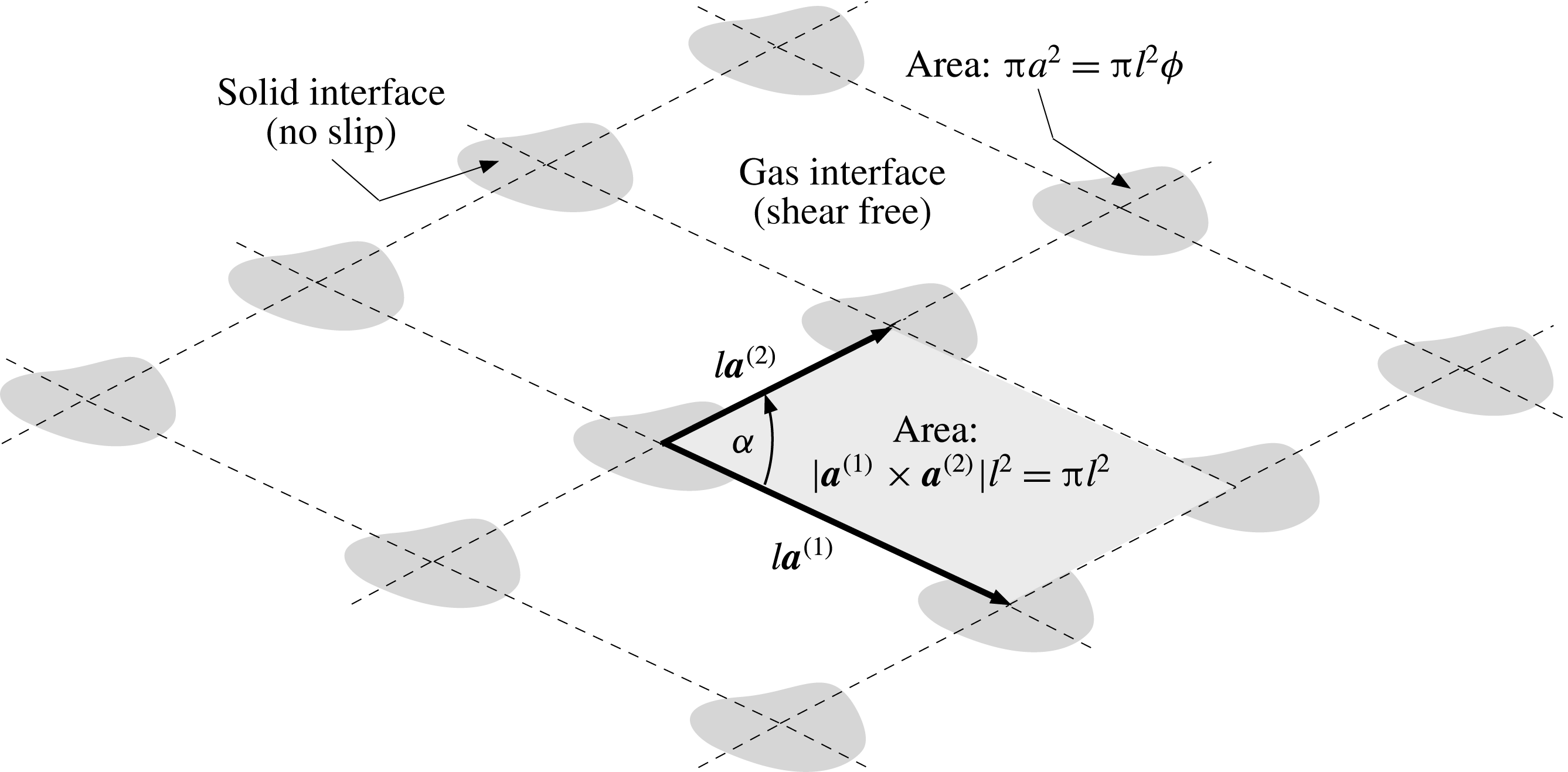
The periodic structure we consider is an array of identical pillars whose cross-sectional shape is arbitrary. The pillars are positioned about the vertices of a two-dimensional Bravais lattice (Kittel Reference Kittel2005). It is assumed that, upon submerging the array in liquid, air is trapped in between that liquid, the pillars and the solid substrate from which they protrude. A compound surface, consisting of the union of the top edges of the pillars and the liquid–air interface spanned between them, is accordingly formed. We restrict the analysis to the case of a flat compound surface.
Denoting the pillar cross-sectional area by
 $\unicode[STIX]{x03C0}a^{2}$
and the solid fraction of the superhydrophobic surface by
 $\unicode[STIX]{x1D719}$
, this surface is characterised by two length scales:
 $a$
, a representative dimension of the pillar cross-section, and
 $l=a\unicode[STIX]{x1D719}^{-1/2}$
, a linear dimension of the lattice cell. Employing
 $l$
as a length unit, we employ the Cartesian coordinates
 $(x,y,z)$
where the
 $xy$
-plane coincides with superhydrophobic surface. With no loss of generality, the
 $z$
-axis is assumed to pass through one of the pillars. The orientation of the
 $xy$
-axes relative to the lattice is not specified at this point.
The lattice is specified by two arbitrary (non-parallel) base vectors in the plane, say
 $\boldsymbol{a}^{(1)}$
and
 $\boldsymbol{a}^{(2)}$
. The vertices are accordingly located at
 $$\begin{eqnarray}\boldsymbol{r}=n_{1}\boldsymbol{a}^{(1)}+n_{2}\boldsymbol{a}^{(2)},\quad n_{1},n_{2}\in \mathbb{Z}.\end{eqnarray}$$
Since the number of pillars and cells is the same, the solid fraction
 $\unicode[STIX]{x1D719}$
corresponds to a dimensionless cell area
 $$\begin{eqnarray}A=|\boldsymbol{a}^{(1)}\boldsymbol{\times }\boldsymbol{a}^{(2)}|=\unicode[STIX]{x03C0}.\end{eqnarray}$$
The reciprocal lattice (Kittel Reference Kittel2005) is defined using the base vectors
 $$\begin{eqnarray}\boldsymbol{b}^{(1)}=\frac{2\unicode[STIX]{x03C0}}{A}\boldsymbol{a}^{(2)}\boldsymbol{\times }\hat{\boldsymbol{e}}_{z},\quad \boldsymbol{b}^{(2)}=\frac{2\unicode[STIX]{x03C0}}{A}\hat{\boldsymbol{e}}_{z}\boldsymbol{\times }\boldsymbol{a}^{(1)}.\end{eqnarray}$$
The vertices of that lattice are located at
 $$\begin{eqnarray}\boldsymbol{k}=n_{1}\boldsymbol{b}^{(1)}+n_{2}\boldsymbol{b}^{(2)},\quad n_{1},n_{2}\in \mathbb{Z}.\end{eqnarray}$$
The dimensional geometry of the superhydrophobic surface is portrayed in figure 1.
Dimensional schematic of the superhydrophobic surface (viewed from above). The imposed shear is applied in an arbitrary direction in the plane.

3 Problem formulation
A shear flow of rate
 $G$
is imposed at large distances from the surface in a direction specified by the unit vector
 $\hat{\boldsymbol{e}}$
. Following Davis & Lauga (Reference Davis and Lauga2010), we assume that the Reynolds number is small and that the free surface remains flat. We employ a dimensionless notation, normalising length variables by
 $l$
, velocities by
 $Gl$
and stresses by
 $\unicode[STIX]{x1D707}G$
,
 $\unicode[STIX]{x1D707}$
being the liquid viscosity.
The velocity
 $\boldsymbol{u}$
and pressure
 $p$
are governed by (i) the continuity and Stokes equations,
 $$\begin{eqnarray}\unicode[STIX]{x1D735}\boldsymbol{\cdot }\boldsymbol{u}=0,\quad \unicode[STIX]{x1D6FB}^{2}\boldsymbol{u}=\unicode[STIX]{x1D735}p;\end{eqnarray}$$
(ii) conditions at
 $z=0$
, consisting of no slip on the solid patches,
 $$\begin{eqnarray}\boldsymbol{u}=\mathbf{0},\end{eqnarray}$$
and impermeability and no shear on the free surface,
 $$\begin{eqnarray}\hat{\boldsymbol{e}}_{z}\boldsymbol{\cdot }\boldsymbol{u}=0,\quad (\unicode[STIX]{x1D644}-\hat{\boldsymbol{e}}_{z}\hat{\boldsymbol{e}}_{z})\boldsymbol{\cdot }\frac{\unicode[STIX]{x2202}\boldsymbol{u}}{\unicode[STIX]{x2202}z}=\mathbf{0}\end{eqnarray}$$
(
 $\unicode[STIX]{x1D644}$
being the unit tensor); and (iii) imposed shear at large distances (cf. (1.1))
 $$\begin{eqnarray}\boldsymbol{u}\sim z\hat{\boldsymbol{e}}\quad \text{as}~z\rightarrow \infty .\end{eqnarray}$$
The far-field asymptotic behaviour (3.4) may be refined to (cf. (1.2)–(1.3))
 $$\begin{eqnarray}\boldsymbol{u}\sim z\hat{\boldsymbol{e}}+\unicode[STIX]{x1D63D}\boldsymbol{\cdot }\hat{\boldsymbol{e}}+o(1)\quad \text{as}~z\rightarrow \infty .\end{eqnarray}$$
Our interest is in the slip-length tensor
 $\unicode[STIX]{x1D63D}$
. Note that this dimensionless object is a pure geometric quantity, and as such may only depend upon the solid fraction
 $\unicode[STIX]{x1D719}$
, the cross-sectional shape and the lattice geometry. While the flow problem (and hence
 $\unicode[STIX]{x1D63D}$
) is completely determined by (3.1)–(3.4), it is convenient to derive an integral constraint that relates the imposed shear to conditions applying over the solid patches. This constraint follows from an integral force balance. Thus, the shear flow is associated with a shear force (per unit area) of unit magnitude, applied at large
 $z$
in the
 $\hat{\boldsymbol{e}}$
-direction. In view of the shear-free condition (3.3b
), this force can only be supported by the solid pillars. Since one pillar is included in each lattice cell (of area
 $\unicode[STIX]{x03C0}$
) there are
 $1/\unicode[STIX]{x03C0}$
pillars per unit area. By symmetry, the force on each pillar is identical, namely
 $\unicode[STIX]{x03C0}\hat{\boldsymbol{e}}$
. To specify this force it suffices to consider a single ‘test’ pillar, say that centred about the origin,
 $$\begin{eqnarray}\iint \,\text{d}x\,\text{d}y\,(\unicode[STIX]{x1D644}-\hat{\boldsymbol{e}}_{z}\hat{\boldsymbol{e}}_{z})\boldsymbol{\cdot }\frac{\unicode[STIX]{x2202}\boldsymbol{u}}{\unicode[STIX]{x2202}z}=\unicode[STIX]{x03C0}\hat{\boldsymbol{e}}.\end{eqnarray}$$
Here, the integration is carried out over the cross-section (of area
 $\unicode[STIX]{x03C0}\unicode[STIX]{x1D719}$
) of that pillar. Being a consequence of the governing equations, relation (3.6) does not provide any independent information beyond that contained in (3.1)–(3.4). Nonetheless, it facilitates the subsequent investigation of the small-solid-fraction limit, both in the identification of the asymptotic scaling and the ensuing asymptotic analysis.
In what follows, it is convenient to define the ‘shifted’ velocity,
 $$\begin{eqnarray}\boldsymbol{u}^{\prime }=\boldsymbol{u}-z\hat{\boldsymbol{e}}-\unicode[STIX]{x1D63D}\boldsymbol{\cdot }\hat{\boldsymbol{e}},\end{eqnarray}$$
which, in view of (3.5), decays at large distances away from the surface,
 $$\begin{eqnarray}\boldsymbol{u}^{\prime }\rightarrow \mathbf{0}\quad \text{as}~z\rightarrow \infty .\end{eqnarray}$$
This field is also governed by the homogeneous continuity and Stokes equations (with the same pressure)
 $$\begin{eqnarray}\unicode[STIX]{x1D735}\boldsymbol{\cdot }\boldsymbol{u}^{\prime }=0,\quad \unicode[STIX]{x1D6FB}^{2}\boldsymbol{u}^{\prime }=\unicode[STIX]{x1D735}p.\end{eqnarray}$$
At
 $z=0$
it satisfies the slip condition on the solid patches,
 $$\begin{eqnarray}\boldsymbol{u}^{\prime }=-\unicode[STIX]{x1D63D}\boldsymbol{\cdot }\hat{\boldsymbol{e}},\end{eqnarray}$$
and the following conditions on the free surface,
 $$\begin{eqnarray}\hat{\boldsymbol{e}}_{z}\boldsymbol{\cdot }\boldsymbol{u}^{\prime }=0,\quad (\unicode[STIX]{x1D644}-\hat{\boldsymbol{e}}_{z}\hat{\boldsymbol{e}}_{z})\boldsymbol{\cdot }\frac{\unicode[STIX]{x2202}\boldsymbol{u}^{\prime }}{\unicode[STIX]{x2202}z}=-\hat{\boldsymbol{e}}.\end{eqnarray}$$
In terms of the shifted velocity, constraint (3.6) reads
 $$\begin{eqnarray}\iint \,\text{d}x\,\text{d}y\,(\unicode[STIX]{x1D644}-\hat{\boldsymbol{e}}_{z}\hat{\boldsymbol{e}}_{z})\boldsymbol{\cdot }\frac{\unicode[STIX]{x2202}\boldsymbol{u}^{\prime }}{\unicode[STIX]{x2202}z}=\unicode[STIX]{x03C0}(1-\unicode[STIX]{x1D719})\hat{\boldsymbol{e}}.\end{eqnarray}$$
4 Small solid fractions
We now consider the asymptotic limit
 $\unicode[STIX]{x1D719}\ll 1$
. This singular limit is handled using matched asymptotic expansions, with separate expansions holding in an outer region, which corresponds to the limit
 $\unicode[STIX]{x1D719}\rightarrow 0$
with
 $\boldsymbol{x}$
fixed (
 $\boldsymbol{x}$
being the position vector), and an inner region of
 $\unicode[STIX]{x1D719}^{1/2}$
extent, which corresponds to the limit
 $\unicode[STIX]{x1D719}\rightarrow 0$
with
 $\boldsymbol{X}=\unicode[STIX]{x1D719}^{-1/2}\boldsymbol{x}$
fixed.
In the outer region, where at leading order the solid patches at
 $z=0$
appear as points, the shifted velocity field
 $\boldsymbol{u}^{\prime }$
satisfies the continuity and Stokes equations and large-
 $z$
decay. The free-surface conditions (3.11) now apply at the punctured
 $z=0$
plane, while the slip condition (3.10) does not apply in that region. Note that condition (3.11b
) implies that
 $\boldsymbol{u}^{\prime }$
is
 $O(1)$
in the outer region. We accordingly apply the following outer expansion,
 $$\begin{eqnarray}\boldsymbol{u}^{\prime }(\boldsymbol{x};\unicode[STIX]{x1D719})=\boldsymbol{u}_{0}^{\prime }(\boldsymbol{x})+\unicode[STIX]{x1D719}^{1/2}\boldsymbol{u}_{1/2}^{\prime }(\boldsymbol{x})+\cdots \,,\end{eqnarray}$$
with a similar expansion of
 $p$
.
The inner region is described by the stretched coordinates of
 $\boldsymbol{X}$
, say
 $(X,Y,Z)$
. These correspond to normalisation by
 $a$
. From (3.12) it is evident that
 $\boldsymbol{u}^{\prime }$
is of order
 $\unicode[STIX]{x1D719}^{-1/2}$
in that region, whereby the Stokes equations (3.9) imply that
 $p$
is of order
 $\unicode[STIX]{x1D719}^{-1}$
there. The rescaled velocity
 $\boldsymbol{U}$
and pressure
 $P$
, defined by
 $$\begin{eqnarray}\boldsymbol{u}^{\prime }=\unicode[STIX]{x1D719}^{-1/2}\boldsymbol{U},\quad p=\unicode[STIX]{x1D719}^{-1}P,\end{eqnarray}$$
are accordingly
 $O(1)$
in the inner region. The
 $O(\unicode[STIX]{x1D719}^{-1/2})$
scaling of
 $\boldsymbol{u}^{\prime }$
in the inner region also implies, through the slip condition (3.10), that
 $\unicode[STIX]{x1D63D}$
has the same scaling (see (4.8)). The preceding asymptotic estimates constitute the dimensionless counterpart of the scaling arguments of Ybert et al. (Reference Ybert, Barentin, Cottin-Bizonne, Joseph and Bocquet2007).
In what follows we outline the problem satisfied by the inner flow
 $\boldsymbol{U}$
. It is governed by the Stokes equations,
 $$\begin{eqnarray}\unicode[STIX]{x1D735}_{\boldsymbol{X}}\boldsymbol{\cdot }\boldsymbol{U}=0,\quad \unicode[STIX]{x1D6FB}_{\boldsymbol{X}}^{2}\boldsymbol{U}=\unicode[STIX]{x1D735}_{\boldsymbol{ X}}P,\end{eqnarray}$$
wherein
 $\unicode[STIX]{x1D735}_{\boldsymbol{X}}=\hat{\boldsymbol{e}}_{x}\unicode[STIX]{x2202}/\unicode[STIX]{x2202}X+\hat{\boldsymbol{e}}_{y}\unicode[STIX]{x2202}/\unicode[STIX]{x2202}Y+\hat{\boldsymbol{e}}_{z}\unicode[STIX]{x2202}/\unicode[STIX]{x2202}Z$
is the stretched gradient operator. At
 $Z=0$
it satisfies the slip condition on the solid patches (cf. (3.10)),
 $$\begin{eqnarray}\boldsymbol{U}=-\unicode[STIX]{x1D719}^{1/2}\unicode[STIX]{x1D63D}\boldsymbol{\cdot }\hat{\boldsymbol{e}},\end{eqnarray}$$
while at the free surface (3.11) gives
 $$\begin{eqnarray}\hat{\boldsymbol{e}}_{z}\boldsymbol{\cdot }\boldsymbol{U}=0,\quad (\unicode[STIX]{x1D644}-\hat{\boldsymbol{e}}_{z}\hat{\boldsymbol{e}}_{z})\boldsymbol{\cdot }\frac{\unicode[STIX]{x2202}\boldsymbol{U}}{\unicode[STIX]{x2202}Z}=-\unicode[STIX]{x1D719}\hat{\boldsymbol{e}}.\end{eqnarray}$$
Note that the far-field condition (3.8) does not apply in the inner region. Rather, at large
 $|\boldsymbol{X}|$
the inner flow must match the outer one. On the other hand, the force constraint (3.12) does apply in the inner region, giving
 $$\begin{eqnarray}\iint \,\text{d}X\,\text{d}Y(\unicode[STIX]{x1D644}-\hat{\boldsymbol{e}}_{z}\hat{\boldsymbol{e}}_{z})\boldsymbol{\cdot }\frac{\unicode[STIX]{x2202}\boldsymbol{U}}{\unicode[STIX]{x2202}Z}=(\unicode[STIX]{x03C0}-\unicode[STIX]{x1D719})\hat{\boldsymbol{e}},\end{eqnarray}$$
where the integration is carried out over the cross-section of the single test pillar (whose area in terms of the inner coordinates is
 $\unicode[STIX]{x03C0}$
). As this condition represents the applied shear, it may serve as a convenient alternative to asymptotic matching, and may thus be considered as independent.
Analogously to (4.1) we employ the outer expansion,
 $$\begin{eqnarray}\boldsymbol{U}(\boldsymbol{X};\unicode[STIX]{x1D719})=\boldsymbol{U}_{0}(\boldsymbol{X})+\unicode[STIX]{x1D719}^{1/2}\boldsymbol{U}_{1/2}(\boldsymbol{X})+\cdots \,,\end{eqnarray}$$
with a similar one of
 $P$
. The corresponding expansion for
 $\unicode[STIX]{x1D63D}$
is (see (4.4))
 $$\begin{eqnarray}\unicode[STIX]{x1D63D}=\unicode[STIX]{x1D719}^{-1/2}\unicode[STIX]{x1D63D}_{-1/2}+\unicode[STIX]{x1D63D}_{0}+\cdots \,.\end{eqnarray}$$
5 Leading-order inner analysis and
 $O(\unicode[STIX]{x1D719}^{-1/2})$
slip length

Consider first the
 $O(\unicode[STIX]{x1D719}^{-1/2})$
inner velocity
 $\boldsymbol{U}_{0}$
. In the upper-half space
 $Z>0$
it is governed by the continuity and Stokes equations,
 $$\begin{eqnarray}\unicode[STIX]{x1D735}_{\boldsymbol{X}}\boldsymbol{\cdot }\boldsymbol{U}_{0}=0,\quad \unicode[STIX]{x1D6FB}_{\boldsymbol{X}}^{2}\boldsymbol{U}_{0}=\unicode[STIX]{x1D735}_{\boldsymbol{X}}P_{0}.\end{eqnarray}$$
At
 $Z=0$
it satisfies a slip condition at the solid interface,
 $$\begin{eqnarray}\boldsymbol{U}_{0}=-\unicode[STIX]{x1D63D}_{-1/2}\boldsymbol{\cdot }\hat{\boldsymbol{e}},\end{eqnarray}$$
and a shear-free condition at the gas interface,
 $$\begin{eqnarray}\hat{\boldsymbol{e}}_{z}\boldsymbol{\cdot }\boldsymbol{U}_{0}=0,\quad (\unicode[STIX]{x1D644}-\hat{\boldsymbol{e}}_{z}\hat{\boldsymbol{e}}_{z})\boldsymbol{\cdot }\frac{\unicode[STIX]{x2202}\boldsymbol{U}_{0}}{\unicode[STIX]{x2202}Z}=0.\end{eqnarray}$$
Finally, with the outer velocity
 $\boldsymbol{u}^{\prime }$
being
 $O(1)$
,
 $1$
–
 $1$
Van Dyke matching (Hinch Reference Hinch1991) implies the decay condition,
 $$\begin{eqnarray}\boldsymbol{U}_{0}\rightarrow \mathbf{0}\quad \text{as}~|\boldsymbol{X}|\rightarrow \infty .\end{eqnarray}$$
The above problem is supplemented by the constraint (cf. (4.6))
 $$\begin{eqnarray}\iint \,\text{d}X~\text{d}Y(\unicode[STIX]{x1D644}-\hat{\boldsymbol{e}}_{z}\hat{\boldsymbol{e}}_{z})\boldsymbol{\cdot }\frac{\unicode[STIX]{x2202}\boldsymbol{U}_{0}}{\unicode[STIX]{x2202}Z}=\unicode[STIX]{x03C0}\hat{\boldsymbol{e}}.\end{eqnarray}$$
Forming an even extension of the above problem about the plane
 $Z=0$
reveals that it is identical to that governing the flow about a flat disk, of the same shape as that of the pillar cross-section, which translates in its plane with velocity (normalised by
 $\unicode[STIX]{x1D719}^{-1/2}lG$
)
 $-\unicode[STIX]{x1D63D}_{-1/2}\boldsymbol{\cdot }\hat{\boldsymbol{e}}$
and does not rotate, while experiencing a hydrodynamic force (normalised by
 $\unicode[STIX]{x1D707}l^{2}G$
)
 $2\unicode[STIX]{x03C0}\hat{\boldsymbol{e}}$
. Since
 $\hat{\boldsymbol{e}}$
is arbitrary in the plane, we find
 $$\begin{eqnarray}\unicode[STIX]{x1D63D}_{-1/2}=2\unicode[STIX]{x03C0}\unicode[STIX]{x1D64D}^{-1},\end{eqnarray}$$
where
 $\unicode[STIX]{x1D64D}$
is the resistance tensor of the disk in the
 $xy$
-plane (normalised by
 $\unicode[STIX]{x1D707}a$
). Note that
 $\unicode[STIX]{x1D64D}^{-1}$
generally does not represent a mobility tensor in the
 $xy$
-plane, since the latter is affected by the coupling tensor.
For the case of circular pillars we may use the known resistance (Lamb Reference Lamb1945, article 339) of a flat circular disk translating broadside-on,
 $\unicode[STIX]{x1D64D}=(32/3)(\hat{\boldsymbol{e}}_{x}\hat{\boldsymbol{e}}_{x}+\hat{\boldsymbol{e}}_{y}\hat{\boldsymbol{e}}_{y})$
. This yields
 $$\begin{eqnarray}\unicode[STIX]{x1D63D}_{-1/2}=\frac{3\unicode[STIX]{x03C0}}{16}(\hat{\boldsymbol{e}}_{x}\hat{\boldsymbol{e}}_{x}+\hat{\boldsymbol{e}}_{y}\hat{\boldsymbol{e}}_{y}),\end{eqnarray}$$
in agreement with Davis & Lauga (Reference Davis and Lauga2010). (Notice that Davis & Lauga (Reference Davis and Lauga2010) obtained that value for the particular case of a rectangular lattice, while our analysis reveals its applicability to arbitrary Bravais lattices.) The anisotropic case of elliptic cross-section is described in appendix A.
Towards subsequent evaluation of the outer flow we note that the asymptotic form taken by
 $\boldsymbol{U}_{0}$
at large
 $|\boldsymbol{X}|$
is independent of the cross-sectional shape. Thus, consistently with (5.5) we find that
 $$\begin{eqnarray}\boldsymbol{U}_{0}\sim -\frac{1}{4}\hat{\boldsymbol{e}}\boldsymbol{\cdot }\left(\frac{\unicode[STIX]{x1D644}}{|\boldsymbol{X}|}+\frac{\boldsymbol{X}\boldsymbol{X}}{|\boldsymbol{X}|^{3}}\right),\end{eqnarray}$$
representing a concentrated force
 $-2\unicode[STIX]{x03C0}\hat{\boldsymbol{e}}$
acting on the liquid.
6 Leading-order outer analysis
Consider
 $\boldsymbol{u}_{0}^{\prime }$
, the leading-order shifted flow in the outer region. It is governed by the Stokes equations, attenuation at infinity, and the free-surface conditions,
 $$\begin{eqnarray}\hat{\boldsymbol{e}}_{z}\boldsymbol{\cdot }\boldsymbol{u}_{0}^{\prime }=0,\quad (\unicode[STIX]{x1D644}-\hat{\boldsymbol{e}}_{z}\hat{\boldsymbol{e}}_{z})\boldsymbol{\cdot }\frac{\unicode[STIX]{x2202}\boldsymbol{u}_{0}^{\prime }}{\unicode[STIX]{x2202}z}=-\hat{\boldsymbol{e}},\end{eqnarray}$$
at the punctured
 $z=0$
plane. In addition,
 $2$
–
 $1$
Van Dyke matching implies that
 $$\begin{eqnarray}\boldsymbol{u}_{0}^{\prime }\sim -\frac{1}{4}\hat{\boldsymbol{e}}\boldsymbol{\cdot }\left(\frac{\unicode[STIX]{x1D644}}{|\boldsymbol{x}|}+\frac{\boldsymbol{x}\boldsymbol{x}}{|\boldsymbol{x}|^{3}}\right)\quad \text{as}~\boldsymbol{x}\rightarrow \mathbf{0}.\end{eqnarray}$$
It follows that
 $\boldsymbol{u}_{0}^{\prime }$
consists of (i) a two-dimensional array of identical Stokeslets of magnitude
 $-2\unicode[STIX]{x03C0}\hat{\boldsymbol{e}}$
, positioned at the lattice vertices; and (ii) the additional flow required to create the opposing shear at
 $z=0$
. An analogous flow problem was solved by Pozrikidis (Reference Pozrikidis1996) using the Fourier series solution of Hasimoto (Reference Hasimoto1959). In the present dimensionless notation we find that
 $$\begin{eqnarray}\boldsymbol{u}_{0}^{\prime }=\hat{\boldsymbol{e}}\boldsymbol{\cdot }\mathop{\sum }_{\boldsymbol{k}\neq \mathbf{0}}\left(\unicode[STIX]{x1D644}\unicode[STIX]{x1D6FB}^{2}-\unicode[STIX]{x1D735}\unicode[STIX]{x1D735}\right)S,\end{eqnarray}$$
where
 $\boldsymbol{k}$
is a point on the reciprocal lattice, of the form (2.4), and
 $$\begin{eqnarray}S=\frac{1+kz}{2k^{3}}\exp (-\text{i}\boldsymbol{k}\boldsymbol{\cdot }\boldsymbol{x}-kz),\end{eqnarray}$$
in which
 $k=|\boldsymbol{k}|$
.
7
$O(1)$
inner flow and slip length

Consider now the
 $O(1)$
inner velocity
 $\boldsymbol{U}_{1/2}$
. It is governed by (i) the continuity and Stokes equations,
 $$\begin{eqnarray}\unicode[STIX]{x1D735}_{\boldsymbol{X}}\boldsymbol{\cdot }\boldsymbol{U}_{1/2}=0,\quad \unicode[STIX]{x1D6FB}_{\boldsymbol{X}}^{2}\boldsymbol{U}_{1/2}=\unicode[STIX]{x1D735}_{\boldsymbol{X}}P_{1/2};\end{eqnarray}$$
(ii) conditions at
 $Z=0$
, consisting of a slip condition on the solid portion,
 $$\begin{eqnarray}\boldsymbol{U}_{1/2}=-\unicode[STIX]{x1D63D}_{0}\boldsymbol{\cdot }\hat{\boldsymbol{e}},\end{eqnarray}$$
and a shear-free condition at the free surface,
 $$\begin{eqnarray}\hat{\boldsymbol{e}}_{z}\boldsymbol{\cdot }\boldsymbol{U}_{1/2}=0,\quad (\unicode[STIX]{x1D644}-\hat{\boldsymbol{e}}_{z}\hat{\boldsymbol{e}}_{z})\boldsymbol{\cdot }\frac{\unicode[STIX]{x2202}\boldsymbol{U}_{1/2}}{\unicode[STIX]{x2202}Z}=0;\end{eqnarray}$$
and (iii) the constraint (cf. (4.6))
 $$\begin{eqnarray}\iint \,\text{d}X\,\text{d}Y(\unicode[STIX]{x1D644}-\hat{\boldsymbol{e}}_{z}\hat{\boldsymbol{e}}_{z})\boldsymbol{\cdot }\frac{\unicode[STIX]{x2202}\boldsymbol{U}_{1/2}}{\unicode[STIX]{x2202}Z}=\mathbf{0}.\end{eqnarray}$$
Since both the shear-stress condition (4.5b
) and force constraint (4.6) are trivial at
 $O(\unicode[STIX]{x1D719}^{1/2})$
, the only inhomogeneous equation in the above problem is (7.2). It is then readily seen that the uniform flow,
 $$\begin{eqnarray}\boldsymbol{U}_{1/2}\equiv -\unicode[STIX]{x1D63D}_{0}\boldsymbol{\cdot }\hat{\boldsymbol{e}},\end{eqnarray}$$
trivially satisfies this problem.
To obtain
 $\unicode[STIX]{x1D63D}_{0}$
we now employ
 $2$
–
 $2$
Van Dyke matching. Thus, making use of (5.8) and (7.5) we find
 $$\begin{eqnarray}\boldsymbol{u}_{0}^{\prime }\sim -\frac{1}{4}\hat{\boldsymbol{e}}\boldsymbol{\cdot }\left(\frac{\unicode[STIX]{x1D644}}{|\boldsymbol{x}|}+\frac{\boldsymbol{x}\boldsymbol{x}}{|\boldsymbol{x}|^{3}}\right)-\unicode[STIX]{x1D63D}_{0}\boldsymbol{\cdot }\hat{\boldsymbol{e}}\quad \text{as}~\boldsymbol{x}\rightarrow \mathbf{0}.\end{eqnarray}$$
Substitution of (6.3) gives
 $$\begin{eqnarray}\unicode[STIX]{x1D63D}_{0}\boldsymbol{\cdot }\hat{\boldsymbol{e}}=\hat{\boldsymbol{e}}\boldsymbol{\cdot }\lim _{\boldsymbol{x}\rightarrow \mathbf{0}}\left[\mathop{\sum }_{\boldsymbol{k}\neq \mathbf{0}}\left(\unicode[STIX]{x1D735}\unicode[STIX]{x1D735}-\unicode[STIX]{x1D644}\unicode[STIX]{x1D6FB}^{2}\right)S-\frac{1}{4}\left(\frac{\unicode[STIX]{x1D644}}{|\boldsymbol{x}|}+\frac{\boldsymbol{x}\boldsymbol{x}}{|\boldsymbol{x}|^{3}}\right)\right].\end{eqnarray}$$
At this stage it is convenient to express
 $\unicode[STIX]{x1D63D}_{0}$
in terms of its components in (arbitrary) Cartesian
 $xy$
-coordinates, say,
 $$\begin{eqnarray}\unicode[STIX]{x1D63D}_{0}=B_{xx}\hat{\boldsymbol{e}}_{x}\hat{\boldsymbol{e}}_{x}+B_{yy}\hat{\boldsymbol{e}}_{y}\hat{\boldsymbol{e}}_{y}+B_{xy}\hat{\boldsymbol{e}}_{x}\hat{\boldsymbol{e}}_{y}+B_{yx}\hat{\boldsymbol{e}}_{y}\hat{\boldsymbol{e}}_{x}.\end{eqnarray}$$
Since
 $\hat{\boldsymbol{e}}$
is an arbitrary unit vector in the
 $xy$
plane, we find from (7.7)
 $$\begin{eqnarray}\displaystyle & \displaystyle B_{xx}=-\lim _{\boldsymbol{x}\rightarrow \mathbf{0}}\left[\mathop{\sum }_{\boldsymbol{k}\neq \mathbf{0}}\left(\frac{\unicode[STIX]{x2202}^{2}S}{\unicode[STIX]{x2202}y^{2}}+\frac{\unicode[STIX]{x2202}^{2}S}{\unicode[STIX]{x2202}z^{2}}\right)+\frac{|\boldsymbol{x}|^{2}+x^{2}}{4|\boldsymbol{x}|^{3}}\right], & \displaystyle\end{eqnarray}$$
 $$\begin{eqnarray}\displaystyle & \displaystyle B_{yy}=-\lim _{\boldsymbol{x}\rightarrow \mathbf{0}}\left[\mathop{\sum }_{\boldsymbol{k}\neq \mathbf{0}}\left(\frac{\unicode[STIX]{x2202}^{2}S}{\unicode[STIX]{x2202}x^{2}}+\frac{\unicode[STIX]{x2202}^{2}S}{\unicode[STIX]{x2202}z^{2}}\right)+\frac{|\boldsymbol{x}|^{2}+y^{2}}{4|\boldsymbol{x}|^{3}}\right], & \displaystyle\end{eqnarray}$$
and
 $$\begin{eqnarray}B_{xy}=B_{yx}=\lim _{\boldsymbol{x}\rightarrow \mathbf{0}}\left[\mathop{\sum }_{\boldsymbol{k}\neq \mathbf{0}}\frac{\unicode[STIX]{x2202}^{2}S}{\unicode[STIX]{x2202}x\,\unicode[STIX]{x2202}y}-\frac{xy}{4|\boldsymbol{x}|^{3}}\right].\end{eqnarray}$$
Note that
 $\unicode[STIX]{x1D63D}_{0}$
is independent of the pillar cross-sectional shape. This may be traced to the far-field Stokeslet behaviour (5.8) which is independent of that shape.
8 Calculation of
$B_{xx}$
,
$B_{yy}$
and
$B_{xy}$


Expressions (7.9)–(7.11) provide the requisite components of the slip-length tensor at
 $O(1)$
as functions of the lattice geometry. Since these are expressed in terms of certain limits, they should be viewed as formal expressions. In this section we obtain operative expressions for the above components.
Recall that the orientation of the
 $xy$
-axes relative to the lattice is arbitrary. The expression for
 $B_{yy}$
may therefore be readily inferred from that of
 $B_{xx}$
. It is accordingly sufficient to consider
 $B_{xx}$
and
 $B_{xy}$
. We start with substitution of (6.4) into (7.9) and (7.11), giving
 $$\begin{eqnarray}\displaystyle & \displaystyle B_{xx}=\lim _{\boldsymbol{x}\rightarrow \mathbf{0}}\left[\mathop{\sum }_{\boldsymbol{k}\neq \mathbf{0}}\frac{k_{y}^{2}+k^{2}-k_{x}^{2}kz}{2k^{3}}\text{e}^{-\text{i}\boldsymbol{k}\boldsymbol{\cdot }\boldsymbol{x}-kz}-\frac{|\boldsymbol{x}|^{2}+x^{2}}{4|\boldsymbol{x}|^{3}}\right], & \displaystyle\end{eqnarray}$$
 $$\begin{eqnarray}\displaystyle & \displaystyle B_{xy}=\lim _{\boldsymbol{x}\rightarrow \mathbf{0}}\left[\mathop{\sum }_{\boldsymbol{k}\neq \mathbf{0}}\frac{k_{x}k_{y}(1+kz)}{4k^{3}}\text{e}^{-\text{i}\boldsymbol{k}\boldsymbol{\cdot }\boldsymbol{x}-kz}+\frac{xy}{4|\boldsymbol{x}|^{3}}\right]. & \displaystyle\end{eqnarray}$$
Since the limits attained as
 $\boldsymbol{x}\rightarrow \mathbf{0}$
must be independent of the manner by which the origin is approached, we may set
 $y=z=0$
(so that
 $\boldsymbol{x}=\hat{\boldsymbol{e}}_{x}x$
) and assume
 $x>0$
. We then obtain
 $$\begin{eqnarray}\displaystyle & \displaystyle B_{xx}=\frac{1}{2}\lim _{x\rightarrow 0^{+}}\left(\mathop{\sum }_{\boldsymbol{k}\neq \mathbf{0}}\frac{k_{y}^{2}+k^{2}}{k^{3}}\text{e}^{-\text{i}\boldsymbol{k}\boldsymbol{\cdot }\hat{\boldsymbol{e}}_{x}x}-\frac{1}{x}\right), & \displaystyle\end{eqnarray}$$
 $$\begin{eqnarray}\displaystyle & \displaystyle B_{xy}=-\frac{1}{2}\lim _{x\rightarrow 0^{+}}\mathop{\sum }_{\boldsymbol{k}\neq \mathbf{0}}\frac{k_{x}k_{y}}{k^{3}}\text{e}^{-\text{i}\boldsymbol{k}\boldsymbol{\cdot }\hat{\boldsymbol{e}}_{x}x}. & \displaystyle\end{eqnarray}$$
In (8.4) we may simply apply the limit term by term, providing the result
 $$\begin{eqnarray}B_{xy}=-\frac{1}{2}\mathop{\sum }_{\boldsymbol{k}\neq \mathbf{0}}\frac{k_{x}k_{y}}{k^{3}}.\end{eqnarray}$$
No such interchange is possible in the first term of (8.3), since the lattice sum of
 $1/k$
does not converge. This is of course evident from the need to produce a singular term that would cancel out the
 $1/x$
term in (8.3). We accordingly need to produce a two-term asymptotic expansion of the lattice sum appearing in (8.3).
The method for accomplishing that is based upon the introduction of a function
 ${\mathcal{F}}(k)$
which (i) decays at an exponential rate at large
 $k$
; and (ii) satisfies
 $$\begin{eqnarray}1-{\mathcal{F}}(k)=o(k)\quad \text{as}~k\rightarrow 0.\end{eqnarray}$$
Otherwise, it is arbitrary. (While the requirement of exponential decay can be somewhat relaxed, we see no real need for extending the present arbitrariness. There is no problem in identifying appropriate functions which satisfy stipulations (i) and (ii): see e.g. (8.13).) Making use of that function we show in appendix B that
 $$\begin{eqnarray}\mathop{\sum }_{\boldsymbol{k}\neq 0}\frac{k_{y}^{2}+k^{2}}{k^{3}}\text{e}^{-\text{i}\boldsymbol{k}\boldsymbol{\cdot }\hat{\boldsymbol{e}}_{x}x}\sim \frac{1}{x}+{\mathcal{C}}+o(1)\quad \text{as}~x\rightarrow 0^{+},\end{eqnarray}$$
in which
 $$\begin{eqnarray}{\mathcal{C}}=-\frac{3}{4}\int _{0}^{\infty }{\mathcal{F}}(\unicode[STIX]{x1D714})\,\text{d}\unicode[STIX]{x1D714}+\frac{1}{4}\mathop{\sum }_{\boldsymbol{r}\neq \mathbf{0}}\left[3M_{0}(r)+M_{2}(r)\cos 2\unicode[STIX]{x1D703}\right]+\mathop{\sum }_{\boldsymbol{k}\neq \mathbf{0}}\frac{k_{y}^{2}+k^{2}}{k^{3}}{\mathcal{F}}(k),\end{eqnarray}$$
wherein
 $\boldsymbol{r}$
is a lattice point (of the form (2.1)) with polar coordinates
 $(r,\unicode[STIX]{x1D703})$
and the functions
 $M_{n}$
are defined in (B 14). Since
 ${\mathcal{C}}$
must be independent of the choice of
 ${\mathcal{F}}(k)$
, it depends only on the lattice geometry. Substitution of (8.7) into (8.3) yields the slip length
 $$\begin{eqnarray}B_{xx}={\textstyle \frac{1}{2}}{\mathcal{C}}.\end{eqnarray}$$
The slip length
 $B_{yy}$
may be obtained by calculating
 $B_{xx}$
with the lattice rotated
 $90^{\circ }$
in the clockwise direction (implying the same rotation of the reciprocal lattice). These rotations correspond to the transformations
 $$\begin{eqnarray}\unicode[STIX]{x1D703}\rightarrow \unicode[STIX]{x1D703}-\unicode[STIX]{x03C0}/2,\quad k_{x}\rightarrow k_{y},\quad k_{y}\rightarrow -k_{x}.\end{eqnarray}$$
Thus, defining
 $$\begin{eqnarray}\tilde{{\mathcal{C}}}=-\frac{3}{4}\int _{0}^{\infty }{\mathcal{F}}(\unicode[STIX]{x1D714})\,\text{d}\unicode[STIX]{x1D714}+\frac{1}{4}\mathop{\sum }_{\boldsymbol{r}\neq \mathbf{0}}\left[3M_{0}(r)-M_{2}(r)\cos 2\unicode[STIX]{x1D703}\right]+\mathop{\sum }_{\boldsymbol{k}\neq \mathbf{0}}\frac{k_{x}^{2}+k^{2}}{k^{3}}{\mathcal{F}}(k),\end{eqnarray}$$
we obtain
 $$\begin{eqnarray}B_{yy}={\textstyle \frac{1}{2}}\tilde{{\mathcal{C}}}.\end{eqnarray}$$
Formulae (8.5), (8.9) and (8.12) provide the
 $O(1)$
slip-length tensor for any lattice shape. In our subsequent calculations of these formulae we have made use of the special choice
 $$\begin{eqnarray}{\mathcal{F}}(k)=(1+k)\text{e}^{-k},\end{eqnarray}$$
which clearly satisfies (8.6). With that choice,
 $$\begin{eqnarray}\int _{0}^{\infty }{\mathcal{F}}(\unicode[STIX]{x1D714})\,\text{d}\unicode[STIX]{x1D714}=2,\quad M_{0}(r)=\frac{1}{r}-\frac{r^{2}+2}{(r^{2}+1)^{3/2}},\quad M_{2}(r)=\frac{1}{r}-\frac{r^{2}}{(r^{2}+1)^{3/2}}.\end{eqnarray}$$
Note that both
 $M_{0}$
and
 $M_{2}$
are
 $O(r^{-3})$
at large
 $r$
. The lattice sums appearing in (8.8) and (8.11) are absolutely convergent.
9 Discussion
We have derived small-solid-fraction approximations for the slip length
 $\unicode[STIX]{x1D740}$
of a generic micropillared superhydrophobic surface,
 $$\begin{eqnarray}\unicode[STIX]{x1D740}/l=\unicode[STIX]{x1D63D}\boldsymbol{\cdot }\hat{\boldsymbol{e}},\quad \unicode[STIX]{x1D63D}\sim \unicode[STIX]{x1D719}^{-1/2}\unicode[STIX]{x1D63D}_{-1/2}+\unicode[STIX]{x1D63D}_{0}+o(1),\end{eqnarray}$$
where
 $\unicode[STIX]{x1D719}\ll 1$
is the solid fraction,
 $\hat{\boldsymbol{e}}$
is a unit vector in the direction of the applied shear,
 $\unicode[STIX]{x1D63D}_{-1/2}$
and
 $\unicode[STIX]{x1D63D}_{0}$
are
 $\unicode[STIX]{x1D719}$
-independent dimensionless slip-length tensors and
 $l=L/\sqrt{\unicode[STIX]{x03C0}}$
,
 $L^{2}$
being the dimensional unit cell area. The leading-order term
 $\unicode[STIX]{x1D63D}_{-1/2}$
is found to be independent of the lattice geometry; it is related through (5.6) to the drag due to pure translation of a flattened disk shaped like the pillar cross-section. For circular pillars this analogy readily yields the scalar slip length (cf. (5.7))
 $$\begin{eqnarray}\frac{\unicode[STIX]{x1D706}}{L}\sim \frac{3\sqrt{\unicode[STIX]{x03C0}}}{16}\unicode[STIX]{x1D719}^{-1/2}+O(1),\end{eqnarray}$$
which agrees with the leading term in the expansion obtained by Davis & Lauga (Reference Davis and Lauga2010) for the special case of a rectangular lattice. As demonstrated by Davis & Lauga (Reference Davis and Lauga2010), this leading term is in good agreement with computations by Ybert et al. (Reference Ybert, Barentin, Cottin-Bizonne, Joseph and Bocquet2007) and Ng & Wang (Reference Ng and Wang2010). Surprisingly,
 $3\sqrt{\unicode[STIX]{x03C0}}/16$
is also close (to two per cent) to the value obtained for square pillars (Ng & Wang Reference Ng and Wang2010), suggesting that the drag on a translating square disk is close to that on a circular disk of the same area. (We are not aware of any Stokes flow calculation of the drag on the former.) In appendix A we derive explicit formulae for elliptical pillars, which could be used to realise large anisotropic slip lengths with tuneable principal directions and min-to-max slip-length ratios (up to two in the limit of slender ellipses).
The correction term
 $\unicode[STIX]{x1D63D}_{0}$
depends on the geometry of the lattice but not on the cross-sectional shape of the pillars. In § 8 we provide explicit formulae for calculating
 $\unicode[STIX]{x1D63D}_{0}$
in terms of its components
 $B_{xx},B_{yy}$
and
 $B_{xy}$
in an arbitrary Cartesian frame and for an arbitrary Bravais lattice. In our dimensionless formulation, where lengths are normalised by
 $l$
, that lattice is completely specified by the angle
 $\unicode[STIX]{x1D6FC}$
between the two base vectors
 $\boldsymbol{a}^{(1)}$
and
 $\boldsymbol{a}^{(2)}$
and the ratio
 $\unicode[STIX]{x1D712}$
of their magnitudes, the respective dimensionless lengths then being
 $\unicode[STIX]{x03C0}^{1/2}(\unicode[STIX]{x1D712}\sin \unicode[STIX]{x1D6FC})^{-1/2}$
and
 $(\unicode[STIX]{x03C0}\unicode[STIX]{x1D712})^{1/2}(\sin \unicode[STIX]{x1D6FC})^{-1/2}$
.
The case of a square lattice (
 $\unicode[STIX]{x1D712}=1,\unicode[STIX]{x1D6FC}=\unicode[STIX]{x03C0}/2$
) is of particular interest, given the availability of both numerical (Ybert et al.
Reference Ybert, Barentin, Cottin-Bizonne, Joseph and Bocquet2007; Ng & Wang Reference Ng and Wang2010) and analytic (Davis & Lauga Reference Davis and Lauga2010) results. In this case the tensor
 $\unicode[STIX]{x1D63D}_{0}$
is isotropic, with
 $B_{xx}=B_{yy}$
(as is indeed evident from (8.9) and (8.12)) and
 $B_{xy}=0$
(as is also evident from (8.5)). In calculating the two lattice sums appearing in (8.8) we conveniently choose the
 $x$
- and
 $y$
-axes in the directions of
 $\boldsymbol{a}^{(1)}$
and
 $\boldsymbol{a}^{(2)}$
, respectively. Since both sums are absolutely convergent, their evaluation does not impose any computational effort. Our calculation gives
 $B_{xx}=-0.8251$
. The scalar slip length, normalised by the lattice pitch
 $L$
, is thus
 $$\begin{eqnarray}\frac{\unicode[STIX]{x1D706}}{L}\sim \frac{3\sqrt{\unicode[STIX]{x03C0}}}{16}\unicode[STIX]{x1D719}^{-1/2}-B+o(1),\end{eqnarray}$$
where
 $$\begin{eqnarray}B=-\unicode[STIX]{x03C0}^{-1/2}B_{xx}=0.4655.\end{eqnarray}$$
Our value (9.4) is in excellent agreement (to approximately 0.5 %) with the value
 $B=0.468$
provided by Ng & Wang (Reference Ng and Wang2010); the latter value was determined by Ng & Wang (Reference Ng and Wang2010) via fitting their numerical simulations for circular pillars with a scaling law of the form (9.3). Curiously, the closed-form result derived by Davis & Lauga (Reference Davis and Lauga2010),
 $B=3\ln (1+\sqrt{2})/2\unicode[STIX]{x03C0}=0.4208$
, differs from the fitted value by approximately 10 %; with
 $B$
being a pure number, independent of
 $\unicode[STIX]{x1D719}$
, we find this twentyfold inaccuracy puzzling. Last, we note that Ng & Wang (Reference Ng and Wang2010) find
 $B=0.461$
when fitting their computations in the case of square pillars. The fact that our prediction (9.4) is in between the values fitted by Ng & Wang (Reference Ng and Wang2010) in the cases of circle and square pillars, with a relative error smaller than
 $1\,\%$
, reinforces our prediction that the
 $O(1)$
correction term is independent of the cross-sectional shape.
Appendix A. Elliptic cross-section
Lamb (Reference Lamb1945) provides (see article 339 therein) the Stokes drag on a tri-axial ellipsoid (semi-diameters
 $c_{1}$
,
 $c_{2}$
and
 $c_{3}$
) translating parallel to semi-diameter
 $c_{1}$
as the product of
 $6\unicode[STIX]{x03C0}\unicode[STIX]{x1D707}$
, the translation velocity and an effective radius, say
 $c_{1}{\mathcal{R}}$
. The dimensionless radius
 ${\mathcal{R}}$
, a function of
 $\unicode[STIX]{x1D70F}=c_{2}/c_{1}$
and
 $c_{3}/c_{1}$
, is provided in terms of certain quadratures. Evaluating these quadratures for
 $c_{3}/c_{2}=0$
we find
 $$\begin{eqnarray}{\mathcal{R}}(\unicode[STIX]{x1D70F})=\frac{4}{3}\left\{K(1-\unicode[STIX]{x1D70F}^{2})+\frac{1}{1-\unicode[STIX]{x1D70F}^{2}}\left[K(1-\unicode[STIX]{x1D70F}^{2})-E(1-\unicode[STIX]{x1D70F}^{2})\right]\right\}^{-1},\end{eqnarray}$$
wherein
 $K$
and
 $E$
denote the complete elliptic integrals of the first and second kind, respectively.
This result may be employed to calculate the leading-order slip-length tensor for an arbitrary Bravais lattice of elliptic cross-section pillars. The cross-sectional geometry is defined by a single parameter, say the ratio
 $\unicode[STIX]{x1D70F}$
of the minor to major axis. Consistently with our definition of
 $a$
as the value corresponding to a cross-sectional area
 $\unicode[STIX]{x03C0}a^{2}$
, the dimensional major and minor semi-diameters are provided by
 $c_{1}=a\unicode[STIX]{x1D70F}^{-1/2}$
and
 $c_{2}=a\unicode[STIX]{x1D70F}^{1/2}$
, respectively. The principal axes of the resistance tensor
 $\unicode[STIX]{x1D64D}$
coincide with the ellipse axes. Consistently with the above definition of
 ${\mathcal{R}}$
, the dimensionless resistance associated with direction
 $1$
is
 $6\unicode[STIX]{x03C0}\unicode[STIX]{x1D70F}^{-1/2}{\mathcal{R}}(\unicode[STIX]{x1D70F})$
; symmetry arguments readily imply that the respective resistance in direction
 $2$
is
 $6\unicode[STIX]{x03C0}\unicode[STIX]{x1D70F}^{1/2}{\mathcal{R}}(1/\unicode[STIX]{x1D70F})$
. Making use of (5.6) we then find that the principal axes of the tensors
 $\unicode[STIX]{x1D64D}$
and
 $\unicode[STIX]{x1D63D}_{-1/2}$
coincide, whereby the diagonal values of
 $\unicode[STIX]{x1D63D}_{-1/2}$
which correspond to the major and minor axes of the ellipse are
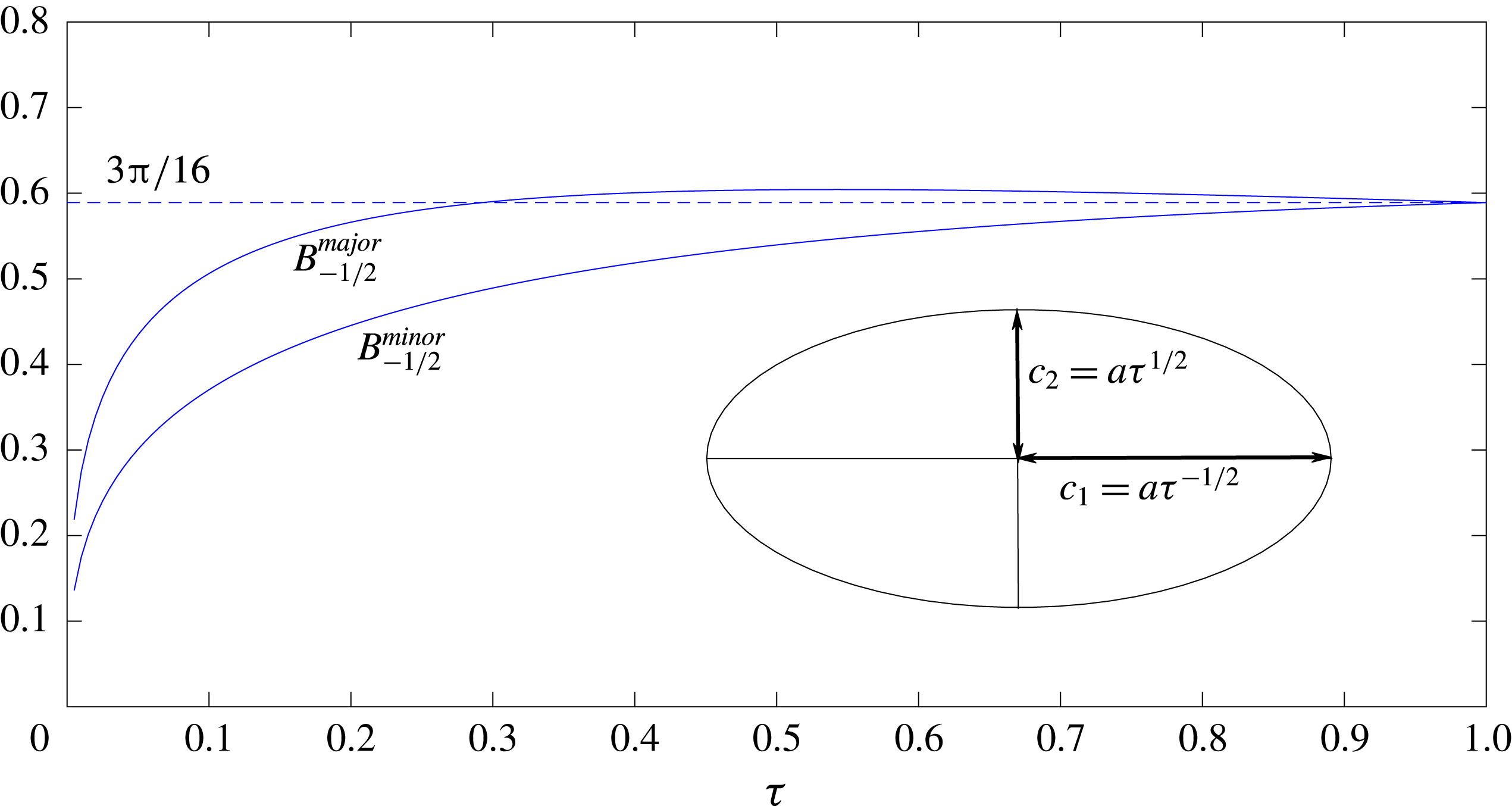
 $$\begin{eqnarray}B_{-1/2}^{\mathit{major}}=\frac{\unicode[STIX]{x1D70F}^{1/2}}{3{\mathcal{R}}(\unicode[STIX]{x1D70F})},\quad B_{-1/2}^{\mathit{minor}}=\frac{\unicode[STIX]{x1D70F}^{-1/2}}{3{\mathcal{R}}(1/\unicode[STIX]{x1D70F})}.\end{eqnarray}$$
The variation of these slip lengths with
 $\unicode[STIX]{x1D70F}$
is depicted in figure 2.
The degenerate case of a circular disk is recovered by considering the limit
 $\unicode[STIX]{x1D70F}\rightarrow 1$
. Thus, making use of the asymptotic approximations (Abramowitz & Stegun Reference Abramowitz and Stegun1965)
 $$\begin{eqnarray}K(m)\sim \frac{\unicode[STIX]{x03C0}}{2}+\frac{\unicode[STIX]{x03C0}m}{8}+\cdots \,,\quad E(m)\sim \frac{\unicode[STIX]{x03C0}}{2}-\frac{\unicode[STIX]{x03C0}m}{8}+\cdots \,,\end{eqnarray}$$
valid for
 $m\ll 1$
, we find that
 $\lim _{\unicode[STIX]{x1D70F}\rightarrow 1}{\mathcal{R}}(\unicode[STIX]{x1D70F})=16/9\unicode[STIX]{x03C0}$
. Both
 $O(\unicode[STIX]{x1D719}^{-1/2})$
slip lengths (A 2) then become
 $3\unicode[STIX]{x03C0}/16$
, in agreement with (5.7).
Principal
 $O(\unicode[STIX]{x1D719}^{-1/2})$
slip lengths for an ellipse of axis ratio
 $\unicode[STIX]{x1D70F}$
. The circular disk value
 $3\unicode[STIX]{x03C0}/16$
is indicated by the dashed line.

The other limit of a slender ellipse,
 $\unicode[STIX]{x1D70F}\rightarrow 0^{+}$
, is also of interest. Using the asymptotic behaviour of the elliptic integrals we find in that limit,
 $$\begin{eqnarray}{\mathcal{R}}(\unicode[STIX]{x1D70F})\sim \frac{4}{3}\left(2\ln \frac{4}{\unicode[STIX]{x1D70F}}-1\right)^{-1},\quad {\mathcal{R}}(1/\unicode[STIX]{x1D70F})\sim \frac{4}{3\unicode[STIX]{x1D70F}}\left(\ln \frac{4}{\unicode[STIX]{x1D70F}}+1\right)^{-1}.\end{eqnarray}$$
The diagonal components of
 $\unicode[STIX]{x1D64D}$
which correspond to the major and minor axes are accordingly given by
 $$\begin{eqnarray}\frac{8\unicode[STIX]{x03C0}}{\unicode[STIX]{x1D70F}^{1/2}}\left(2\ln \frac{4}{\unicode[STIX]{x1D70F}}-1\right)^{-1},\quad \frac{8\unicode[STIX]{x03C0}}{\unicode[STIX]{x1D70F}^{1/2}}\left(\ln \frac{4}{\unicode[STIX]{x1D70F}}+1\right)^{-1}.\end{eqnarray}$$
These agree with the slender-body approximations (8.7)–(8.8) obtained by Batchelor (Reference Batchelor1970) for the case of an ellipsoidal particle, when appropriately degenerated to the case of a flat elliptic disk. The corresponding
 $O(\unicode[STIX]{x1D719}^{-1/2})$
slip coefficients are
 $$\begin{eqnarray}B_{-1/2}^{\mathit{major}}\sim \frac{\unicode[STIX]{x1D70F}^{1/2}}{4}\left(2\ln \frac{4}{\unicode[STIX]{x1D70F}}-1\right),\quad B_{-1/2}^{\mathit{minor}}\sim \frac{\unicode[STIX]{x1D70F}^{1/2}}{4}\left(\ln \frac{4}{\unicode[STIX]{x1D70F}}+1\right).\end{eqnarray}$$
These may appear to imply an algebraic decrease with the aspect ratio
 $\unicode[STIX]{x1D70F}$
as the latter vanishes. Recalling, however, that the dimensionless slip-length tensor
 $\unicode[STIX]{x1D63D}_{-1/2}$
generically corresponds to normalisation by
 $\unicode[STIX]{x1D719}^{-1/2}l=\unicode[STIX]{x1D719}^{-1}a$
we find the dimensional slip lengths corresponding to (A 6),
 $$\begin{eqnarray}\frac{\unicode[STIX]{x1D719}^{-1}}{4}\left(2\ln \frac{4}{\unicode[STIX]{x1D70F}}-1\right)c_{2},\quad \frac{\unicode[STIX]{x1D719}^{-1}}{4}\left(\ln \frac{4}{\unicode[STIX]{x1D70F}}+1\right)c_{2}.\end{eqnarray}$$
For fixed
 $\unicode[STIX]{x1D719}$
and
 $c_{2}$
, these exhibit a logarithmic dependence upon
 $\unicode[STIX]{x1D70F}$
.
Appendix B. Lattice-sum asymptotics
Our goal is the asymptotic evaluation, as
 $x\rightarrow 0^{+}$
, of the lattice sum
 $$\begin{eqnarray}\mathop{\sum }_{\boldsymbol{k}\neq 0}\frac{k_{y}^{2}+k^{2}}{k^{3}}\text{e}^{-\text{i}\boldsymbol{k}\boldsymbol{\cdot }\hat{\boldsymbol{e}}_{x}x},\end{eqnarray}$$
appearing in (8.3). Making use of the auxiliary function
 ${\mathcal{F}}(k)$
we write this sum as
 $S_{1}+S_{2}$
, where
 $$\begin{eqnarray}S_{1}=\mathop{\sum }_{\boldsymbol{k}\neq \mathbf{0}}\frac{k_{y}^{2}+k^{2}}{k^{3}}\text{e}^{-\text{i}\boldsymbol{k}\boldsymbol{\cdot }\hat{\boldsymbol{e}}_{x}x}{\mathcal{F}}(k),\quad S_{2}=\mathop{\sum }_{\boldsymbol{k}\neq \mathbf{0}}\frac{k_{y}^{2}+k^{2}}{k^{3}}\text{e}^{-\text{i}\boldsymbol{k}\boldsymbol{\cdot }\hat{\boldsymbol{e}}_{x}x}[1-{\mathcal{F}}(k)],\end{eqnarray}$$
and apply the limit
 $x\rightarrow 0^{+}$
to each of these separately. Given the rapid large-
 $k$
decay of
 ${\mathcal{F}}(k)$
it is legitimate to set
 $x=0$
in
 $S_{1}$
, giving
 $$\begin{eqnarray}S_{1}\sim \mathop{\sum }_{\boldsymbol{k}\neq \mathbf{0}}\frac{k_{y}^{2}+k^{2}}{k^{3}}{\mathcal{F}}(k)+o(1)\quad \text{as}~x\rightarrow 0^{+}.\end{eqnarray}$$
The key to the asymptotic evaluation of
 $S_{2}$
is stipulation (8.6), which allows us to extend the summation to all
 $\boldsymbol{k}$
values:
 $$\begin{eqnarray}S_{2}=\mathop{\sum }_{\boldsymbol{k}}\frac{k_{y}^{2}+k^{2}}{k^{3}}\text{e}^{-\text{i}\boldsymbol{k}\boldsymbol{\cdot }\hat{\boldsymbol{e}}_{x}x}[1-{\mathcal{F}}(k)].\end{eqnarray}$$
By introducing a Dirac delta function at
 $\unicode[STIX]{x1D74E}=\boldsymbol{k}$
we write each term in the above sum as a double integral over the entire
 $\unicode[STIX]{x1D74E}$
-plane, namely
 $$\begin{eqnarray}\iint _{-\infty }^{\infty }\text{d}\unicode[STIX]{x1D714}_{x}\,\text{d}\unicode[STIX]{x1D714}_{y}\,\frac{\unicode[STIX]{x1D714}_{y}^{2}+\unicode[STIX]{x1D714}^{2}}{\unicode[STIX]{x1D714}^{3}}\text{e}^{-\text{i}\unicode[STIX]{x1D74E}\boldsymbol{\cdot }\hat{\boldsymbol{e}}_{x}x}[1-{\mathcal{F}}(\unicode[STIX]{x1D714})]\unicode[STIX]{x1D6FF}(\unicode[STIX]{x1D74E}-\boldsymbol{k}),\end{eqnarray}$$
wherein
 $\unicode[STIX]{x1D714}=|\unicode[STIX]{x1D74E}|$
. Formally interchanging summation and integration then gives
 $$\begin{eqnarray}S_{2}=\iint _{-\infty }^{\infty }\text{d}\unicode[STIX]{x1D714}_{x}\,\text{d}\unicode[STIX]{x1D714}_{y}\,\frac{\unicode[STIX]{x1D714}_{y}^{2}+\unicode[STIX]{x1D714}^{2}}{\unicode[STIX]{x1D714}^{3}}\text{e}^{-\text{i}\unicode[STIX]{x1D74E}\boldsymbol{\cdot }\hat{\boldsymbol{e}}_{x}x}[1-{\mathcal{F}}(\unicode[STIX]{x1D714})]\mathop{\sum }_{\boldsymbol{k}}\unicode[STIX]{x1D6FF}(\unicode[STIX]{x1D74E}-\boldsymbol{k}).\end{eqnarray}$$
At this point we employ the lattice identity (Nijboer & De Wette Reference Nijboer and De Wette1957)
 $$\begin{eqnarray}\mathop{\sum }_{\boldsymbol{k}}\unicode[STIX]{x1D6FF}(\unicode[STIX]{x1D74E}-\boldsymbol{k})=\frac{A}{4\unicode[STIX]{x03C0}^{2}}\mathop{\sum }_{\boldsymbol{r}}\text{e}^{-\text{i}\unicode[STIX]{x1D74E}\boldsymbol{\cdot }\boldsymbol{r}},\end{eqnarray}$$
where
 $\boldsymbol{r}$
is of the form (2.1) and the summation extends over all lattice points. Recalling (2.2) and interchanging again yields
 $$\begin{eqnarray}S_{2}=\mathop{\sum }_{\boldsymbol{r}}I(\boldsymbol{r}+\hat{\boldsymbol{e}}_{x}x),\end{eqnarray}$$
where
 $$\begin{eqnarray}I(\boldsymbol{q})=\frac{1}{4\unicode[STIX]{x03C0}}\iint _{-\infty }^{\infty }\text{d}\unicode[STIX]{x1D714}_{x}\,\text{d}\unicode[STIX]{x1D714}_{y}\,\frac{\unicode[STIX]{x1D714}_{y}^{2}+\unicode[STIX]{x1D714}^{2}}{\unicode[STIX]{x1D714}^{3}}\text{e}^{-\text{i}\unicode[STIX]{x1D74E}\boldsymbol{\cdot }\boldsymbol{q}}[1-{\mathcal{F}}(\unicode[STIX]{x1D714})].\end{eqnarray}$$
Using the polar coordinates
 $(\unicode[STIX]{x1D714},\unicode[STIX]{x1D717})$
of
 $\unicode[STIX]{x1D74E}$
and
 $(q,\unicode[STIX]{x1D717}_{q})$
of
 $\boldsymbol{q}$
we obtain
 $$\begin{eqnarray}I(\boldsymbol{q})=\frac{1}{4\unicode[STIX]{x03C0}}\int _{0}^{\infty }\text{d}\unicode[STIX]{x1D714}\,[1-{\mathcal{F}}(\unicode[STIX]{x1D714})]\int _{0}^{2\unicode[STIX]{x03C0}}\text{d}\unicode[STIX]{x1D717}\,\left(1+\sin ^{2}\unicode[STIX]{x1D717}\right)\text{e}^{-\text{i}\unicode[STIX]{x1D714}q\cos (\unicode[STIX]{x1D717}-\unicode[STIX]{x1D717}_{q})}.\end{eqnarray}$$
Consider first the contribution to
 $S_{2}$
from the point
 $\boldsymbol{r}=\mathbf{0}$
, namely
 $I(\hat{\boldsymbol{e}}_{x}x)$
. With
 $\unicode[STIX]{x1D717}_{q}=0$
in (B 10) evaluation of the inner integral is immediate, giving
 $$\begin{eqnarray}I(\hat{\boldsymbol{e}}_{x}x)=\frac{1}{2}\int _{0}^{\infty }[1-{\mathcal{F}}(\unicode[STIX]{x1D714})]\left[J_{0}(\unicode[STIX]{x1D714}x)+\frac{J_{1}(\unicode[STIX]{x1D714}x)}{\unicode[STIX]{x1D714}x}\right]\,\text{d}\unicode[STIX]{x1D714}.\end{eqnarray}$$
Asymptotic expansion at small
 $x$
then gives
 $$\begin{eqnarray}I(\hat{\boldsymbol{e}}_{x}x)\sim \frac{1}{x}-\frac{3}{4}\int _{0}^{\infty }{\mathcal{F}}(\unicode[STIX]{x1D714})\,\text{d}\unicode[STIX]{x1D714}+o(1)\quad \text{as}~x\rightarrow 0^{+}.\end{eqnarray}$$
In the contributions from the remaining points
 $\boldsymbol{r}\neq \mathbf{0}$
the limit
 $x\rightarrow 0$
is a regular one, allowing us to substitute
 $x=0$
to get the leading-order approximation. (Since (B 12) already provides the singular term which is necessitated by (8.3), this was to be expected.) Employing the polar coordinates
 $(r,\unicode[STIX]{x1D703})$
of
 $\boldsymbol{r}$
we find
 $$\begin{eqnarray}\lim _{x\rightarrow 0^{+}}I(\boldsymbol{r}+\hat{\boldsymbol{e}}_{x}x)={\textstyle \frac{1}{4}}\left[3M_{0}(r)+M_{2}(r)\cos 2\unicode[STIX]{x1D703}\right],\end{eqnarray}$$
where
 $$\begin{eqnarray}M_{n}(r)=\int _{0}^{\infty }[1-{\mathcal{F}}(\unicode[STIX]{x1D714})]J_{n}(\unicode[STIX]{x1D714}r)\,\text{d}\unicode[STIX]{x1D714}.\end{eqnarray}$$
Substitution into (B 8) of (B 12)–(B 13) provides the requisite approximation of
 $S_{2}$
. Addition of (B 3) then furnishes (8.7)–(8.8).