A general fluid–sediment mixture model and constitutive theory validated in many flow regimes

Aaron S. Baumgarten; Ken Kamrin

doi:10.1017/jfm.2018.914

A general fluid–sediment mixture model and constitutive theory validated in many flow regimes

Published online by Cambridge University Press: 28 December 2018

Aaron S. Baumgarten and

Ken Kamrin

Show author details

Aaron S. Baumgarten: Affiliation:
Department of Aeronautics and Astronautics, Massachusetts Institute of Technology, Cambridge, MA 02139, USA
Ken Kamrin*: Affiliation:
Department of Mechanical Engineering, Massachusetts Institute of Technology, Cambridge, MA 02139, USA
*: †Email address for correspondence: kkamrin@mit.edu

Article contents

Abstract
Introduction
Theory and formulation
Analytical verification of model
Numerical implementation
Results
Conclusion
References

Rights & Permissions

Abstract

We present a thermodynamically consistent constitutive model for fluid-saturated sediments, spanning dense to dilute regimes, developed from the basic balance laws for two-phase mixtures. The model can represent various limiting cases, such as pure fluid and dry grains. It is formulated to capture a number of key behaviours such as: (i) viscous inertial rheology of submerged wet grains under steady shearing flows, (ii) the critical state behaviour of grains, which causes granular Reynolds dilation/contraction due to shear, (iii) the change in the effective viscosity of the fluid due to the presence of suspended grains and (iv) the Darcy-like drag interaction observed in both dense and dilute mixtures, which gives rise to complex fluid–grain interactions under dilation and flow. The full constitutive model is combined with the basic equations of motion for each mixture phase and implemented in the material point method (MPM) to accurately model the coupled dynamics of the mixed system. Qualitative results show the breadth of problems which this model can address. Quantitative results demonstrate the accuracy of this model as compared with analytical limits and experimental observations of fluid and grain behaviours in inhomogeneous geometries.

JFM classification

Granular media: Granular media Multiphase and Particle-laden Flows: Multiphase and Particle-laden Flows Complex Fluids: Suspensions

Information

Type: JFM Papers
Information: Journal of Fluid Mechanics , Volume 861 , 25 February 2019, pp. 721 - 764
DOI: https://doi.org/10.1017/jfm.2018.914 [Opens in a new window]
Copyright: © 2018 Cambridge University Press

1 Introduction

Mixtures of fluids and sediments play an important role in many industrial and geotechnical engineering problems, from transporting large volumes of industrial wastes to building earthen levees and dams. To solve these problems, engineers have traditionally relied on the myriad of empirical models developed in the last century. These empirical models are derived by coupling relevant experimental observations to an understanding of the underlying physics governing the behaviour of these mixtures. The model reported in Einstein (Reference Einstein1906) describes the increase in effective fluid viscosity due to dilute suspensions of grains. The Darcy-like drag law given in Carman (Reference Carman1937) describes the pressure drop in a fluid as it flows through a bed of densely packed grains. The work by Turian & Yuan (Reference Turian and Yuan1977) characterizes the flow of slurries in pipelines. Other models (such as in Pailha & Pouliquen (Reference Pailha and Pouliquen2009)) describe more complex problems (such as the initiation of submerged granular avalanches); however, each of these models can only provide a description of a specific regime of mixture and flows.

To address an engineering problem that involves complex interactions of fluids and sediments spanning many flow regimes requires a more general modelling approach. A natural first step is to model the underlying physics directly by solving the coupled fluid–grain interactions at the micro-scale (as in the coupled lattice Boltzmann and discrete element method, LBM-DEM, proposed in Cook, Noble & Williams (Reference Cook, Noble and Williams2004)). Many problems of interest, however, involve far too much material for a direct approach to be computationally viable. We therefore turn to a continuum modelling approach, where the small-scale structures and physics are homogenized into bulk properties and behaviours.

Recent work simulating fluid–sediment mixtures as continua (see Soga et al. Reference Soga, Alonso, Yerro, Kumar and Bandara2015) presents a versatile foundation, but the reported results are highly sensitive to the choice of sediment constitutive model (see Ceccato & Simonini Reference Ceccato and Simonini2016 and Fern & Soga Reference Fern and Soga2016); even when pore pressure is uniform, no existing dry granular plasticity model correctly predicts the granular part of the rheology of saturated media. In this work, we carefully formulate a new set of constitutive rules governing the fluid and sediment phases of the continuum mixture. Using these rules, we construct a model that recovers the correct limiting behaviours – i.e. dry and viscous granular inertial rheologies, change of effective fluid viscosity due to suspended grains, Stokes and Carman–Kozeny drags and Reynolds dilation – and smoothly transitions between flow regimes covering the range from dense slurry-like flow to dilute suspensions. We implement our model in the material point method (MPM) and validate this implementation against several dynamic experiments involving submerged glass beads. We also consider the application of our model to the problems of slope collapse and intrusion.

2 Theory and formulation

Here we lay out the theoretical framework for the two-phase mixture model. In the formulation of this theory, we use the standard notation of continuum mechanics from Gurtin, Fried & Anand (Reference Gurtin, Fried and Anand2010). In particular, the trace of the tensor $\unicode[STIX]{x1D63C}$ is given by $\text{tr}\,\unicode[STIX]{x1D63C}$ and the transpose by $\unicode[STIX]{x1D63C}^{\top }$ . Every tensor admits the unique decomposition into a deviatoric part $\unicode[STIX]{x1D63C}_{0}$ and isotropic part by $\unicode[STIX]{x1D63C}=\unicode[STIX]{x1D63C}_{0}+(1/3)\text{tr}\,(\unicode[STIX]{x1D63C})\mathbf{1}$ with $\mathbf{1}$ the identity tensor.

2.1 Mixture theory

To develop the model we start by considering a mixture of grains and fluid. We assume that the grains are rough (i.e. physical, frictional contact can occur between grains; see Zhao & Davis (Reference Zhao and Davis2002)), made of incompressible material with true density $\unicode[STIX]{x1D70C}_{s}$ (i.e. the density of a grain) and essentially spherical with mean diameter $d$ . Additionally, we assume that the grains are quasi-mono-disperse (no size segregation during flow) and that grains are large enough to neglect Brownian effects (i.e. $d\gtrsim 100~\unicode[STIX]{x03BC}\text{m}$ for common engineering slurries). We also assume that the grains are fully immersed in a barotropic viscous fluid having true density $\unicode[STIX]{x1D70C}_{f}$ and viscosity $\unicode[STIX]{x1D702}_{0}$ . We use the term ‘true’ to mean those properties of the material in the mixture before the mixture is homogenized. A representative volume of material, $\unicode[STIX]{x1D6FA}$ , can therefore be decomposed into a solid volume, $\unicode[STIX]{x1D6FA}_{s}$ , and a fluid volume, $\unicode[STIX]{x1D6FA}_{f}$ , such that $\unicode[STIX]{x1D6FA}=\unicode[STIX]{x1D6FA}_{s}\cup \unicode[STIX]{x1D6FA}_{f}$ .

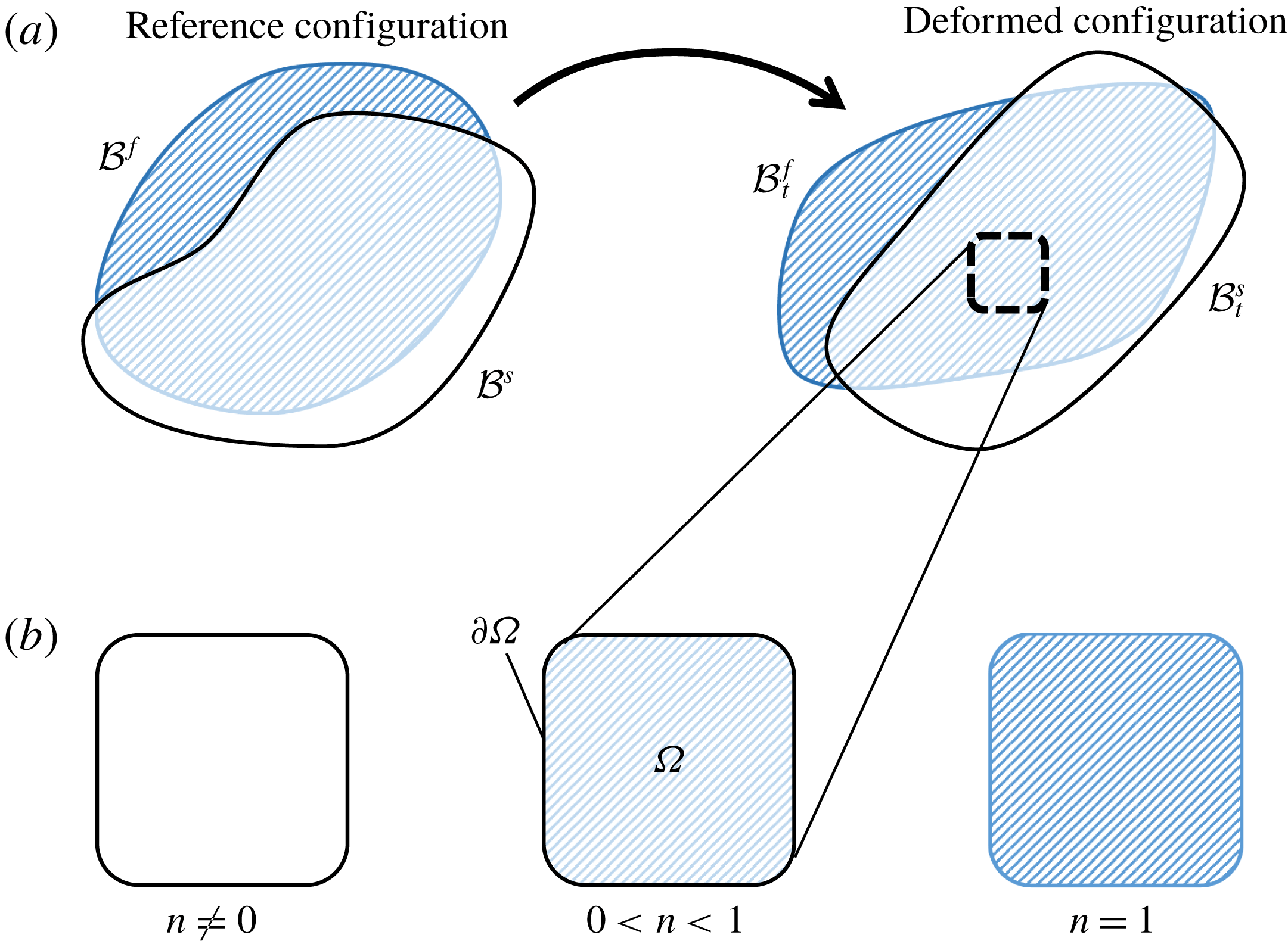
Figure 1 shows how this volume is decomposed and the important step of homogenizing the solid volume and fluid volume into two, overlapping continua. In the analysis that follows, $\unicode[STIX]{x1D713}_{s}$ will refer to some field $\unicode[STIX]{x1D713}$ defined on the solid phase, and $\unicode[STIX]{x1D713}_{f}$ will refer to some field $\unicode[STIX]{x1D713}$ defined on the fluid phase. If no subscript is given, then that field is defined on the mixture as a whole.

Figure 1.

Pictorial description of the representative volume $\unicode[STIX]{x1D6FA}$ , the decomposition of the domain into fluid and solid volumes, and the homogenization of the two phases.

2.1.1 Homogenization of phases

The effective densities, $\overline{\unicode[STIX]{x1D70C}}_{s}$ and $\overline{\unicode[STIX]{x1D70C}}_{f}$ , and phase velocities, $\boldsymbol{v}_{s}$ and $\boldsymbol{v}_{f}$ , of the mixture are defined such that conservation of mass and momentum in the continuum correspond to conservation of mass and momentum in the real mixture. For this, we consider a representative volume of material, $\unicode[STIX]{x1D6FA}$ , that contains a large number of individual grains. For the continuum approximation to be valid, large is defined such that grain-scale phenomena are smoothed out and bulk behaviour is captured. The volume of grains $\unicode[STIX]{x1D6FA}_{s}$ and volume of fluid $\unicode[STIX]{x1D6FA}_{f}$ within $\unicode[STIX]{x1D6FA}$ allow us to define the solid phase volume fraction or packing fraction, $\unicode[STIX]{x1D719}$ , and a fluid phase volume fraction or porosity, $n$ , as,

(2.1a,b )

$$\begin{eqnarray}\overline{\unicode[STIX]{x1D70C}}_{s}=\unicode[STIX]{x1D719}\unicode[STIX]{x1D70C}_{s},\quad \overline{\unicode[STIX]{x1D70C}}_{f}=n\unicode[STIX]{x1D70C}_{f},\quad \text{with}~\unicode[STIX]{x1D719}=1-n.\end{eqnarray}$$

The external body force acting on each homogenized phase (per unit volume), $\boldsymbol{b}_{0s}$ and $\boldsymbol{b}_{0f}$ , is proportional to the local effective density,

(2.2a,b )

$$\begin{eqnarray}\boldsymbol{b}_{0s}=\overline{\unicode[STIX]{x1D70C}}_{s}\boldsymbol{g},\quad \boldsymbol{b}_{0f}=\overline{\unicode[STIX]{x1D70C}}_{f}\boldsymbol{g},\end{eqnarray}$$

where $\boldsymbol{g}$ is the gravitational acceleration vector.

We next define the mixture Cauchy stress, $\unicode[STIX]{x1D748}$ , according to Cauchy’s theorem such that the stress response of the mixture is expressed as the sum of the phase-wise effective Cauchy stresses, $\unicode[STIX]{x1D748}_{s}$ and $\unicode[STIX]{x1D748}_{f}$ , i.e.

(2.3)

$$\begin{eqnarray}\unicode[STIX]{x1D748}=\unicode[STIX]{x1D748}_{s}+\unicode[STIX]{x1D748}_{f}.\end{eqnarray}$$

2.1.2 Overlapping continuum bodies

When considering a mixture problem, we begin by defining each phase as its own continuum body, as shown in figure 2(a). ${\mathcal{B}}^{s}$ defines the initial solid phase body (or reference body) and ${\mathcal{B}}^{f}$ defines the fluid phase reference body. At some later time $t$ , these bodies are represented by ${\mathcal{B}}_{t}^{s}$ and ${\mathcal{B}}_{t}^{f}$ .

To determine the behaviour of a volume of mixture $\unicode[STIX]{x1D6FA}$ , as shown in figure 2(b), we let that volume define a part in each continuum body. The full mixture is defined by the sum of these parts. If the volume of mixture is composed of fluid only, the porosity $n$ is unity. We also enforce that, in the absence of a solid phase, the local solid phase stress is zero, $\unicode[STIX]{x1D748}_{s}=\mathbf{0}$ . In this limit, we expect the behaviour of the mixture to be identical to that of a barotropic viscous fluid on its own. If the volume of mixture is solid only, the porosity $n$ is not zero (it would only be zero in the limit of vanishing pore space between grains). In this limit, the behaviour of the mixture should be identical to that of a dry granular material. To ensure this, we enforce that the local fluid phase stress is zero, $\unicode[STIX]{x1D748}_{f}=\mathbf{0}$ , and that the true fluid density, $\unicode[STIX]{x1D70C}_{f}$ , vanishes.

Figure 2.

(a) Pictorial definition of the reference bodies, ${\mathcal{B}}^{s}$ and ${\mathcal{B}}^{f}$ , and deformed bodies, ${\mathcal{B}}_{t}^{s}$ and ${\mathcal{B}}_{t}^{f}$ . (b) Parts in the deformed body are always fully saturated with porosity $n>0$ . In the limit of a fluid-only volume, the porosity $n=1$ . In the limit of a solid-only volume, we do not let the porosity $n$ go to zero, instead we let the fluid viscosity, bulk modulus and true density go to zero which effectively removes the fluid by making it stress and density free.

2.1.3 Mass conservation

We now define the equations governing the evolution of the true fluid density (i.e. the density of the fluid that is between the grains), $\unicode[STIX]{x1D70C}_{f}$ , and the effective densities of both phases, $\overline{\unicode[STIX]{x1D70C}}_{s}$ and $\overline{\unicode[STIX]{x1D70C}}_{f}$ . Recalling that the solid grains are assumed to be incompressible, $\unicode[STIX]{x1D70C}_{s}$ is constant. However, $\overline{\unicode[STIX]{x1D70C}}_{s}$ changes when the solid phase compacts or dilates as the structure of the granular skeleton changes. Since we will often have fields which belong to one phase or another (e.g. $\unicode[STIX]{x1D70C}_{s}$ belongs to the solid phase), it is convenient to define the material derivatives on each phase as follows,

(2.4a,b )

$$\begin{eqnarray}\frac{\text{D}^{s}\unicode[STIX]{x1D713}}{\text{D}t}=\frac{\unicode[STIX]{x2202}\unicode[STIX]{x1D713}}{\unicode[STIX]{x2202}t}+\boldsymbol{v}_{s}\boldsymbol{\cdot }\text{grad}\,\unicode[STIX]{x1D713},\quad \frac{\text{D}^{f}\unicode[STIX]{x1D713}}{\text{D}t}=\frac{\unicode[STIX]{x2202}\unicode[STIX]{x1D713}}{\unicode[STIX]{x2202}t}+\boldsymbol{v}_{f}\boldsymbol{\cdot }\text{grad}\,\unicode[STIX]{x1D713}.\end{eqnarray}$$

Mass conservation in a part of the solid phase continuum (as defined by a volume $\unicode[STIX]{x1D6FA}$ ) is enforced by setting the material derivative of solid mass in the volume to zero. As shown in Bandara & Soga (Reference Bandara and Soga2015), this requires that,

(2.5)

$$\begin{eqnarray}\frac{\text{D}^{s}\overline{\unicode[STIX]{x1D70C}}_{s}}{\text{D}t}+\overline{\unicode[STIX]{x1D70C}}_{s}\text{div}\,\boldsymbol{v}_{s}=0.\end{eqnarray}$$

A simple expansion of this expression using the definition of porosity from (2.1) yields an expression for the rate of change of the local measure of porosity,

(2.6)

$$\begin{eqnarray}\frac{\unicode[STIX]{x2202}n}{\unicode[STIX]{x2202}t}=(1-n)\text{div}\,\boldsymbol{v}_{s}-\boldsymbol{v}_{s}\boldsymbol{\cdot }\text{grad}\,n.\end{eqnarray}$$

Mass conservation of a fluid part defined by the arbitrary volume $\unicode[STIX]{x1D6FA}$ is enforced by,

(2.7)

$$\begin{eqnarray}\frac{\text{D}^{f}\overline{\unicode[STIX]{x1D70C}}_{f}}{\text{D}t}+\overline{\unicode[STIX]{x1D70C}}_{f}\text{div}\,\boldsymbol{v}_{f}=0.\end{eqnarray}$$

Combining (2.7) with (2.1) and (2.6), we find the correct form of the evolution law for the true fluid density,

(2.8)

$$\begin{eqnarray}\frac{n}{\unicode[STIX]{x1D70C}_{f}}\frac{\text{D}^{f}\unicode[STIX]{x1D70C}_{f}}{\text{D}t}=-\text{div}\,((1-n)\boldsymbol{v}_{s}+n\boldsymbol{v}_{f}).\end{eqnarray}$$

2.1.4 Momentum balance

Conservation of linear momentum is enforced locally for the each continuum body (see figure 2) as follows,

(2.9)

$$\begin{eqnarray}\displaystyle \left.\begin{array}{@{}c@{}}\displaystyle \overline{\unicode[STIX]{x1D70C}}_{s}\frac{\text{D}^{s}\boldsymbol{v}_{s}}{\text{D}t}=\boldsymbol{b}_{0s}-\boldsymbol{f}_{b}-\boldsymbol{f}_{d}+\text{div}\,\unicode[STIX]{x1D748}_{s}\\ \displaystyle \overline{\unicode[STIX]{x1D70C}}_{f}\frac{\text{D}^{f}\boldsymbol{v}_{f}}{\text{D}t}=\boldsymbol{b}_{0f}+\boldsymbol{f}_{b}+\boldsymbol{f}_{d}+\text{div}\,\unicode[STIX]{x1D748}_{f},\end{array}\right\} & & \displaystyle\end{eqnarray}$$

where $\boldsymbol{f}_{b}$ and $\boldsymbol{f}_{d}$ are inter-phase body forces. $\boldsymbol{f}_{d}$ is the inter-phase drag or Darcy’s law force. $\boldsymbol{f}_{b}$ has the form of the buoyant force described in Drumheller (Reference Drumheller2000) for immiscible mixtures,

(2.10)

$$\begin{eqnarray}\boldsymbol{f}_{b}=p_{f}\text{grad}\,(n).\end{eqnarray}$$

We let the solid phase stress $\unicode[STIX]{x1D748}_{s}$ take the classic form,

(2.11)

$$\begin{eqnarray}\unicode[STIX]{x1D748}_{s}=\tilde{\unicode[STIX]{x1D748}}-(1-n)p_{f}\mathbf{1}.\end{eqnarray}$$

The effective granular stress $\tilde{\unicode[STIX]{x1D748}}$ is the portion of the solid phase stress resulting from granular contact forces and from microscopic viscous stresses on grains from the fluid medium; it excludes the pressurization of the grains due to the pressure of the pore fluid. When the solid phase is dense, this also describes the Terzaghi effective stress that governs plastic flow of the solid phase. The term $p_{f}$ is the true fluid phase pore pressure. Since the fluid is barotropic, this is determined by the true fluid density $\unicode[STIX]{x1D70C}_{f}$ .

The expression for the fluid phase stress $\unicode[STIX]{x1D748}_{f}$ is,

(2.12)

$$\begin{eqnarray}\unicode[STIX]{x1D748}_{f}=\unicode[STIX]{x1D749}_{f}-np_{f}\mathbf{1}.\end{eqnarray}$$

The fluid phase stress is decomposed into a deviatoric part, $\unicode[STIX]{x1D749}_{f}$ , (i.e. $\text{tr}\,(\unicode[STIX]{x1D749}_{f})=0$ ) and a isotropic part, $np_{f}\mathbf{1}$ . With the expressions for the stresses and the buoyant body force given in (2.11), (2.12) and (2.10), we recover the equations of motion from Jackson (Reference Jackson2000).

The solid phase equation of motion is given as,

(2.13)

$$\begin{eqnarray}\overline{\unicode[STIX]{x1D70C}}_{s}\frac{\text{D}^{s}\boldsymbol{v}_{s}}{\text{D}t}=\overline{\unicode[STIX]{x1D70C}}_{s}\boldsymbol{g}-\boldsymbol{f}_{d}+\text{div}\,(\tilde{\unicode[STIX]{x1D748}})-(1-n)\text{grad}\,(p_{f})\end{eqnarray}$$

and the fluid phase equation of motion is given as,

(2.14)

$$\begin{eqnarray}\overline{\unicode[STIX]{x1D70C}}_{f}\frac{\text{D}^{f}\boldsymbol{v}_{f}}{\text{D}t}=\overline{\unicode[STIX]{x1D70C}}_{f}\boldsymbol{g}+\boldsymbol{f}_{d}+\text{div}\,(\unicode[STIX]{x1D749}_{f})-n\text{grad}\,(p_{f}).\end{eqnarray}$$

The equations in (2.13) and (2.14) fully describe the motion and behaviour of the mixture; however, we still need to define the specific rules governing the viscous drag between the phases $\boldsymbol{f}_{d}$ , the elastic–plastic behaviour of the solid phase $\tilde{\unicode[STIX]{x1D748}}$ , the pore fluid pressure $p_{f}$ and the viscous shear response of the fluid phase $\unicode[STIX]{x1D749}_{f}$ . By carefully defining these four constitutive rules, we capture the rheologically correct behaviour for mixtures of fluid and grains.

2.1.5 First and second laws of thermodynamics

To formulate the rules for $\boldsymbol{f}_{d}$ , $\tilde{\unicode[STIX]{x1D748}}$ , $p_{f}$ and $\unicode[STIX]{x1D749}_{f}$ , we start by defining the thermodynamic laws governing our mixture. When considering a single phase of material, it is often useful to assume that internal energy $(\unicode[STIX]{x1D700})$ , entropy $(s)$ and absolute temperature $(\unicode[STIX]{x1D717})$ are basic properties of a material. That is, they do not need to be defined in terms of other more basic properties. For our mixture model, we assume that analogous continuum fields exist describing the energy, entropy and temperature of the two continuum phases; however the physical basis of these fields is poorly defined (see Wilmanski Reference Wilmanski2008 and Klika Reference Klika2014). We therefore rely on the intuition developed in Gurtin et al. (Reference Gurtin, Fried and Anand2010) to specialize the thermodynamic analysis from Drumheller (Reference Drumheller2000) to a mixture of grains (represented by an elastic–plastic porous solid) with a barotropic viscous fluid.

The full thermodynamic analysis is shown in appendix A, and a brief summary of the resulting constitutive rules is given in table 1. Through the analysis, we find that the fluid pore pressure $p_{f}$ must be defined by the fluid phase specific free energy function $\hat{\unicode[STIX]{x1D713}}_{f}(\unicode[STIX]{x1D70C}_{f})$ and that the fluid shear stress $\unicode[STIX]{x1D749}_{f}$ and inter-phase drag $\boldsymbol{f}_{d}$ must both be dissipative, that is they must ‘resist’ their driving motion (the symmetric part of the fluid phase velocity gradient $\unicode[STIX]{x1D63F}_{f}$ and the difference in phase velocities $(\boldsymbol{v}_{s}-\boldsymbol{v}_{f})$ respectively). We also show that the solid phase effective granular stress $\tilde{\unicode[STIX]{x1D748}}$ can be expressed as that of an elastic–plastic solid with behaviour defined by (A 22). For these kinds of materials, the stress is determined by the strain–energy function $\hat{\unicode[STIX]{x1D711}}_{s}$ , which depends on the elastic part of the deformation gradient $\unicode[STIX]{x1D641}^{e}$ as defined in (A 13), which in turn defines the elastic volume Jacobian $J^{e}$ and the right elastic Cauchy–Green tensor $\unicode[STIX]{x1D63E}^{e}$ . The elastic tensor $\unicode[STIX]{x1D641}^{e}$ is a history dependent material tensor that evolves through time according to a decomposition of the solid phase strain rate $\unicode[STIX]{x1D63F}_{s}$ into an elastic strain rate $\unicode[STIX]{x1D63F}^{e}$ and a plastic part $\tilde{\unicode[STIX]{x1D63F}^{\,p}}$ according to (B 7) and subject to the dissipative inequality in (A 23). We note that in most common granular materials the bulk elastic deformations are extremely small, especially compared to plastic deformation, however grains do have finite stiffness and proper accounting of granular elasticity is important for thermodynamic consistency of the constitutive relations.

Figure 3.

The three regimes over which the inter-phase drag $\boldsymbol{f}_{d}$ must be defined. The normalized average drag force $\langle F\rangle$ is taken from van der Hoef, Beetstra & Kuipers (Reference van der Hoef, Beetstra and Kuipers2005) to be the average force on a single grain for a given packing fraction $\unicode[STIX]{x1D719}$ at a given flow rate.

Table 1.

Summary of thermodynamic rules for constitutive laws derived in appendix A.

2.2 Inter-phase drag law

The flow of a viscous fluid around and between grains of sediment will result in an inter-phase drag that we represent with the drag force $\boldsymbol{f}_{d}$ . This drag force can be understood as a body force acting on one phase by the other and has units $\text{N}~\text{m}^{-3}$ . In this work we assume that this force depends only on the relative velocities of the two phases $(\boldsymbol{v}_{s}-\boldsymbol{v}_{f})$ , the porosity of the mixture $n$ , the grain diameter $d$ and the fluid viscosity $\unicode[STIX]{x1D702}_{0}$ . We neglect dependence on material orientation or rotation (e.g. a fabric tensor) and neglect the effects of tortuosity (see Coussy Reference Coussy2004) on the apparent inter-phase drag.

For small flow velocities, the drag interaction between the fluid and the solid grains in the dilute limit shown in figure 3(a) is given analytically by the Stokes–Einstein equation.

(2.15)

$$\begin{eqnarray}\langle F\rangle =3\unicode[STIX]{x03C0}\unicode[STIX]{x1D702}_{0}\,\text{d}u,\end{eqnarray}$$

where $u$ is the free-steam flow speed. ‘Small’ here is taken to mean $Re\rightarrow 0$ with,

(2.16)

$$\begin{eqnarray}Re\equiv \frac{n\unicode[STIX]{x1D70C}_{f}\,\text{d}\Vert \boldsymbol{v}_{s}-\boldsymbol{v}_{f}\Vert }{\unicode[STIX]{x1D702}_{0}}.\end{eqnarray}$$

The leading $n$ in (2.16) is taken from Dupuit (Reference Dupuit1863) and relates the free-stream velocity to the average pore velocity. Normalizing the inter-phase drag by the volume average of the Stokes–Einstein drag on a single grain suggests the following functional form of $\boldsymbol{f}_{d}$ ,

(2.17)

$$\begin{eqnarray}\boldsymbol{f}_{d}=\frac{18\unicode[STIX]{x1D719}(1-\unicode[STIX]{x1D719})\unicode[STIX]{x1D702}_{0}}{d^{2}}\hat{F}(\unicode[STIX]{x1D719},Re)(\boldsymbol{v}_{s}-\boldsymbol{v}_{f}),\end{eqnarray}$$

with $\hat{F}(\unicode[STIX]{x1D719},Re)$ a function of non-dimensional parameters only. The only thermodynamic requirement on $\boldsymbol{f}_{d}$ (see (A 24)) is satisfied if $\hat{F}(\unicode[STIX]{x1D719},Re)\geqslant 0$ for all values of $\unicode[STIX]{x1D719}$ and $Re$ .

Determining the expression for $\hat{F}(\unicode[STIX]{x1D719},Re)$ for the full range of potential packing fractions $(0\leqslant \unicode[STIX]{x1D719}\lesssim 0.65)$ has historically been an intractable challenge. Analytical methods cannot be used for high Reynolds number flows $(Re>1)$ and flows with non-negligible packing fractions $(\unicode[STIX]{x1D719}>0)$ (see Clift, Grace & Weber Reference Clift, Grace and Weber2005). Experimentally, any loose packing $(\unicode[STIX]{x1D719}\lesssim 0.58)$ without sustained granular contacts will quickly compact, making the collection of accurate measurements near impossible.

Recent work by van der Hoef et al. (Reference van der Hoef, Beetstra and Kuipers2005) and Beetstra, van der Hoef & Kuipers (Reference Beetstra, van der Hoef and Kuipers2007) make use of the lattice-Boltzmann method to simulate the flow of fluid around mono- and bi-disperse packings of spheres for $0.10<\unicode[STIX]{x1D719}<0.6$ and $Re<1000$ . These simulations give the following form of $\hat{F}$ at low Reynolds numbers $(Re\rightarrow 0)$ ,

(2.18)

$$\begin{eqnarray}\hat{F}(\unicode[STIX]{x1D719},0)=\frac{10\unicode[STIX]{x1D719}}{(1-\unicode[STIX]{x1D719})^{2}}+(1-\unicode[STIX]{x1D719})^{2}(1+1.5\sqrt{\unicode[STIX]{x1D719}}),\end{eqnarray}$$

with the following high Reynolds number correction,

(2.19)

$$\begin{eqnarray}\hat{F}(\unicode[STIX]{x1D719},Re)=\hat{F}(\unicode[STIX]{x1D719},0)+\frac{0.413Re}{24(1-\unicode[STIX]{x1D719})^{2}}\left(\frac{(1-\unicode[STIX]{x1D719})^{-1}+3\unicode[STIX]{x1D719}(1-\unicode[STIX]{x1D719})+8.4Re^{-0.343}}{1+10^{3\unicode[STIX]{x1D719}}Re^{-(1+4\unicode[STIX]{x1D719})/2}}\right).\end{eqnarray}$$

In the dilute, low Reynolds number limit, (2.18) and (2.19) recover the Stokes–Einstein inter-phase drag. In the dense, low Reynolds number limit, (2.18) and (2.19) recover the Carman–Kozeny inter-phase drag from Carman (Reference Carman1937) as used in Bandara & Soga (Reference Bandara and Soga2015),

(2.20a,b )

$$\begin{eqnarray}\lim _{\unicode[STIX]{x1D719}\rightarrow 0}\hat{F}(\unicode[STIX]{x1D719},0)=1,\quad \lim _{\unicode[STIX]{x1D719}\rightarrow 1}\hat{F}(\unicode[STIX]{x1D719},0)=\frac{10\unicode[STIX]{x1D719}}{(1-\unicode[STIX]{x1D719})^{2}}.\end{eqnarray}$$

2.3 Fluid phase pore pressure

The fluid phase pore pressure is governed by the constitutive relation given in (A 20). We let the fluid phase free energy function, $\hat{\unicode[STIX]{x1D713}}(\unicode[STIX]{x1D70C}_{f})$ , be given by,

(2.21a,b )

$$\begin{eqnarray}\hat{\unicode[STIX]{x1D713}}_{f}(\unicode[STIX]{x1D70C}_{f})=\unicode[STIX]{x1D705}\left(\frac{\ln (\unicode[STIX]{x1D70C}_{0f})-\ln (\unicode[STIX]{x1D70C}_{f})-1}{\unicode[STIX]{x1D70C}_{f}^{2}}\right),\quad \text{such that }p_{f}=\unicode[STIX]{x1D705}\ln \left(\frac{\unicode[STIX]{x1D70C}_{f}}{\unicode[STIX]{x1D70C}_{0f}}\right),\end{eqnarray}$$

where $\unicode[STIX]{x1D70C}_{0f}$ is the true fluid density for which $p_{f}=0$ and $\unicode[STIX]{x1D705}$ is the fluid bulk modulus with units of Pa.

2.4 Fluid phase shear stress

We assume that the functional form of $\unicode[STIX]{x1D749}_{f}$ is given by, $\unicode[STIX]{x1D749}_{f}=\hat{\unicode[STIX]{x1D749}}_{f}(\unicode[STIX]{x1D63F}_{f},\unicode[STIX]{x1D719})$ with $\hat{\unicode[STIX]{x1D749}}_{f}$ isotropic and linear in $\unicode[STIX]{x1D63F}_{f}$ , the symmetric part of the fluid strain-rate tensor (see (A 9a,b )). From Truesdell & Noll (Reference Truesdell and Noll1965), the representation theorem for isotropic linear tensor functions requires that

(2.22)

$$\begin{eqnarray}\hat{\unicode[STIX]{x1D749}}_{f}(\unicode[STIX]{x1D63F}_{f},\unicode[STIX]{x1D719})=2\unicode[STIX]{x1D707}(\unicode[STIX]{x1D719})\unicode[STIX]{x1D63F}_{f}+\unicode[STIX]{x1D706}(\unicode[STIX]{x1D719})\text{tr}\,(\unicode[STIX]{x1D63F}_{f})\mathbf{1}.\end{eqnarray}$$

We assume $\unicode[STIX]{x1D749}_{f}$ is deviatoric, which requires $\unicode[STIX]{x1D706}(\unicode[STIX]{x1D719})=-(2/3)\unicode[STIX]{x1D707}(\unicode[STIX]{x1D719})$ . And the thermodynamic restriction on $\unicode[STIX]{x1D749}_{f}$ in (A 21) yields $\unicode[STIX]{x1D707}(\unicode[STIX]{x1D719})\geqslant 0$ . We let the effective fluid phase viscosity, $\unicode[STIX]{x1D707}(\unicode[STIX]{x1D719})$ , be given by the linear relation from Einstein (Reference Einstein1906) such that,

(2.23)

$$\begin{eqnarray}\unicode[STIX]{x1D749}_{f}=2\unicode[STIX]{x1D702}_{0}\left(1+{\textstyle \frac{5}{2}}\unicode[STIX]{x1D719}\right)\unicode[STIX]{x1D63F}_{0f},\end{eqnarray}$$

with $\unicode[STIX]{x1D702}_{0}$ defined previously as the true fluid viscosity.

2.5 Solid phase stress evolution

The solid phase effective granular stress is a function of the accumulated elastic deformation in the solid phase, $\unicode[STIX]{x1D641}^{e}$ , as defined in (A 22) (see table 1). In appendix B, we show that for stiff elastic materials, (A 22) is satisfied if the effective granular stress is evolved according to the following approximation using the Jaumann objective rate of $\tilde{\unicode[STIX]{x1D748}}$ ,

(2.24)

$$\begin{eqnarray}\overset{\unicode[STIX]{x1D6E5}}{\tilde{\unicode[STIX]{x1D748}}}\equiv \frac{\text{D}^{s}\tilde{\unicode[STIX]{x1D748}}}{\text{D}t}-\unicode[STIX]{x1D652}_{s}\tilde{\unicode[STIX]{x1D748}}+\tilde{\unicode[STIX]{x1D748}}\unicode[STIX]{x1D652}_{s}\approx \mathscr{C}[\unicode[STIX]{x1D63F}^{e}],\end{eqnarray}$$

with $\mathscr{C}$ an elastic stiffness tensor defined in (B 4), $\unicode[STIX]{x1D652}_{s}$ the skew part of the solid phase velocity gradient and $\unicode[STIX]{x1D63F}^{e}=\unicode[STIX]{x1D63F}_{s}-\tilde{\unicode[STIX]{x1D63F}^{\,p}}$ (see (B 7)). The material derivative of the effective granular stress is therefore given by,

(2.25)

$$\begin{eqnarray}\frac{\text{D}^{s}\tilde{\unicode[STIX]{x1D748}}}{\text{D}t}=2G\unicode[STIX]{x1D63F}^{e_{0}}+K\text{tr}\,(\unicode[STIX]{x1D63F}^{e})\mathbf{1}+\unicode[STIX]{x1D652}_{s}\tilde{\unicode[STIX]{x1D748}}-\tilde{\unicode[STIX]{x1D748}}\unicode[STIX]{x1D652}_{s}.\end{eqnarray}$$

In this way, we evolve the effective granular stress according to how the solid phase is straining $(\unicode[STIX]{x1D63F}_{s})$ minus how much of that strain rate is plastic $(\tilde{\unicode[STIX]{x1D63F}^{\,p}})$ . Physically, when the solid phase is flowing, most of the strain is accumulated plastically; when the solid phase is static (or resisting flow), strain is accumulated elastically. In this sense, through careful selection of the plastic flow rule $\tilde{\unicode[STIX]{x1D63F}^{\,p}}$ , the model can represent both flowing and static (sub-yield) behaviours of the solid phase.

2.6 Solid phase plastic flow rules

We let $\tilde{\unicode[STIX]{x1D63F}^{\,p}}$ have the following form,

(2.26)

$$\begin{eqnarray}\tilde{\unicode[STIX]{x1D63F}^{\,p}}=\frac{\dot{\bar{\unicode[STIX]{x1D6FE}}}^{p}}{\sqrt{2}}\frac{\tilde{\unicode[STIX]{x1D748}}_{0}}{\Vert \tilde{\unicode[STIX]{x1D748}}_{0}\Vert }+\frac{1}{3}(\unicode[STIX]{x1D6FD}\dot{\bar{\unicode[STIX]{x1D6FE}}}^{p}+\dot{\unicode[STIX]{x1D709}}_{1}+\dot{\unicode[STIX]{x1D709}}_{2})\mathbf{1},\end{eqnarray}$$

where the ‘over-dot’ operator $\dot{\unicode[STIX]{x1D713}}$ is equivalent to the material derivative $\text{D}^{s}\unicode[STIX]{x1D713}/\text{D}t$ . The only thermodynamic constraint on this plastic flow relation is given by (B 8). It is a simple exercise to show that the following formulation obeys that inequality.

Figure 4.

(a) In shear, the granular phase will obey critical state behaviour. This phenomenon is called Reynolds’ dilation and is captured by the rate of plastic dilation, $\unicode[STIX]{x1D6FD}\dot{\bar{\unicode[STIX]{x1D6FE}}}^{p}$ . (b) In expansion, the granular phase will come apart freely. This phenomenon is stress free and is captured by the rate of plastic expansion, $\dot{\unicode[STIX]{x1D709}}_{1}$ . (c) In compaction, granular collisions will result in a macroscopic pressure. This phenomenon is governed by the rate of plastic compaction, $-\dot{\unicode[STIX]{x1D709}}_{2}$ .

The equivalent plastic shear strain rate $\dot{\bar{\unicode[STIX]{x1D6FE}}}^{p}$ , the rate of plastic expansion $\dot{\unicode[STIX]{x1D709}}_{1}$ (figure 4 b), the rate of plastic compaction $-\dot{\unicode[STIX]{x1D709}}_{2}$ (figure 4 c) and the rate of Reynolds dilation $\unicode[STIX]{x1D6FD}\dot{\bar{\unicode[STIX]{x1D6FE}}}^{p}$ (figure 4 a) are the scalar measures that give the solid phase plastic flow. These flow measures are uniquely determined by the solid phase strain rate $\unicode[STIX]{x1D63F}_{s}$ , the solid phase effective stress $\tilde{\unicode[STIX]{x1D748}}$ and the current state of the mixture.

The dilation angle, $\unicode[STIX]{x1D6FD}$ , governs the rate of Reynolds dilation during plastic shear (see Rudnicki & Rice Reference Rudnicki and Rice1975; Roux & Radjai Reference Roux, Radjai, Herrmann, Hovi and Luding1998 and Roux & Radjai Reference Roux, Radjai, Aref and Phillips2001) and allows the material to dilate when shearing over-compacted grains and contract when shearing under-compacted grains. We use the functional form of $\unicode[STIX]{x1D6FD}$ given in Pailha & Pouliquen (Reference Pailha and Pouliquen2009),

(2.27)

$$\begin{eqnarray}\unicode[STIX]{x1D6FD}=K_{3}(\unicode[STIX]{x1D719}-\unicode[STIX]{x1D719}_{eq}),\end{eqnarray}$$

where $K_{3}$ is a unit-less material parameter and $\unicode[STIX]{x1D719}_{eq}$ is the rate-dependent equilibrium packing fraction achieved in steady-state shearing, given by Amarsid et al. (Reference Amarsid, Delenne, Mutabaruka, Monerie, Perales and Radjai2017) as,

(2.28)

$$\begin{eqnarray}\unicode[STIX]{x1D719}_{eq}=\frac{\unicode[STIX]{x1D719}_{m}}{1+aI_{m}},\end{eqnarray}$$

with $a$ a material parameter, $I_{m}$ the mixed inertial number and $\unicode[STIX]{x1D719}_{m}$ a material parameter describing the maximum possible packing fraction for a granular material in steady-state shearing flow. The non-dimensional inertial numbers (including the inertial number, $I$ , and the viscous inertial number, $I_{v}$ ) are defined as,

(2.29a-c )

$$\begin{eqnarray}I=\dot{\bar{\unicode[STIX]{x1D6FE}}}^{p}d\sqrt{\frac{\unicode[STIX]{x1D70C}_{s}}{\tilde{p}}},\quad I_{v}=\frac{\unicode[STIX]{x1D702}_{0}\dot{\bar{\unicode[STIX]{x1D6FE}}}^{p}}{\tilde{p}},\quad I_{m}=\sqrt{I^{2}+2I_{v}},\end{eqnarray}$$

with $\tilde{p}$ the granular pressure described in Boyer, Gauzelli & Pouliquen (Reference Boyer, Gauzelli and Pouliquen2011). The specific form of the mixed inertial number, $I_{m}$ , was determined in Amarsid et al. (Reference Amarsid, Delenne, Mutabaruka, Monerie, Perales and Radjai2017) by analysing numerous two-dimensional shearing flows spanning the inertial and viscous regimes ( $0\lesssim I\lesssim 0.1$ and $0\lesssim I_{v}\lesssim 0.2$ ).

To determine $\dot{\bar{\unicode[STIX]{x1D6FE}}}^{p}$ , $\dot{\unicode[STIX]{x1D709}}_{1}$ and $\dot{\unicode[STIX]{x1D709}}_{2}$ it is convenient to express their functional dependences implicitly in terms of the yield conditions given below. First, we uniquely define the equivalent plastic shear rate $\dot{\bar{\unicode[STIX]{x1D6FE}}}^{p}$ by solving

(2.30)

$$\begin{eqnarray}\left.\begin{array}{@{}c@{}}f_{1}=\bar{\unicode[STIX]{x1D70F}}-\max ((\unicode[STIX]{x1D707}_{p}+\unicode[STIX]{x1D6FD})\tilde{p},0)\\ f_{1}\leqslant 0,\quad \dot{\bar{\unicode[STIX]{x1D6FE}}}^{p}\geqslant 0,\quad f_{1}\dot{\bar{\unicode[STIX]{x1D6FE}}}^{p}=0,\end{array}\right\}\end{eqnarray}$$

with,

(2.31a,b )

$$\begin{eqnarray}\bar{\unicode[STIX]{x1D70F}}=\frac{\Vert \tilde{\unicode[STIX]{x1D748}}_{0}\Vert }{\sqrt{2}},\quad \tilde{p}=-\frac{1}{3}\text{tr}\,(\tilde{\unicode[STIX]{x1D748}}).\end{eqnarray}$$

Solutions to this system have non-zero plastic shearing only when the yield condition, $f_{1}=0$ , is met, and vanishing plastic shear rate when below yield, $f_{1}<0$ . We let $\unicode[STIX]{x1D707}_{p}=\hat{\unicode[STIX]{x1D707}}_{p}(\unicode[STIX]{x1D719},I_{v},I_{m})$ , which is formulated to capture both the $\unicode[STIX]{x1D707}(I)$ dry granular rheology from Jop, Forterre & Pouliquen (Reference Jop, Forterre and Pouliquen2006) and the $\unicode[STIX]{x1D707}(I_{v})$ low Stokes mixture rheology from Boyer et al. (Reference Boyer, Gauzelli and Pouliquen2011), as will be shown in § 3. The functional form of $\hat{\unicode[STIX]{x1D707}}_{p}$ is defined as,

(2.32)

$$\begin{eqnarray}\hat{\unicode[STIX]{x1D707}}_{p}(\unicode[STIX]{x1D719},I_{v},I_{m})=\unicode[STIX]{x1D707}_{1}+\frac{\unicode[STIX]{x1D707}_{2}-\unicode[STIX]{x1D707}_{1}}{1+(b/I_{m})}+\frac{5}{2}\left(\frac{\unicode[STIX]{x1D719}I_{v}}{aI_{m}}\right).\end{eqnarray}$$

Note that in steady-state shearing, $\unicode[STIX]{x1D719}=\unicode[STIX]{x1D719}_{eq}$ and $\hat{\unicode[STIX]{x1D707}}_{p}$ reduces to a function of $I_{v}$ and $I_{m}$ only.

Granular separation, represented by the rate of plastic expansion, $\dot{\unicode[STIX]{x1D709}_{1}}$ , is obtained from the conditions

(2.33)

$$\begin{eqnarray}\left.\begin{array}{@{}c@{}}f_{2}=-\tilde{p}\\ f_{2}\leqslant 0,\quad \dot{\unicode[STIX]{x1D709}}_{1}\geqslant 0,\quad f_{2}\dot{\unicode[STIX]{x1D709}}_{1}=0.\end{array}\right\}\end{eqnarray}$$

These conditions enforce the assumption that non-cohesive grains cannot support tension. Hence, the granular media undergoes plastic expansion $\dot{\unicode[STIX]{x1D709}}_{1}$ , representing grain separation, in lieu of developing tensile granular stress states.

The flow rule governing plastic compaction, $-\dot{\unicode[STIX]{x1D709}}_{2}$ , arises from solving the system below:

(2.34)

$$\begin{eqnarray}\left.\begin{array}{@{}c@{}}f_{3}=g(\unicode[STIX]{x1D719})\tilde{p}-(a\unicode[STIX]{x1D719})^{2}[(\dot{\bar{\unicode[STIX]{x1D6FE}}}^{p}-K_{4}\dot{\unicode[STIX]{x1D709}}_{2})^{2}d^{2}\unicode[STIX]{x1D70C}_{s}+2\unicode[STIX]{x1D702}_{0}(\dot{\bar{\unicode[STIX]{x1D6FE}}}^{p}-K_{4}\dot{\unicode[STIX]{x1D709}}_{2})]\\ f_{3}\leqslant 0,\quad \dot{\unicode[STIX]{x1D709}}_{2}\leqslant 0,\quad f_{3}\dot{\unicode[STIX]{x1D709}}_{2}=0,\end{array}\right\}\end{eqnarray}$$

with,

(2.35)

$$\begin{eqnarray}g(\unicode[STIX]{x1D719})=\left\{\begin{array}{@{}ll@{}}(\unicode[STIX]{x1D719}_{m}-\unicode[STIX]{x1D719})^{2}\quad & \text{if }\unicode[STIX]{x1D719}<\unicode[STIX]{x1D719}_{m}\\ 0\quad & \text{if }\unicode[STIX]{x1D719}\geqslant \unicode[STIX]{x1D719}_{m}.\end{array}\right.\end{eqnarray}$$

The form of $g(\unicode[STIX]{x1D719})$ and the $f_{3}$ yield surface are chosen such that, when the material is being compacted or sheared but is less dense than the critical packing, $\unicode[STIX]{x1D719}<\unicode[STIX]{x1D719}_{m}$ , there is an upper bound on the admissible effective pressure $\tilde{p}$ . However, in the compacted regime, $\unicode[STIX]{x1D719}\geqslant \unicode[STIX]{x1D719}_{m}$ , any pressure is admissible, as the grains are assumed to always be touching. The upper bound on the value of $\tilde{p}$ is determined by inverting the expression for $\unicode[STIX]{x1D719}_{eq}$ defined in (2.28). The unit-less $K_{4}$ coefficient defines the relative importance of the plastic compaction rate in determining this upper bound compared to the plastic shear rate.

Together (2.25), (2.26), (B 7), (2.30), (2.33) and (2.34) uniquely determine the plastic flow rates $\dot{\bar{\unicode[STIX]{x1D6FE}}}^{p}$ , $\dot{\unicode[STIX]{x1D709}}_{1}$ and $\dot{\unicode[STIX]{x1D709}}_{2}$ . It is also important to note that the specific forms of (2.33) and (2.34) restrict $\dot{\unicode[STIX]{x1D709}}_{1}$ to be zero when plastic compaction occurs and restrict $\dot{\unicode[STIX]{x1D709}}_{2}$ to be zero when plastic expansion occurs.

2.7 Summary of model assumptions

The model presented in this section is formulated to capture several key phenomena observed in mixtures of fluids and grains. In the development of this model we have assumed that the granular material is quasi-mono-disperse, composed of incompressible cohesion-less solid grains, and fully saturated with an isothermal Newtonian liquid. We have neglected Brownian effects on the mixture, limiting the applicability of our model to the study of granular mixtures which are dominated by gravitational energy or by shearing time scales ( $d\gtrsim 100~\unicode[STIX]{x03BC}\text{m}$ for common engineering slurries). In addition, the evolution law for the effective granular stress (including the plastic flow rule) is only applicable in the limit of stiff elasticity ( $G,~K\gg \tilde{p}$ ).

We have derived our inter-phase drag law (see (2.17)) from the empirical relations given in Carman (Reference Carman1937), van der Hoef et al. (Reference van der Hoef, Beetstra and Kuipers2005) and Beetstra et al. (Reference Beetstra, van der Hoef and Kuipers2007). The simulations and experiments that underpin these empirical relations suggest that this drag law is applicable for $0\leqslant \unicode[STIX]{x1D719}\lesssim 0.65$ and $Re\leqslant 1000$ . In addition the internal friction coefficient for the solid phase (see (2.32)) is developed through consideration of models presented in Stickel & Powell (Reference Stickel and Powell2005), Boyer et al. (Reference Boyer, Gauzelli and Pouliquen2011) and Amarsid et al. (Reference Amarsid, Delenne, Mutabaruka, Monerie, Perales and Radjai2017). The data which underpin these empirical models suggest that the internal friction model is applicable for $I\lesssim 0.2,$ $I_{v}\lesssim 0.1$ , $I_{m}\lesssim 0.6$ and $0\leqslant St<\infty$ .

3 Analytical verification of model

In this section we verify that the model laid out in § 2 has the correct limiting behaviour in a simple shearing flow. In particular we are interested in showing that under the appropriate conditions, the following rheologies are captured.

(i) $\unicode[STIX]{x1D707}(I)$ , $\unicode[STIX]{x1D719}(I)$ steady-state dry granular inertial rheology.
(ii) $\unicode[STIX]{x1D707}(I_{v})$ , $\unicode[STIX]{x1D719}(I_{v})$ steady-state viscous inertial rheology.
(iii) $\unicode[STIX]{x1D702}_{r}(\unicode[STIX]{x1D719})$ slurry/suspension effective viscosity.

These phenomena should arise as different cases of steady shearing flow wherein the mixture is co-moving such that, $\boldsymbol{v}_{s}=\boldsymbol{v}_{f}$ and,

(3.1)

$$\begin{eqnarray}\text{grad}\,(\boldsymbol{v}_{s})=\text{grad}\,(\boldsymbol{v}_{f})=\unicode[STIX]{x1D647}=\left[\begin{array}{@{}ccc@{}}0 & \dot{\unicode[STIX]{x1D6FE}} & 0\\ 0 & 0 & 0\\ 0 & 0 & 0\end{array}\right],\end{eqnarray}$$

where $\dot{\unicode[STIX]{x1D6FE}}$ is the applied steady shear rate. Since the mixture is uniform and $\text{tr}\,(\unicode[STIX]{x1D647})=0$ , (2.8) tells us that the true fluid density, $\unicode[STIX]{x1D70C}_{f}$ , is constant. By (2.21), this means that the fluid phase pore pressure remains constant, $p_{f}=p_{eq}$ , with $p_{eq}$ some constant equilibrium pressure.

The fluid phase shear stress, $\unicode[STIX]{x1D749}_{f}$ , is determined by (2.23),

(3.2)

$$\begin{eqnarray}\unicode[STIX]{x1D749}_{f}=\unicode[STIX]{x1D702}_{0}\left(1+\frac{5}{2}\unicode[STIX]{x1D719}\right)\left[\begin{array}{@{}ccc@{}}0 & \dot{\unicode[STIX]{x1D6FE}} & 0\\ \dot{\unicode[STIX]{x1D6FE}} & 0 & 0\\ 0 & 0 & 0\end{array}\right].\end{eqnarray}$$

In the solid phase, there are two regimes of interest, the compacted regime with $\unicode[STIX]{x1D719}\geqslant \unicode[STIX]{x1D719}_{m}$ and the non-compacted regime with $\unicode[STIX]{x1D719}<\unicode[STIX]{x1D719}_{m}$ . In the compacted regime, the sustained granular contacts result in non-steady behaviour (the positivity of the dilatation angle $\unicode[STIX]{x1D6FD}$ from (2.27) results in continuous growth of the pressure $\tilde{p}$ ). For this reason, we will be more interested in the behaviour of the non-compacted regime, where steady-state flow is possible.

Assuming that the solid phase begins in a stress-free state and that the shear modulus, $G$ , is much greater than the characteristic shear stress, it can be shown that (2.25) and (2.26) together imply that $\tilde{\unicode[STIX]{x1D748}}$ will reach a steady value with the equivalent plastic shear rate $\dot{\bar{\unicode[STIX]{x1D6FE}}}^{p}$ non-zero and equivalent to the total steady shear rate $\dot{\unicode[STIX]{x1D6FE}}$ . The solid phase effective granular stress then satisfies,

(3.3)

$$\begin{eqnarray}\tilde{\unicode[STIX]{x1D748}}\approx \left[\begin{array}{@{}ccc@{}}\tilde{p} & \unicode[STIX]{x1D707}_{p}\tilde{p} & 0\\ \unicode[STIX]{x1D707}_{p}\tilde{p} & \tilde{p} & 0\\ 0 & 0 & \tilde{p}\end{array}\right].\end{eqnarray}$$

The total mixture stress as defined in (2.3) is characterized by the mixture pressure $p=-(1/3)\text{tr}\,(\unicode[STIX]{x1D748})$ and the mixture shear stress $\unicode[STIX]{x1D70F}=(1/\sqrt{2})\Vert \unicode[STIX]{x1D748}_{0}\Vert$ . In the case of steady shearing flow we find,

(3.4)

$$\begin{eqnarray}\left.\begin{array}{@{}c@{}}\unicode[STIX]{x1D70F}=\unicode[STIX]{x1D702}_{0}(1+{\textstyle \frac{5}{2}}\unicode[STIX]{x1D719})\dot{\unicode[STIX]{x1D6FE}}+\unicode[STIX]{x1D707}_{p}\tilde{p}\\ p=p_{eq}+\tilde{p},\end{array}\right\}\end{eqnarray}$$

with the steady-state packing fraction, $\unicode[STIX]{x1D719}=\unicode[STIX]{x1D719}_{eq}$ , given by (2.28).

3.1 Dry granular flow

In steady simple shear flow, dry granular materials have been shown to obey the $\unicode[STIX]{x1D707}(I)$ and $\unicode[STIX]{x1D719}(I)$ rheology as given in Jop et al. (Reference Jop, Forterre and Pouliquen2006) and Da Cruz et al. (Reference Da Cruz, Emam, Prochnow, Roux and Chevoir2005),

(3.5a,b )

$$\begin{eqnarray}\unicode[STIX]{x1D707}(I)=\unicode[STIX]{x1D707}_{1}+\frac{\unicode[STIX]{x1D707}_{2}-\unicode[STIX]{x1D707}_{1}}{1+(I_{0}/I)},\quad \text{and}\quad \unicode[STIX]{x1D719}(I)=\unicode[STIX]{x1D719}_{m}-cI,\end{eqnarray}$$

with $c$ some material constant and where $\unicode[STIX]{x1D707}(I)$ is the ratio between the measured shear stress $\unicode[STIX]{x1D70F}$ and the measured granular pressure $\tilde{p}$ . This behaviour is captured by our model in the limit that $\unicode[STIX]{x1D702}_{0}\rightarrow 0$ . By the definitions of the inertial numbers in (2.29), if $\unicode[STIX]{x1D702}_{0}=0$ , then $I_{m}=I$ . Additionally, for $\unicode[STIX]{x1D702}_{0}=0$ , $\unicode[STIX]{x1D707}=\unicode[STIX]{x1D707}_{p}$ , as given in (2.32). Expanding the expression for $\unicode[STIX]{x1D719}_{eq}$ from (2.28) around $I=0$ (where existing data have been collected), we find that our model predicts the following steady shear behaviour,

(3.6a,b )

$$\begin{eqnarray}\unicode[STIX]{x1D707}=\unicode[STIX]{x1D707}_{1}+\frac{\unicode[STIX]{x1D707}_{2}-\unicode[STIX]{x1D707}_{1}}{1+(b/I)},\quad \text{and}\quad \unicode[STIX]{x1D719}\approx \unicode[STIX]{x1D719}_{m}-a\unicode[STIX]{x1D719}_{m}I+O(I^{2}),\end{eqnarray}$$

which is a reasonable approximation to known fits of the $\unicode[STIX]{x1D707}(I)$ , $\unicode[STIX]{x1D719}(I)$ rheology if $a=(c/\unicode[STIX]{x1D719}_{m})$ and $b=I_{0}$ .

3.2 Viscous granular mixtures

Boyer et al. (Reference Boyer, Gauzelli and Pouliquen2011) experimentally investigate the steady-state rheology of mixtures undergoing steady, quasi-two-dimensional shear flow at low Stokes numbers. The Stokes number of interest in this context is defined in Amarsid et al. (Reference Amarsid, Delenne, Mutabaruka, Monerie, Perales and Radjai2017) as,

(3.7)

$$\begin{eqnarray}St=\frac{\unicode[STIX]{x1D70C}_{s}d^{2}\dot{\unicode[STIX]{x1D6FE}}}{\unicode[STIX]{x1D702}_{0}}=\frac{I^{2}}{I_{v}}.\end{eqnarray}$$

In the limit that $St\rightarrow 0$ , the mixed inertial number $I_{m}$ is dominated by the viscous inertial number $I_{v}$ , such that $I_{m}=\sqrt{2I_{v}}$ .

Boyer et al. (Reference Boyer, Gauzelli and Pouliquen2011) defines the $\unicode[STIX]{x1D707}(I_{v})$ and $\unicode[STIX]{x1D719}(I_{v})$ viscous granular rheologies as follows,

(3.8a,b )

$$\begin{eqnarray}\unicode[STIX]{x1D707}(I_{v})=\unicode[STIX]{x1D707}_{1}+\frac{\unicode[STIX]{x1D707}_{2}-\unicode[STIX]{x1D707}_{1}}{1+(I_{0}/I_{v})}+I_{v}+\frac{5}{2}\unicode[STIX]{x1D719}_{m}\sqrt{I_{v}}\quad \text{and}\quad \unicode[STIX]{x1D719}(I_{v})=\frac{\unicode[STIX]{x1D719}_{m}}{1+\sqrt{I_{v}}}.\end{eqnarray}$$

It can be shown from (2.28), (2.29) and (2.32) that the steady shear response of our mixture is given by,

(3.9a,b )

$$\begin{eqnarray}\unicode[STIX]{x1D707}(I_{v},I_{m})=\unicode[STIX]{x1D707}_{1}+\frac{\unicode[STIX]{x1D707}_{2}-\unicode[STIX]{x1D707}_{1}}{1+(b/\sqrt{2I_{v}})}+I_{v}+\frac{5}{2}\unicode[STIX]{x1D719}_{m}\sqrt{\frac{I_{v}}{2a^{2}}},\quad \text{and}\quad \unicode[STIX]{x1D719}=\frac{\unicode[STIX]{x1D719}_{m}}{1+a\sqrt{2I_{v}}}.\end{eqnarray}$$

The expression for the steady-state packing fraction $\unicode[STIX]{x1D719}$ in (3.9) identically recovers the $\unicode[STIX]{x1D719}(I_{v})$ fit from Boyer et al. (Reference Boyer, Gauzelli and Pouliquen2011) when $a=(1/\sqrt{2})$ . The $\unicode[STIX]{x1D707}(I_{v})$ function of Boyer et al. 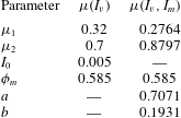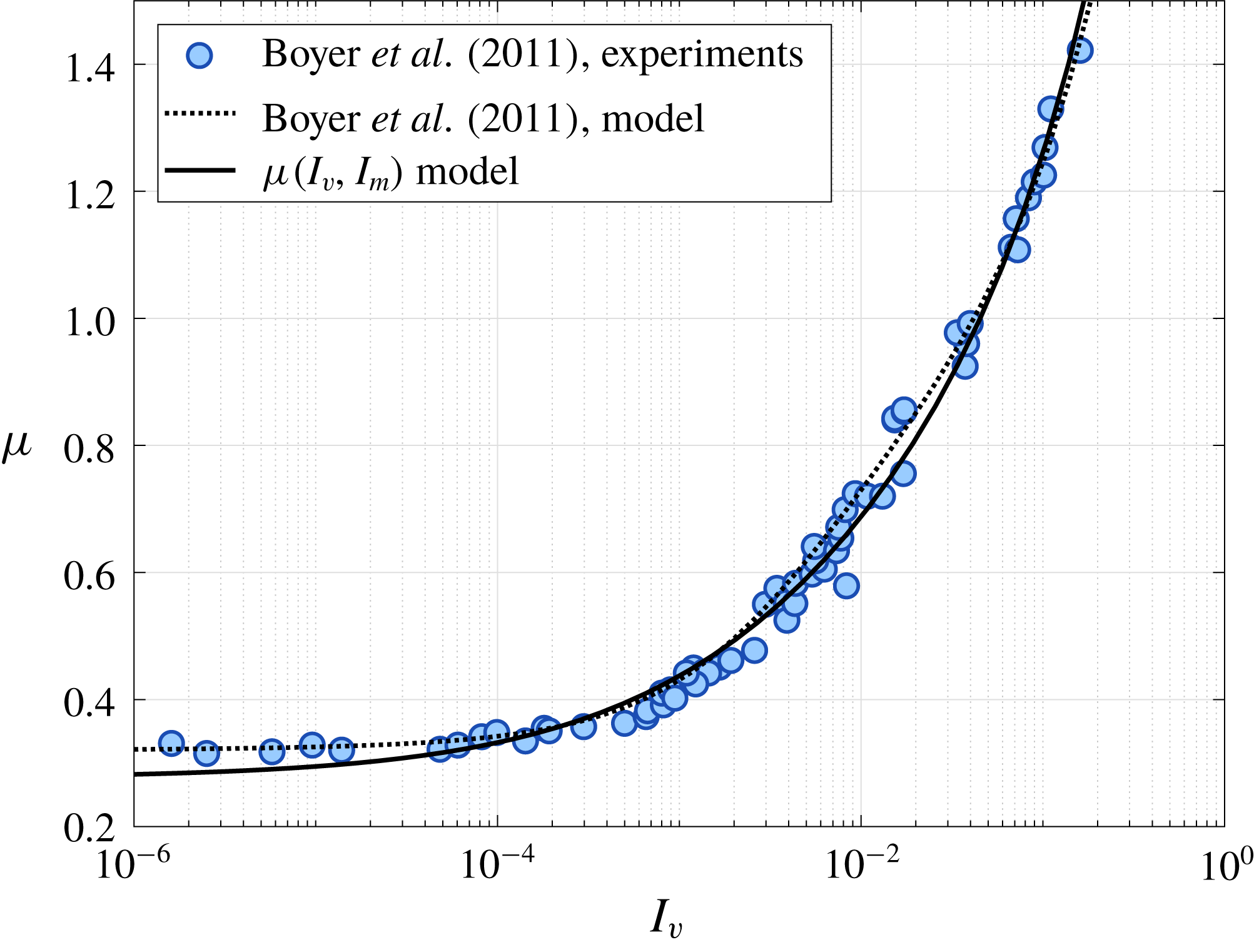(Reference Boyer, Gauzelli and Pouliquen2011) is not reproduced exactly with our model; however, as shown in figure 5, we can fit our form $\unicode[STIX]{x1D707}(I_{v},I_{m})$ to their data directly. Strong agreement is found between our model fit, the model fit in Boyer et al. (Reference Boyer, Gauzelli and Pouliquen2011) and the data collected in that work. The fit parameters for the plot in figure 5 are given in table 2.

Table 2.

Parameters for model fit to data in figure 5.

Figure 5.

Plot of the ratio between the shear stress and effective granular pressure ( $\unicode[STIX]{x1D707}$ ) against the inertial number $I_{v}$ . Data collected by Boyer et al. (Reference Boyer, Gauzelli and Pouliquen2011) are shown as the shaded blue circles. The $\unicode[STIX]{x1D707}(I_{v})$ rheology from that work is represented by the dotted line. The combined response of the mixture model presented in this work (see (3.9)) is represented by the solid line.

3.3 Suspension effective viscosity

Significant work has been done on understanding the behaviour of co-moving suspensions of granular material in fluids. We are particularly interested in the change in effective fluid viscosity of suspensions due to the solid phase volume fraction as reviewed and summarized in Stickel & Powell (Reference Stickel and Powell2005) with $\unicode[STIX]{x1D702}_{r}$ , the relative viscosity,

(3.10a-c )

$$\begin{eqnarray}\unicode[STIX]{x1D702}_{r}=\frac{\unicode[STIX]{x1D70F}}{\unicode[STIX]{x1D702}_{0}\dot{\unicode[STIX]{x1D6FE}}},\quad \lim _{\unicode[STIX]{x1D719}\rightarrow \unicode[STIX]{x1D719}_{m}}\unicode[STIX]{x1D702}_{r}=\infty ,\quad \lim _{\unicode[STIX]{x1D719}\rightarrow 0}\frac{\unicode[STIX]{x1D702}_{r}-1}{\unicode[STIX]{x1D719}}=[\unicode[STIX]{x1D702}].\end{eqnarray}$$

In the dense limit ( $\unicode[STIX]{x1D719}\rightarrow \unicode[STIX]{x1D719}_{m}$ ), the viscosity of the suspension approaches infinity and in the dilute limit ( $\unicode[STIX]{x1D719}\rightarrow 0$ ), the viscosity of the mixture should vary linearly with $[\unicode[STIX]{x1D702}]$ where $[\unicode[STIX]{x1D702}]=(5/2)$ for hard spheres (Stickel & Powell Reference Stickel and Powell2005).

As in § 3.2, we are concerned with the behaviour of our mixture model in the low Stokes limit such that $I_{m}=\sqrt{2I_{v}}$ . Therefore we find, $\unicode[STIX]{x1D702}_{r}=1+(5/2)\unicode[STIX]{x1D719}+(\unicode[STIX]{x1D707}_{p}/I_{v})$ , which by (2.28) and (2.32) is equivalently,

(3.11)

$$\begin{eqnarray}\unicode[STIX]{x1D702}_{r}(\unicode[STIX]{x1D719})=1+\frac{5}{2}\unicode[STIX]{x1D719}\left(\frac{\unicode[STIX]{x1D719}_{m}}{\unicode[STIX]{x1D719}_{m}-\unicode[STIX]{x1D719}}\right)+2\left(\frac{a\unicode[STIX]{x1D719}}{\unicode[STIX]{x1D719}_{m}-\unicode[STIX]{x1D719}}\right)^{2}\left(\unicode[STIX]{x1D707}_{1}+\frac{\unicode[STIX]{x1D707}_{2}-\unicode[STIX]{x1D707}_{1}}{1+ab\unicode[STIX]{x1D719}/(\unicode[STIX]{x1D719}_{m}-\unicode[STIX]{x1D719})}\right).\end{eqnarray}$$

It can be shown that this relation achieves both limiting behaviours required of effective viscosity models.

By noting the similarity of the materials used by Chang & Powell (Reference Chang and Powell1994) (polystyrene and poly(methyl methacrylate)), to that used in Boyer et al. (Reference Boyer, Gauzelli and Pouliquen2011), we use the coefficients determined in § 3.2 and given in table 2 to compare (3.11) against the experimental measurements reported in Chang & Powell (Reference Chang and Powell1994) and Boyer et al. (Reference Boyer, Gauzelli and Pouliquen2011) (see figure 6).

Figure 6.

Plot of various models for effective viscosity $\unicode[STIX]{x1D702}_{r}$ versus the relative packing fraction $\unicode[STIX]{x1D719}/\unicode[STIX]{x1D719}_{m}$ . The model given in this work by (3.11) is shown by the solid line. The red diamonds represent the experimental results reported in Chang & Powell (Reference Chang and Powell1994) (from Chong, Christiansen & Baer (Reference Chong, Christiansen and Baer1971), Poslinski et al. (Reference Poslinski, Ryan, Gupta, Seshadri and Frechette1988), Storms, Ramarao & Weiland (Reference Storms, Ramarao and Weiland1990), Shapiro & Probstein (Reference Shapiro and Probstein1992), Chang & Powell (Reference Chang and Powell1993) and Chang & Powell (Reference Chang and Powell1994)). The blue circles represent the experimental results reported in Boyer et al. (Reference Boyer, Gauzelli and Pouliquen2011).

4 Numerical implementation

We are interested in time-accurate simulations of fluid–sediment mixtures undergoing arbitrarily large deformations. To do this, we use a material point method (MPM) framework capable of simultaneously solving all of the governing equations shown in table 3. This MPM framework is a derivative of that shown in Dunatunga & Kamrin (Reference Dunatunga and Kamrin2015) and borrows heavily from methods described in Abe, Soga & Bandara (Reference Abe, Soga and Bandara2013) and Bandara & Soga (Reference Bandara and Soga2015).

Table 3.

Summary of governing equations derived in § 2.

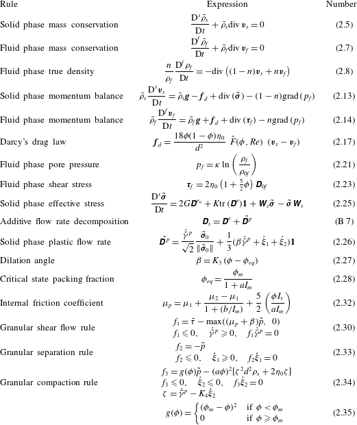
Figure 7 shows the basic method we implement. First, the mixture problem is defined and the material configurations are given (figure 7 a). The two phases are then separated into the continuum bodies described in figure 2 (figure 7 b). These continuum bodies are discretized into continuum ‘chunks’ defined by two sets of Lagrangian material point tracers. These tracers carry the full description of the continuum bodies (e.g. stress, density, velocity) and advect material information through space (figure 7 c). These two sets of tracers are then placed into a simulation domain which is discretized into a background grid. The background grid is where the equation of motion are solved in the weak form (figure 7 d).

Figure 7.

Solving mixture problems using the material point method. (a) Define the mixture and initial configuration including densities, porosities, stresses. (b) Define the solid and fluid phase continuum bodies. (c) Break the continuum bodies into piecewise-defined blocks of material represented by discrete material points. (d) Solve the equations of motion for the mixture on a background grid according to the material point method algorithm described in § C.2.

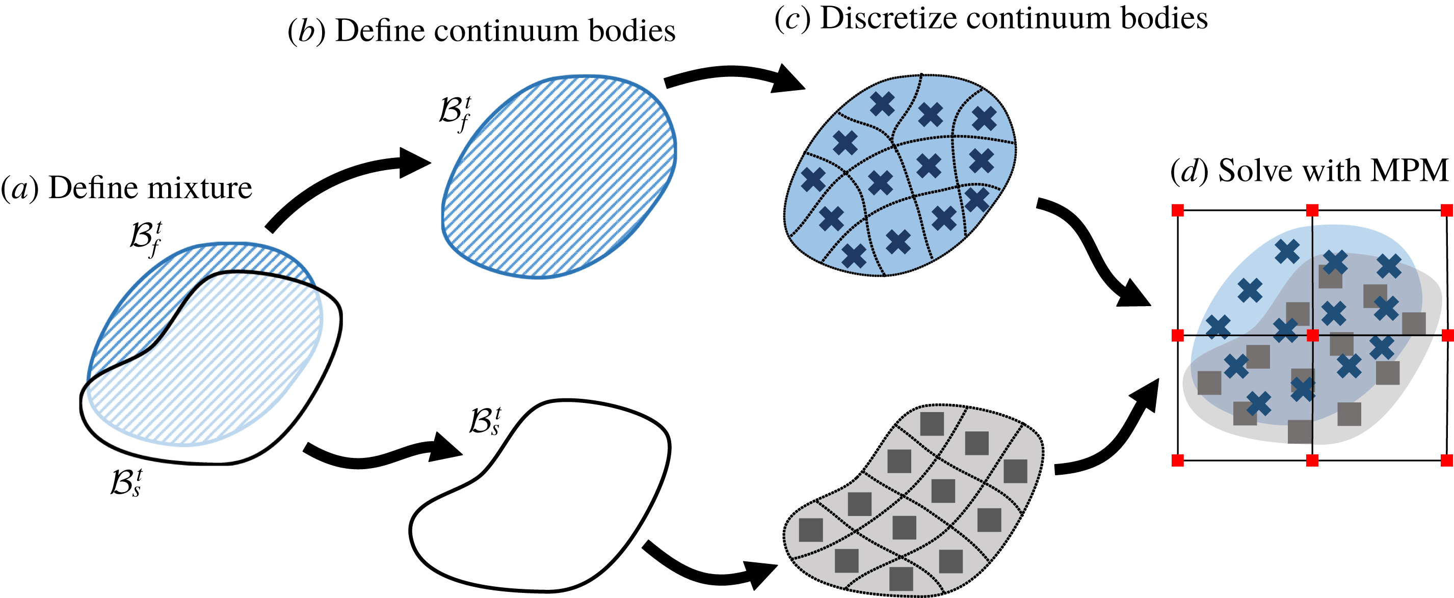
Time integration of the mixture problem is achieved by using an explicit time-marching algorithm. During each discrete time step, the mixture state (stored on the two sets of material points) is projected to the nodes which define the background Cartesian grid. A finite-element-like step is performed which solves the system of equations in table 3 and updates the nodal representation of the mixture velocities and acceleration. These accelerations and velocities are then used to update the mixture state (as stored on the two sets of material points). At the end of the time step, the grid is reset, and the procedure is repeated. In this way, we track the state of the mixture on a moving set of material point tracers and solve the equations of motion of a background finite-element-like grid. Specific details about our implementation of this framework, boundary conditions and novel numerical corrections can be found in appendix B.

5 Results

To validate our model, we use the numerical method described in § 4 to simulate underwater column collapses and quasi-two-dimensional erosion flows for comparison with experimental data reported by Rondon, Pouliquen & Aussillous (Reference Rondon, Pouliquen and Aussillous2011) and Allen & Kudrolli (Reference Allen and Kudrolli2017). We also explore two applications of our method for potential use in impact/penetration problems (as explored in Ceccato et al. (Reference Ceccato, Beuth, Vermeer and Simonini2016)) or for loaded slope failures (see summary of numerical work in this area by Soga et al. (Reference Soga, Alonso, Yerro, Kumar and Bandara2015)).

5.1 Numerical validation of model and method

In this section, we show that our model parameters can be fit to a particular class of fluid–sediment mixtures (in this case glass beads immersed in oil/water mixtures, see Pailha & Pouliquen (Reference Pailha and Pouliquen2009)) and that these fit parameters can be used to accurately simulate an underwater column collapse (from Rondon et al. Reference Rondon, Pouliquen and Aussillous2011) and quasi-two-dimensional erosion flows (from Allen & Kudrolli Reference Allen and Kudrolli2017).

5.1.1 Model fit to glass beads

Pailha & Pouliquen (Reference Pailha and Pouliquen2009) characterize the behaviour of glass beads flowing down a chute while immersed in a viscous fluid (set-up shown in figure 8). The glass beads have density $\unicode[STIX]{x1D70C}_{s}=2500~\text{kg}~\text{m}^{-3}$ and diameter $d=160~\unicode[STIX]{x03BC}\text{m}$ . Two mixtures of water/oil are reported and have viscosities $\unicode[STIX]{x1D702}_{0}=9.8\times 10^{-3}~\text{Pa}~\text{s}$ and $\unicode[STIX]{x1D702}_{0}=96\times 10^{-3}~\text{Pa}~\text{s}$ .

Figure 8.

Experimental geometry used by Pailha & Pouliquen (Reference Pailha and Pouliquen2009). A bed of glass beads is immersed in a tank of viscous fluid. The incline of the base of the tank, $\unicode[STIX]{x1D703}$ , is changed to induce submerged slope avalanches.

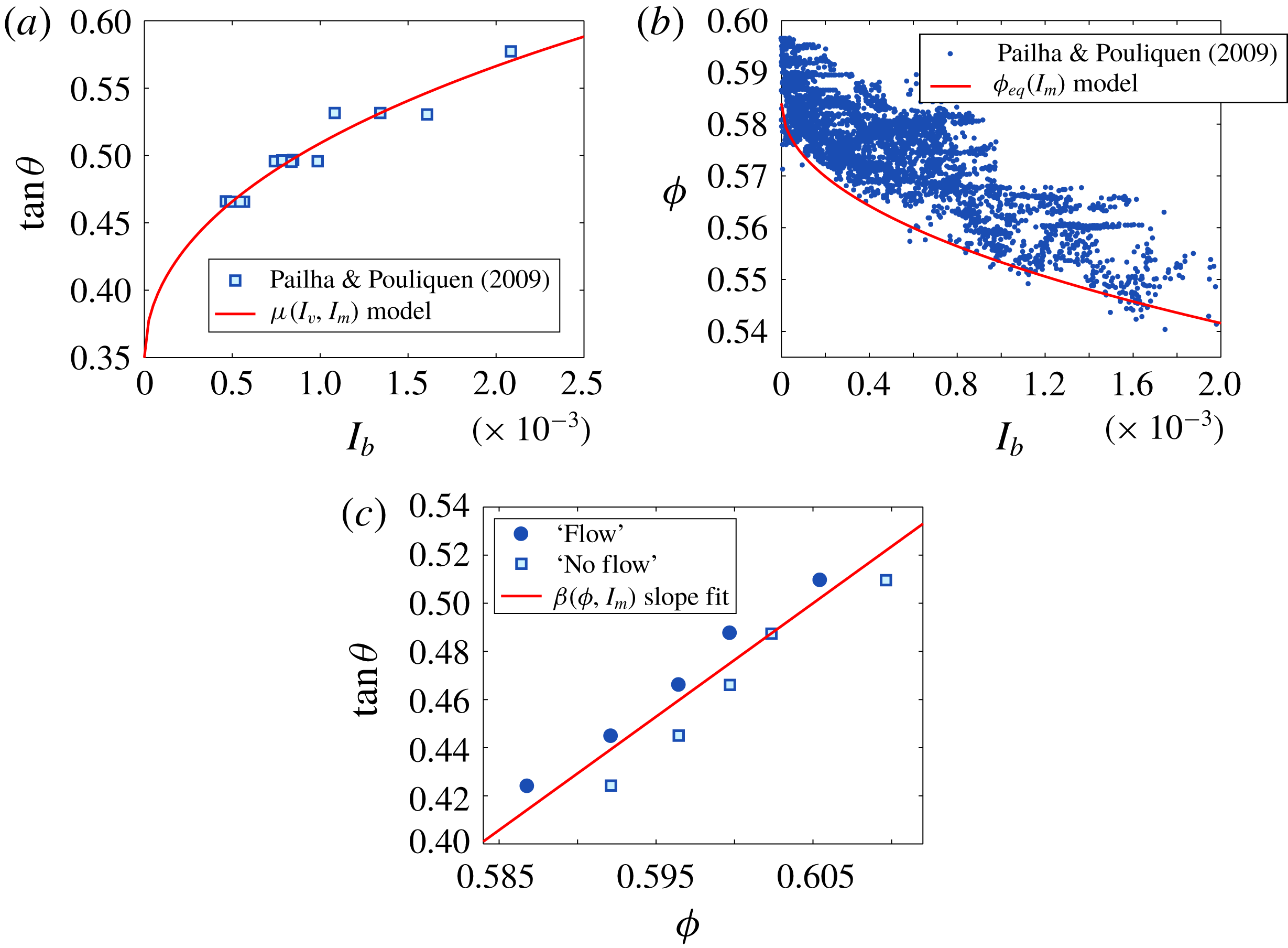
In order to fit our model to the characterization of this mixture, we have focused on a subset of the reported data shown in figure 9. Figure 9(b) shows the measured packing fraction of numerous flows/times plotted against the inertial number $I_{b}$ (defined in Pailha & Pouliquen (Reference Pailha and Pouliquen2009)). We assume that the chute flow profile is parabolic (as is proven in Cassar, Nicolas & Pouliquen (Reference Cassar, Nicolas and Pouliquen2005)) such that $I_{b}\approx I_{v}$ . We further assume that all of the reported flows are in the low Stokes limit $(St\rightarrow 0)$ such that $I_{m}\approx \sqrt{2I_{b}}$ . Fitting (2.28) to the lower extrema of the data, we find the following material parameters,

(5.1a,b )

$$\begin{eqnarray}\unicode[STIX]{x1D719}_{m}=0.584,\quad a=1.23.\end{eqnarray}$$

Figure 9(a) shows the measured internal friction angle $\tan (\unicode[STIX]{x1D703})$ plotted against the experimental inertial number $I_{b}$ . Assuming that all measurements were taken when the flows had reached steady state, $\tan (\unicode[STIX]{x1D703})\approx \unicode[STIX]{x1D707}$ with $\unicode[STIX]{x1D707}$ given in (3.9). Fitting this equation to the data, we find the following material parameters,

(5.2a-c )

$$\begin{eqnarray}\unicode[STIX]{x1D707}_{1}=0.35,\quad \unicode[STIX]{x1D707}_{2}=1.387,\quad b=0.3085.\end{eqnarray}$$

Figure 9(c) shows a set of flow onset measurements. At the transition from the ‘No flow’ state to the ‘Flow’ state, $\tan (\unicode[STIX]{x1D703})\approx \unicode[STIX]{x1D707}_{1}+\unicode[STIX]{x1D6FD}$ . We assume that near the onset of flow $I_{m}=0$ . Therefore, the slope of the transition line between flowing and non-flowing behaviour will be given by $K_{3}$ , and since the rate of compaction in these flows is small (the $K_{4}$ term), we let,

(5.3a,b )

$$\begin{eqnarray}K_{3}=4.715,\quad K_{4}=0.\end{eqnarray}$$

With the parameters above determined for glass beads, we can now simulate other experiments which use similar mixtures. The remaining parameters ( $\unicode[STIX]{x1D70C}_{s}$ , $\unicode[STIX]{x1D70C}_{0f}$ , $\unicode[STIX]{x1D702}_{0}$ and $d$ ) are determined by the specific materials used in the relevant experiments.

Figure 9.

Model fit to the experimental data presented in figure 5 of Pailha & Pouliquen (Reference Pailha and Pouliquen2009). (a) Plot of internal friction coefficient against inertial number. (b) Critical state packing fraction fit to extreme measurements of $\unicode[STIX]{x1D719}$ at various flow rates. (c) $\unicode[STIX]{x1D6FD}$ slope coefficient $K_{3}$ and $K_{4}$ fit to the critical angle between flowing and static slopes.

5.1.2 Granular column collapse of glass beads

Rondon et al. (Reference Rondon, Pouliquen and Aussillous2011) explore the behaviour of collapsing granular columns submerged in a fluid with viscosity $\unicode[STIX]{x1D702}_{0}=12$ or 23 cP and density $\unicode[STIX]{x1D70C}_{0f}\approx 1000~\text{kg}~\text{m}^{-3}$ . A bed of glass beads with diameter $d=225~\unicode[STIX]{x03BC}\text{m}$ and density $\unicode[STIX]{x1D70C}_{s}=2500~\text{kg}~\text{m}^{-3}$ was held at some initial packing fraction behind a retaining wall (see figure 10). Once the wall was removed, the dynamics of the column was measured and reported.

In this work, we are interested in the behaviour of two of the columns reported in that work. The two columns are made of the same mass of glass beads and formed into a loose column and a dense column. The loose column has initial height $h_{0}=4.8$ cm, initial width $l_{0}=6.0$ cm and initial packing fraction $\unicode[STIX]{x1D719}_{0}=0.55$ . The dense column has initial height $h_{0}=4.2$ cm, initial width $l_{0}=6.0$ cm, and initial packing fraction $\unicode[STIX]{x1D719}_{0}=0.60$ . Both columns are immersed in a fluid tank measuring $70~\text{cm}\times 15~\text{cm}\times 15~\text{cm}$ . It was observed that the initially loose column collapsed much faster with much longer run-out than the initially dense column.

Figure 10.

The experimental set-up used by Rondon et al. (Reference Rondon, Pouliquen and Aussillous2011). A column of small glass spheres with initial packing fraction $\unicode[STIX]{x1D719}_{0}$ is held in place by a retaining wall and immersed in a long tank filled with a viscous fluid. At time $t_{0}$ , the wall is removed and the column is allowed to collapse. A pressure sensor at the base of the column (2 cm from the edge of the tank) collects pore pressure data during the collapse. The run-out profiles of the column are captured with a camera.

To simulate these two column collapses, we consider a reduced computational domain by assuming that the flow is approximately plane strain (quasi-two-dimensional) and that the fluid tank can be shortened to 30 cm in length and 10 cm in height without significantly affecting the dynamics of the column collapse (we let the fluid partially fill the tank to a height of 8 cm). We then run our model with the same initial conditions as described in Rondon et al. (Reference Rondon, Pouliquen and Aussillous2011), computational parameters given in table 4 and remaining material parameters given in § 5.1.1. The fluid–wall interaction is governed by a simple frictionless boundary condition while the grain–wall interaction is governed by the frictional boundary rule described in § C.4.2.

Figure 11.

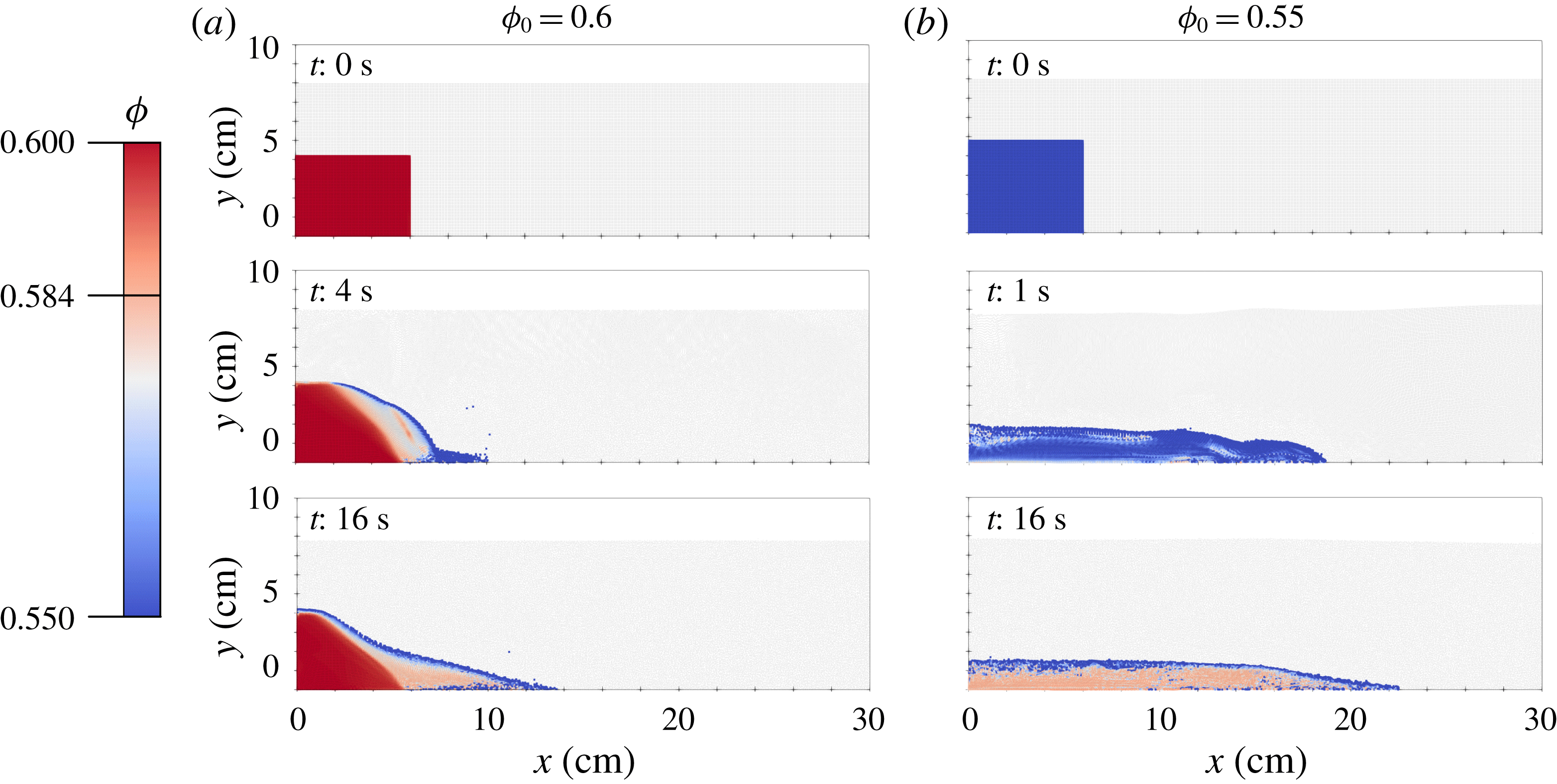
Comparison between simulated collapses for the loose initial packing (b) and the dense initial packing (a) using the $300\times 100$ element grid described in table 4. Solid phase material points are coloured by packing fraction according to the scale at the left. Fluid phase material points are coloured light grey.

Table 4.

Simulation parameters for column collapses run on different grids.

In both the experiments and simulations, the only differences between the dense and loose columns are the initial packing fraction, the initial column height and the initial hydrostatic stress state. The resulting differences in the simulated flow dynamics are due to the different solutions picked out by the governing equations given these initial conditions. A series of snapshots taken from these two simulations (as run on the $300\times 100$ grid) are shown in figure 11; see supplementary movie 1 (available at https://doi.org/10.1017/jfm.2018.914) of these simulations.

In addition to visualizing the solid phase dilation and compaction as in figure 11, we can also examine the differences in shearing rate and fluid pore pressure as shown in figure 12. As the initially dense column collapses, the solid phase experiences shear dilation, increasing the porosity of the mixture. This results in pore tension in the fluid phase as fluid is drawn into the increased pore space (see figure 12 a). This increased pore tension within the collapsing column (as compared to the surrounding fluid) increases the effective granular pressure given by $\tilde{p}$ in (2.31) and therefore strengthens the solid phase resulting in a slower collapse process. On the other hand, as the initially loose column collapses the solid phase experiences plastic compaction, reducing the porosity of the mixture. This has the opposite effect, causing an excess positive pore pressure (see figure 12 b) which reduces the strength of the solid phase. It is this coupling of solid phase flow to fluid phase pressure to solid phase strength that results in these two completely different collapse behaviours.

Figure 12.

Snapshot of simulated solid phase equivalent plastic shear rate (a,b) and fluid phase excess pore pressure (c,d) at $t=4$ s for (a,c) the initially dense column and (b,d) the initially loose column. The plastic shearing rate is visualized at the material point centroids of the solid phase. The post-processed excess pore pressure (see Dunatunga & Kamrin (Reference Dunatunga and Kamrin2015)) as compared to a hydrostatic baseline $p_{eq}$ is visualized at the fluid phase centroids.

By accurately modelling these complex interactions, we are able to capture the vastly different collapse profiles (see figure 13), predict the measured excess pore pressure (see figure 14 a) and match the time-accurate front motion (see figure 14 b) reported in Rondon et al. (Reference Rondon, Pouliquen and Aussillous2011). The collapse profiles shown in figure 13 are the $n=0.45$ contours of the nodal porosity field $n(\boldsymbol{x})$ and show reasonable similarity to the experimental profiles, although there are some artefacts of the finite grid spacing visible near the front of the collapsing column.

Figure 13.

Contours of the collapsing columns from the dense simulation (a) taken at 3 s intervals and the loose simulation (c) taken at 0.66 s intervals. The corresponding contours for the dense experiment (b) and loose experiment (d) from Rondon et al. (Reference Rondon, Pouliquen and Aussillous2011) are also shown. The simulated profiles are generated by plotting the contour of the nodal porosity field (given by the coefficients $\{n_{i}\}$ ) at $n=0.45$ .

The pore pressure in figure 14(b) shows the weighted average nodal representation of pressure (as defined in Dunatunga & Kamrin (Reference Dunatunga and Kamrin2015)) near (but not at) the lower domain boundary and 2 cm from the left wall. This value is compared to a hydrostatic reference value to find the excess pore pressure. In the dense $300\times 100$ simulation, the fluid phase material points exhibited excessive clumping (see § C.4.5), so a second nodal sample was taken at the same height, 2 cm from the right wall and used as the reference value. The front positions shown in figure 14(b) are determined by taking the maximum $x$ -position of the collapse profiles shown in figure 13.

The time history of the simulated pore pressures in figure 14 show close agreement to the experimental measurements; however, the dense simulations appear to saturate at a negative excess pore pressure. This discrepancy is likely due to the high frequency error observed in the MPM stress field before nodal averaging (see Dunatunga & Kamrin (Reference Dunatunga and Kamrin2015)). Mast et al. (Reference Mast, Mackenzie-Helnwein, Arduino, Miller and Shin2012) propose several methods of mitigating these errors and the associated kinematic locking, but we do not implement them here. Altogether, the results shown in figures 13 and 14 indicate that our model is capable of accurately predicting the dynamics of submerged granular column collapses and captures the sensitivity of the problem to small changes in initial conditions.

Figure 14.

(a) Comparison of the simulated excess pore pressure for the loose initial packing (top, blue) and the dense initial packing (bottom, red). The base pore pressure for all simulations is approximately 800 Pa. (b) Comparison between simulated front positions for the loose initial packing (top, blue) and the dense initial packing (bottom, red).

5.1.3 Quasi-two-dimensional flow of glass beads

In addition to sudden collapses of granular columns, we are also interested in using our model to simulate steady erosion processes. To gage the accuracy of our method for such problems, we simulate the experiments performed by Allen & Kudrolli (Reference Allen and Kudrolli2017). As shown in figure 15, the experimental set-up, approximates a two-dimensional (2-D) erosion flow by driving a conical motor at a prescribed rotation rate, $f$ , above an immersed granular bed of glass beads. The fields reported, obtained using index-matching, are a function of vertical depth below the driving surface, $z$ .

Figure 15.

(a) Experimental set-up of Allen & Kudrolli (Reference Allen and Kudrolli2017). An approximately 9 mm bed of grains is immersed in a cylindrical tank filled with fluid. A conical driver is submerged to the granular surface and driven by a motor at a specified rotation rate $f$ . (b) The resulting flow is imaged at a plane near the edge of the tank. Measurements are taken of phase velocities and packing fractions as a function of distance $z$ from the driving surface.

The mixture of fluid and grains used in Allen & Kudrolli (Reference Allen and Kudrolli2017) is similar to that used in Pailha & Pouliquen (Reference Pailha and Pouliquen2009), suggesting that we can use the same material parameters determined in § 5.1.1. The remaining material parameters are given by the specific materials used in the experiment: $\unicode[STIX]{x1D70C}_{0f}=1002~\text{kg}~\text{m}^{-3}$ , $\unicode[STIX]{x1D702}_{0}=0.021$ Pa s, $\unicode[STIX]{x1D70C}_{s}=2500~\text{kg}~\text{m}^{-3}$ and $d=1.05$ mm.

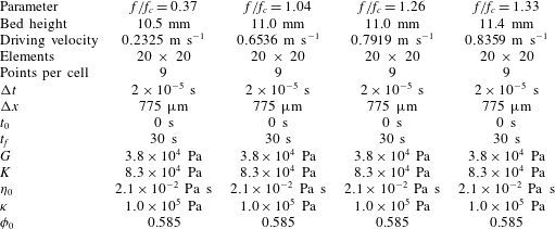
We simulate four of the reported flows in that work, $f/f_{c}=\{0.37,1.04,1.26,1.33\}$ , where $f$ is the assigned driving frequency and $f_{c}$ is the reported critical driving frequency around which grains become suspended in the fluid flow. We set up an $x$ -periodic domain measuring $15.5~\text{mm}\times 15.5~\text{mm}$ and drive the upper surface at a velocity determined by the ratios the driving frequency $f$ . We let the lower wall be governed by a no-slip boundary condition. The resulting fluid flow is allowed to reach steady state and the flow properties are averaged over a 12 s time window. A summary of the simulation set-up is given in table 5.

Table 5.

Simulation parameters for four erosion flows run at different driving velocities.

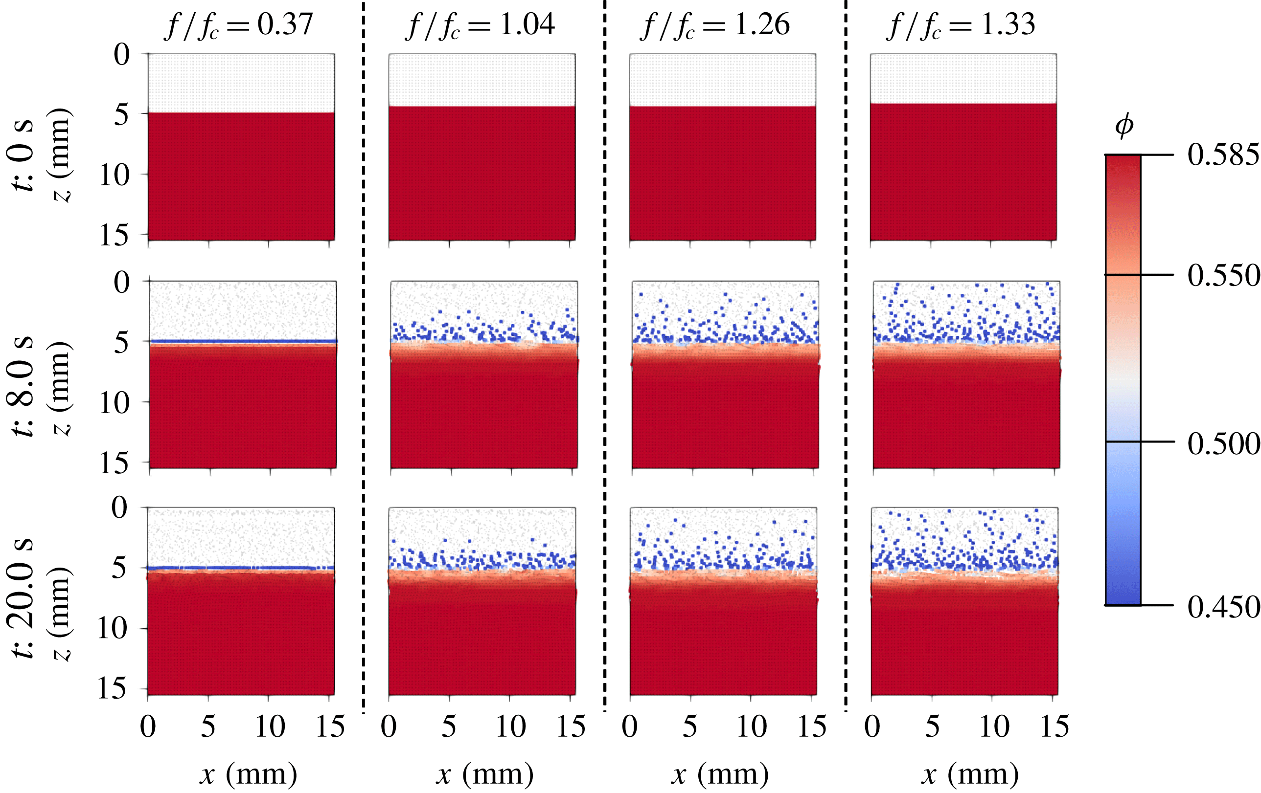
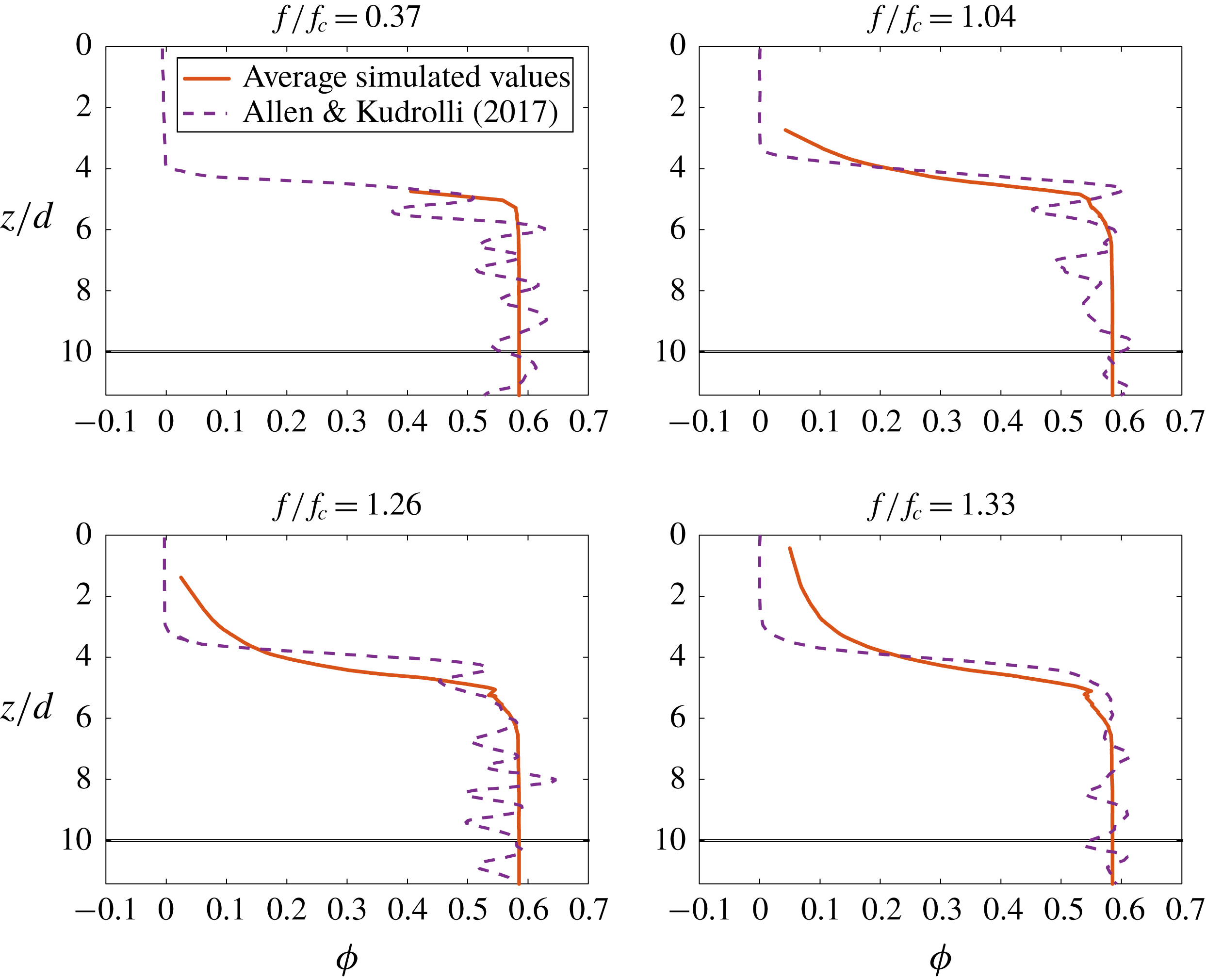
A series of simulation snapshots is shown in figure 16; see supplementary movie 2 to view a video of these simulations. As was observed in Allen & Kudrolli (Reference Allen and Kudrolli2017), below the critical driving frequency $f_{c}$ there is essentially no flow of grains; however, once the driving frequency $f$ is increased above $f_{c}$ , solid phase material is ‘picked up’ by the shearing of the fluid phase and enters into suspension. The steady-state flow predicted by our simulations shows strong similarity to the experimentally measured packing fraction (see figure 17) and phase velocities (see figure 18).

The simulated packing fractions and velocities are plotted by averaging the material point coefficients over a 12 s window. The resulting phase velocity and packing fraction averages are then sorted by the average material point centroid position and filtered using the MATLAB smooth() function. It is important to note that as the solid phase dilates, the solid phase material points will separate. After the material points separate by more than 1 element (around $\unicode[STIX]{x1D719}\approx 0.2$ ), the material point value $\unicode[STIX]{x1D719}_{p}$ will no longer be representative of the true mixture packing fraction.

Figure 16.

Comparison between the simulated erosion flows described in table 5. Solid phase material points are coloured by packing fraction according to the scale at the right. Fluid phase material points are coloured light grey. In all cases, the shearing of the fluid phase induces motion in the solid phase. As the driving frequency $f$ increases above the critical $f_{c}$ (as reported in Allen & Kudrolli (Reference Allen and Kudrolli2017)) solid phase material is ‘picked up’ and becomes suspended in the fluid.

Figure 17.

Plots comparing the time-averaged steady-state packing fractions as a function of normalized depth reported in Allen & Kudrolli (Reference Allen and Kudrolli2017) to those found by running the simulations described in table 5. Very close matching is observed when the solid phase material is dense; however the simulated data have a heavy tail in the dilute regime. This is likely due to the large empty spaces between the solid phase material points when they become suspended in the fluid flow.

Figure 18.

Plots comparing the time-averaged steady-state phase velocities $u$ (normalized by the velocity of the driving surface $u_{t}$ ) as a function of normalized depth reported in Allen & Kudrolli (Reference Allen and Kudrolli2017) to those found by running the simulations described in table 5. The simulated values show strong similarity to the experimental values; however, there are oscillations visible in the simulated profiles. These oscillations are due to well-known errors in the material point velocity fields.

5.2 Qualitative results

In this section we consider two potential applications of our model and method. The first shows the behaviour of a fluid–grain mixture as an intruding body is pressed into its surface. The second shows the effect of water level on the failure of a loaded slope.

5.2.1 Two-dimensional circular intruder

The use of the material point method for intrusion into a saturated soil is explored at length in Ceccato et al. (Reference Ceccato, Beuth, Vermeer and Simonini2016). In that work, the mixture model developed in Bandara & Soga (Reference Bandara and Soga2015) is adjusted to use the Modified Cam Clay model to model the solid phase behaviour.

Here we show that our model may be extended to explore similar problems by simulating the intrusion of a disk into a submerged bed of acrylic beads. As an exploratory problem, we use the material parameters given in table 2 and let $d=1.0$ cm, $\unicode[STIX]{x1D70C}_{s}=2500~\text{kg}~\text{m}^{-3}$ and $\unicode[STIX]{x1D70C}_{f}=1000~\text{kg}~\text{m}^{-3}$ . A $1~\text{m}\times 1~\text{m}$ domain is simulated on a $100\times 100$ element grid with four material points per cell. The domain is initially half-filled by a mixture of fluid and grains with packing fraction $\unicode[STIX]{x1D719}_{0}=0.60$ . 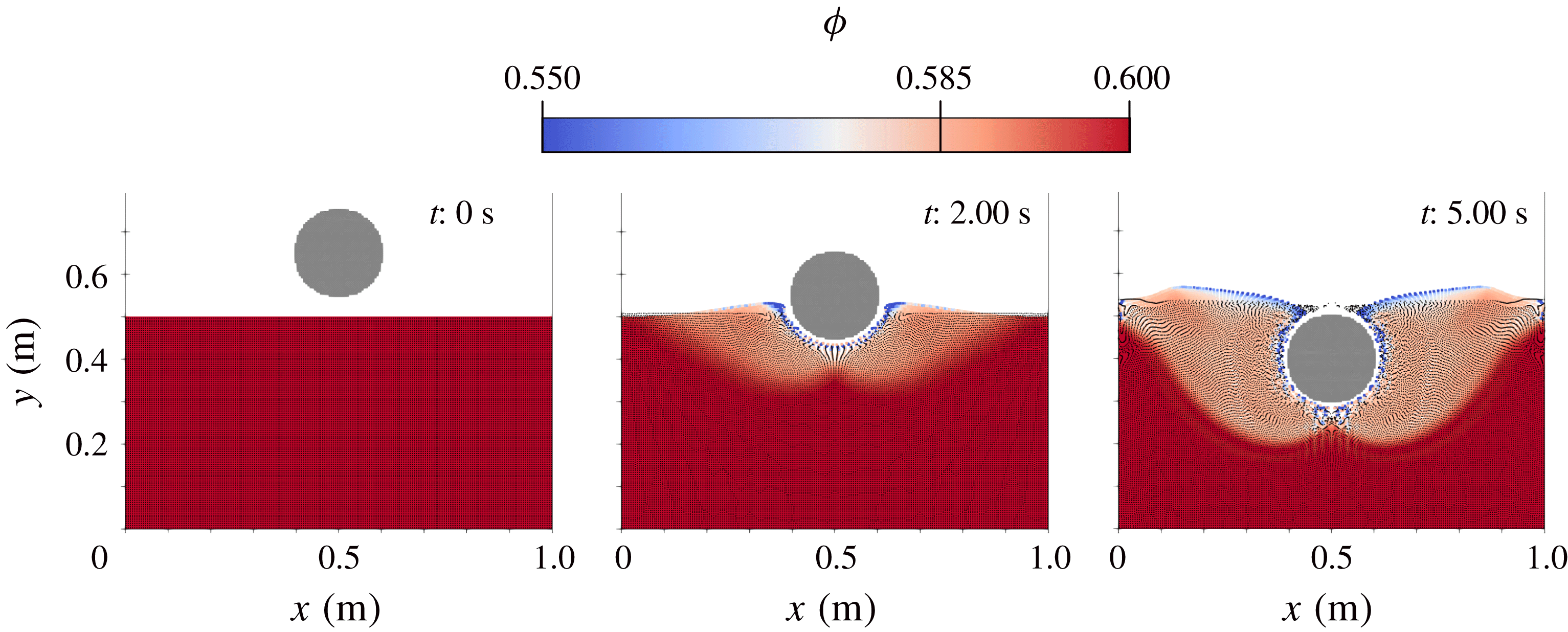The resulting behaviour is shown in figure 19; see supplementary materials for a movie of this simulation. As the intruder enters the mixture, we observe shear dilation of the granular material and independent motion of the two phases of material as fluid fills in the opening pore space under the intruder, revealing dry granular media at the free surface.

Figure 19.

Series of snapshots taken from simulation described in § 5.2.1. Solid phase material points are coloured according to packing fraction. Fluid material points are represented by small black dots. Intruder material points are coloured light grey. As the intruder enters the mixture, the shearing of the solid phase results in noticeable dilation.

5.2.2 Two-dimensional slope collapse

Another application of interest for our model is the complex interactions between structures and saturated soils. To demonstrate the application of this model to the problem of a loaded slope, we consider two simple cases. In the first case, a dry slope with length 14 m and height 5 m is loaded with a cement block at the top (see figure 20). The slope is composed of 2 mm diameter grains with density $\unicode[STIX]{x1D70C}_{s}=2500~\text{kg}~\text{m}^{-3}$ . In the second case, an identical slope with identical loading and material composition is partially submerged in water (approximating a shoreline).

The simulations are performed in a $40~\text{m}\times 10~\text{m}$ domain discretized into $160\times 40$ elements. The material points for the three bodies are seeded with nine material points per grid cell. The initial packing of the granular slope is $\unicode[STIX]{x1D719}_{0}=0.585$ . The resulting collapses are shown in figure 20; see supplemental Movie4 to view a movie of these simulations. We let the material properties be identical to those given in § 5.1.1. As shown in figure 21, the resulting motion of the block (approximating a structure) on top of the slope has a strong dependence on the water lever in the slope. Over the course of 5 simulated seconds, the block on the partially submerged slope moves 20 % more in the $x$ -direction, 36 % more in the $y$ -direction and rotates 34 % less.

Figure 20.

Series of snapshots taken from simulations described in § 5.2.2. Solid phase material points are coloured according to the equivalent plastic shearing rate, $\dot{\bar{\unicode[STIX]{x1D6FE}}}^{p}$ . Fluid material points are represented by light grey dots. Block material points are coloured light grey.

Figure 21.

Plots of block motion for simulations described in § 5.2.2. (a) The $x$ -displacement of the block’s centre of mass. (b) The $y$ -displacement of the block’s centre of mass. (c) The rotation of the block about its centre of mass.

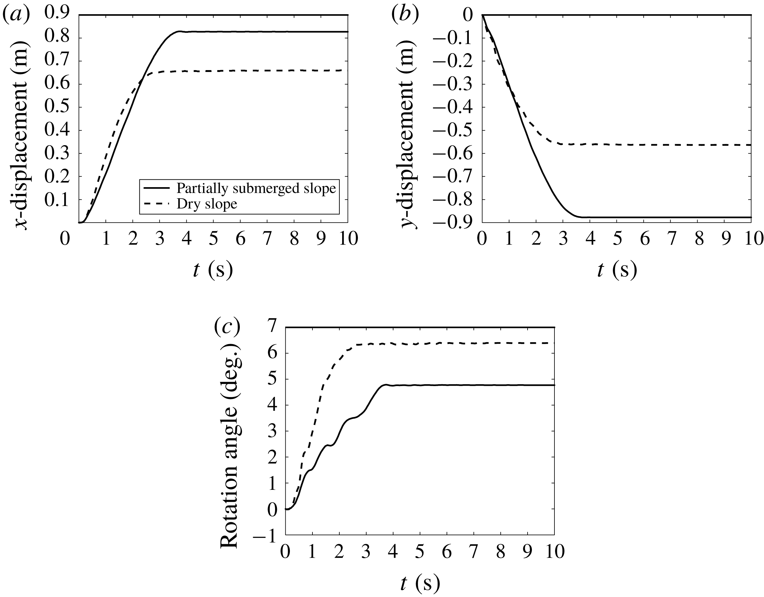
6 Conclusion

We have developed a full set of constitutive relations for fluid–sediment mixtures which is capable of accurately and robustly modelling both dense and dilute flows of material. Our model is derived from a thermodynamically consistent set of rules and formulated to capture the dry and viscous inertial rheologies of granular materials, the critical state behaviour of grains under shear, the change in the effective viscosity of the fluid due to suspended sediments and a robust Darcy-like inter-phase drag. This model is implemented in MPM and validated against experiment. We characterize mixtures of glass beads immersed in a Newtonian fluid by fitting our model to the experimental data reported in Pailha & Pouliquen (Reference Pailha and Pouliquen2009). We then take these material parameters and show that our model is able to accurately predict the behaviour of both collapsing granular columns (see Rondon et al. Reference Rondon, Pouliquen and Aussillous2011) and shearing of fluid above granular beds (see Allen & Kudrolli Reference Allen and Kudrolli2017) without re-fitting material properties. In addition, we also look at the application of this model and method to the problems of intrusion and slope stability.

The model we have presented in this work may be extensible to more general fluid–sediment mixtures such as those involving air (especially for examining the kick-up of dust for vertical take-off and landing vehicles). Other extensions of this model may look at adding cohesion (redefining the $f_{1}$ and $f_{2}$ yield conditions), introducing a fabric tensor to the rules governing dilation or adding non-local effects (Kamrin & Koval Reference Kamrin and Koval2012; Henann & Kamrin Reference Henann and Kamrin2013; Kamrin & Henann Reference Kamrin and Henann2015) to capture, for example, the exponential-type decay of the granular velocity field deep in fluid-driven beds (Houssais et al. Reference Houssais, Ortiz, Durian and Jerolmack2015; Allen & Kudrolli Reference Allen and Kudrolli2017).

Acknowledgements

This work was supported by Army Research Office grant W911NF-16-1-0440 and National Science Foundation grant CBET-1253228. We thank P. Aussilous for access to experimental data from Rondon et al. (Reference Rondon, Pouliquen and Aussillous2011).

Supplementary movies

Supplementary movies are available at https://doi.org/10.1017/jfm.2018.914.

Appendix A

The constitutive rules for our material model given in table 1 are derived in the following specialization of the two-phase thermodynamic analysis from Drumheller (Reference Drumheller2000). The basic rules for our model are similar to those described in Coussy (Reference Coussy2004); however, our derivation allows for two mixture temperatures, $\unicode[STIX]{x1D717}_{s}$ and $\unicode[STIX]{x1D717}_{f}$ , and (as mentioned previously) we do not explicitly account for tortuosity.

A.1 First law of thermodynamics

The first law of thermodynamics states that the rate of change of the total energy stored within a volume must be equal to the rate of heat flow into the volume plus the external power exerted on the volume. The total energy stored within a volume is the sum of internal energy and kinetic energy. We define a local expression for the energy conservation in the mixture in terms of the specific internal energies $\unicode[STIX]{x1D700}_{s}$ and $\unicode[STIX]{x1D700}_{f}$ , the phase-wise external heat fluxes $\boldsymbol{q}_{s}$ and $\boldsymbol{q}_{f}$ , the phase-wise internal heat generation $q_{s}$ and $q_{f}$ and the basic homogenized continuum fields from § 2.1.1,

(A 1)

$$\begin{eqnarray}\displaystyle & & \displaystyle \bar{\unicode[STIX]{x1D70C}}_{s}\frac{\text{D}^{s}\unicode[STIX]{x1D700}_{s}}{\text{D}t}+\bar{\unicode[STIX]{x1D70C}}_{f}\frac{\text{D}^{f}\unicode[STIX]{x1D700}_{f}}{\text{D}t}+\bar{\unicode[STIX]{x1D70C}}_{s}\frac{\text{D}^{s}\boldsymbol{v}_{s}}{\text{D}t}\boldsymbol{\cdot }\boldsymbol{v}_{s}+\bar{\unicode[STIX]{x1D70C}}_{f}\frac{\text{D}^{f}\boldsymbol{v}_{f}}{\text{D}t}\boldsymbol{\cdot }\boldsymbol{v}_{f}\nonumber\\ \displaystyle & & \displaystyle \quad =(\text{div}\,(\unicode[STIX]{x1D748}_{s})+\bar{\unicode[STIX]{x1D70C}}_{s}\boldsymbol{g})\boldsymbol{\cdot }\boldsymbol{v}_{s}+(\text{div}\,(\unicode[STIX]{x1D748}_{f})+\bar{\unicode[STIX]{x1D70C}}_{f}\boldsymbol{g})\boldsymbol{\cdot }\boldsymbol{v}_{f}\nonumber\\ \displaystyle & & \displaystyle \qquad +\,\unicode[STIX]{x1D748}_{s}\boldsymbol{ : }\text{grad}\,(\boldsymbol{v}_{s})+\unicode[STIX]{x1D748}_{f}\boldsymbol{ : }\text{grad}\,(\boldsymbol{v}_{f})\nonumber\\ \displaystyle & & \displaystyle \qquad +\,q_{s}+q_{f}-\text{div}\,(\boldsymbol{q}_{s}+\boldsymbol{q}_{f})\end{eqnarray}$$

which, with the momentum balance expressions in (2.9), the buoyant force from (2.10), the specific form of the phase stresses in (2.11) and (2.12) and the evolution law for the true fluid density from (2.8), becomes,

(A 2)

$$\begin{eqnarray}\displaystyle \bar{\unicode[STIX]{x1D70C}}_{s}\frac{\text{D}^{s}\unicode[STIX]{x1D700}_{s}}{\text{D}t}+\bar{\unicode[STIX]{x1D70C}}_{f}\frac{\text{D}^{f}\unicode[STIX]{x1D700}_{f}}{\text{D}t} & = & \displaystyle p_{f}\left(\frac{n}{\unicode[STIX]{x1D70C}_{f}}\frac{\text{D}^{f}\unicode[STIX]{x1D70C}_{f}}{\text{D}t}\right)+\boldsymbol{f}_{d}\boldsymbol{\cdot }(\boldsymbol{v}_{s}-\boldsymbol{v}_{f})\nonumber\\ \displaystyle & & \displaystyle +\,\tilde{\unicode[STIX]{x1D748}}\boldsymbol{ : }\text{grad}\,(\boldsymbol{v}_{s})+\unicode[STIX]{x1D749}_{f}\boldsymbol{ : }\text{grad}\,(\boldsymbol{v}_{f})\nonumber\\ \displaystyle & & \displaystyle +\,q_{s}+q_{f}-\text{div}\,(\boldsymbol{q}_{s}+\boldsymbol{q}_{f}).\end{eqnarray}$$

A.2 Second law of thermodynamics

The second law of thermodynamics states that the rate of change of the total entropy within a volume $\unicode[STIX]{x1D6FA}$ must always be greater than or equal to the combined entropy flow into the volume. Drumheller (Reference Drumheller2000) gives the following necessary condition for entropy imbalance of a mixture,

(A 3)

$$\begin{eqnarray}\bar{\unicode[STIX]{x1D70C}}_{s}\frac{\text{D}^{s}s_{s}}{\text{D}t}+\bar{\unicode[STIX]{x1D70C}}_{f}\frac{\text{D}^{f}s_{f}}{\text{D}t}+\text{div}\left(\frac{\boldsymbol{q}_{s}}{\unicode[STIX]{x1D717}_{s}}+\frac{\boldsymbol{q}_{f}}{\unicode[STIX]{x1D717}_{f}}\right)-\frac{q_{s}}{\unicode[STIX]{x1D717}_{s}}-\frac{q_{f}}{\unicode[STIX]{x1D717}_{f}}\geqslant 0.\end{eqnarray}$$

We add two additional conditions by considering the entropy flow into each phase separately including the entropy flow due to the inter-phase heat flow $q_{i}$ ,

(A 4)

$$\begin{eqnarray}\displaystyle \left.\begin{array}{@{}c@{}}\displaystyle \bar{\unicode[STIX]{x1D70C}}_{s}\frac{\text{D}^{s}s_{s}}{\text{D}t}+\text{div}\left(\frac{\boldsymbol{q}_{s}}{\unicode[STIX]{x1D717}_{s}}\right)-\frac{q_{s}-q_{i}}{\unicode[STIX]{x1D717}_{s}}\geqslant 0\\ \displaystyle \bar{\unicode[STIX]{x1D70C}}_{f}\frac{\text{D}^{f}s_{f}}{\text{D}t}+\text{div}\left(\frac{\boldsymbol{q}_{f}}{\unicode[STIX]{x1D717}_{f}}\right)-\frac{q_{f}+q_{i}}{\unicode[STIX]{x1D717}_{f}}\geqslant 0.\end{array}\right\} & & \displaystyle\end{eqnarray}$$

In the absence of inter-phase heat flow, satisfying the conditions in (A 4) also necessarily satisfies (A 3). Combining these last two expressions we find a second condition for entropy balance which does not depend on the inter-phase heat flow, $q_{i}$ .

(A 5)

$$\begin{eqnarray}\bar{\unicode[STIX]{x1D70C}}_{s}\unicode[STIX]{x1D717}_{s}\frac{\text{D}^{s}s_{s}}{\text{D}t}+\bar{\unicode[STIX]{x1D70C}}_{f}\unicode[STIX]{x1D717}_{f}\frac{\text{D}^{f}s_{f}}{\text{D}t}-\left(\frac{\boldsymbol{q}_{s}\boldsymbol{\cdot }\text{grad}\,(\unicode[STIX]{x1D717}_{s})}{\unicode[STIX]{x1D717}_{s}}+\frac{\boldsymbol{q}_{f}\boldsymbol{\cdot }\text{grad}\,(\unicode[STIX]{x1D717}_{f})}{\unicode[STIX]{x1D717}_{f}}\right)+\text{div}\,(\boldsymbol{q}_{s}+\boldsymbol{q}_{f})-(q_{s}+q_{f})\geqslant 0.\end{eqnarray}$$

A.3 Helmholtz free energy

We now introduce the definition for the phase-wise Helmholtz free energies, $\unicode[STIX]{x1D713}_{s}$ and $\unicode[STIX]{x1D713}_{f}$ , such that,

(A 6)

$$\begin{eqnarray}\left.\begin{array}{@{}c@{}}\unicode[STIX]{x1D713}_{s}=\unicode[STIX]{x1D700}_{s}-s_{s}\unicode[STIX]{x1D717}_{s}\\ \unicode[STIX]{x1D713}_{f}=\unicode[STIX]{x1D700}_{f}-s_{f}\unicode[STIX]{x1D717}_{f}.\end{array}\right\}\end{eqnarray}$$

Substituting into the first law expression in (A 2) and combining with the second law expression from (A 5), the following free energy inequality is found,

(A 7)

$$\begin{eqnarray}\displaystyle 0 & {\leqslant} & \displaystyle -\bar{\unicode[STIX]{x1D70C}}_{s}\frac{\text{D}^{s}\unicode[STIX]{x1D713}_{s}}{\text{D}t}-\bar{\unicode[STIX]{x1D70C}}_{f}\frac{\text{D}^{f}\unicode[STIX]{x1D713}_{f}}{\text{D}t}-\bar{\unicode[STIX]{x1D70C}}_{s}s_{s}\frac{\text{D}^{s}\unicode[STIX]{x1D717}_{s}}{\text{D}t}-\bar{\unicode[STIX]{x1D70C}}_{f}s_{f}\frac{\text{D}^{f}\unicode[STIX]{x1D717}_{f}}{\text{D}t}\nonumber\\ \displaystyle & & \displaystyle +\,p_{f}\left(\frac{n}{\unicode[STIX]{x1D70C}_{f}}\frac{\text{D}^{f}\unicode[STIX]{x1D70C}_{f}}{\text{D}t}\right)+\boldsymbol{f}_{d}\boldsymbol{\cdot }(\boldsymbol{v}_{s}-\boldsymbol{v}_{f})+\tilde{\unicode[STIX]{x1D748}}\boldsymbol{ : }\text{grad}\,(\boldsymbol{v}_{s})\nonumber\\ \displaystyle & & \displaystyle +\,\unicode[STIX]{x1D749}_{f}\boldsymbol{ : }\text{grad}\,(\boldsymbol{v}_{f})-\frac{\boldsymbol{q}_{s}\boldsymbol{\cdot }\text{grad}\,(\unicode[STIX]{x1D717}_{s})}{\unicode[STIX]{x1D717}_{s}}-\frac{\boldsymbol{q}_{f}\boldsymbol{\cdot }\text{grad}\,(\unicode[STIX]{x1D717}_{f})}{\unicode[STIX]{x1D717}_{f}}.\end{eqnarray}$$

We let the spatial solid phase and fluid phase velocity gradients be expressed in matrix form as,

(A 8a,b )

$$\begin{eqnarray}\unicode[STIX]{x1D647}_{s}\equiv \text{grad}\,(\boldsymbol{v}_{s}),\quad \unicode[STIX]{x1D647}_{f}\equiv \text{grad}\,(\boldsymbol{v}_{s}),\end{eqnarray}$$

which have unique decompositions into a phase spin tensor, $\unicode[STIX]{x1D652}$ , and a phase strain-rate tensor, $\unicode[STIX]{x1D63F}$ ,

(A 9a,b )

$$\begin{eqnarray}\unicode[STIX]{x1D63F}=\text{sym}(\unicode[STIX]{x1D647})={\textstyle \frac{1}{2}}(\unicode[STIX]{x1D647}+\unicode[STIX]{x1D647}^{\top }),\quad \text{and}\quad \unicode[STIX]{x1D652}=\text{skw}(\unicode[STIX]{x1D647})={\textstyle \frac{1}{2}}(\unicode[STIX]{x1D647}-\unicode[STIX]{x1D647}^{\top }).\end{eqnarray}$$

We further assume that the solid and fluid phases have uniform and constant temperatures, $\unicode[STIX]{x1D717}_{s}$ and $\unicode[STIX]{x1D717}_{f}$ , such that (A 7) becomes,

(A 10)

$$\begin{eqnarray}-\bar{\unicode[STIX]{x1D70C}}_{s}\frac{\text{D}^{s}\unicode[STIX]{x1D713}_{s}}{\text{D}t}-\bar{\unicode[STIX]{x1D70C}}_{f}\frac{\text{D}^{f}\unicode[STIX]{x1D713}_{f}}{\text{D}t}+p_{f}\left(\frac{n}{\unicode[STIX]{x1D70C}_{f}}\frac{\text{D}^{f}\unicode[STIX]{x1D70C}_{f}}{\text{D}t}\right)+(\tilde{\unicode[STIX]{x1D748}}\boldsymbol{ : }\unicode[STIX]{x1D63F}_{s})+(\unicode[STIX]{x1D749}_{f}\boldsymbol{ : }\unicode[STIX]{x1D63F}_{0f})+\boldsymbol{f}_{d}\boldsymbol{\cdot }(\boldsymbol{v}_{s}-\boldsymbol{v}_{f})\geqslant 0.\end{eqnarray}$$

A.4 Fluid phase free energy function

The conservative constitutive behaviour of the fluid phase is governed by the fluid phase specific free energy, $\unicode[STIX]{x1D713}_{f}$ . We assume that the functional form of the free energy only depends on the true fluid density, $\unicode[STIX]{x1D713}_{f}=\hat{\unicode[STIX]{x1D713}}_{f}(\unicode[STIX]{x1D70C}_{f})$ . Substituting into the expression for free energy imbalance in (A 10),

(A 11)

$$\begin{eqnarray}-\bar{\unicode[STIX]{x1D70C}}_{s}\frac{\text{D}^{s}\unicode[STIX]{x1D713}_{s}}{\text{D}t}+(\tilde{\unicode[STIX]{x1D748}}\boldsymbol{ : }\unicode[STIX]{x1D63F}_{s})-\frac{n}{\unicode[STIX]{x1D70C}_{f}}\frac{\text{D}^{f}\unicode[STIX]{x1D70C}_{f}}{\text{D}t}\left(p_{f}-\unicode[STIX]{x1D70C}_{f}^{2}\frac{\unicode[STIX]{x2202}\hat{\unicode[STIX]{x1D713}}_{f}(\unicode[STIX]{x1D70C}_{f})}{\unicode[STIX]{x2202}\unicode[STIX]{x1D70C}_{f}}\right)+(\unicode[STIX]{x1D749}_{f}\boldsymbol{ : }\unicode[STIX]{x1D63F}_{0f})+\boldsymbol{f}_{d}\boldsymbol{\cdot }(\boldsymbol{v}_{s}-\boldsymbol{v}_{f})\geqslant 0.\end{eqnarray}$$

A.5 Solid phase free energy function

The solid phase behaviour will be governed by an elastic–plastic constitutive relation derived from that given in Anand & Su (Reference Anand and Su2005). We begin with the definition of the solid phase deformation gradient,

(A 12a,b )

$$\begin{eqnarray}\unicode[STIX]{x1D641}=\frac{\unicode[STIX]{x2202}\unicode[STIX]{x1D74C}_{s}(\boldsymbol{X},t)}{\unicode[STIX]{x2202}\boldsymbol{X}},\quad \frac{\text{D}^{s}\unicode[STIX]{x1D641}}{\text{D}t}=\unicode[STIX]{x1D647}_{s}\unicode[STIX]{x1D641},\end{eqnarray}$$

where $\unicode[STIX]{x1D74C}_{s}(\boldsymbol{X},t)$ is the motion function mapping from a position, $\boldsymbol{X}$ , in the solid reference configuration to a position in the solid deformed (current) configuration at time $t$ .

We assume the Kroner–Lee decomposition of the deformation gradient,

(A 13)

$$\begin{eqnarray}\unicode[STIX]{x1D641}=\unicode[STIX]{x1D641}^{e}\unicode[STIX]{x1D641}^{p},\end{eqnarray}$$

with $\unicode[STIX]{x1D641}^{e}$ the elastic deformation and $\unicode[STIX]{x1D641}^{p}$ the plastic deformation. With this, the velocity gradient can be separated into an elastic and plastic flow,

(A 14a-c )

$$\begin{eqnarray}\unicode[STIX]{x1D647}_{s}=\unicode[STIX]{x1D647}^{e}+\unicode[STIX]{x1D641}^{e}\unicode[STIX]{x1D647}^{p}\unicode[STIX]{x1D641}^{e-1},\quad \text{such that }\frac{\text{D}^{s}\unicode[STIX]{x1D641}^{e}}{\text{D}t}=\unicode[STIX]{x1D647}^{e}\unicode[STIX]{x1D641}^{e},\quad \frac{\text{D}^{s}\unicode[STIX]{x1D641}^{p}}{\text{D}t}=\unicode[STIX]{x1D647}^{p}\unicode[STIX]{x1D641}^{p}.\end{eqnarray}$$

We assume that the plastic flow, $\unicode[STIX]{x1D647}^{p}$ , is symmetric such that,

(A 15a-d )

$$\begin{eqnarray}\unicode[STIX]{x1D63F}^{e}=\text{sym}(\unicode[STIX]{x1D647}^{e}),\quad \unicode[STIX]{x1D652}^{e}=\unicode[STIX]{x1D652}_{s},\quad \unicode[STIX]{x1D63F}^{\,p}=\text{sym}(\unicode[STIX]{x1D647}^{p}),\quad \unicode[STIX]{x1D652}^{p}=\mathbf{0}.\end{eqnarray}$$

The right polar decomposition of the elastic deformation is defined as $\unicode[STIX]{x1D641}^{e}=\unicode[STIX]{x1D64D}^{e}\unicode[STIX]{x1D650}^{e}$ , with $\unicode[STIX]{x1D64D}^{e}$ the orthogonal rotation tensor and $\unicode[STIX]{x1D650}^{e}$ the symmetric positive definite elastic stretch tensor. The right Cauchy–Green tensor is then, $\unicode[STIX]{x1D63E}^{e}=\unicode[STIX]{x1D650}^{e^{2}}=\unicode[STIX]{x1D641}^{e\top }\unicode[STIX]{x1D641}^{e}$ . Since $\unicode[STIX]{x1D650}^{e}$ is symmetric and positive definite, it admits a spectral decomposition which we use to define the logarithmic strain tensor, $\unicode[STIX]{x1D640}^{e}$ ,

(A 16a,b )

$$\begin{eqnarray}\unicode[STIX]{x1D650}^{e}=\mathop{\sum }_{i=1}^{3}\unicode[STIX]{x1D706}_{i}\boldsymbol{r}_{i}\otimes \boldsymbol{r}_{i},\quad \text{and}\quad \unicode[STIX]{x1D640}^{e}=\ln (\unicode[STIX]{x1D650}^{e})\equiv \mathop{\sum }_{i=1}^{3}\ln (\unicode[STIX]{x1D706}_{i})\boldsymbol{r}_{i}\otimes \boldsymbol{r}_{i},\end{eqnarray}$$

where $\{\unicode[STIX]{x1D706}_{i}\}$ are the principal stretches, $\{\boldsymbol{r}_{i}\}$ are the right principal directions and each $\unicode[STIX]{x1D706}_{i}>0$ . Further we define the volumetric Jacobians as,

(A 17a-c )

$$\begin{eqnarray}J\equiv \det (\unicode[STIX]{x1D641})>0,\quad J^{e}\equiv \det (\unicode[STIX]{x1D641}^{e})>0,\quad J^{p}\equiv \det (\unicode[STIX]{x1D641}^{p})>0.\end{eqnarray}$$

We introduce the solid phase volumetric free energy, $\unicode[STIX]{x1D711}_{s}$ , which is defined as,

(A 18a,b )

$$\begin{eqnarray}\unicode[STIX]{x1D711}_{s}=J^{e}\bar{\unicode[STIX]{x1D70C}}_{s}\unicode[STIX]{x1D713}_{s},\quad \text{such that }\unicode[STIX]{x1D711}_{s}=\hat{\unicode[STIX]{x1D711}}_{s}(\unicode[STIX]{x1D63E}^{e})=\tilde{\unicode[STIX]{x1D711}}_{s}(\unicode[STIX]{x1D640}^{e}).\end{eqnarray}$$

Therefore (A 11) has the following specialized form,

(A 19)

$$\begin{eqnarray}\displaystyle & & \displaystyle \left(\tilde{\unicode[STIX]{x1D748}}-2J^{e-1}\unicode[STIX]{x1D641}^{e}\frac{\unicode[STIX]{x2202}\hat{\unicode[STIX]{x1D711}}_{s}(\unicode[STIX]{x1D63E}^{e})}{\unicode[STIX]{x2202}\unicode[STIX]{x1D63E}^{e}}\unicode[STIX]{x1D641}^{e\top }\right)\boldsymbol{ : }\unicode[STIX]{x1D63F}^{e}+(\tilde{\unicode[STIX]{x1D748}}\boldsymbol{ : }(\unicode[STIX]{x1D641}^{e}\unicode[STIX]{x1D63F}^{\,p}\unicode[STIX]{x1D641}^{e-1})-(J^{e-1}\unicode[STIX]{x1D711}_{s}\mathbf{1})\boldsymbol{ : }\unicode[STIX]{x1D63F}^{\,p})\nonumber\\ \displaystyle & & \displaystyle \qquad -\,\frac{n}{\unicode[STIX]{x1D70C}_{f}}\frac{\text{D}^{f}\unicode[STIX]{x1D70C}_{f}}{\text{D}t}\left(p_{f}-\unicode[STIX]{x1D70C}_{f}^{2}\frac{\unicode[STIX]{x2202}\hat{\unicode[STIX]{x1D713}}_{f}(\unicode[STIX]{x1D70C}_{f})}{\unicode[STIX]{x2202}\unicode[STIX]{x1D70C}_{f}}\right)+(\unicode[STIX]{x1D749}_{f}\boldsymbol{ : }\unicode[STIX]{x1D63F}_{0f})+\boldsymbol{f}_{d}\boldsymbol{\cdot }(\boldsymbol{v}_{s}-\boldsymbol{v}_{f})\geqslant 0.\end{eqnarray}$$

A.6 Rules for constitutive relations

The expression in (A 19) must be true for all flows everywhere. Since it is possible to conceive of mixture motions with independently varying (and possibly vanishing) values for $\unicode[STIX]{x1D63F}^{e}$ , $\unicode[STIX]{x1D63F}^{\,p}$ , $\text{D}^{s}\unicode[STIX]{x1D70C}_{f}/\text{D}t$ , $\unicode[STIX]{x1D63F}_{0f}$ and $(\boldsymbol{v}_{s}-\boldsymbol{v}_{f})$ , the following relations must each individually be satisfied,

(A 20)

$$\begin{eqnarray}\displaystyle & \displaystyle p_{f}-\unicode[STIX]{x1D70C}_{f}^{2}\frac{\unicode[STIX]{x2202}\hat{\unicode[STIX]{x1D713}}_{f}(\unicode[STIX]{x1D70C}_{f})}{\unicode[STIX]{x2202}\unicode[STIX]{x1D70C}_{f}}=0 & \displaystyle\end{eqnarray}$$

(A 21)

$$\begin{eqnarray}\displaystyle & \displaystyle \unicode[STIX]{x1D749}_{f}\boldsymbol{ : }\unicode[STIX]{x1D63F}_{0f}\geqslant 0 & \displaystyle\end{eqnarray}$$

(A 22)

$$\begin{eqnarray}\displaystyle & \displaystyle \tilde{\unicode[STIX]{x1D748}}-2J^{e-1}\unicode[STIX]{x1D641}^{e}\frac{\unicode[STIX]{x2202}\hat{\unicode[STIX]{x1D711}}_{s}(\unicode[STIX]{x1D63E}^{e})}{\unicode[STIX]{x2202}\unicode[STIX]{x1D63E}^{e}}\unicode[STIX]{x1D641}^{e\top }=0 & \displaystyle\end{eqnarray}$$

(A 23)

$$\begin{eqnarray}\displaystyle & \displaystyle \tilde{\unicode[STIX]{x1D748}}\boldsymbol{ : }(\unicode[STIX]{x1D641}^{e}\unicode[STIX]{x1D63F}^{\,p}\unicode[STIX]{x1D641}^{e-1})-(J^{e-1}\unicode[STIX]{x1D711}_{s}\mathbf{1})\boldsymbol{ : }\unicode[STIX]{x1D63F}^{\,p}\geqslant 0 & \displaystyle\end{eqnarray}$$

(A 24)

$$\begin{eqnarray}\displaystyle & \displaystyle \boldsymbol{f}_{d}\boldsymbol{\cdot }(\boldsymbol{v}_{s}-\boldsymbol{v}_{f})\geqslant 0. & \displaystyle\end{eqnarray}$$

Appendix B

Following the thermodynamic analysis in appendix A, we let the solid phase effective granular stress be given by a stiff elastic specialization of the model derived in Anand & Su (Reference Anand and Su2005).

B.1 Solid phase effective granular stress

Beginning with the equality in (A 22), we define the solid phase effective stress $\tilde{\unicode[STIX]{x1D748}}$ as,

(B 1)

$$\begin{eqnarray}\tilde{\unicode[STIX]{x1D748}}=2J^{e-1}\unicode[STIX]{x1D641}^{e}\frac{\unicode[STIX]{x2202}\hat{\unicode[STIX]{x1D711}}_{s}(\unicode[STIX]{x1D63E}^{e})}{\unicode[STIX]{x2202}\unicode[STIX]{x1D63E}^{e}}\unicode[STIX]{x1D641}^{e\top }.\end{eqnarray}$$

We then define the elastic stress measure, $\unicode[STIX]{x1D64F}^{e}$ , such that,

(B 2a,b )

$$\begin{eqnarray}\unicode[STIX]{x1D64F}^{e}=J^{e}\unicode[STIX]{x1D641}^{e\top }\tilde{\unicode[STIX]{x1D748}}\unicode[STIX]{x1D641}^{e-\top },\quad \text{and}\quad \tilde{\unicode[STIX]{x1D748}}=J^{e-1}\unicode[STIX]{x1D641}^{e-\top T^{e}F^{e\top }}.\end{eqnarray}$$

Combining these expressions, we also have,

(B 3)

$$\begin{eqnarray}\unicode[STIX]{x1D64F}^{e}=2\unicode[STIX]{x1D63E}^{e}\frac{\unicode[STIX]{x2202}\hat{\unicode[STIX]{x1D711}}_{s}(\unicode[STIX]{x1D63E}^{e})}{\unicode[STIX]{x2202}\unicode[STIX]{x1D63E}^{e}}=\frac{\unicode[STIX]{x2202}\tilde{\unicode[STIX]{x1D711}}_{s}(\unicode[STIX]{x1D640}^{e})}{\unicode[STIX]{x2202}\unicode[STIX]{x1D640}^{e}}.\end{eqnarray}$$

We choose the volumetric free energy function, $\tilde{\unicode[STIX]{x1D711}}_{s}(\unicode[STIX]{x1D640}^{e})=G\Vert \unicode[STIX]{x1D640}_{0}^{e}\Vert ^{2}+(1/2)K\text{tr}\,(\unicode[STIX]{x1D640}^{e})^{2}$ , with $G$ the solid shear modulus and $K$ the solid bulk modulus with units of stress. The elastic stress measure is therefore given by,

(B 4)

$$\begin{eqnarray}\unicode[STIX]{x1D64F}^{e}=\mathscr{C}[\unicode[STIX]{x1D640}^{e}]\equiv 2G\unicode[STIX]{x1D640}_{0}^{e}+K\text{tr}\,(\unicode[STIX]{x1D640}^{e})\mathbf{1}.\end{eqnarray}$$

B.2 Solid phase plastic strain rate

The solid phase plastic flow rate, $\unicode[STIX]{x1D63F}^{\,p}$ , must obey the inequality in (A 23). By substituting the expression from (B 2) into this inequality, we find,

(B 5)

$$\begin{eqnarray}\unicode[STIX]{x1D64F}^{e}\boldsymbol{ : }\unicode[STIX]{x1D63F}^{\,p}-\unicode[STIX]{x1D711}_{s}\mathbf{1}\boldsymbol{ : }\unicode[STIX]{x1D63F}^{\,p}\geqslant 0.\end{eqnarray}$$

We let the granular skeleton of the mixture be elastically stiff, such that $\unicode[STIX]{x1D650}^{e}\approx \mathbf{1}$ , $J^{e}\approx 1$ and $\unicode[STIX]{x1D640}^{e}\ll \mathbf{1}$ . In this limit, (A 23) is dominated by the stiff plastic dissipation,

(B 6)

$$\begin{eqnarray}{\mathcal{D}}\equiv \unicode[STIX]{x1D64F}^{e}\boldsymbol{ : }\unicode[STIX]{x1D63F}^{\,p}\geqslant 0.\end{eqnarray}$$

We introduce another measure of the plastic strain rate, $\tilde{\unicode[STIX]{x1D63F}^{\,p}}$ , defined as follows,

(B 7a,b )

$$\begin{eqnarray}\tilde{\unicode[STIX]{x1D63F}^{\,p}}=\unicode[STIX]{x1D641}^{e}\unicode[STIX]{x1D63F}^{\,p}\unicode[STIX]{x1D641}^{e-1},\quad \text{such that }\unicode[STIX]{x1D63F}_{s}=\unicode[STIX]{x1D63F}^{e}+\tilde{\unicode[STIX]{x1D63F}^{\,p}}.\end{eqnarray}$$

And therefore, (B 6) becomes,

(B 8)

$$\begin{eqnarray}{\mathcal{D}}=\tilde{\unicode[STIX]{x1D748}}\boldsymbol{ : }\tilde{\unicode[STIX]{x1D63F}^{\,p}}\geqslant 0.\end{eqnarray}$$

To satisfy the dissipation inequality in (B 6), we define the plastic strain rate $\unicode[STIX]{x1D63F}^{\,p}$ implicitly via $\tilde{\unicode[STIX]{x1D63F}^{\,p}}$ defined in (2.26) subject to (B 8).

Appendix C

In this section we describe the specific details of the numerical implementation referenced in § 4.

C.1 Material point method discretization

The material point method, as first derived by Sulsky, Chen & Schreyer (Reference Sulsky, Chen and Schreyer1994), is a numerical scheme for solving dynamic problems in solid mechanics where materials undergo large deformations. The basic algorithm defined in Sulsky et al. (Reference Sulsky, Chen and Schreyer1994) and generalized by Bardenhagen & Kober (Reference Bardenhagen and Kober2004) involves discretizing material fields (such as density and stress) on a set of material point tracers and solving the equations of motion on a background grid.

In Abe et al. (Reference Abe, Soga and Bandara2013) and Bandara & Soga (Reference Bandara and Soga2015), the material point method is extended to solve the equations of mixtures defined in Jackson (Reference Jackson2000) (here in (2.13) and (2.14)). The algorithm presented in this work derives directly from the weak formulation of the governing equations in table 3 and differs slightly from prior works (due to different simplifying assumptions).

C.1.1 Definition of material point tracers

As shown in figure 7(c), the two continuum bodies defined in figure 2 by ${\mathcal{B}}_{s}^{t}$ and ${\mathcal{B}}_{f}^{t}$ are discretized into material blocks represented by discrete material points. We let the continuum representation of the bodies be given by,

(C 1a,b )

$$\begin{eqnarray}\mathop{\sum }_{p=1}^{N_{s}}U_{sp}(\boldsymbol{x},t)=\left\{\begin{array}{@{}ll@{}}1\quad & \boldsymbol{x}\in {\mathcal{B}}_{s}^{t}\\ 0\quad & \text{else}\end{array}\right.\quad \mathop{\sum }_{p=1}^{N_{f}}U_{fp}(\boldsymbol{x},t)=\left\{\begin{array}{@{}ll@{}}1\quad & \boldsymbol{x}\in {\mathcal{B}}_{f}^{t}\\ 0\quad & \text{else},\end{array}\right.\end{eqnarray}$$

where $\boldsymbol{x}$ is the position vector in the domain $\unicode[STIX]{x1D6FA}$ , $t$ is time, $U_{sp}(\boldsymbol{x},t)$ and $U_{fp}(\boldsymbol{x},t)$ are the $p$ th material point characteristic functions (as in Bardenhagen & Kober (Reference Bardenhagen and Kober2004)) that are co-moving with the material and $N_{s}$ and $N_{f}$ are the number of solid and fluid material point tracers respectively. Intuitively, the sum of the phase-wise characteristic functions defines a spatial field which is equal to 1 within the body and 0 outside.

We construct the solid continuum fields using the $U_{sp}$ functions with $\bar{\unicode[STIX]{x1D70C}}_{s}(\boldsymbol{x})$ defined at time $t^{k}$ by the $N_{s}$ coefficients $\{\bar{\unicode[STIX]{x1D70C}}_{sp}^{k}\}$ and $\tilde{\unicode[STIX]{x1D748}}(\boldsymbol{x})$ by the $N_{s}$ coefficients $\{\tilde{\unicode[STIX]{x1D748}}_{p}^{k}\}$ . The fluid continuum fields are constructed using $U_{fp}$ such that the fields $\bar{\unicode[STIX]{x1D70C}}_{f}(\boldsymbol{x})$ , $\unicode[STIX]{x1D70C}_{f}(\boldsymbol{x})$ , $\unicode[STIX]{x1D749}_{f}(\boldsymbol{x})$ , and $p_{f}(\boldsymbol{x})$ are given at time $t^{k}$ by the $N_{f}$ coefficients $\{\bar{\unicode[STIX]{x1D70C}}_{fp}^{k}\}$ , $\{\unicode[STIX]{x1D70C}_{fp}^{k}\}$ , $\{{\unicode[STIX]{x1D749}_{f}}_{p}^{k}\}$ , and $\{p_{fp}^{k}\}$ respectively.

We also introduce a measure of material point weights, $v_{sp}^{k}$ and $v_{fp}^{k}$ , with,

(C 2a,b )

$$\begin{eqnarray}v_{sp}^{k}=\int _{\unicode[STIX]{x1D6FA}}U_{sp}(\boldsymbol{x},t^{k})\,\text{d}v,\quad v_{fp}^{k}=\int _{\unicode[STIX]{x1D6FA}}U_{fp}(\boldsymbol{x},t^{k})\,\text{d}v.\end{eqnarray}$$

Each material point has a centroid (centre of mass) which maps to a location $\boldsymbol{x}_{s_{p}}$ for the $p$ th solid material point and $\boldsymbol{x}_{f_{p}}$ for the $p$ th fluid material point. This centroid moves through the domain and has an associated momentum (at time $t^{k}$ ) given by $m_{sp}{\boldsymbol{v}_{s}}_{p}^{k}$ or $m_{vp}{\boldsymbol{v}_{f}}_{p}^{k}$ respectively with,

(C 3a,b )

$$\begin{eqnarray}m_{sp}=v_{sp}^{k}\bar{\unicode[STIX]{x1D70C}}_{sp}^{k},\quad m_{fp}=v_{fp}^{k}\bar{\unicode[STIX]{x1D70C}}_{fp}^{k}\end{eqnarray}$$

and $\{m_{sp}\}$ , $\{m_{fp}\}$ constant but not necessarily uniform.

C.1.2 Definition of background grid basis

In addition to the material point representation of the continuum bodies, we also use a grid to solve the weak form equations of motion and for approximating material fields (for post-processing and simplifying intermediate calculations). Since both bodies live within the same computational domain, $\unicode[STIX]{x1D6FA}$ , we let one discrete grid serve this purpose for the entire mixture. The grid is defined by a set of continuous nodal basis functions,

(C 4)

$$\begin{eqnarray}\mathop{\sum }_{i=1}^{[n]}{\mathcal{N}}_{i}(\boldsymbol{x})=1\quad \forall \boldsymbol{x}\in \unicode[STIX]{x1D6FA},\end{eqnarray}$$

where ${\mathcal{N}}_{i}(\boldsymbol{x})$ is the $i$ th nodal basis function and $[n]$ is the total number of nodes (or degrees of freedom if discontinuous shape functions are used). With this definition we can then define the nodal fields $\boldsymbol{a}_{s}(\boldsymbol{x})$ , $\boldsymbol{v}_{s}(\boldsymbol{x})$ , $\boldsymbol{a}_{f}(\boldsymbol{x})$ , $\boldsymbol{v}_{f}(\boldsymbol{x})$ and $n(\boldsymbol{x})$ at time $t^{k}$ by the $[n]$ coefficients $\{{\boldsymbol{a}_{s}}_{i}^{k}\}$ , $\{{\boldsymbol{v}_{s}}_{i}^{k}\}$ , $\{{\boldsymbol{a}_{f}}_{i}^{k}\}$ , $\{{\boldsymbol{v}_{f}}_{i}^{k}\}$ , $\{n_{i}^{k}\}$ respectively.

In addition to the fields above, we also introduce a measure of the nodal basis weight, $V_{i}$ ,

(C 5)

$$\begin{eqnarray}V_{i}=\int _{\unicode[STIX]{x1D6FA}}{\mathcal{N}}_{i}(\boldsymbol{x})\,\text{d}v.\end{eqnarray}$$

It is numerically convenient to let the background grid be composed of regular Cartesian elements. We therefore let the construction of the basis functions $\{{\mathcal{N}}_{i}(\boldsymbol{x})\}$ be the tensor product of 1-D functions ${\mathcal{N}}_{1D}(\hat{x}_{ij})$ with $\hat{x}_{ij}$ a measure of the distance from the $i$ th grid node to the spatial position $\boldsymbol{x}$ along the $j$ th primary Cartesian direction, $\{\hat{x}_{1},\hat{x}_{2},\hat{x}_{3}\}$ .

(C 6)

$$\begin{eqnarray}{\mathcal{N}}_{i}(\boldsymbol{x})=\mathop{\prod }_{j=1}^{DIM}{\mathcal{N}}_{1D}(\hat{x}_{ij}),\end{eqnarray}$$

where $DIM$ is the dimension of the simulation. The choice of ${\mathcal{N}}_{1D}(\hat{x}_{ij})$ can have significant impact on the accuracy of the material point method, especially for reduction of ‘grid-crossing’ error (see Bardenhagen & Kober (Reference Bardenhagen and Kober2004)) and quadrature error (see Steffen, Kirby & Berzins (Reference Steffen, Kirby and Berzins2008)). In this work we use adjusted cubic splines based on those presented in Steffen et al. (Reference Steffen, Kirby and Berzins2008).

C.2 Time-marching procedure

The weak forms of the governing equations are solved according to the following explicit procedure (shown in figure 22) to step from time $t^{k}$ to time $t^{k+1}$ where,

(C 7)

$$\begin{eqnarray}t^{k+1}=t^{k}+\unicode[STIX]{x0394}t.\end{eqnarray}$$

Figure 22.

The explicit time integration procedure described in § C.2 is shown. At the beginning of the step, the material points carry the full state of the mixture. The mixture state is then mapped from the points to the background grid nodes, where the equations of motion are solved according to the weak form of momentum balance. At the end of the step, the solved equations of motion are used to update the mixture state on the material points.

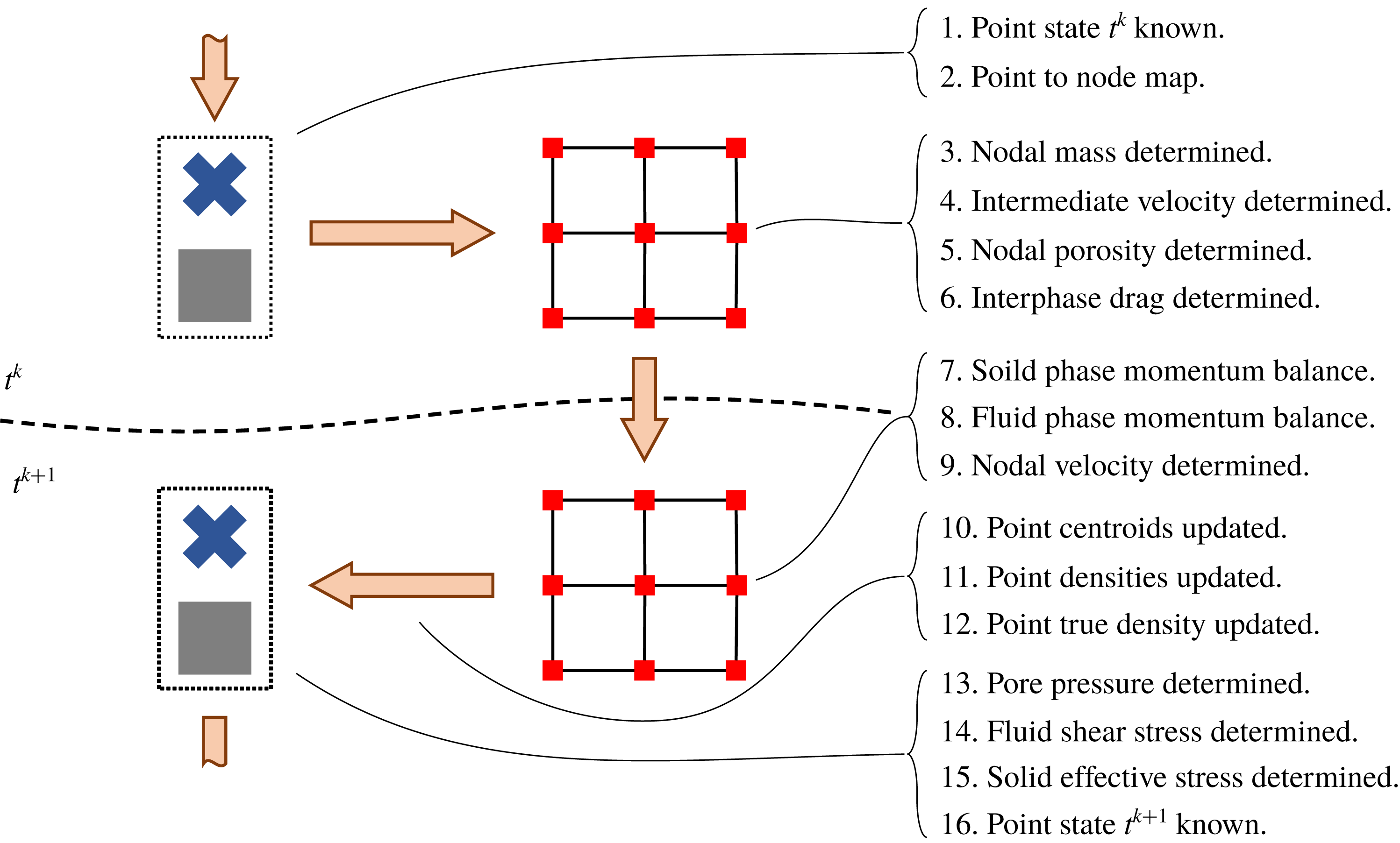
(i) The discrete material point states of the two phases are known at time $t^{k}$ .
(C 8) $$\begin{eqnarray}\displaystyle \left.\begin{array}{@{}c@{}}\text{solid phase: }\{\bar{\unicode[STIX]{x1D70C}}_{sp}^{k},\tilde{\unicode[STIX]{x1D748}}_{p}^{k},m_{sp},{\boldsymbol{x}_{s}}_{p}^{k},{\boldsymbol{v}_{s}}_{p}^{k}\}\\ \text{fluid phase: }\{\bar{\unicode[STIX]{x1D70C}}_{fp}^{k},\unicode[STIX]{x1D70C}_{fp}^{k},{\unicode[STIX]{x1D749}_{f}}_{p}^{k},p_{fp}^{k},m_{fp},{\boldsymbol{x}_{f}}_{p}^{k},{\boldsymbol{v}_{f}}_{p}^{k}\}.\end{array}\right\} & & \displaystyle\end{eqnarray}$$
(ii) The material point centroids, $\{{\boldsymbol{x}_{s}}_{p}^{k}\}$ and $\{{\boldsymbol{x}_{f}}_{p}^{k}\}$ are used to generate the mapping coefficients $\{{\mathcal{S}}_{sip}^{k}\}$ , $\{{\mathcal{S}}_{fip}^{k}\}$ , $\{\unicode[STIX]{x1D735}{\mathcal{S}}_{sip}^{k}\}$ and $\{\unicode[STIX]{x1D735}{\mathcal{S}}_{fip}^{k}\}$ .
(C 9) $$\begin{eqnarray}\left.\begin{array}{@{}c@{}}{\mathcal{S}}_{sip}^{k}={\mathcal{N}}_{i}({\boldsymbol{x}_{s}}_{p}^{k}),\quad \unicode[STIX]{x1D735}{\mathcal{S}}_{sip}^{k}=\text{grad}\,({\mathcal{N}}_{i}(\boldsymbol{x}))|_{{\boldsymbol{x}_{s}\,}_{p}^{k}}\\ {\mathcal{S}}_{fip}^{k}={\mathcal{N}}_{i}({\boldsymbol{x}_{f}}_{p}^{k}),\quad \unicode[STIX]{x1D735}{\mathcal{S}}_{fip}^{k}=\text{grad}\,({\mathcal{N}}_{i}(\boldsymbol{x}))|_{{\boldsymbol{x}_{f}\,}_{p}^{k}}.\end{array}\right\}\end{eqnarray}$$
(iii) The nodal mass coefficients, $\{m_{si}^{k}\}$ and $\{m_{fi}^{k}\}$ , are determined.
(C 10a,b ) $$\begin{eqnarray}m_{si}^{k}=\mathop{\sum }_{p=1}^{N_{s}}m_{sp}{\mathcal{S}}_{sip}^{k},\quad m_{fi}^{k}=\mathop{\sum }_{p=1}^{N_{f}}m_{fp}{\mathcal{S}}_{fip}^{k}.\end{eqnarray}$$
(iv) An intermediate nodal representation of the phase velocity fields, given by the coefficients $\{{\boldsymbol{v}_{s}}_{i}^{\ast }\}$ and $\{{\boldsymbol{v}_{f}}_{i}^{\ast }\}$ , is determined by approximating the material point velocity fields, given by the coefficients $\{{\boldsymbol{v}_{s}}_{p}^{k}\}$ and $\{{\boldsymbol{v}_{f}}_{p}^{k}\}$ .
(C 11a,b ) $$\begin{eqnarray}m_{i}^{k}{\boldsymbol{v}_{s}}_{i}^{\ast }=\mathop{\sum }_{p=1}^{N_{s}}m_{sp}{\boldsymbol{v}_{s}}_{p}^{k}{\mathcal{S}}_{sip}^{k},\quad m_{fi}^{k}{\boldsymbol{v}_{f}}_{i}^{\ast }=\mathop{\sum }_{p=1}^{N_{f}}m_{fp}{\boldsymbol{v}_{f}}_{p}^{k}{\mathcal{S}}_{sip}^{k}.\end{eqnarray}$$
(v) The nodal porosity coefficients, $\{n_{i}^{k}\}$ , are determined.
(C 12) $$\begin{eqnarray}n_{i}^{k}=1-\frac{m_{si}^{k}}{V_{i}\unicode[STIX]{x1D70C}_{s}}.\end{eqnarray}$$
(vi) The nodal approximation of the inter-phase drag, given by $\{\,{\boldsymbol{f}_{d}\,}_{i}^{\ast }\}$ , is determined.
(C 13) $$\begin{eqnarray}\displaystyle & \displaystyle {\boldsymbol{f}_{d}\,}_{i}^{\ast }=\frac{18n_{i}^{k}(1-n_{i}^{k})\unicode[STIX]{x1D702}_{0}}{d^{2}}~\hat{F}((1-n_{i}^{k}),Re_{i}^{\ast })({\boldsymbol{v}_{s}}_{i}^{\ast }-{\boldsymbol{v}_{f}}_{i}^{\ast })\mathop{\sum }_{p=1}^{N_{f}}v_{pf}^{k}{\mathcal{S}}_{fip}^{k} & \displaystyle\end{eqnarray}$$

(C 14) $$\begin{eqnarray}\displaystyle & \displaystyle Re_{i}^{\ast }=\frac{n_{i}^{k}\Vert {\boldsymbol{v}_{s}}_{i}^{\ast }-{\boldsymbol{v}_{f}}_{i}^{\ast }\Vert d}{\unicode[STIX]{x1D702}_{0}}. & \displaystyle\end{eqnarray}$$
(vii) The acceleration of the solid phase at time $t^{k+1}$ , given by $\{{\boldsymbol{a}_{s}}_{i}^{k+1}\}$ , is determined.
(C 15) $$\begin{eqnarray}\displaystyle m_{si}^{k}{\boldsymbol{a}_{s}}_{i}^{k+1} & = & \displaystyle m_{si}^{k}\boldsymbol{g}-{\boldsymbol{f}_{d}}_{i}^{k}-\mathop{\sum }_{p=1}^{N_{s}}(v_{sp}^{k}\tilde{\unicode[STIX]{x1D748}}_{p}^{k}\unicode[STIX]{x1D735}{\mathcal{S}}_{sip}^{k})+(1-n_{i}^{k})\mathop{\sum }_{p=1}^{N_{f}}(v_{fp}^{k}p_{fp}^{k}\unicode[STIX]{x1D735}{\mathcal{S}}_{sip}^{k})+{\boldsymbol{s}_{s}}_{i}^{k}\nonumber\\ \displaystyle & & \displaystyle \quad ({\boldsymbol{s}_{s}\,}_{i}^{k}\text{ is a boundary condition enforced on the }i\text{th node}).\quad\end{eqnarray}$$
(viii) The acceleration of the fluid phase at time $t^{k+1}$ , given by $\{{\boldsymbol{a}_{f}}_{i}^{k+1}\}$ , is determined.
(C 16) $$\begin{eqnarray}\displaystyle m_{fi}^{k}{\boldsymbol{a}_{f}}_{i}^{k+1} & = & \displaystyle m_{fi}^{k}\boldsymbol{g}+{\boldsymbol{f}_{d}\,}_{i}^{k}-\mathop{\sum }_{p=1}^{N_{f}}(v_{fp}^{k}{\unicode[STIX]{x1D749}_{f}}_{p}^{k}\unicode[STIX]{x1D735}{\mathcal{S}}_{fip}^{k})+n_{i}^{k}\mathop{\sum }_{p=1}^{N_{f}}(v_{fp}^{k}p_{fp}^{k}\unicode[STIX]{x1D735}{\mathcal{S}}_{sip}^{k})+{\boldsymbol{s}_{f}}_{i}^{k}\nonumber\\ \displaystyle & & \displaystyle \quad ({\boldsymbol{s}_{f}}_{i}^{k}\text{ is a boundary condition enforced on the }i\text{th node}).\quad\end{eqnarray}$$
(ix) The phase velocity fields at time $t^{k+1}$ , given by $\{{\boldsymbol{v}_{s}}_{i}^{k+1}\}$ and $\{{\boldsymbol{v}_{f}}_{i}^{k+1}\}$ , are determined explicitly according to,
(C 17a,b ) $$\begin{eqnarray}{\boldsymbol{v}_{s}}_{i}^{k+1}={\boldsymbol{v}_{s}}_{i}^{\ast }+\unicode[STIX]{x0394}t~{\boldsymbol{a}_{s}}_{i}^{k+1},\quad {\boldsymbol{v}_{f}}_{i}^{k+1}={\boldsymbol{v}_{f}}_{i}^{\ast }+\unicode[STIX]{x0394}t~{\boldsymbol{a}_{f}}_{i}^{k+1}.\end{eqnarray}$$
(x) The material point centroid positions and velocities are updated explicitly as in Brackbill & Ruppel (Reference Brackbill and Ruppel1986) and Brackbill, Kothe & Ruppel (Reference Brackbill, Kothe and Ruppel1988),
(C 18) $$\begin{eqnarray}\displaystyle \left.\begin{array}{@{}c@{}}\displaystyle {\boldsymbol{x}_{s}}_{p}^{k+1}={\boldsymbol{x}_{s}}_{p}^{k}+\unicode[STIX]{x0394}t~\mathop{\sum }_{i=1}^{[n]}{\boldsymbol{v}_{s}}_{i}^{k+1}{\mathcal{S}}_{sip}^{k}+({\unicode[STIX]{x1D739}_{s}}_{p}^{k}),\quad {\boldsymbol{v}_{s}}_{p}^{k+1}={\boldsymbol{v}_{s}}_{p}^{k}+\unicode[STIX]{x0394}t~\mathop{\sum }_{i=1}^{[n]}{\boldsymbol{a}_{s}}_{i}^{k+1}{\mathcal{S}}_{sip}^{k}\\ \displaystyle {\boldsymbol{x}_{f}}_{p}^{k+1}={\boldsymbol{x}_{f}}_{p}^{k}+\unicode[STIX]{x0394}t~\mathop{\sum }_{i=1}^{[n]}{\boldsymbol{v}_{f}}_{i}^{k+1}{\mathcal{S}}_{fip}^{k}+({\unicode[STIX]{x1D739}_{f}}_{p}^{k}),\quad {\boldsymbol{v}_{f}}_{p}^{k+1}={\boldsymbol{v}_{f}}_{p}^{k}+\unicode[STIX]{x0394}t~\mathop{\sum }_{i=1}^{[n]}{\boldsymbol{a}_{f}}_{i}^{k+1}{\mathcal{S}}_{fip}^{k},\end{array}\right\} & & \displaystyle \nonumber\\ \displaystyle & & \displaystyle\end{eqnarray}$$
where ${\unicode[STIX]{x1D739}_{s}}_{p}^{k+1}$ and ${\unicode[STIX]{x1D739}_{f}}_{p}^{k+1}$ are the $\unicode[STIX]{x1D6FF}$ position correction described in § C.4.5.
(xi) The material point densities at time $t^{k+1}$ , $\{\bar{\unicode[STIX]{x1D70C}}_{s}^{k+1}\}$ and $\{\bar{\unicode[STIX]{x1D70C}}_{s}^{k+1}\}$ , are updated.
(C 19) $$\begin{eqnarray}\left.\begin{array}{@{}c@{}}\displaystyle \bar{\unicode[STIX]{x1D70C}}_{sp}^{k+1}=\bar{\unicode[STIX]{x1D70C}}_{sp}^{k}\exp \left(-(\unicode[STIX]{x0394}t)\text{tr}\,\left(\mathop{\sum }_{i=1}^{[n]}{\boldsymbol{v}_{s}}_{i}^{k+1}\otimes \unicode[STIX]{x1D735}{\mathcal{S}}_{sip}^{k}\right)\right)\\ \displaystyle \bar{\unicode[STIX]{x1D70C}}_{fp}^{k+1}=\bar{\unicode[STIX]{x1D70C}}_{fp}^{k}\exp \left(-(\unicode[STIX]{x0394}t)\text{tr}\,\left(\mathop{\sum }_{i=1}^{[n]}{\boldsymbol{v}_{f}}_{i}^{k+1}\otimes \unicode[STIX]{x1D735}{\mathcal{S}}_{fip}^{k}\right)\right),\end{array}\right\}\end{eqnarray}$$
where $\otimes$ is the tensor product operator.
(xii) The fluid phase material point true densities, $\{\unicode[STIX]{x1D70C}_{fp}^{k+1}\}$ , are determined. (Note that for numerical stability, we do not require that $\{n_{p}^{k+1}\}$ , $\{\bar{\unicode[STIX]{x1D70C}}_{fp}^{k+1}\}$ , and $\{\unicode[STIX]{x1D70C}_{fp}^{k+1}\}$ be consistent.)
(C 20) $$\begin{eqnarray}\displaystyle & \displaystyle n_{p}^{k+1}=\mathop{\sum }_{i=1}^{[n]}n_{i}^{k}{\mathcal{S}}_{fip}^{k} & \displaystyle\end{eqnarray}$$

(C 21) $$\begin{eqnarray}\displaystyle & \displaystyle \unicode[STIX]{x1D70C}_{fp}^{k+1}=\unicode[STIX]{x1D70C}_{fp}^{k}\exp \left(-\left(\frac{\unicode[STIX]{x0394}t}{n_{p}^{k+1}}\right)\text{tr}\,\left(\mathop{\sum }_{i=1}^{[n]}[(1-n_{i}^{k}){\boldsymbol{v}_{s}}_{i}^{k+1}+n_{i}^{k}{\boldsymbol{v}_{f}}_{i}^{k+1}]\otimes \unicode[STIX]{x1D735}{\mathcal{S}}_{fip}^{k}\right)\right). & \displaystyle \nonumber\\ \displaystyle & & \displaystyle\end{eqnarray}$$
(xiii) The fluid phase material point pore pressure state is determined directly from the true fluid density.
(C 22) $$\begin{eqnarray}p_{fp}^{k+1}=\unicode[STIX]{x1D705}\ln \left(\frac{\unicode[STIX]{x1D70C}_{fp}^{k+1}}{\unicode[STIX]{x1D70C}_{0f}}\right).\end{eqnarray}$$
(xiv) The fluid phase material point shear stresses, $\{{\unicode[STIX]{x1D749}_{f}}_{p}^{k+1}\}$ , are determined directly from the fluid phase velocity gradient.
(C 23) $$\begin{eqnarray}\displaystyle \left.\begin{array}{@{}c@{}}\displaystyle {\unicode[STIX]{x1D749}_{f}}_{p}^{k+1}=2\unicode[STIX]{x1D702}_{0}\left(1+\frac{5}{2}(1-n_{p}^{k+1})\right){\unicode[STIX]{x1D63F}_{0f}}_{p}^{k+1}\\ \displaystyle {\unicode[STIX]{x1D63F}_{f}}_{p}^{k+1}=\text{sym}\left(\mathop{\sum }_{i=1}^{[n]}{\boldsymbol{v}_{f}}_{i}^{k+1}\otimes \unicode[STIX]{x1D735}{\mathcal{S}}_{fip}^{k}\right).\end{array}\right\} & & \displaystyle\end{eqnarray}$$
(xv) The solid phase material point effective stresses, $\{\tilde{\unicode[STIX]{x1D748}}_{p}^{k+1}\}$ , are determined with a semi-implicit method described in § C.3.
(C 24) $$\begin{eqnarray}\displaystyle \tilde{\unicode[STIX]{x1D748}}_{p}^{k+1} & = & \displaystyle \tilde{\unicode[STIX]{x1D748}}_{p}^{k}+\unicode[STIX]{x0394}t\left[\right.\!2G({\unicode[STIX]{x1D63F}_{0s}}_{p}^{k+1}-(\tilde{\unicode[STIX]{x1D63F}}_{0}^{p})_{p}^{k+1})\nonumber\\ \displaystyle & & \displaystyle +\,K\text{tr}\,({\unicode[STIX]{x1D63F}_{s}}_{p}^{k+1}-(\tilde{\unicode[STIX]{x1D63F}^{\,p}})_{p}^{k+1})\mathbf{1}+{\unicode[STIX]{x1D652}_{s}}_{p}^{k+1}\tilde{\unicode[STIX]{x1D748}}_{p}^{k}-\tilde{\unicode[STIX]{x1D748}}_{p}^{k}{\unicode[STIX]{x1D652}_{s}}_{p}^{k+1}\!\left.\right].\end{eqnarray}$$
(xvi) The discrete material point states of the two phases are known for time $t^{k+1}$ ,
(C 25) $$\begin{eqnarray}\displaystyle \left.\begin{array}{@{}l@{}}\text{solid phase: }\{\bar{\unicode[STIX]{x1D70C}}_{sp}^{k+1},\tilde{\unicode[STIX]{x1D748}}_{p}^{k+1},m_{sp},{\boldsymbol{x}_{s}}_{p}^{k+1},{\boldsymbol{v}_{s}}_{p}^{k+1}\}\\ \text{fluid phase: }\{\bar{\unicode[STIX]{x1D70C}}_{fp}^{k+1},\unicode[STIX]{x1D70C}_{fp}^{k+1},{\unicode[STIX]{x1D749}_{f}}_{p}^{k+1},p_{fp}^{k+1},m_{fp},{\boldsymbol{x}_{f}}_{p}^{k+1},{\boldsymbol{v}_{f}}_{p}^{k+1}\}\end{array}\right\} & & \displaystyle\end{eqnarray}$$
and the procedure is repeated for the $k+1$ time step.

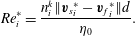
C.3 Semi-implicit effective stress algorithm

The solid phase material point effective stress is updated at each time step with the semi-implicit time integration scheme described in this section. Given the material point stress states at time $t^{k}$ , $\{\tilde{\unicode[STIX]{x1D748}}_{p}^{k}\}$ , and the total material point flow rates at time $t^{k+1}$ ,

(C 26a-c )

$$\begin{eqnarray}{\unicode[STIX]{x1D63F}_{s}}_{p}^{k+1}=\text{sym}({\unicode[STIX]{x1D647}_{s}}_{p}^{k+1}),\quad {\unicode[STIX]{x1D652}_{s}}_{p}^{k+1}=\text{skw}({\unicode[STIX]{x1D647}_{s}}_{p}^{k+1}),\quad {\unicode[STIX]{x1D647}_{s}}_{p}^{k+1}=\mathop{\sum }_{i=1}^{[n]}{\boldsymbol{v}_{f}}_{i}^{k+1}\otimes \unicode[STIX]{x1D735}{\mathcal{S}}_{fip}^{k}\end{eqnarray}$$

we solve for the plastic flow rates $\{(\tilde{\unicode[STIX]{x1D63F}^{\,p}})_{p}^{k+1}\}$ given by,

(C 27)

$$\begin{eqnarray}(\tilde{\unicode[STIX]{x1D63F}^{\,p}})_{p}^{k+1}=\frac{(\dot{\bar{\unicode[STIX]{x1D6FE}}}^{p})_{p}^{k+1}}{\sqrt{2}}\frac{{\tilde{\unicode[STIX]{x1D748}}_{0}\,}_{p}^{k+1}}{\Vert {\tilde{\unicode[STIX]{x1D748}}_{0}\,}_{p}^{k+1}\Vert }+\frac{1}{3}\big(\unicode[STIX]{x1D6FD}(\dot{\bar{\unicode[STIX]{x1D6FE}}}^{p})_{p}^{k+1}+(\dot{\unicode[STIX]{x1D709}}_{1})_{p}^{k+1}+(\dot{\unicode[STIX]{x1D709}}_{2})_{p}^{k+1}\big)\mathbf{1}\end{eqnarray}$$

such that (with $(\dot{\bar{\unicode[STIX]{x1D6FE}}}^{p})_{p}^{k+1}$ , $(\dot{\unicode[STIX]{x1D709}}_{1})_{p}^{k+1}$ , and $(\dot{\unicode[STIX]{x1D709}}_{2})_{p}^{k+1}$ determined for each material point) the material point stress state at time $t^{k+1}$ is given by (C 24).

C.3.1 Definition of trial stress

The update from (C 24) can be separated into a trial step,

(C 28)

$$\begin{eqnarray}\tilde{\unicode[STIX]{x1D748}}_{p}^{tr}=\tilde{\unicode[STIX]{x1D748}}_{p}^{k}+\unicode[STIX]{x0394}t[2G{\unicode[STIX]{x1D63F}_{0s}}_{p}^{k+1}+K\text{tr}\,({\unicode[STIX]{x1D63F}_{s}}_{p}^{k+1})\mathbf{1}+{\unicode[STIX]{x1D652}_{s}}_{p}^{k+1}\tilde{\unicode[STIX]{x1D748}}_{p}^{k}-\tilde{\unicode[STIX]{x1D748}}_{p}^{k}{\unicode[STIX]{x1D652}_{s}}_{p}^{k+1}]\end{eqnarray}$$

and a plastic step,

(C 29)

$$\begin{eqnarray}\tilde{\unicode[STIX]{x1D748}}_{p}^{k+1}=\tilde{\unicode[STIX]{x1D748}}_{p}^{tr}-\unicode[STIX]{x0394}t[2G(\tilde{\unicode[STIX]{x1D63F}}_{0}^{p})_{p}^{k+1}+K\text{tr}\,((\tilde{\unicode[STIX]{x1D63F}^{\,p}})_{p}^{k+1})\mathbf{1}],\end{eqnarray}$$

where $\tilde{\unicode[STIX]{x1D748}}_{p}^{tr}$ is a trial stress found between times $t^{k}$ and $t^{k+1}$ . Since the trial stress given in (C 28) is an explicit function of the strain rates in (C 29), we use it as the starting point of our implicit algorithm for solving (C 29).

C.3.2 Simplification to scalar relation

The expression in (C 29) is separable into a deviatoric part and isotropic part,

(C 30a,b )

$$\begin{eqnarray}\tilde{\unicode[STIX]{x1D748}}_{0_{p}^{k+1}}=\tilde{\unicode[STIX]{x1D748}}_{0_{p}}^{\,\;tr}-2G\unicode[STIX]{x0394}t(\tilde{\unicode[STIX]{x1D63F}}_{0}^{p})_{p}^{k+1},\quad \text{tr}\,(\tilde{\unicode[STIX]{x1D748}})_{p}^{k+1}=\text{tr}\,(\tilde{\unicode[STIX]{x1D748}})_{p}^{tr}-3K\unicode[STIX]{x0394}\text{tr}\,((\tilde{\unicode[STIX]{x1D63F}^{\,p}})_{p}^{k+1}).\end{eqnarray}$$

The following scalar stress measures reduce the implicit tensor relations above to a set of implicit scalar relations (which are much simpler to solve numerically),

(C 31a-d )

$$\begin{eqnarray}\bar{\unicode[STIX]{x1D70F}}_{p}^{tr}=\frac{\Vert \tilde{\unicode[STIX]{x1D748}}_{0_{p}}^{\,\;tr}\Vert }{\sqrt{2}},\quad \bar{\unicode[STIX]{x1D70F}}_{p}^{k+1}=\frac{\Vert \tilde{\unicode[STIX]{x1D748}}_{p}^{k+1}\Vert }{\sqrt{2}},\quad \tilde{p}_{p}^{tr}=-\frac{1}{3}\text{tr}\,(\tilde{\unicode[STIX]{x1D748}}_{0_{p}}^{\,\;tr}),\quad \tilde{p}_{p}^{k+1}=-\frac{1}{3}\text{tr}\,(\tilde{\unicode[STIX]{x1D748}}_{p}^{k+1})\end{eqnarray}$$

and therefore (C 29) becomes,

(C 32)

$$\begin{eqnarray}\displaystyle & \displaystyle \bar{\unicode[STIX]{x1D70F}}_{p}^{k+1}=\bar{\unicode[STIX]{x1D70F}}_{p}^{tr}-G\unicode[STIX]{x0394}t~(\dot{\bar{\unicode[STIX]{x1D6FE}}}^{p})_{p}^{k+1} & \displaystyle\end{eqnarray}$$

(C 33)

$$\begin{eqnarray}\displaystyle & \displaystyle \tilde{p}_{p}^{k+1}=\tilde{p}_{p}^{tr}+K\unicode[STIX]{x0394}t(\unicode[STIX]{x1D6FD}(\dot{\bar{\unicode[STIX]{x1D6FE}}}^{p})_{p}^{k+1}+(\dot{\unicode[STIX]{x1D709}}_{1})_{p}^{k+1}+(\dot{\unicode[STIX]{x1D709}}_{2})_{p}^{k+1}). & \displaystyle\end{eqnarray}$$

By solving the system of equations in (C 32) and (C 33) subject to the following discrete yield conditions,

(C 34)

$$\begin{eqnarray}\left.\begin{array}{@{}l@{}}(f_{1})_{p}^{k+1}=\bar{\unicode[STIX]{x1D70F}}_{p}^{k+1}-\max ((\unicode[STIX]{x1D707}_{p}+\unicode[STIX]{x1D6FD})\tilde{p}_{p}^{k+1},0)\\ (f_{1})_{p}^{k+1}\leqslant 0,\quad (\dot{\bar{\unicode[STIX]{x1D6FE}}}^{p})_{p}^{k+1}\geqslant 0,\quad (f_{1})_{p}^{k+1}(\dot{\bar{\unicode[STIX]{x1D6FE}}}^{p})_{p}^{k+1}=0\\ (f_{2})_{p}^{k+1}=-\tilde{p}_{p}^{k+1}\\ (f_{2})_{p}^{k+1}\leqslant 0,\quad (\dot{\unicode[STIX]{x1D709}}_{1})_{p}^{k+1}\geqslant 0,\quad (f_{2})_{p}^{k+1}(\dot{\unicode[STIX]{x1D709}}_{1})_{p}^{k+1}=0\\ (f_{3})_{p}^{k+1}=g(\unicode[STIX]{x1D719})\tilde{p}_{p}^{k+1}-(a\unicode[STIX]{x1D719})^{2}[((\dot{\bar{\unicode[STIX]{x1D6FE}}}^{p})_{p}^{k+1}-K_{4}(\dot{\unicode[STIX]{x1D709}}_{2})_{p}^{k+1})^{2}d^{2}\unicode[STIX]{x1D70C}_{s}+2\unicode[STIX]{x1D702}_{0}((\dot{\bar{\unicode[STIX]{x1D6FE}}}^{p})_{p}^{k+1}-K_{4}(\dot{\unicode[STIX]{x1D709}}_{2})_{p}^{k+1})]\\ (f_{3})_{p}^{k+1}\leqslant 0,\quad (\dot{\unicode[STIX]{x1D709}}_{2})_{p}^{k+1}\leqslant 0,\quad (f_{3})_{p}^{k+1}(\dot{\unicode[STIX]{x1D709}}_{2})_{p}^{k+1}=0\end{array}\right\}\end{eqnarray}$$

we arrive at the final effective granular stresses at time $t^{k+1}$ ,

(C 35)

$$\begin{eqnarray}\tilde{\unicode[STIX]{x1D748}}_{p}^{k+1}=\frac{\bar{\unicode[STIX]{x1D70F}}_{p}^{k+1}}{\bar{\unicode[STIX]{x1D70F}}_{p}^{tr}}\tilde{\unicode[STIX]{x1D748}}_{0_{p}}^{\,\;tr}-\tilde{p}_{p}^{k+1}\mathbf{1}.\end{eqnarray}$$

C.3.3 Complete algorithm for stress update

To solve the system of equations from § C.3.2, we use the procedure described in algorithm 1 to successively project the trial stress state defined by $\{\tilde{p}_{p}^{tr}\}$ and $\{\bar{\unicode[STIX]{x1D70F}}_{p}^{tr}\}$ to the yield surfaces given in (C 34). As shown in figure 23, once an admissible stress update is found, the algorithm exits and proceeds to the next time step. In our implementation of this procedure, we choose to use a simple Newton iteration scheme to solve for each of the projections.

Figure 23.

The basic solid phase effective stress update proceeds as follows. (a) A trial step is taken from the stress state at time $t^{k}$ assuming that all flow is elastic. (b) The method described in algorithm 1 is used to determine how to project the trial stress to an admissible stress state. (c) The final stress state is updated from the trial stress state.

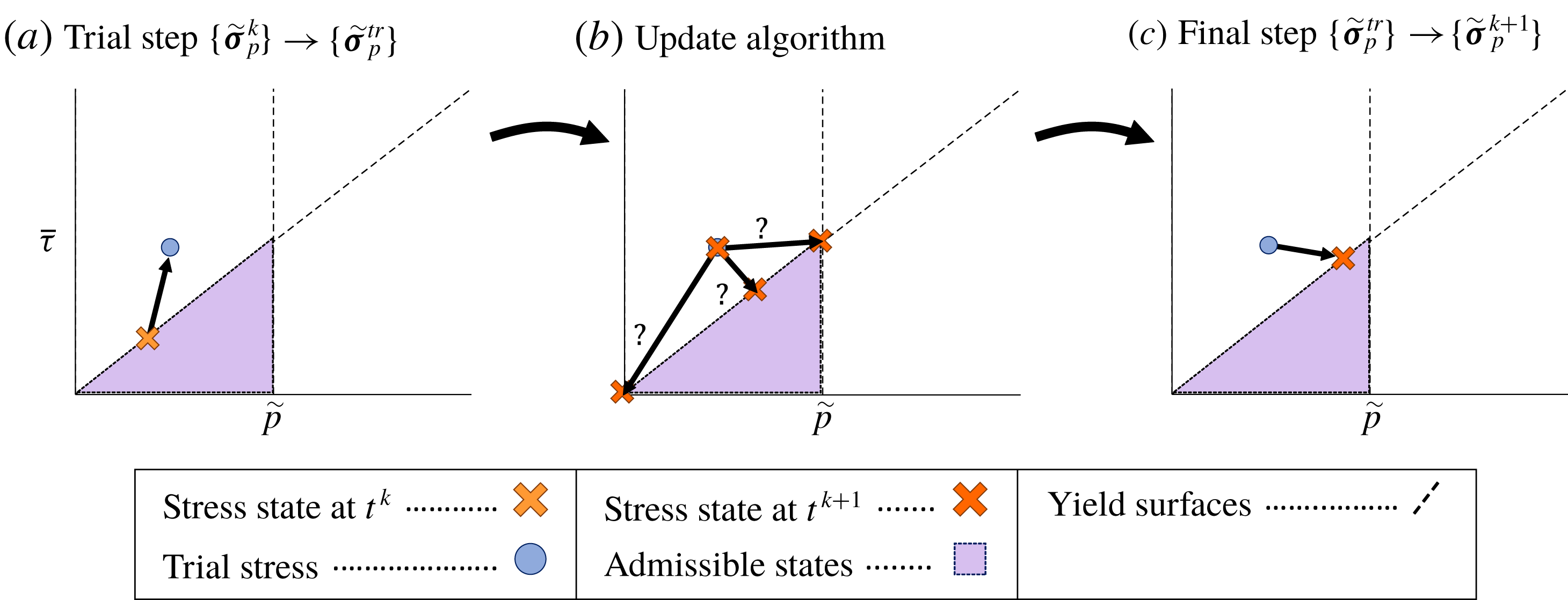
C.4 Specific notes about implementation

In this section we briefly discuss the implementation of the boundary conditions, contact forces, partial saturation and what we call the $\unicode[STIX]{x1D6FF}$ position correction.

C.4.1 Kinematic boundary conditions

The kinematic boundary condition used in this work is inherited from that used by Dunatunga & Kamrin (Reference Dunatunga and Kamrin2015). In this method, the boundary force vectors, ${\boldsymbol{s}_{s}}_{i}^{k}$ and ${\boldsymbol{s}_{f}}_{i}^{k}$ , on the boundary nodes are determined such that some prescribed velocity is achieved at the end of the explicit time step.

C.4.2 Mixed boundary conditions

In some simulations, we implement a frictional boundary condition on the solid phase. For these simulations, only the component of ${\boldsymbol{v}_{s}}_{p}^{k+1}$ normal to the boundary is prescribed (and therefore, the normal component of ${\boldsymbol{s}_{s}}_{i}^{k}$ is also determined). We then let the tangential force component be given by either a no-slip condition or,

(C 36)

$$\begin{eqnarray}{\boldsymbol{s}_{s}}_{i}^{k}-({\boldsymbol{s}_{s}}_{i}^{k}\boldsymbol{\cdot }\boldsymbol{n}_{b_{i}})\boldsymbol{n}_{b_{i}}=-\unicode[STIX]{x1D707}_{1}\left\Vert \mathop{\sum }_{p=1}^{N_{s}}(v_{sp}\tilde{p}_{p}^{k}\unicode[STIX]{x1D735}{\mathcal{S}}_{sip})\right\Vert \frac{{\boldsymbol{v}_{s}}_{i}^{\ast }-({\boldsymbol{v}_{s}}_{i}^{\ast }\boldsymbol{\cdot }\boldsymbol{n}_{b_{i}})\boldsymbol{n}_{b_{i}}}{\Vert {\boldsymbol{v}_{s}}_{i}^{\ast }-({\boldsymbol{v}_{s}}_{i}^{\ast }\boldsymbol{\cdot }\boldsymbol{n}_{b_{i}})\boldsymbol{n}_{b_{i}}\Vert }\end{eqnarray}$$

whichever is smaller, where $\boldsymbol{n}_{b_{i}}$ is the boundary normal at the $i$ th node.

C.4.3 Contact algorithm

In some of the qualitative results presented in this work, we implement the contact algorithm from Huang et al. (Reference Huang, Zhang, Ma and Huang2011). This algorithm calculates an explicit inter-body force (when a third material body is introduced) which enforces a frictional, non-penetrating contact between the third body and each of the two phases presented in this work.

C.4.4 Partial immersion

In the parts of the solid body where there is no fluid, we say that the viscosity, $\unicode[STIX]{x1D702}_{0}$ , is zero. Numerically we accomplish this by constructing a nodal viscosity field at each time step given by the coefficients $\{\unicode[STIX]{x1D702}_{0i}^{k}\}$ . We then let the value of $\unicode[STIX]{x1D702}_{0}$ in § C.2 be determined on each solid phase material point by, $\{\unicode[STIX]{x1D702}_{0p}^{k}\}$ where,

(C 37a,b )

$$\begin{eqnarray}\unicode[STIX]{x1D702}_{0i}^{k}=\left\{\begin{array}{@{}ll@{}}\unicode[STIX]{x1D702}_{0}\quad & \text{if }m_{fi}^{k}>0\\ 0\quad & \text{if }m_{fi}^{k}=0\end{array}\right.\quad \forall i\in [1,[n]],\quad \unicode[STIX]{x1D702}_{0p}^{k}=\mathop{\sum }_{i=1}^{[n]}\unicode[STIX]{x1D702}_{0i}^{k}{\mathcal{S}}_{sip}\quad \forall p\in [1,N_{s}].\end{eqnarray}$$

C.4.5 Dynamic quadrature error reduction

Particle methods for simulating fluid flows have an inherent problem with (among other things) point clumping (see recent work by Koh, Gao & Luo (Reference Koh, Gao and Luo2012) and Maljaars (Reference Maljaars2016)). There are many physically admissible flows, such as those with stagnation points, which will result in material point tracers gathering together. By choosing the material point centroids as the quadrature points for our integral approximations, this clumping leads to significant quadrature error. In some fluid simulations, we see extremely spurious flows develop, which we attribute to this quadrature error.

To address this issue, we have developed a novel approach which ‘nudges’ material point centroids as the material flows. This nudge is the ${\unicode[STIX]{x1D739}_{s}}_{p}^{k}$ and ${\unicode[STIX]{x1D739}_{f}}_{p}^{k}$ from (C 18). The method we introduce relies on the nodal weight measure from (C 5) (which is known a priori). Since our material point characteristic functions are partitions of unity within the body (by C 1), we have,

(C 38)

$$\begin{eqnarray}V_{i}=\mathop{\sum }_{p=1}^{N_{s}}\int _{\unicode[STIX]{x1D6FA}}{\mathcal{N}}_{i}(\boldsymbol{x})U_{\unicode[STIX]{x1D6FC}p}(\boldsymbol{x})\,\text{d}v\quad \text{if}~({\mathcal{N}}_{i}(\boldsymbol{x})=0~\text{for}~\boldsymbol{x}\notin {\mathcal{B}}_{\unicode[STIX]{x1D6FC}}^{t}),\end{eqnarray}$$

where $\unicode[STIX]{x1D6FC}$ is a more general notation for either $s$ or $f$ .

We determine how much quadrature error has accumulated by using the material point weights and centroids as quadrature points for the above integral and measure the relative overshoot error, $e_{si}$ and $e_{fi}$ , as follows,

(C 39a,b )

$$\begin{eqnarray}v_{\unicode[STIX]{x1D6FC}i}\equiv \mathop{\sum }_{p=1}^{N_{\unicode[STIX]{x1D6FC}}}v_{\unicode[STIX]{x1D6FC}p}{\mathcal{N}}_{i}(\boldsymbol{x}_{\unicode[STIX]{x1D6FC}_{p}}),\quad e_{\unicode[STIX]{x1D6FC}i}=\max \left(0,\frac{v_{\unicode[STIX]{x1D6FC}i}-V_{i}}{V_{i}}\right).\end{eqnarray}$$

We have attempted several methods of reducing this error (which will be explored in a future work); however the method used in this work is a strain-rate-dependent position correction given as follows,

(C 40)

$$\begin{eqnarray}{\unicode[STIX]{x1D739}_{\unicode[STIX]{x1D6FC}}}_{p}^{k}=-\unicode[STIX]{x1D706}\unicode[STIX]{x0394}t(\unicode[STIX]{x0394}x)^{2}\Vert {\boldsymbol{L}_{\unicode[STIX]{x1D6FC}0}}_{p}^{k+1}\Vert \mathop{\sum }_{i=1}^{[n]}e_{\unicode[STIX]{x1D6FC}i}\unicode[STIX]{x1D735}{\mathcal{S}}_{\unicode[STIX]{x1D6FC}ip},\end{eqnarray}$$

with $\unicode[STIX]{x0394}x$ the grid spacing of the Cartesian grid and $\unicode[STIX]{x1D706}$ an arbitrary scale factor.

References

Abe, K., Soga, K. & Bandara, S. 2013 Material point method for coupled hydromechanical problems. J. Geotech. Geoenviron. Engng 140 (3), 04013033.Google Scholar

Allen, B. & Kudrolli, A. 2017 Depth resolved granular transport driven by shearing fluid flow. Phys. Rev. Fluids 2 (2), 024304.Google Scholar

Amarsid, L., Delenne, J. Y., Mutabaruka, P., Monerie, Y., Perales, F. & Radjai, F. 2017 Viscoinertial regime of immersed granular flows. Phys. Rev. E 96, 012901.Google Scholar

Anand, L. & Su, C. 2005 A theory for amorphous viscoplastic materials undergoing finite deformations, with applications to metallic glasses. J. Mech. Phys. Solids 53 (6), 1362–1396.Google Scholar

Bandara, S. & Soga, K. 2015 Coupling of soil deformation and pore fluid flow using material point method. Comput. Geotech. 63, 199–214.Google Scholar

Bardenhagen, S. G. & Kober, E. M. 2004 The generalized interpolation material point method. Comput. Model. Engng Sci. 5 (6), 477–496.Google Scholar

Beetstra, R., van der Hoef, M. A. & Kuipers, J. A. M. 2007 Drag force of intermediate Reynolds number flow past mono- and bidisperse arrays of spheres. AIChE J. 53 (2), 489–501.Google Scholar

Boyer, F., Gauzelli, E. & Pouliquen, O. 2011 Unifying suspension and granular rheology. Phys. Rev. Lett. 107 (18), 188301.Google Scholar

Brackbill, J. U. & Ruppel, H. M. 1986 Flip: a method for adaptively zoned, particle-in-cell calculations of fluid flows in two dimensions. J. Comput. Phys. 65 (2), 314–343.Google Scholar

Brackbill, J. U., Kothe, D. B. & Ruppel, H. M. 1988 Flip: a low-dissipation, particle-in-cell method for fluid flow. Comput. Phys. Commun. 48 (1), 25–38.Google Scholar

Carman, P. C. 1937 Fluid flow through granular beds. Trans. Inst. Chem. Engrs 15, 150–166.Google Scholar

Cassar, C., Nicolas, M. & Pouliquen, O. 2005 Submarine granular flows down inclined planes. Phys. Fluids 17 (10), 103301.Google Scholar

Ceccato, F., Beuth, L., Vermeer, P. A. & Simonini, P. 2016 Two-phase material point method applied to the study of cone penetration. Comput. Geotech. 80, 440–452.Google Scholar

Ceccato, F. & Simonini, P. 2016 Granular flow impact forces on protection structures: Mpm numerical simulations with different constitutive models. Proc. Engng 158, 164–169.Google Scholar

Chang, C. & Powell, R. L. 1993 Dynamic simulation of bimodal suspensions of hydrodynamically interacting spherical particles. J. Fluid Mech. 253, 1–25.Google Scholar

Chang, C. & Powell, R. L. 1994 Effect of particle size distributions on the rheology of concentrated bimodal suspensions. J. Rheol. 38 (1), 85–98.Google Scholar

Chong, J. S., Christiansen, E. B. & Baer, A. D. 1971 Rheology of concentrated suspensions. J. Appl. Polym. Sci. 15 (8), 2007–2021.Google Scholar

Clift, R., Grace, J. R. & Weber, M. E. 2005 Bubbles, Drops, and Particles. Courier Corporation.Google Scholar

Cook, B. K., Noble, D. R. & Williams, J. R. 2004 A direct simulation method for particle-fluid systems. Engng Comput. 21 (2/3/4), 151–168.Google Scholar

Coussy, O. 2004 Poromechanics. Wiley.Google Scholar

Da Cruz, F., Emam, S., Prochnow, M., Roux, J.-N. & Chevoir, F. 2005 Rheophysics of dense granular materials: discrete simulation of plane shear flows. Phys. Rev. E 72 (2), 021309.Google Scholar

Drumheller, D. S. 2000 On theories for reacting immiscible mixtures. Intl J. Engng Sci. 38, 347–382.Google Scholar

Dunatunga, S. & Kamrin, K. 2015 Continuum modelling and simulation of granular flows through their many phases. J. Fluid Mech. 779, 483–513.Google Scholar

Dupuit, J. É. J. 1863 Études théoriques et pratiques sur le mouvement des eaux dans les canaux découverts et à travers les terrains perméables: avec des considérations relatives au régime des grandes eaux, au débouché à leur donner, et à la marche des alluvions dans les rivières à fond mobile. Dunod.Google Scholar

Einstein, A. 1906 Calculation of the viscosity-coefficient of a liquid in which a large number of small spheres are suspended in irregular distribution. Ann. Phys. Leipzig 19, 286–306.Google Scholar

Fern, E. J. & Soga, K. 2016 The role of constitutive models in mpm simulations of granular column collapses. Acta Geotech. 11 (3), 659–678.Google Scholar

Gurtin, M. E., Fried, E. & Anand, L. 2010 The Mechanics and Thermodynamics of Continua. Cambridge University Press.Google Scholar

Henann, D. L. & Kamrin, K. 2013 A predictive, size-dependent continuum model for dense granular flows. Proc. Natl Acad. Sci. 110 (17), 6730–6735.Google Scholar

van der Hoef, M. A., Beetstra, R. & Kuipers, J. A. M. 2005 Lattice-Boltzmann simulations of low-Reynolds-number flow past mono- and bidisperse arrays of spheres: results for the permeability and drag force. J. Fluid Mech. 528, 233–254.Google Scholar

Houssais, M., Ortiz, C. P., Durian, D. J. & Jerolmack, D. J. 2015 Onset of sediment transport is a continuous transition driven by fluid shear and granular creep. Nat. Commun. 6, 6527.Google Scholar

Huang, P., Zhang, X., Ma, S. & Huang, X. 2011 Contact algorithms for the material point method in impact and penetration simulation. Intl J. Numer. Meth. Engng 85 (4), 498–517.Google Scholar

Jackson, R. 2000 The Dynamics of Fluidized Particles. Cambridge University Press.Google Scholar

Jop, P., Forterre, Y. & Pouliquen, O. 2006 A constitutive law for dense granular flows. Nature 441 (7094).Google Scholar

Kamrin, K. & Henann, D. L. 2015 Nonlocal modeling of granular flows down inclines. Soft Matt. 11 (1), 179–185.Google Scholar

Kamrin, K. & Koval, G. 2012 Nonlocal constitutive relation for steady granular flow. Phys. Rev. Lett. 108 (17), 178301.Google Scholar

Klika, V. 2014 A guide through available mixture theories for applications. Critical Rev. Solid State Mater. Sci. 39 (2), 154–174.Google Scholar

Koh, C. G., Gao, M. & Luo, C. 2012 A new particle method for simulation of incompressible free surface flow problems. Intl J. Numer. Methods Engng 89 (12), 1582–1604.Google Scholar

Maljaars, J. M.2016 A hybrid particle-mesh method for simulating free surface flows. Delft University of Technology.Google Scholar

Mast, C. M., Mackenzie-Helnwein, P., Arduino, P., Miller, G. R. & Shin, W. 2012 Mitigating kinematic locking in the material point method. J. Comput. Phys. 231 (16), 5351–5373.Google Scholar

Pailha, M. & Pouliquen, O. 2009 A two-phase flow description of the initiation of underwater granular avalanches. J. Fluid Mech. 633, 115–135.Google Scholar

Poslinski, A. J., Ryan, M. E., Gupta, R. K., Seshadri, S. G. & Frechette, F. J. 1988 Rheological behavior of filled polymeric systems ii. The effect of a bimodal size distribution of particulates. J. Rheol. 32 (8), 751–771.Google Scholar

Rondon, L., Pouliquen, O. & Aussillous, P. 2011 Granular collapse in a fluid: role of the initial volume fraction. Phys. Fluids 23 (7), 073301.Google Scholar

Roux, S. & Radjai, F. 1998 Texture-dependent rigid-plastic behavior. In Physics of Dry Granular Media (ed. Herrmann, H. J., Hovi, J. P. & Luding, S.), pp. 229–236. Springer.Google Scholar

Roux, S. & Radjai, F. 2001 Statistical approach to the mechanical behavior of granular media. In Mechanics for a New Mellennium (ed. Aref, H. & Phillips, J. W.), pp. 181–196. Kluwer.Google Scholar

Rudnicki, J. W. & Rice, J. R. 1975 Conditions for the localization of deformation in pressure-sensitive dilatant materials. J. Mech. Phys. Solids 23 (6), 371–394.Google Scholar

Shapiro, A. P. & Probstein, R. F. 1992 Random packings of spheres and fluidity limits of monodisperse and bidisperse suspensions. Phys. Rev. Lett. 68 (9), 1422–1425.Google Scholar

Soga, K., Alonso, E., Yerro, A., Kumar, K. & Bandara, S. 2015 Trends in large-deformation analysis of landslide mass movements with particular emphasis on the material point method. Geotechnique 66 (3), 248–273.Google Scholar

Steffen, M., Kirby, R. M. & Berzins, M. 2008 Analysis and reduction of quadrature errors in the material point method (mpm). Intl J. Numer. Meth. Engng 76 (6), 922–948.Google Scholar

Stickel, J. J. & Powell, R. L. 2005 Fluid mechanics and rheology of dense suspensions. Annu. Rev. Fluid Mech. 37, 129–149.Google Scholar

Storms, R. F., Ramarao, B. V. & Weiland, R. H. 1990 Low shear rate viscosity of bimodally dispersed suspensions. Powder Technol. 63 (3), 247–259.Google Scholar

Sulsky, D., Chen, Z. & Schreyer, H. L. 1994 A particle method for history-dependent materials. Comput. Meth. Appl. Mech. Engng 118 (1–2), 179–196.Google Scholar

Truesdell, C. & Noll, W. 1965 The Non-Linear Field Theories of Mechanics. Springer.Google Scholar

Turian, R. M. & Yuan, T.-F. 1977 Flow of slurries in pipelines. AIChE J. 23 (3), 232–243.Google Scholar

Wilmanski, K. 2008 Continuum Thermodynamics – Part 1: Foundations. World Scientific.Google Scholar

Zhao, Y. & Davis, R. H. 2002 Interaction of two touching spheres in a viscous fluid. Chem. Engng Sci. 57 (11), 1997–2006.Google Scholar

Figure 1.Pictorial description of the representative volume $\unicode[STIX]{x1D6FA}$, the decomposition of the domain into fluid and solid volumes, and the homogenization of the two phases.

Figure 2.(a) Pictorial definition of the reference bodies, ${\mathcal{B}}^{s}$ and ${\mathcal{B}}^{f}$, and deformed bodies, ${\mathcal{B}}_{t}^{s}$ and ${\mathcal{B}}_{t}^{f}$. (b) Parts in the deformed body are always fully saturated with porosity $n>0$. In the limit of a fluid-only volume, the porosity $n=1$. In the limit of a solid-only volume, we do not let the porosity $n$ go to zero, instead we let the fluid viscosity, bulk modulus and true density go to zero which effectively removes the fluid by making it stress and density free.

Figure 3.The three regimes over which the inter-phase drag $\boldsymbol{f}_{d}$ must be defined. The normalized average drag force $\langle F\rangle$ is taken from van der Hoef, Beetstra & Kuipers (2005) to be the average force on a single grain for a given packing fraction $\unicode[STIX]{x1D719}$ at a given flow rate.

Table 1.Summary of thermodynamic rules for constitutive laws derived in appendix A.

Figure 4.(a) In shear, the granular phase will obey critical state behaviour. This phenomenon is called Reynolds’ dilation and is captured by the rate of plastic dilation, $\unicode[STIX]{x1D6FD}\dot{\bar{\unicode[STIX]{x1D6FE}}}^{p}$. (b) In expansion, the granular phase will come apart freely. This phenomenon is stress free and is captured by the rate of plastic expansion, $\dot{\unicode[STIX]{x1D709}}_{1}$. (c) In compaction, granular collisions will result in a macroscopic pressure. This phenomenon is governed by the rate of plastic compaction, $-\dot{\unicode[STIX]{x1D709}}_{2}$.

Table 2.Parameters for model fit to data in figure 5.

Figure 5.Plot of the ratio between the shear stress and effective granular pressure ($\unicode[STIX]{x1D707}$) against the inertial number $I_{v}$. Data collected by Boyer et al. (2011) are shown as the shaded blue circles. The $\unicode[STIX]{x1D707}(I_{v})$ rheology from that work is represented by the dotted line. The combined response of the mixture model presented in this work (see (3.9)) is represented by the solid line.

Figure 6.Plot of various models for effective viscosity $\unicode[STIX]{x1D702}_{r}$ versus the relative packing fraction $\unicode[STIX]{x1D719}/\unicode[STIX]{x1D719}_{m}$. The model given in this work by (3.11) is shown by the solid line. The red diamonds represent the experimental results reported in Chang & Powell (1994) (from Chong, Christiansen & Baer (1971), Poslinski et al. (1988), Storms, Ramarao & Weiland (1990), Shapiro & Probstein (1992), Chang & Powell (1993) and Chang & Powell (1994)). The blue circles represent the experimental results reported in Boyer et al. (2011).

Table 3.Summary of governing equations derived in § 2.

Figure 7.Solving mixture problems using the material point method. (a) Define the mixture and initial configuration including densities, porosities, stresses. (b) Define the solid and fluid phase continuum bodies. (c) Break the continuum bodies into piecewise-defined blocks of material represented by discrete material points. (d) Solve the equations of motion for the mixture on a background grid according to the material point method algorithm described in § C.2.

Figure 8.Experimental geometry used by Pailha & Pouliquen (2009). A bed of glass beads is immersed in a tank of viscous fluid. The incline of the base of the tank, $\unicode[STIX]{x1D703}$, is changed to induce submerged slope avalanches.

Figure 9.Model fit to the experimental data presented in figure 5 of Pailha & Pouliquen (2009). (a) Plot of internal friction coefficient against inertial number. (b) Critical state packing fraction fit to extreme measurements of $\unicode[STIX]{x1D719}$ at various flow rates. (c) $\unicode[STIX]{x1D6FD}$ slope coefficient $K_{3}$ and $K_{4}$ fit to the critical angle between flowing and static slopes.

Figure 10.The experimental set-up used by Rondon et al. (2011). A column of small glass spheres with initial packing fraction $\unicode[STIX]{x1D719}_{0}$ is held in place by a retaining wall and immersed in a long tank filled with a viscous fluid. At time $t_{0}$, the wall is removed and the column is allowed to collapse. A pressure sensor at the base of the column (2 cm from the edge of the tank) collects pore pressure data during the collapse. The run-out profiles of the column are captured with a camera.

Figure 11.Comparison between simulated collapses for the loose initial packing (b) and the dense initial packing (a) using the $300\times 100$ element grid described in table 4. Solid phase material points are coloured by packing fraction according to the scale at the left. Fluid phase material points are coloured light grey.

Table 4.Simulation parameters for column collapses run on different grids.

Figure 12.Snapshot of simulated solid phase equivalent plastic shear rate (a,b) and fluid phase excess pore pressure (c,d) at $t=4$ s for (a,c) the initially dense column and (b,d) the initially loose column. The plastic shearing rate is visualized at the material point centroids of the solid phase. The post-processed excess pore pressure (see Dunatunga & Kamrin (2015)) as compared to a hydrostatic baseline $p_{eq}$ is visualized at the fluid phase centroids.

Figure 13.Contours of the collapsing columns from the dense simulation (a) taken at 3 s intervals and the loose simulation (c) taken at 0.66 s intervals. The corresponding contours for the dense experiment (b) and loose experiment (d) from Rondon et al. (2011) are also shown. The simulated profiles are generated by plotting the contour of the nodal porosity field (given by the coefficients $\{n_{i}\}$) at $n=0.45$.

Figure 14.(a) Comparison of the simulated excess pore pressure for the loose initial packing (top, blue) and the dense initial packing (bottom, red). The base pore pressure for all simulations is approximately 800 Pa. (b) Comparison between simulated front positions for the loose initial packing (top, blue) and the dense initial packing (bottom, red).

Figure 15.(a) Experimental set-up of Allen & Kudrolli (2017). An approximately 9 mm bed of grains is immersed in a cylindrical tank filled with fluid. A conical driver is submerged to the granular surface and driven by a motor at a specified rotation rate $f$. (b) The resulting flow is imaged at a plane near the edge of the tank. Measurements are taken of phase velocities and packing fractions as a function of distance $z$ from the driving surface.

Table 5.Simulation parameters for four erosion flows run at different driving velocities.

Figure 16.Comparison between the simulated erosion flows described in table 5. Solid phase material points are coloured by packing fraction according to the scale at the right. Fluid phase material points are coloured light grey. In all cases, the shearing of the fluid phase induces motion in the solid phase. As the driving frequency $f$ increases above the critical $f_{c}$ (as reported in Allen & Kudrolli (2017)) solid phase material is ‘picked up’ and becomes suspended in the fluid.

Figure 17.Plots comparing the time-averaged steady-state packing fractions as a function of normalized depth reported in Allen & Kudrolli (2017) to those found by running the simulations described in table 5. Very close matching is observed when the solid phase material is dense; however the simulated data have a heavy tail in the dilute regime. This is likely due to the large empty spaces between the solid phase material points when they become suspended in the fluid flow.

Figure 18.Plots comparing the time-averaged steady-state phase velocities $u$ (normalized by the velocity of the driving surface $u_{t}$) as a function of normalized depth reported in Allen & Kudrolli (2017) to those found by running the simulations described in table 5. The simulated values show strong similarity to the experimental values; however, there are oscillations visible in the simulated profiles. These oscillations are due to well-known errors in the material point velocity fields.

Figure 19.Series of snapshots taken from simulation described in § 5.2.1. Solid phase material points are coloured according to packing fraction. Fluid material points are represented by small black dots. Intruder material points are coloured light grey. As the intruder enters the mixture, the shearing of the solid phase results in noticeable dilation.

Figure 20.Series of snapshots taken from simulations described in § 5.2.2. Solid phase material points are coloured according to the equivalent plastic shearing rate, $\dot{\bar{\unicode[STIX]{x1D6FE}}}^{p}$. Fluid material points are represented by light grey dots. Block material points are coloured light grey.

Figure 21.Plots of block motion for simulations described in § 5.2.2. (a) The $x$-displacement of the block’s centre of mass. (b) The $y$-displacement of the block’s centre of mass. (c) The rotation of the block about its centre of mass.

Figure 22.The explicit time integration procedure described in § C.2 is shown. At the beginning of the step, the material points carry the full state of the mixture. The mixture state is then mapped from the points to the background grid nodes, where the equations of motion are solved according to the weak form of momentum balance. At the end of the step, the solved equations of motion are used to update the mixture state on the material points.

Figure 23.The basic solid phase effective stress update proceeds as follows. (a) A trial step is taken from the stress state at time $t^{k}$ assuming that all flow is elastic. (b) The method described in algorithm 1 is used to determine how to project the trial stress to an admissible stress state. (c) The final stress state is updated from the trial stress state.

Baumgarten and Kamrin supplementary movie 1

Simulated collapses for the loose initial packing (bottom) and the dense initial packing (top) described in section 5.1.2. Solid phase material points are colored by equivalent plastic shearing-rate according to the scale. Fluid phase material points are colored light gray.

Video 3.7 MB

Baumgarten and Kamrin supplementary movie 2

Simulated erosion flows described in section 5.1.3 and table 5. Solid phase material points are colored by packing fraction according to the scale. Fluid phase material points are colored light gray.

Video 9.4 MB

Baumgarten and Kamrin supplementary movie 3

Simulated intruder problem described in section 5.2.1. Solid phase material points are colored by packing fraction according to the scale. Fluid phase material points are colored dark gray. The intruder material points are colored dark gray.

Video 3 MB

Baumgarten and Kamrin supplementary movie 4

Simulated slope failures for dry slope (top) and partially submerged slope (bottom) as described in section 5.2.2. Solid phase material points are colored by equivalent plastic shearing-rate according to the scale. Fluid phase material points are colored light gray.

Video 10 MB

Article contents

A general fluid–sediment mixture model and constitutive theory validated in many flow regimes

Abstract

JFM classification

Information

1 Introduction

2 Theory and formulation

2.1 Mixture theory

2.1.1 Homogenization of phases

2.1.2 Overlapping continuum bodies

2.1.3 Mass conservation

2.1.4 Momentum balance

2.1.5 First and second laws of thermodynamics

2.2 Inter-phase drag law

2.3 Fluid phase pore pressure

2.4 Fluid phase shear stress

2.5 Solid phase stress evolution

2.6 Solid phase plastic flow rules

2.7 Summary of model assumptions

3 Analytical verification of model

3.1 Dry granular flow

3.2 Viscous granular mixtures

3.3 Suspension effective viscosity

4 Numerical implementation

5 Results

5.1 Numerical validation of model and method

5.1.1 Model fit to glass beads

5.1.2 Granular column collapse of glass beads

5.1.3 Quasi-two-dimensional flow of glass beads

5.2 Qualitative results

5.2.1 Two-dimensional circular intruder

5.2.2 Two-dimensional slope collapse

6 Conclusion

Acknowledgements

Supplementary movies

Appendix A

A.1 First law of thermodynamics

A.2 Second law of thermodynamics

A.3 Helmholtz free energy

A.4 Fluid phase free energy function

A.5 Solid phase free energy function

A.6 Rules for constitutive relations

Appendix B

B.1 Solid phase effective granular stress

B.2 Solid phase plastic strain rate

Appendix C

C.1 Material point method discretization

C.1.1 Definition of material point tracers

C.1.2 Definition of background grid basis

C.2 Time-marching procedure

C.3 Semi-implicit effective stress algorithm

C.3.1 Definition of trial stress

C.3.2 Simplification to scalar relation

C.3.3 Complete algorithm for stress update

C.4 Specific notes about implementation

C.4.1 Kinematic boundary conditions

C.4.2 Mixed boundary conditions

C.4.3 Contact algorithm

C.4.4 Partial immersion

C.4.5 Dynamic quadrature error reduction

References

Baumgarten and Kamrin supplementary movie 1

Baumgarten and Kamrin supplementary movie 2

Baumgarten and Kamrin supplementary movie 3

Baumgarten and Kamrin supplementary movie 4

Save article to Kindle

Save article to Dropbox

Save article to Google Drive

Reply to: Submit a response

Your details

You have entered the maximum number of contributors

Conflicting interests