

Introduction
Evidence has shown that tall males are rated as more attractive by females, are desired partners for females (Beigel, Reference Beigel1954; Buss & Barnes, Reference Buss and Barnes1986; Pierce, Reference Pierce1996; Higgins et al., Reference Higgins, Zheng, Liu and Sun2002; Fink et al., Reference Fink, Neave, Brewer and Pawlowski2007; Salska et al., Reference Salska, Frederick, Pawlowski, Reilly, Laird and Rudd2008), are sought after in females’ personal dating advertisements (Koestner & Wheller, Reference Koestner and Wheeler1988; Pawlowski & Koziel, Reference Pawlowski and Koziel2002; Campos et al., Reference Campos, Luecke, Wendeln, Toma, Hagerman and Murray2002), are dated more frequently (Shepperd & Strathman, Reference Shepperd and Strathman1989) and are coupled with wives that are physically fit and have extensive educational backgrounds (Oreffice & Quintana-Domeque, Reference Oreffice and Quintana-Domeque2010; Manfredini et al., Reference Manfredini, Breschi, Fornasin and Seghieri2013). Herpin (Reference Herpin2005) and Prokop and Fedor (Reference Prokop and Fedor2011) indicated that tall males are more likely to be married. Mueller and Mazur (Reference Mueller and Mazur2001) and Sear (Reference Sear2006) reported that taller males have more marriages. Given that tall males are more successful in mate selection, tall males are therefore more successful in reproducing. Pawlowski et al. (Reference Pawlowski, Dunbar and Lipowicz2000), Nettle (Reference Nettle2002) and Mueller and Mazur (Reference Mueller and Mazur2001) reported that tall males are more likely to have at least one child and to have more children.
The reproductive success of tall males might be resource-related or due to height per se. ‘Resource-related’ means that tall males have more resources, and hence are more successful in mate selection and reproduction. ‘Height per se’ means that tall males are simply more attractive, and this can be thought of as a consequence of the evolutionary base or perceptual bias proposed by Judge and Case (2004). In ancient times, humans, like other animals, judged others’ capabilities by their size. The evolutionary base suggests that modern humans have inherited this psychological instinct by evaluating tall people as being more capable.
Sear (Reference Sear2010) reviewed studies of the relationship between height and number of surviving children. She found that this varies across countries and concluded that the relationship between height and reproductive success is heavily dependent on environmental context. Sear (Reference Sear2010) warned that careful interpretation of these studies is needed since the data used in these studies might not be representative of the study populations. She also indicated that studies on mate preferences have been conducted almost exclusively in Western populations. Evidence from non-Western populations contradicts the male-taller norm. To date, this non-Western evidence is from indigenous populations that have been isolated from modernization. For example, Sear and Marlowe (Reference Sear and Marlowe2009) and Sorokowski and Sorokowska (Reference Sorokowski and Sorokowska2012) concluded that mate selection is random with respect to height in both Hadza and Yali populations. The Hadza are hunter–gatherers living in Tanzania, while the Yali is a very primitive tribe living in the mountains of Papua, Indonesia. Similarly, Sorokowski and Butovskaya (Reference Sorokowski and Butovskaya2012) found that mate selection in the Datoga, a tribe living in Tanzania, is correlated with the relative heights of a man and a woman. Unlike the male-taller norm, both sexes prefer their partners either much taller or much shorter than themselves. Consequently, Sorokowski and Butovskaya (Reference Sorokowski and Butovskaya2012) concluded that height preference may be conditional on culture, environment and ecology. Sear (Reference Sear2010) concurred with this conclusion. Although Sear (Reference Sear2010) indicated that height is helpful for men to successfully reproduce, she stressed that the relation does not hold across all types of populations.
The height preferences of ancient peoples cannot be evaluated. However, those of indigenous populations with lifestyles more similar to those of ancient peoples than modern people can be observed. Counter-evidence for the male-taller norm in these primitive tribes has an important implication: height might not have been valued in the ancient world, but is valued in Western modernized societies. Therefore, a study using non-Western, non-indigenous tribe populations to investigate height preferences is heuristic for exploring the relation between height and reproductive success.
This study uses the non-Western, non-indigenous population of Taiwan to investigate the relationship between height and mate selection, as well as the relationship between height and reproductive success in an Eastern population. Specifically, the Taiwan Panel Study of Family Dynamics (PSFD) is used to investigate whether height influences the probability of having a partner, the probability of having at least one child and the number of children. In addition, the study investigates the relationship between height and duration of celibacy before first marriage, and the relationship between height and duration of having a partner in the lifetime they currently have. Finally a large data set of Taiwanese college students is used to examine whether height is associated with number of dating hours. Notably, dating is the first step of mate selection. Advanced medical technology has allowed people to have nearly perfect birth control. Unlike animals, a human’s successful mate selection does not necessarily lead to reproduction. As an economy develops, fertility does not correspondingly rise. Longitudinal country data show that fertility may rise in the early period of the country’s development, but it eventually declines as development continues (Adelman, Reference Adelman1963; Simon, Reference Simon1969; Bongaarts, Reference Bongaarts1998). Cross-sectional individual data rarely demonstrate that income is strongly associated with fertility; the correlation is sometimes small and positive, sometimes irrelevant and sometimes largely negative (Freedman & Thornton, Reference Freedman and Thornton1982; Bollen, et al., Reference Bollen, Glanville and Stecklov2007). Similarly, successful mate selection does not necessarily ensure a long-term marriage, and marriage may not occur at all in the modern world. To see how height is associated with mate selection, an investigation of dating might be more suitable than that of reproduction and marriage.
Taiwan has experienced fast economic development in recent decades. The income per capita for Taiwan was US$19,421 in 2014, while it was only US$217 in 1965. Income per capita is strongly linked to child mortality, which could manipulate the relationship between height and reproductive success. For example, studies have found that in areas with high child mortality rates (Sear et al., Reference Sear, Allal and Mace2004; Subramanian et al., Reference Subramanian, Ackerson, Smith and John2009; Stulp et al., Reference Stulp, Barrett, Tropf and Mills2015), in developing countries (Monden & Smits, Reference Monden and Smits2009) or in low- to middle-income countries (Özaltin, et al., Reference Özaltin, Hill and Subramanian2010), tall women are more successful in reproduction. Tall women’s reproductive success might result from a positive correlation between pelvic inlet size and height (Gluckman & Hanson, Reference Gluckman and Hanson2006) and between height and a mother’s health status (Subramanian et al., Reference Subramanian, Ackerson, Smith and John2009). In Taiwan, the infant mortality rate was 4.6% in 1958, and it dropped to 0.36% in 2014. The older and young cohorts faced different environments when raising their children and they might have different strategies to reproduce. Consequently, the PSFD data are classified into three age cohorts, and the relations between height and reproductive success are investigated by each cohort.
Males’ height and reproductive success
Males and females have very different strategies for mate selection. These strategies are related to reproductive success. Reproductive success requires healthy genetic transmission and resource inputs. Fierce fighting in competing for mating rights is a way for some male mammals to show off their healthy genes. Dawkins (Reference Dawkins1989) indicated that 88% of female elephant seals copulate with only 4% of males, showing how strong, usually huge in size, male mammals dominate mate selection. Although fierce fighting is a way to screen for healthy genes and transmit them to the next generation, it usually causes males to suffer serious injuries or even to die. Fierce fighting is hence not helpful for those mammals whose young need intensive care and long period of nurture in order to survive. The survival of the offspring of these kinds of mammals crucially depends on the resources provided by both parents. Human beings are one such kind of mammal, and a father’s input usually increases the likelihood of the survival of their young.
A stereotypical idea is that male humans are breadwinners and are responsible for bringing resources into the home. However, this idea might not universally be true, particularly for natural fertility populations. Marlowe (Reference Marlowe2001) reported no relation between males’ contributions to diet and infant mortality in hunter–gatherer societies. Sear and Mace (Reference Sear and Mace2008) reviewed 45 historical and contemporary natural fertility populations, and they found fathers had little effect on child survival, while the input of relatives is more helpful to child survival. Ecology and productive modes substantially influence the proportion of diet that fathers contribute to their children (Hewlett, Reference Hewlett2000). For example, in cold environments, males contribute a greater proportion of diet to their families because edible plant food is less available (Marlowe, Reference Marlowe2001). Although there are substitutes for fathers in terms of raising children, a father’s input is very important, and sometimes crucial, to the survival of the children. In a hunter–gatherer society, females consider the males’ foraging capabilities as the most important trait in mate selection (Marlowe, Reference Marlowe2004). Human embryos develop in female wombs, and females are mainly responsible for raising their children. Hence, males who are capable of bringing abundant resources into the home are preferred by females, while females who are more fertile, i.e. young and healthy, are preferred by males in mate selection.
In our ancestors’ times, strong males were more capable of protecting their family and bringing food into the home. When they encountered other animals, an instant decision had to be made to choose between fight or flight. The consequence of the instant decision was probably either life or death. The instant decision required a quick and simple indicator to gauge the other animal’s ability. Height or size exactly matched the requirement of the quick and simple indicator to judge the other animal’s strength and power (Judge & Cable, Reference Judge and Cable2004). Height was helpful not only in inter-species competition, but also in intra-species competition. Strong males were more competitive, and they were therefore more powerful in their tribes. Their strength and power enabled them to seize more resources within and outside of their tribe. Since height is one of the indicators of competitiveness, the instinct acquired through evolution has manifested itself in modern times through people preferring tall leaders (Murray & Schmitz, Reference Murray and Schmitz2011; Blaker et al., Reference Blaker, Rompa, Dessing, Vriend, Herschberg and Van Vugt2013; Stulp et al., Reference Stulp, Buunk, Verhulst and Pollet2013).
Males in the modern world do not hunt to feed their families. Interestingly, in modern times, as in ancient times, males’ height still plays a role in females’ mate selection. Females’ preference for tall males could be either resource-related or non-resource-related. ‘Resource-related’ means that height is positively associated with resources gained, while ‘non-resource-related’ means that females are simply attracted to tall males, a perspective of evolutionary psychology.
As for the resource-related reason, there is overwhelming evidence showing that, on average, tall males are higher achievers. For example, height is positively correlated with education attained (Haakone & Selmer, Reference Haakon and Selmer1999; Silventoinen et al., Reference Silventoinen, Lahelma and Rahkonen1999; Magnusson et al., Reference Magnusson, Rasmussen and Gyllensten2006; Szklarska et al., Reference Szklarska, Koziel, Bielicki and Malina2007; Cinnirella et al., Reference Cinnirella, Piopiunik and Winter2011) and with occupational or social status (Bielicki & Charzewski, Reference Bielicki and Charzewski1983; Walker et al., Reference Walker, Shaper and Wannamethee1988; Peck & Vågerö, Reference Peck and Vågerö1989; Kuh et al., Reference Kuh, Power and Rodgers1991; Cernerud, Reference Cernerud1995; Silventoinen et al., Reference Silventoinen, Lahelma, Lundberg and Rahkonen2001; Komlos & Kriwy, Reference Komlos and Kriwy2002; Heineck, Reference Heineck2005; Case & Paxson, Reference Case and Paxson2008; Krzyzanowska & Mascie-Taylor, Reference Krzyzanowska and Mascie-Taylor2011). Gladwell (Reference Gladwell2005) reported that the CEOs of the 500 largest US corporations are more likely to be tall males, and tall males are more likely to win US presidential elections (Higham & Carment, Reference Higham and Carment1992; Young & French, Reference Young and French1998; Persico et al., Reference Persico, Postlewaite and Silverman2004; Patzer, Reference Patzer2006). Before President Obama, American presidents tended to be distinctly taller than contemporary average white males (Persico et al., Reference Persico, Postlewaite and Silverman2004).
Moreover, the positive relationship between height and income has been confirmed in many studies (Persico et al., Reference Persico, Postlewaite and Silverman2004; Case & Paxson, Reference Case and Paxson2008; Kortt & Leigh, Reference Kortt and Leigh2010; Böckerman & Vainiomäki, Reference Böckerman and Vainiomäki2013; Lundborg et al., Reference Lundborg, Nystedt and Rooth2014). Males’ height is therefore an indicator of how many resources they can bring home. Height has been modernized to become a factor that is considered in contemporary mate selection for females. As long as height is positively linked with wealth and power, a male’s height will continue to be a useful indicator of mate selection in modern society.
Researchers have attempted to explain the positive link between height and earnings. To date, three possible hypotheses have been proposed, and they can be classified into: non-cognitive abilities, cognitive ability and evolutionary base. Persico et al. (Reference Persico, Postlewaite and Silverman2004) found that adults’ earnings were correlated with their height in their adolescence, but uncorrelated with their height in adulthood. In other words, tall adolescents will have higher earnings in their adulthood. Short adolescents who catch up with their height before adulthood will not have higher earnings in adulthood. Persico et al. (Reference Persico, Postlewaite and Silverman2004) found that tall male adolescents were more likely to participate in sports clubs, and that sports activities enhance their non-cognitive abilities. This could explain why height is positively associated with leadership (Murray & Schmitz, Reference Murray and Schmitz2011; Lindqvist, Reference Lindqvist2012). In other words, height matters because it is nurtured.
On the other hand, other researchers have argued that nature is the key to explaining the positive link between height and earnings. More specifically, they have indicated that tall individuals are endowed with greater cognitive abilities (Wilson et al., Reference Wilson, Hammer, Duncan, Dornbusch, Ritter and Hintz1986; Walker et al., Reference Walker, Grantham-McGregor, Powell and Chang2000; Case & Paxson, Reference Case and Paxson2008; Case et al., Reference Case, Paxson and Islam2009; Maurer, Reference Maurer2010; Johnson, Reference Johnson2010; Beauchamp et al., Reference Beauchamp, Cesarini, Johannesson, Lindqvist and Apicella2011; Taki et al., Reference Taki, Hashizume, Sassa, Takeuchi, Asano and Asano2012; Böckerman & Vainiomäki, Reference Böckerman and Vainiomäki2013). Using three large national representative samples from the United States and the United Kingdom, Case and Paxson (Reference Case and Paxson2008) showed that tall children between the ages of 5 and 11 years have higher cognitive test scores. Although how the growth hormone simultaneously facilitates height growth and brain development remains largely unknown, there is abundant evidence for a link between height and cognitive ability. Infants born small for their gestational age (SGA) are usually associated with intellectual dysfunction. Those SGA infants with catch-up growth obtaining normal height performed better in intellectual performance than SGA infants without catch-up growth (Lundgren et al., Reference Lundgren, Cnattingius, Jonsson and Tuvemo2001). The neuropsychological literature demonstrates that growth hormone deficiency is associated with cognitive impairment (Falleti et al., Reference Falleti, Maruff, Burman and Harris2006). This is why growth hormone therapy can enhance the cognition of brain injury patients (High et al., Reference High, Briones-Galang, Clark, Gilkison, Mossberg and Zgaljardic2010; Reimunde et al., Reference Reimunde, Quintana, Castanon, Casteleiro, Vilarnovo and Otero2011). Some researchers have reported that both cognitive and non-cognitive abilities are positively correlated with height (Schick & Steckel, Reference Schick and Steckel2010; Lundborg et al., Reference Lundborg, Nystedt and Rooth2014).
Finally, Judge and Cable (Reference Judge and Cable2004) argued that the positive link between height and earnings is due to perceptual bias, an animal instinct inherited from our ancestors who struggled to survive in ancient times. The perceptual bias refers to the statistical discrimination described by Case and Paxson (Reference Case and Paxson2008). That is, the labour market prefers tall workers because people subjectively evaluate tall workers as being more capable. Studies have revealed that people expect more valuable subjects to be larger than less valuable subjects. For instance, a coin is perceived to be larger than a cardboard disc of the same size (Bruner & Goodman, Reference Bruner and Goodman1947); a jar filled with sweets is considered to be heavier than a jar filled with sand of the same weight (Dukes & Bevan, Reference Dukes and Bevan1952). Wilson (Reference Wilson1967) conducted an experiment in which the same male was introduced to five student groups with five different academic statuses: a student, demonstrator, lecturer, senior lecturer and professor. After the introduction, students were requested to estimate the male’s height. The estimated height was positively correlated with the male’s falsified academic status, being highest for the professor and shortest for the student. If the human body retains vestigial physical traits (for example the tailbone and appendix), which no longer help us to survive in the modern world, then why shouldn’t psychological instinct, which helped our ancestors to survive in their times, remain in the human brain (Murray & Schmitz, Reference Murray and Schmitz2011)? This instinct means that females prefer tall males for non-resource reasons, i.e. height per se.
Buss and Barnes (Reference Buss and Barnes1986) noted that females more than males prefer mates revealing good earnings potential. The positive association between height and earnings can be attributed to the resources link (cognitive and non-cognitive abilities) or the evolutionary psychology link. Similarly, that females prefer tall males in mate selection could be the resources link or height per se link. In the empirical section below, in addition to the verification of the relationship between height and mate selection and between height and reproduction success, the study will try to discern whether males’ height influences females’ mate selection through resource domination or height per se.
Data
The Panel Study of Family Dynamics (PSFD) was launched in 1999 and has been conducted and maintained by the Program for the Study of Chinese Families, Academia Sinica, Taiwan. The PSFD is a nationally representative sample, and it first investigated height in 2004. Up until 2004 there were three main PSFD samples conducted in 1999 (Sample 2), 2000 (Sample 1) and 2003 (Sample 3), and it has since been re-surveyed annually. Samples 1, 2 and 3 consist of individuals born between 1953 and 1964, between 1935 and 1954, and between 1964 and 1976, respectively. In 2004 there were 3024 respondents. After deleting missing data, 2812 observations remained, consisting of 1409 males and 1403 females.
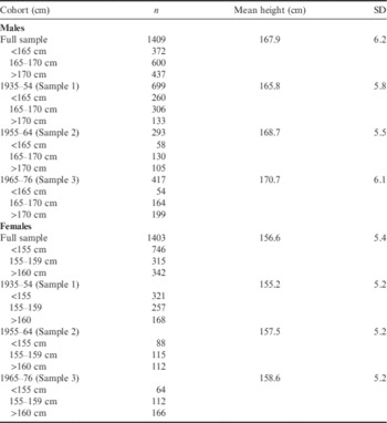
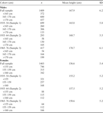
In 2003 the PSFD conducted a lifetime marriage history survey for Samples 1 and 2. This survey provides detailed information about an individual’s age at the outset and end of each marriage. Samples 1 and 2 (892 males and 982 females) are used to explore the age of first marriage and the history of having a partner in their lifetime. Samples 1 to 3 are used to investigate the current status of having a partner and children. Table 1 presents the height distribution and descriptive statistics of Samples 1 to 3. The younger generations are taller than the older generations.
Height distribution and statistical description of sample by sex and cohort
In the empirical work presented below, educational attainment is divided into three groups: high school and below, junior college and college and more, with high school and below being the reference group. Income provides resources information at the time of the survey, with current income being used as a proxy for long-term earnings. Region is divided into five categories: eastern, northern, central, southern, other regions and missing region (no answer given).
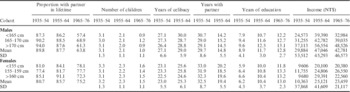
Table 2 shows the relation between height and reproductive success, as well as that between height and achievement (years of education and income). With the exception that taller males in cohort 1935–54 have a higher probability of marrying at least once, there seems to be no positive relation between height and other characteristics of reproductive success in any cohort. However, these results do not control other factors. It is a convention for Taiwanese to plan their marriages for when males have a stable job. Consequently, highly educated males usually marry late, and hence have a longer period of celibacy and shorter period of having a partner. Table 2 does demonstrate that tall males, on average, have higher educational attainment and earn more, but this is not the case for females. Stulp et al. (Reference Stulp, Pollet, Verhulst and Buunk2012a) pointed out that education and income are the most influential confounding factors when investigating the relation between height and reproductive success, but only very few previous studies have controlled these two factors. Stulp et al. (Reference Stulp, Pollet, Verhulst and Buunk2012a) indicated that education is actually detrimental to reproductive success for males. Nettle (Reference Nettle2002) suggested that males of higher social status are usually taller and have smaller families. The next section describes how regression analysis models controlling education and income are used to examine the relation between height and reproductive success.
Height and reproductive success and achievement by sex and cohort
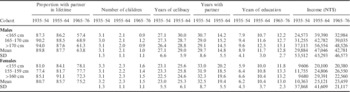
Age at first marriage, years of celibacy and years with partner are not available for cohort 1965–76.
NT$ is New Taiwan dollar; one US$ is approximately equal to 30 NT$.
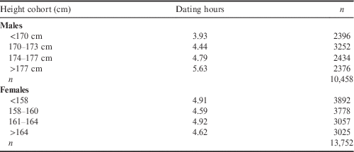
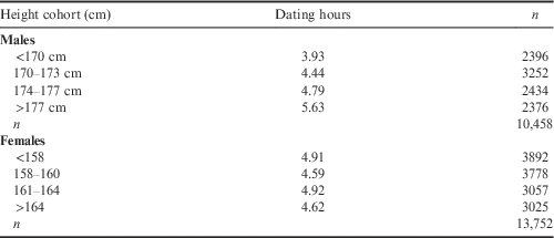
The data used to investigate the relation between height and dating hours are from the Taiwan Integrated Postsecondary Education Database (TIPED) compiled by the Center for Educational Research and Evaluation, National Taiwan Normal University. This is a nationally representative data set compiled in 2005. Roughly 25% of the population of college junior students was sampled; that is, 49,609 students. Of these, 26,307 responded to the questionnaire. After deleting missing data, 24,210 observations remained. The TIPED asked respondents to report their height and how many hours they dated per week. Table 3 divides the observations into four height groups. For males, the number of dating hours increases with height, but there is no linear relation for females.
Height and dating hours per week by sex
Mediation analyses and cohort effects
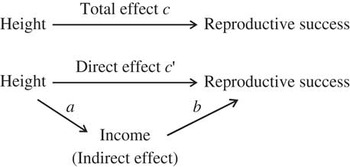
Taiwan has experienced fast economic development, and income per capita is negatively associated with infant mortality. It is possible that height has different effects on mate selection during different economic development periods. To further explore this possibility, the relation between height and reproductive success is probed for the three study cohorts separately. In addition, mediation analyses are conducted to further examine if height has a direct effect (c' in Fig. 1) or an indirect effect (a×b in Fig. 1) in increasing tall individuals’ reproductive success. The direct effect means that tall people are attractive, and height per se increases reproductive success. The indirect effect combines the effect of height on resources (income) and the effect of resources on reproductive success. Three necessary conditions must be met to claim that income (mediator) transmits the effect of height to reproductive success. These are that a and b are respectively significant, and the relationship between height and reproductive success diminishes as income is added into the model (Baron & Kenny, Reference Baron and Kenny1986; Little et al., Reference Little, Card, Bovaird, Preacher and Crandall2007).
Direct and indirect effects of height on reproductive success.

Suppose the total effect of height on reproductive success is c in Fig. 1, and the effect turns out to be c' if income is incorporated into the model. Technically, with the mediating effect in Fig. 1, the magnitude of c' is smaller and less significant than c. If the relationship between height and reproductive success is fully medicated, then c is statistically significant, while c' is statistically insignificant, and a×b is significant. A partial mediation is indicated, as c and a×b are significant but c' is weakly significant. Baron and Kenny (Reference Baron and Kenny1986) suggested that the first step in mediation analysis is to show that height is significantly related to reproductive success. That is, c is significant in the regression in Fig. 1. However, Shrout and Bolger (Reference Shrout and Bolger2002) argued that the test of c has a limited power for distal mediation, in which the effect of b is more substantial than the effect of a. They recommended that a mediation analysis proceeds on the basis of the strength of the theoretical argument rather than on the basis of the statistical test of c. In the present study, the effect of income (resources) on reproductive success is more substantial than the effect of height on income. Since income can be attributed to a distal mediator in this case, the insignificance of c does not hinder the examinations of the direct effect (c') and indirect effect (a×b) to claim that height medicates income to increase reproductive success.
The estimated indirect effect is
 $\hat{a}{\times}\hat{b}$
, where
 $\hat{a}$
and
 $\hat{b}$
are estimators of a and b, respectively. In a large sample, its standard error of the estimated indirect effect can be calculated as
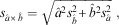 $$s_{{\hat{a}{\times}\hat{b}}} =\sqrt {\hat{a}^{2} s_{{\hat{b}}}^{2} {\plus}\hat{b}^{2} s_{{\hat{a}}}^{2} } }\ ,$$
where
 $s_{{\hat{a}}}^{2} $
and
 $s_{{\hat{b}}}^{2} $
are standard errors of
 $\hat{a}$
and
 $\hat{b}$
, respectively, and
 $\hat{a}{\times}\hat{b}/s_{{\hat{a}{\times}\hat{b}}} $
is approximately the Z-value in a large sample.
Regressions of height on mate selection and reproductive success
Following the mediation analysis in the previous section, this section investigates several issues regarding the relationships between height and mate selection and between height and offspring. Specifically, probit models are used to analyse the probabilities of having a partner and having at least one child, a Poisson model to explore the number of children and survival models to investigate the duration of celibacy before first marriage and duration of having a partner in the lifetime they currently have. An OLS model for age at first marriage and a survival model for duration of celibacy seem to be the same, but there are differences between the two samples. Respondents who are never married are deleted in the former sample, which could lead to a selection problem. However, the survival model is able to include respondents who are not married.
If males’ height plays a role in mate selection, then height is expected to be positively associated with the probability of having a partner and a child, the number of children and the duration of having a partner in one’s lifetime, while height is negatively correlated with the duration of celibacy. Moreover, tall males taking advantage of mate selection can be attributed to the resources link or the height per se link. Income is used here to represent the resources link. Occupations are also considered in all the models, but most categories are not significant and do not change the conclusions, so the final models do not incorporate these.
Although education is also resource-related, its resource capacity is fully absorbed by income. In the regressions below, income is excluded from the model of total effect but included in the model of direct effect, as shown in Fig. 1. In addition to height, the explanatory variables of the total effect model include age, educational attainment and regions. The direct effect model includes the same explanatory variables, but it also adds the explanatory variable of income. Coefficient b is the income coefficient in the direct effect model. Coefficient a comes from the regression of income on height, and this model has the same set of explanatory variables as the total effect model, but incorporates age squared to capture the inverse U-shaped relation between age and income. The magnitudes of the height coefficients and the degree of their significance in the total effect model reflect the combined effect of resources (indirect effect) and height per se (direct effect) links. When the coefficient of height of the total effect (c) and
 $$\hat{a}{\times}\hat{b}$$
are significant, and the magnitude of the direct effect (c') is smaller than c and is insignificant or less significant than c, height mediates income to enhance reproductive success. That is, the indirect effect matters. If c' is significant, the direct effect matters. With insignificant
 $$\hat{a}{\times}\hat{b}$$
and significant c', the height per se, instead of the domination of resources, influences mate selection.
The results of the mediation analysis of the full sample are shown below, followed by a discussion of the mediation of the cohort samples.
Probability of having at least one partner
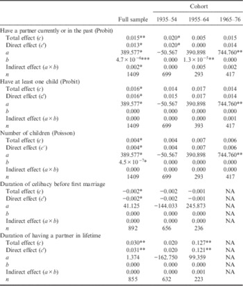
The top panel of Table 4 investigates the relationship between height and having at least one partner currently or in the past. The subjects could be married, divorced or widowed. The probit result for the total effect of height is positive and significant for males at the 5% level. The direct effect and the indirect effect are both positively significant at the 10% level. The sum of the direct and the indirect effects is equal to the total effect. The significant direct effect and indirect effect, respectively, indicate that height per se is positively associated with mate selection and that height influences mate selection through income. Tall males are less likely to be single, ceteris paribus.
Analyses of mediation effects of height on mate selection and reproductive success by cohort for males
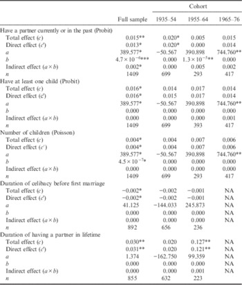
a is the regression coefficient of income on height, and b is the regression coefficient of reproductive success on income. The results of other explanatory are not shown.
NA: data not available.
Significance levels: ***1%, **5% and *10%.
The marginal effect of a probit model is probability change due to a 1 cm increment change in height. The probit model is a non-linear model, and its marginal effect varies with height. The marginal effect of probability for a probit model is ϕ(z)β height, where ϕ is the density function of a standard normal distribution function, z is a predicted value and β height is the coefficient of height. The marginal effect of probability has the same sign as β height. The coefficients presented in Table 4 are not the marginal effects, but the marginal effects have the same signs as the coefficients. Statistical software provides the marginal effect at average male height. The direct marginal effect of height is 0.003, which indicates that a 1 cm increment on height increases the probability by 0.003 for a male having a partner in their lifetime. The indirect marginal effect is 0.00044, which has a similar interpretation to the direct effect.
However, the significant direct and indirect effects do not occur consistently in the three cohorts. The oldest cohort (1935–54) continuously shows a significant direct effect, but the indirect effect is not significant. The direct and indirect effects are insignificant for cohorts 1955–64 and 1965–76; even b and a are significant for the former cohort and the latter cohort, respectively. It can be interpreted that the significance of the direct effect of the full sample comes from cohort 1935–54, while the significance of the indirect effects of the full sample comes from cohorts 1955–64 and 1965–76.
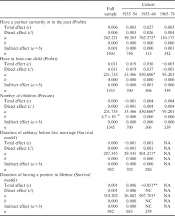
The top panel of Table 5 presents the same characteristics of mate selection for females as the top panel of Table 4. None of the direct and the indirect effects is significant for the full sample and the subsamples for females. Although males’ height is a useful characteristic in attracting females in mate selection, height is not a useful factor for females.
Analyses of mediation effects of height on mate selection and reproductive success by cohort for females
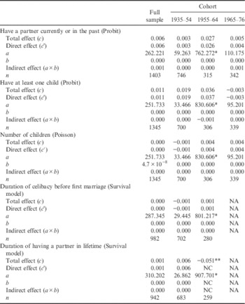
a is the regression coefficient of income on height, and b is the regression coefficient of reproductive success on income. The results of other explanatory are not shown.
NA: data not available; NC: survival models do not converge.
Significance levels: ***1%, **5% and *10%.
Probability of having at least one child
The second panel of Table 4 shows the probit results for males having at least one child. For the full sample, the direct effect is significant at the 10% level, while the indirect effect is insignificant. The indirect effect is not significant, although a is significant at the 10% level. The direct marginal effect at average male height is 0.002; that is, an incremental increase in height of 1 cm increases the probability of a male having at least one child by 0.002. Tall males are more likely to have offspring. This is not because tall males can provide more resources, but because height per se is related to males’ reproductive success. The significant direct effect does not occur in the subsamples. Table 5 shows that none of the direct and the indirect effects of height significantly increases the likelihood of females having at least one child.
Number of children
The third panel of Table 4 presents the Poisson results for males regarding number of children. For the full sample, the direct effect of height is positive and significant at the 10% level. The coefficient shown in Table 4 is also the marginal effect, indicating that an incremental increase in height of 1 cm increases males’ number of children by 0.004. The indirect effect is not significant, even though both a and b are significant at the 10% level. The close magnitudes of the total and the direct effects suggest that resources cannot explain the reproductive success of tall males. Tall males have more children because of height per se. The third panel of Table 5 shows that none of the direct and indirect effects is significant for females. Even when the infant mortality rate in Taiwan was substantially higher in earlier decades, tall women of the older cohort did not have more children than their counterparts. In 2003, the PSFD asked each mother respondent to report the number of her babies that died before they were one year old. Of the 3463 babies born to the female samples, 40 died before they were one year old. The infant mortality rate for the female sample is 1.16%, which is between 4.6% in 1958 and 0.36% in 2014. After considering the babies that died, in the PSFD data, only two women shifted from the childless category to having at least one child. After considering the babies that died, the probit model of having at least one child and the Poisson model of the number of children were re-analysed. Height is still insignificant for females’ reproductive success in these two models.
Duration of celibacy before first marriage (survival model)
Since marriage history was not surveyed for the youngest sample (1965–76), the youngest sample is not included. The observations used in the fourth and fifth panels of Tables 4 and 5 are fewer than those used in the first three panels. The current celibacy status might not persist in the future, and single people might be married in the future if the observed length of time is sufficiently long. Thus an OLS model deleting single people from the sample might give rise to the problem of non-randomness. Survival models are models of the length of time spent in a given status before transitioning to another status, and allow those single people to be considered in the model. The ‘status’ in some medical research is ‘alive’. When patients die, the status transitions from life to death. The ‘status’ in the survival model is celibacy. Being married means the end of the celibate status.
Several distributions are assumed to characterize the relationship between the duration time and hazard rate and the probability of leaving the initial status. These distributions are the exponential, the Weibull, the log-normal, the log-logistic and the Gamma distributions. Of these, the log-normal, the log-logistic and the Gamma distributions allow the hazard rate to first increase and then decrease. The hazard rate for the Weibull distribution is monotonically increasing or decreasing, while that for the exponential distribution is constant. Since age at marriage is frequently within the 20–30 years old range, the hazard rate regarding ending celibacy first increases and then decreases, which is consistent with the characteristics of the log-normal, log-logistic and Gamma distributions. These three distributions meet the study’s estimation requirements. The estimation results justify the inference. That is, the estimation results of the exponential and Weibull distributions are not reasonable. In Taiwan, education delays marriage, but the results of the exponential and Weibull distributions show that the coefficients of education are either significantly negative or insignificant. Furthermore, the generalized Gamma distribution is a generalized form of the exponential, Weibull and log-normal distributions. Since the results of the log-normal, log-logistic and generalized Gamma distributions are very similar, the fourth panel of Table 4 reports only the results of the generalized Gamma distribution. The height coefficients for both the total and the direct effects are the same, and they are negative and significant at the 10% level for males, implying that the resource link cannot explain why tall males are married earlier than short males, ceteris paribus. A negative coefficient in a survival model suggests it takes a shorter time to leave celibacy. The direct effect is –0.002, suggesting that the duration of celibacy reduces by 0.2% when males’ height increases by 1 cm. Similar to the previous results, neither the direct nor the indirect effects in the fourth panel in Table 5 for females are significant.
Duration of having a partner in one’s lifetime (survival model)
Finally, the study investigates the relationship between height and the length of time of having a partner in an individual’s lifetime. Not all subjects completely filled in their marriage history. The number of observations is less than that of the fourth panel. As in the case of the fifth panel of Tables 4 and 5, the survival model of the generalized Gamma distribution is applied. Again, the magnitudes of the total and direct effects are similar for males. Tall males have a longer time duration of living with a partner in their current lifetime because of height per se. The coefficient of the direct effect is 0.031, indicating that the time duration of having a partner in their lifetime increases by 3.1% when males’ height increases by 1 cm. Likewise, the last panel of Table 5 demonstrates that females’ height is irrelevant to their mate selection.
Stulp et al. (Reference Stulp, Pollet, Verhulst and Buunk2012a), Manfredini (2013) and Stulp et al. (Reference Stulp, Mills, Pollet and Barrett2014) indicated that the relationship between males’ height and their number of children is curvilinear. Males of average height have more children. Stulp et al. (Reference Stulp, Pollet, Verhulst and Buunk2012a) tested the relation between height and reproductive success (number of children ever born) by using the male data employed by Damon and Thomas (Reference Damon and Thomas1967) and found a curvilinear relation, which was not tested by Damon and Thomas (Reference Damon and Thomas1967). Mueller (Reference Mueller1979) concluded that there was a curvilinear relation from analysis of the principal components, of which height is the most important element. The theory suggests that males of average height being more attractive is stabilizing selection in which genetic variation is narrowed and stabilized, making the population more uniform. By contrast, directional selection means that mate selection moves genes in a certain direction – in this study’s case, tallness. This study therefore tested height squared in all the models of the full samples. However, while adding height squared did not change the significance of the coefficients for females in all of the models, it did result in both the coefficients of height and height squared being insignificant for males in all models. More importantly, Fig. 1 shows that adding height squared into the model makes the mediation analysis unable to linearly decompose into direct and indirect effects. In the section on height and dating hours, height squared will be incorporated into the model.
Table 4 shows that all the direct effects of the full sample are significant but most of their indirect effects are insignificant. This leads to the conclusion that height per se explains tall males’ reproductive success. However, this conclusion cannot be duplicated in the cohort subsamples. It appears that the conclusion from the full sample is not robust. Alternatively, the insignificance of height in the subsamples is likely to be a consequence of the weak significance of height in the full sample and smaller sample size of the subsamples. The smaller sample size of the subsamples cannot support the weak significance of height in the full sample. The smaller sample size enlarges the standard error of the coefficients of height, and the greater standard error reduces the degree of the significance of the height coefficient in the subsamples. This can be evidenced by the subsamples’ insignificant direct effects, which have the same magnitudes and the same signs as the weakly significant direct effects in the full samples. The magnitudes of observed significant direct effects in the subsamples (the top panel for cohort 1935–54 and the bottom panel for cohort 1955–64 in Table 4) are greater than the magnitudes of the direct effects in the full samples. This argument is in agreement with Shrout and Bolger (Reference Shrout and Bolger2002), who indicated that a small effect needs a large sample to be detected. Similarly, Stulp et al. (Reference Stulp, Pollet, Verhulst and Buunk2012a) stressed that small sample sizes have insufficient statistical power to detect height’s effect.
The modern human’s initial mate selection does not necessarily lead to marriage or reproduction. Therefore, the next section will explore the relation between height and dating hours. A large college student sample is used to avoid the low statistical power of a small sample size.
Dating and height
College students’ dating hours probably vary with their academic characteristics and family background. Students in some colleges or studying some subjects (majors) need to devote more time to their studies in order to pass exams. There are four types of colleges in Taiwan: public colleges, private colleges, public technological colleges and private technological colleges. In general, high school graduates advance to general colleges, while vocational high school graduates advance to technological colleges. Generally speaking, general colleges are more competitive than technological colleges, and public colleges are more competitive than private colleges. Students in public college usually allocate more time to studying, and hence have less time to date. By contrast, students in private technological college are likely to allocate more time to dating.
College majors are classified into nine groups: business, social science, literature, law, science, medicine, engineering, media and others. The ‘others’ category includes agriculture, home economics, tourism and physical education. Students that major in science, medicine or engineering need to dedicate more time to studying, and it is expected that these students spend less time dating.
Family income is divided into six groups, with income less than 500,000 New Taiwan dollars being the reference. Finally, college students who live at home are not as free as those who live in other locations. It is expected that students living at home will have fewer dating hours.
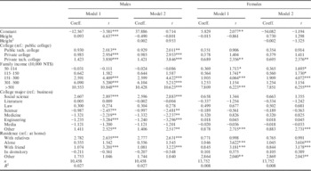
Table 6 presents the results of the regression of dating hours on height by sex for the two models, the difference between the models being that one includes height squared. When height squared is incorporated into the model, both height and its square are insignificant for both sexes. Consequently, the results of the height linear model are discussed. The results demonstrate that taller males have more dating hours, while height is irrelevant to females’ dating hours. Male students in public college have significantly fewer dating hours, and female students at private technological colleges have significantly more dating hours. The higher the family income, the more the dating hours. In economics terminology, dating is a type of luxury good. Family income is more influential for male than female students, probably because it is the convention in Taiwan for males to pay the bill on dates. Males’ dating hours are more sensitive to college majors than those of females’. Male college students whose majors require intensive study (science, medicine and engineering) date less than students majoring in business. Male students majoring in social science and both sexes majoring in other disciplines have longer dating hours. Finally, male college students living at home date less than those living with relatives or friends. Female college students living alone, with friends or with others date more than female students living at home.
Regression results for dating hours on height and sex
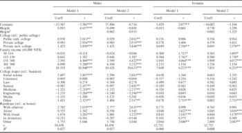
Significance levels: ***1%, **5% and *10%.
Accordingly, taller male college students are preferred by females. Unlike the weak significance or insignificance of height on males’ mate selection and reproductive success in previous regression results, male college students’ height is strongly related to their dating hours. One possible reason for the inconsistency is that dating does not necessarily lead to marriage or reproduction. Males’ height is strongly associated with dating hours, but it is not correlated with reproductive success. The other possibility is that dating still leads to reproductive success, but the college student cohort in Table 6 is too young to observe their consequential reproductive success. In this case, height plays a more important role in mate selection for a young cohort. However, the young cohort in the PSFD does not show this pattern. Alternatively, the college student sample is sufficiently large to detect the effect of height on mate selection, which cannot be detected in smaller samples.
Discussion and Conclusion
Personal traits that are positively associated with earnings or resources give males an advantage when it comes to mate selection. The study uses mediation analyses to discern the direct and indirect effects of height on males’ reproductive success. The full sample is divided into three cohort samples to examine whether this weak relation between height and reproductive success persists in all subsamples. For the male full sample the direct effects are verified for all characteristics of mate selection and reproductive success. More specifically, ceteris paribus, tall males are more likely to have a partner and have at least one child, and have more children, a shorter period of celibacy and a longer duration of living with a partner in their current lifetimes. Notably, most of the degrees of significance are only at the 10% level. The conclusions apply to males but not to females. Stulp et al. (Reference Stulp, Verhulst, Pollet and Buunk2012b) reported that females’ height is detrimental to their reproductive success in Western populations, but their study results are inclusive about females’ reproductive success in non-Western populations. Although Taiwanese males’ height is a characteristic of sexual dimorphism in attracting females in mate selection, height is not a significant factor for Taiwanese females.
The significant direct effects for males disappear in most subsamples. This suggests that the insignificant relations in the subsamples are a consequence of the weak relation in the full sample and small sample size of the subsamples. The sample size and their variation in the subsamples decline, and their standard errors increase. It is unfortunate that the study’s sample is not sufficiently large to explore how the relation between height and reproductive success varies over cohorts. Moreover, several decades ago, impoverished Taiwanese citizens had little savings and insufficient Social Security. The elderly were looked after by their adult children. The more children the elderly had, the more likely they were to be sufficiently taken care of. Consequently, the elderly with reproductive success are likely to live longer. While investigating the relationship between reproductive success and height, regardless of how tall the elderly were, those with more adult children were more likely to be surveyed. As a result, the relationship between height and reproductive success attenuates towards zero. This is because only the elderly with more adult children are observed, regardless of their height. However, since the oldest respondents in the survey are only 69 years old, the weak and the insignificant relations between height and reproductive success might not be due to this problem.
Finally, dating is the first step in mate selection. This study uses a large sample to investigate the relationship between height and dating hours. Since modern humans do not necessarily get married or desire to have children, to probe the relation between height and mate selection, an investigation of dating hours might be more appropriate. A large college student sample is employed to explore the relation between height and dating hours and to avoid the low statistical power of detection. Tall male students have significantly more dating hours than short male students. Unlike the weakly significant relation between height and mate selection and between height and reproductive success for the PSFD adult sample, the relation between height and dating hours is strong for male college students. Again, this relation is not significant for female students. College students do not have formal jobs, so mediation analysis is not possible. However, students’ academic characteristics and their potential earning capacities are controlled. Therefore, this implies that females prefer tall college male students not because of their resources, but because of height per se.