1. Introduction
Nonlinear interplay of energetic particles (EP) with Alfvénic fluctuations, such as Alfvén eigenmodes (AE), EP modes and drift Alfvén waves (Chen & Zonca Reference Chen and Zonca2007; Fasoli et al. Reference Fasoli, Gormenzano, Berk, Breizman, Briguglio, Darrow, Gorelenkov, Heidbrink, Jaun, Konovalov, Nazikian, Noterdaeme, Sharapov, Shinohara, Testa, Tobita, Todo, Vlad and Zonca2007; Chen & Zonca Reference Chen and Zonca2013, Reference Chen and Zonca2015), and their consequences for fluctuation induced cross-field transport constitute basic phenomena for thermonuclear plasmas (Fasoli et al. Reference Fasoli, Gormenzano, Berk, Breizman, Briguglio, Darrow, Gorelenkov, Heidbrink, Jaun, Konovalov, Nazikian, Noterdaeme, Sharapov, Shinohara, Testa, Tobita, Todo, Vlad and Zonca2007; Heidbrink Reference Heidbrink2008; Breizman & Sharapov Reference Breizman and Sharapov2011; Wang et al. Reference Wang, Briguglio, Chen, Di Troia, Fogaccia, Vlad and Zonca2011; Schneller et al. Reference Schneller, Lauber, Brüdgam, Pinches and Günter2012, Reference Schneller, Lauber, Bilato, García-Muñoz, Brüdgam and Günter2013; Lauber Reference Lauber2013; Vlad et al. Reference Vlad, Briguglio, Fogaccia, Zonca, Fusco and Wang2013; Gorelenkov, Pinches & Toi Reference Gorelenkov, Pinches and Toi2014; Pinches et al. Reference Pinches, Chapman, Lauber, Oliver, Sharapov, Shinohara and Tani2015; Zonca et al. Reference Zonca, Chen, Briguglio, Fogaccia, Milovanov, Qiu, Vlad and Wang2015a ,Reference Zonca, Chen, Briguglio, Fogaccia, Vlad and Wang b ). The relevance of the beam–plasma instability problem as paradigm for EP transport due to AE was proposed in Berk & Breizman (Reference Berk and Breizman1990a ,Reference Berk and Breizman b ,Reference Berk and Breizman c ). In fact, the bump-on-tail paradigm can mimic the nonlinear interaction of supra-thermal particles with Alfvénic fluctuations, provided the system is sufficiently close to marginal stability (Berk & Breizman Reference Berk and Breizman1990c ; Chen & Zonca Reference Chen and Zonca2007, Reference Chen and Zonca2013; Breizman & Sharapov Reference Breizman and Sharapov2011). In particular, it is possible to determine a correspondence between velocity space transport in the one-dimensional (1-D) beam–plasma instability problem and radial transport of fast ions in the presence of resonant AE, at least as far as their spatial structure does not play a significant role. More precisely, such correspondence has a rigorous foundation as long as the nonlinear resonant particle displacement is small compared to the characteristic perpendicular fluctuation scale (Wang et al. Reference Wang, Briguglio, Chen, Di Troia, Fogaccia, Vlad and Zonca2012; Briguglio et al. Reference Briguglio, Wang, Zonca, Vlad, Fogaccia, Di Troia and Fusco2014; Chen & Zonca Reference Chen and Zonca2015; Zonca et al. Reference Zonca, Chen, Briguglio, Fogaccia, Milovanov, Qiu, Vlad and Wang2015a ,Reference Zonca, Chen, Briguglio, Fogaccia, Vlad and Wang b ).
The beam–plasma instability was analysed in the pioneering works of O’Neil and collaborators (O’Neil & Malmberg Reference O’Neil and Malmberg1968; O’Neil, Winfrey & Malmberg Reference O’Neil, Winfrey and Malmberg1971) (see also Shapiro Reference Shapiro1963; Onishchenko et al. Reference Onishchenko, Linetskii, Matsiborko, Shapiro and Shevchenko1970; Shapiro & Shevchenko Reference Shapiro and Shevchenko1971; Thompson Reference Thompson1971; Levin et al. Reference Levin, Lyubarskiǐ, Onishchenko, Shapiro and Shevchenko1972; Matsiborko et al. Reference Matsiborko, Onishchenko, Shapiro and Shevchenko1972). It was analysed for a nearly monochromatic fast electron beam injected into a 1-D plasma, which, in turn, is treated as a linear dielectric medium supporting longitudinal Langmuir waves (Lifshitz & Pitaevskii Reference Lifshitz and Pitaevskii1976). It was demonstrated that Langmuir fluctuations can be resonantly excited by EP and become unstable. The original approach of O’Neil et al. (Reference O’Neil, Winfrey and Malmberg1971) can be cast in a rigorous Hamiltonian formulation (Mynick & Kaufman Reference Mynick and Kaufman1978; Tennyson, Meiss & Morrison Reference Tennyson, Meiss and Morrison1994; Antoni, Elskens & Escande Reference Antoni, Elskens and Escande1998); and the resulting scheme is formally equivalent to that of Free-Electron Laser dynamics (Antoniazzi et al. Reference Antoniazzi, Johal, Fanelli and Ruffo2008). An alternative approach was given in Al’Tshul’ & Karpman (Reference Al’Tshul’ and Karpman1966), where the nonlinear Vlasov–Poisson initial value problem was solved for the case of nearly degenerate Langmuir and beam modes and an analogue of the Dyson equation was derived (see Chen & Zonca (Reference Chen and Zonca2015), Zonca et al. (Reference Zonca, Chen, Briguglio, Fogaccia, Milovanov, Qiu, Vlad and Wang2015a ,Reference Zonca, Chen, Briguglio, Fogaccia, Vlad and Wang b ) for an in-depth discussion of this approach). An example of the beam–plasma instability in the presence of more than a single resonant mode was analysed by Zaslavsky et al. (Reference Zaslavsky, Krafft, Gorbunov and Volokitin2008), emphasizing the link with the so-called sideband instability, and addressing a simple Hamiltonian formulation of the problem. Meanwhile, Evstatiev, Horton & Morrison (Reference Evstatiev, Horton and Morrison2003) also include the effect of a magnetic field in the multi-wave model, but the analysis refers to a single longitudinal resonant electrostatic mode. Pioneering works on these thematics can be found in Deneef (Reference Deneef1975) and in Lacina, Krlín & Körbel (Reference Lacina, Krlín and Körbel1976), where 1-D beam–plasma interaction with higher harmonics has been studied.
The beam–plasma problem is characterized by typical velocity and temporal scales. Nonlinear saturation of the beam–plasma instability occurs over a
 ${\sim}{\it\gamma}_{L}^{-1}$
characteristic time, with
 ${\it\gamma}_{L}$
the linear instability growth rate (O’Neil & Malmberg Reference O’Neil and Malmberg1968); while beam heating typically takes place at a rate
 ${\sim}{\it\omega}_{B}\propto |ek^{2}{\it\varphi}/m_{e}|^{1/2}$
, i.e. the wave–particle trapping frequency in the fluctuating scalar potential
 ${\it\varphi}$
with wave number
 $k$
(here
 $m_{e}$
and
 $e$
denote the mass and charge of electrons, respectively) and involves resonant particles in an interval
 ${\rm\Delta}v\sim {\it\omega}_{B}/k\sim ({\it\omega}_{B}/{\it\omega}_{p})v_{B}$
about the velocity resonance condition
 $v=v_{B}$
(where
 $v_{B}$
is the EP drifting beam velocity). The saturation level of the beam–plasma instability can be estimated as
 ${\it\omega}_{B}\sim 3{\it\gamma}_{L}$
(O’Neil et al.
Reference O’Neil, Winfrey and Malmberg1971; Levin et al.
Reference Levin, Lyubarskiǐ, Onishchenko, Shapiro and Shevchenko1972), while the flattening of the beam distribution function can take much longer times than
 ${\sim}{\it\omega}_{B}^{-1}$
and involves the formation of structures in the wave–particle trapping region (Tennyson et al.
Reference Tennyson, Meiss and Morrison1994). It has been recently shown (Carlevaro et al.
Reference Carlevaro, Fanelli, Garbet, Ghendrih, Montani and Pettini2014) that the nonlinear evolution of the beam–plasma system is characterized by quasi-stationary states which can be accurately predicted by the maximum entropy principle proposed by Lynden–Bell (Antoni et al.
Reference Antoni, Elskens and Escande1998).
In the present work, we formulate the general problem of
 $n$
cold beams self-consistently evolving in the presence of
 $m\geqslant n$
unstable modes degenerate with the Langmuir potentials at the plasma frequency
 ${\it\omega}_{p}$
, i.e.
 ${\it\omega}={\it\omega}_{p}$
, which ensures that the dielectric function of the cold background plasma is nearly vanishing. Among these waves, we can select
 $n$
modes which are resonantly driven by the beams (obeying to the O’Neil selection rule
 $k={\it\omega}_{p}/v_{B}$
(O’Neil & Malmberg Reference O’Neil and Malmberg1968; O’Neil et al.
Reference O’Neil, Winfrey and Malmberg1971)) and
 $m-n$
quasi-degenerate ones associated with nonlinear wave–particle and/or mode–mode coupling in the case of (almost) overlapping resonances. It is worth noting that the dominant quasi-degenerate modes can also be dealt with as slowly evolving Langmuir waves when the spectral density is sufficiently large. In particular, we will show in § 3 that nonlinear excitation of quasi-degenerate sidebands can be important for the case of two interacting beams.
The physical motivation for the proposed model relies on the fact that, due to the intrinsic beam heating involved in the nonlinear beam–plasma dynamics (Shapiro Reference Shapiro1963), transport is not qualitatively different for cold and warm beams as long as the initial beam width in velocity space is smaller than
 ${\rm\Delta}v$
. Thus transport in the presence of overlapping resonances may be studied as the evolution of initially cold beams as a consequence of the corresponding nearly degenerate beam (Langmuir) instabilities. This statement justifies the representation of the bump-on-tail problem in terms of
 $n$
overlapping resonances and has the valuable feature of maintaining direct control on spectral density and intensity, which are the properties that ultimately determine EP transport.
The proposed theoretical model can properly describe the case of isolated resonances and
 $m=n$
uncoupled nonlinear oscillators (dominated by wave–particle trapping), as well as the ‘quasi-linear’ diffusion regime typical of a ‘broad fluctuation spectrum’ (Al’Tshul’ & Karpman Reference Al’Tshul’ and Karpman1966). In fact, the nonlinear equation system we propose, in the limit of very large
 $n$
, is expected to be physically isomorphic to quasi-linear models of EP interaction with AE. In this respect, it is important to mention that a line-broadened quasi-linear approach has been proposed by Berk et al. (Reference Berk, Breizman, Fitzpatrick and Wong1995a
, Reference Berk, Breizman, Fitzpatrick, Pekker, Wong and Wong1996a
) for computing EP transport by means of a diffusion equation, which could address not only overlapping modes but also the broadening of the resonant spectrum for isolated instabilities in the case of multiple AE. This model has been extended and compared with experimental observations (Ghantous et al.
Reference Ghantous, Gorelenkov, Berk, Heidbrink and Van Zeeland2012) and with numerical solutions of the bump-on-tail paradigm (Ghantous, Berk & Gorelenkov Reference Ghantous, Berk and Gorelenkov2014). Contrary to this approach, which cannot account for frequency chirping phenomena (Ghantous et al.
Reference Ghantous, Berk and Gorelenkov2014), the present
 $n$
-beam model aims at characterizing particle transport on a time scale comparable to the instability growth rate and thus it can address a broad range of underlying complex phenomena (Chen & Zonca Reference Chen and Zonca2015; Zonca et al.
Reference Zonca, Chen, Briguglio, Fogaccia, Milovanov, Qiu, Vlad and Wang2015a
,Reference Zonca, Chen, Briguglio, Fogaccia, Vlad and Wang
b
).
As an illustration of the onset of particle transport phenomena in the phase-space, the simulation discussed in this work are specialized to two cold beams and corresponding instabilities. Clearly, when the two beams have sufficiently different initial velocities, we observe the growth and saturation of two independent modes and transport processes are practically suppressed. Meanwhile, when the two velocities become closer, a regime exists when the slower beam significantly interacts with the resonant mode excited by the faster beam and an
 $O(1)$
transfer of energy from the latter mode to the former takes place. Finally, when the velocity ratio exceeds a critical threshold consistent with the Chirikov criterion (Levin et al.
Reference Levin, Lyubarskiǐ, Onishchenko, Shapiro and Shevchenko1972; Chirikov Reference Chirikov1979), significant phase-space mixing takes place between the two beam populations.
As we are interested in the details of the mixing process between supra-thermal particles belonging to different beams in the presence of unstable fluctuations, we will present an analysis using a Lagrangian approach in order to quantitatively define the transport barriers of the system by means of so-called Lagrangian Coherent Structures (LCS), introduced for the first time by Peacock & Haller (Reference Peacock and Haller2013) and defined in terms of the features of the Finite Time Lyapunov Exponent (FTLE) fields (Falessi, Pegoraro & Schep Reference Falessi, Pegoraro and Schep2015). For practical reasons, particle transport is described as the evolution of single passive tracers (test particles) in a time-dependent potential generated at each instant by the self-consistent charge distribution. This approach, which is equivalent to the original problem, leads to important conceptual simplifications if we are interested in studying the onset of an instability that naturally selects only some Fourier components. The advection of passive tracers in a non-periodic flow has been studied by Shadden, Lekien & Marsden (Reference Shadden, Lekien and Marsden2005), Haller (Reference Haller2011), leading to the definition of LCS. These structures, which are 1-D curves in our system, are finite-time transport barriers for the tracers and, therefore, play the role of the last periodic surface of the Poincaré map introduced in Shadden et al. (Reference Shadden, Lekien and Marsden2005), Haller (Reference Haller2011). Thus, they divide tracers into two classes with a qualitatively different evolution. This way of characterizing transport gives a criterion for the transition to local chaotic behaviour, i.e. for assessing when nonlinear dynamics causes neighbouring cold beams to merge.
The paper is organized as follows. In § 2, the nonlinear treatment of the beam–plasma system of O’Neil is generalized in the presence of
 $n$
distinct beams and
 $m$
nearly degenerate Langmuir modes. In § 3, the theoretical model is then specialized for the two beam case and, in the first subsection, for the corresponding two most unstable modes. Numerical simulations are presented first by analysing temporal evolutions of scalar potentials and then by discussing the phase-space dynamics. Mixing phenomena between different populations are qualitatively analysed as a function of the ratio between initial beam velocities. An analysis of quasi-degenerate modes including nonlinear sideband excitation is discussed in the second subsection. In § 4, transport processes are qualitatively studied by means of the LCS technique. Phase-space mixing is found to be enhanced at the intersections between LCS belonging to different beam populations. This analysis allows us to define a critical initial velocity ratio of beams as the smallest value leading to beam mixing. Concluding remarks are given in § 5.
2. Nonlinear evolution of
 $n$
resonant beams

In the original stability analysis of the beam–plasma system (O’Neil & Malmberg Reference O’Neil and Malmberg1968), it was shown how fluctuations can be resonantly excited by an injected supra-thermal beam (of velocity
 $v_{B}$
). Introducing the plasma frequency
 ${\it\omega}_{p}\equiv \sqrt{4{\rm\pi}n_{p}e^{2}/m_{e}}$
(
 $n_{p}$
being the plasma density), two types of modes were shown to exist as solutions of the dispersion relation: (i) the stable Langmuir wave with
 ${\it\omega}={\it\omega}_{p}$
, modified by the presence of EP; and (ii) the beam mode, with both stable and unstable branches at frequency
 ${\it\omega}\simeq kv_{B}$
, and a maximum growth rate when
 ${\it\omega}\simeq {\it\omega}_{p}$
(here,
 $k$
represents the wavenumber of the unstable longitudinal mode). Thus most unstable beam modes are excited when they are ‘nearly degenerate’ with Langmuir waves, i.e.
 $k\simeq {\it\omega}_{p}/v_{B}$
. Meanwhile, nonlinear evolution takes place in two stages (Shapiro Reference Shapiro1963; O’Neil et al.
Reference O’Neil, Winfrey and Malmberg1971): first, beam–plasma interactions heat the beam as EP begin sloshing back and forth in the potential well of the wave; and second, the beam distribution function is eventually flattened in velocity space by nonlinear interactions. Thus the process leading to saturation of the beam–plasma instability is due to wave trapping of resonant particles whose transport in velocity space is connected with energy exchange between fast electrons and the electric field.
In this section, we derive the governing equations for the general system of
 $n$
cold beams and
 $m\geqslant n$
self-consistently coupled modes (O’Neil et al.
Reference O’Neil, Winfrey and Malmberg1971). It is important to stress that all considered
 $m$
modes are assumed to be nearly degenerate Langmuir waves with close to vanishing dielectric function, while resonance conditions are not imposed a priori. The background plasma is a cold homogeneous linear dielectric medium with constant particle density
 $n_{p}$
. The dynamics of fast electrons is determined by the Newton’s law. Equations of motion are closed by the Poisson equation which provides the time evolution for each of the nearly degenerate Langmuir waves considered in the model.
In a 1-D model, the motion along the
 $x$
direction of period
 $L$
is labelled by
 $x_{1},x_{2},\dots ,x_{n}$
for each beam, respectively. Decomposing the single beams in
 $N_{1},N_{2},\dots ,N_{n}$
charge sheets located at
 $x_{1i},x_{2i},\dots ,x_{ni}$
, the system can be discretized using the following total charge density
 $$\begin{eqnarray}{\it\rho}_{B}(x,t)=-en_{B}\left(\frac{L{\it\sigma}_{1}}{N_{1}}\mathop{\sum }_{i=1}^{N_{1}}{\it\delta}(x-x_{1i})+\cdots +\frac{L{\it\sigma}_{n}}{N_{n}}\mathop{\sum }_{i=1}^{N_{n}}{\it\delta}(x-x_{ni})\right),\end{eqnarray}$$
where
 $n_{B}$
is the total supra-thermal particle number density while
 ${\it\sigma}_{1}n_{B},\dots ,{\it\sigma}_{n}n_{B}$
are the number densities of each beam. The Langmuir wave scalar potential can be expressed using the Fourier representation as
 $$\begin{eqnarray}{\it\varphi}(x,t)=\mathop{\sum }_{j=1}^{m}({\it\varphi}_{j}(k_{j},t)\text{e}^{\text{i}k_{j}x-\text{i}{\it\omega}_{p}t}+\text{c.c.}),\end{eqnarray}$$
where
 ${\it\varphi}_{j}(k_{j},t)$
are assumed to be slowly varying fields and we have explicitly indicated the time dependence relative to the rapid oscillations associated to the plasma frequency. Thus the
 ${\it\varphi}_{j}$
’s represent the effective nonlinear evolution of the potentials.
The trajectories of charge sheets are derived from the motion equation
 $\ddot{x}=e\boldsymbol{{\rm\nabla}}{\it\varphi}/m_{e}$
as
 $$\begin{eqnarray}\displaystyle \ddot{x}_{1i}=\frac{\text{i}\text{e}}{m}\mathop{\sum }_{j=1}^{m}k_{j}{\it\varphi}_{j}\text{e}^{\text{i}k_{j}x_{1i}-\text{i}{\it\omega}_{p}t}+\text{c.c.},\end{eqnarray}$$
 $$\begin{eqnarray}\vdots\end{eqnarray}$$
 $$\begin{eqnarray}\displaystyle \ddot{x}_{ni}=\frac{\text{i}\text{e}}{m}\mathop{\sum }_{j=1}^{m}k_{j}{\it\varphi}_{j}\text{e}^{\text{i}k_{j}x_{ni}-\text{i}{\it\omega}_{p}t}+\text{c.c.}\end{eqnarray}$$
 ${\it\varphi}_{j}$
is determined by the Poisson’s equation written in the Fourier space for fixed
 $k_{j}$
as
 $$\begin{eqnarray}k_{j}^{2}{\it\epsilon}_{p}{\it\varphi}_{j}\text{e}^{-\text{i}{\it\omega}_{p}t}=4{\rm\pi}\,{\it\rho}_{Bj}(k_{j},t),\end{eqnarray}$$
where
 ${\it\epsilon}_{p}$
is the dielectric function (we note that for a cold plasma
 ${\it\epsilon}_{p}=1-{\it\omega}_{p}^{2}/{\it\omega}^{2}$
) and
 ${\it\rho}_{Bj}(k_{j},t)$
is the Fourier transformed density
 $$\begin{eqnarray}{\it\rho}_{Bj}(k_{j},t)=\frac{1}{L}\int _{0}^{L}\,\text{d}x{\it\rho}_{B}(x,t)\text{e}^{-\text{i}k_{j}x}=-e\,n_{B}\left(\frac{{\it\sigma}_{1}}{N_{1}}\mathop{\sum }_{i=1}^{N_{1}}\text{e}^{-\text{i}k_{j}x_{1i}}+\cdots +\frac{{\it\sigma}_{n}}{N_{n}}\mathop{\sum }_{i=1}^{N_{n}}\text{e}^{-\text{i}k_{j}x_{ni}}\right).\end{eqnarray}$$
For a cold plasma and
 $j=1,2,\dots ,m$
nearly degenerate Langmuir waves, the dielectric function is nearly vanishing and can thus be expanded near
 $({\it\omega}_{p},k_{j})$
as
 $$\begin{eqnarray}{\it\epsilon}_{p}({\it\omega}(t),k_{j})={\it\epsilon}_{p}({\it\omega}_{p},k_{j})+(\partial {\it\epsilon}_{p}/\partial {\it\omega})|_{{\it\omega}_{p},k_{j}}({\it\omega}_{j}-{\it\omega}_{p})\equiv {\it\epsilon}^{\prime }({\it\omega}_{j}-{\it\omega}_{p}),\end{eqnarray}$$
where the time-dependent
 ${\it\omega}_{j}$
account for the nonlinear frequency shift with respect to
 ${\it\omega}_{p}$
. Without loss of generality, the fields
 ${\it\varphi}_{j}$
can be now expressed as
 $$\begin{eqnarray}{\it\varphi}_{j}(t)\propto \exp \left(-\text{i}\int _{0}^{t}\,\text{d}\bar{t}\,({\it\omega}_{j}(\bar{t})-{\it\omega}_{p})\right),\end{eqnarray}$$
thus obtaining
 $\dot{{\it\varphi}}_{j}=-\text{i}({\it\omega}_{j}-{\it\omega}_{p}){\it\varphi}_{j}$
; and equation (2.4) finally writes
 $$\begin{eqnarray}\dot{{\it\varphi}}_{j}=\text{i}\frac{4{\rm\pi}en_{B}}{k_{j}^{2}{\it\epsilon}^{\prime }}\left(\frac{{\it\sigma}_{1}}{N_{1}}\mathop{\sum }_{i=1}^{N_{1}}\text{e}^{-\text{i}k_{j}x_{1i}+\text{i}{\it\omega}_{p}t}+\cdots +\frac{{\it\sigma}_{n}}{N_{n}}\mathop{\sum }_{i=1}^{N_{n}}\text{e}^{-\text{i}k_{j}x_{1i}+\text{i}{\it\omega}_{p}t}\right).\end{eqnarray}$$
The equations of motion governing the beam–plasma system are (2.3) and (2.8).
Let us now analyse the effective nonlinear shift
 ${\it\zeta}$
of charge sheets due to the beam–wave interaction by decomposing the motion as
 $$\begin{eqnarray}x_{1i}=v_{1}t+{\it\zeta}_{1i}(t),\quad x_{2i}=v_{2}t+{\it\zeta}_{2i}(t),\quad \dots ,\quad x_{ni}=v_{n}t+{\it\zeta}_{ni}(t).\end{eqnarray}$$
Performing this coordinate transformation and introducing the scaled variables (recalling that for a cold plasma,
 ${\it\epsilon}^{\prime }=2/{\it\omega}_{p}$
)
 $$\begin{eqnarray}k_{j}=2{\rm\pi}\ell _{j}/L,\quad \bar{{\it\zeta}}_{ni}=2{\rm\pi}{\it\zeta}_{ni}/L,\quad {\it\tau}=t{\it\omega}_{p}\bar{{\it\eta}},\quad {\it\phi}_{j}=[{\it\varphi}_{j}ek_{j}^{2}]/[m\bar{{\it\eta}}^{2}{\it\omega}_{p}^{2}],\end{eqnarray}$$
with
 $\bar{{\it\eta}}=(n_{B}/2n_{p})^{1/3}$
and frequency mismatches
 $$\begin{eqnarray}{\it\beta}_{1j}=[k_{j}v_{1}-{\it\omega}_{p}]/{\it\omega}_{p}\bar{{\it\eta}},\quad \dots ,\quad {\it\beta}_{nj}=[k_{j}v_{n}-{\it\omega}_{p}]/{\it\omega}_{p}\bar{{\it\eta}},\end{eqnarray}$$
the set of equations describing the effective nonlinear dynamics of
 $n$
cold beams interacting with
 $m$
Langmuir modes reads now (the prime denotes the
 ${\it\tau}$
derivative)
 $$\begin{eqnarray}\displaystyle \bar{{\it\zeta}}_{1i}^{\prime \prime }=\text{i}\mathop{\sum }_{j=1}^{m}\ell _{j}^{-1}{\it\phi}_{j}\text{e}^{\text{i}\ell _{j}\bar{{\it\zeta}}_{1i}+\text{i}{\it\beta}_{1j}{\it\tau}}+\text{c.c.},\end{eqnarray}$$
 $$\begin{eqnarray}\vdots\end{eqnarray}$$
 $$\begin{eqnarray}\displaystyle & \displaystyle \bar{{\it\zeta}}_{ni}^{\prime \prime }=\text{i}\mathop{\sum }_{j=1}^{m}\ell _{j}^{-1}{\it\phi}_{j}\text{e}^{\text{i}\ell _{j}\bar{{\it\zeta}}_{ni}+\text{i}{\it\beta}_{nj}{\it\tau}}+\text{c.c.}, & \displaystyle\end{eqnarray}$$
 $$\begin{eqnarray}\displaystyle & \displaystyle {\it\phi}_{j}^{\prime }=\text{i}\left(\frac{{\it\sigma}_{1}}{N_{1}}\mathop{\sum }_{i=1}^{N_{1}}\text{e}^{-\text{i}\ell _{j}\bar{{\it\zeta}}_{1i}-\text{i}{\it\beta}_{1j}{\it\tau}}+\cdots +\frac{{\it\sigma}_{n}}{N_{n}}\mathop{\sum }_{i=1}^{N_{n}}\text{e}^{-\text{i}\ell _{j}\bar{{\it\zeta}}_{ni}-\text{i}{\it\beta}_{nj}{\it\tau}}\right). & \displaystyle\end{eqnarray}$$
 ${\it\beta}$
’s, implying that the most unstable modes associated to a given beam must obey the O’Neil selection rule
 $k_{j}=v_{j}/{\it\omega}_{p}$
. We stress how this dynamical system is isomorphic with respect to the model commonly adopted in a class of studies of wave–particle interactions and rigorously derived in Elskens & Escande (Reference Elskens and Escande2003) (see also Farina et al.
Reference Farina, Casagrande, Colombo and Pozzoli1994; Antoni et al.
Reference Antoni, Elskens and Escande1998; Firpo & Elskens Reference Firpo and Elskens2000; Farina & Pozzoli Reference Farina and Pozzoli2004; Antoniazzi et al.
Reference Antoniazzi, Elskens, Fanelli and Ruffo2006). For an example of the mapping between the beam–plasma instability and the Free-Electron Laser model see Antoniazzi et al. (Reference Antoniazzi, DeNinno, Fanelli, Guarino and Ruffo2005).
The conservation laws of the system above can be derived by extension of the method outlined by O’Neil et al. (Reference O’Neil, Winfrey and Malmberg1971). The total momentum conservation reads now
 $$\begin{eqnarray}\mathop{\sum }_{j=1}^{m}\frac{|{\it\phi}_{j}|^{2}}{\ell _{j}}+\frac{{\it\sigma}_{1}}{N_{1}}\mathop{\sum }_{i=1}^{N_{1}}\bar{{\it\zeta}}_{1i}^{\prime }+\cdots +\frac{{\it\sigma}_{n}}{N_{n}}\mathop{\sum }_{i=1}^{N_{n}}\bar{{\it\zeta}}_{ni}^{\prime }={\mathcal{K}}_{M},\end{eqnarray}$$
with constant
 ${\mathcal{K}}_{M}$
. As already stated in (2.7), the potentials obey to the equation
 $\dot{{\it\varphi}}_{j}=-\text{i}({\it\omega}_{j}-{\it\omega}_{p}){\it\varphi}_{j}$
, which can be simply rewritten as
 ${\it\phi}_{j}^{\prime }=-\text{i}{\it\Omega}_{j}{\it\phi}_{j}$
, where
 ${\it\Omega}_{j}\equiv ({\it\omega}_{j}-{\it\omega}_{p})/({\it\omega}_{p}\bar{{\it\eta}})={\it\delta}{\it\omega}_{j}/{\it\omega}_{p}\bar{{\it\eta}}$
. Using these expressions, total energy conservation can be cast in the following form
 $$\begin{eqnarray}\displaystyle & & \displaystyle \mathop{\sum }_{j=1}^{m}\frac{|{\it\phi}_{j}|^{2}}{\bar{{\it\eta}}\ell _{j}^{2}}+2\mathop{\sum }_{j=1}^{m}{\it\Omega}_{j}^{\mathit{Re}}\frac{|{\it\phi}_{j}|^{2}}{\ell _{j}^{2}}\nonumber\\ \displaystyle & & \displaystyle \quad +\,\frac{1}{2}\left[\frac{{\it\sigma}_{1}}{N_{1}}\mathop{\sum }_{i=1}^{N_{1}}(\bar{{\it\zeta}}_{1i}^{\prime }+2{\rm\pi}v_{1}/L\bar{{\it\eta}}{\it\omega}_{p})^{2}+\cdots +\frac{{\it\sigma}_{n}}{N_{n}}\mathop{\sum }_{i=1}^{N_{n}}(\bar{{\it\zeta}}_{ni}^{\prime }+2{\rm\pi}v_{n}/L\bar{{\it\eta}}{\it\omega}_{p})^{2}\right]\!={\mathcal{K}}_{E},\qquad \quad\end{eqnarray}$$
with constant
 ${\mathcal{K}}_{E}$
. These conservation laws are directly connected with the Hamiltonian representation of the system. Thus the present approach based on the motion of
 $N$
particles in the self-consistent Langmuir potentials is more general and reduces to the Vlasov–Poisson description in the mean field limit of the Hamiltonian formulation treated according to Klimontovich (Reference Klimontovich1967). The Vlasov–Maxwell equations are exactly recovered taking the continuum or mush limit, i.e. artificially increasing the number of particles and keeping the charge density constant. A discussion of this paradigm in view of the Lynden–Bell treatment of the distribution function for the beam–plasma model is presented in Antoniazzi et al. (Reference Antoniazzi, Johal, Fanelli and Ruffo2008), Carlevaro et al. (Reference Carlevaro, Fanelli, Garbet, Ghendrih, Montani and Pettini2014). The significant advantage in adopting the present discrete model relies on the simplicity of the governing equations for particle and field self-consistent evolution. Furthermore, the present scheme allows direct control of the spectral density (i.e. the separation in velocity space of the beams) and on the spectral intensity (i.e. the values of the
 ${\it\sigma}$
’s) of the initial beam–plasma system.
As to the comparison of the present analysis with respect to the Hamiltonian approach presented in Elskens & Escande (Reference Elskens and Escande2003), Escande & Elskens (Reference Escande and Elskens2008) (see also Zaslavsky et al.
Reference Zaslavsky, Krafft, Gorbunov and Volokitin2008; Volokitin & Krafft Reference Volokitin and Krafft2012; Krafft & Volokitin Reference Krafft and Volokitin2014 and references therein), it is worth noting that they are closely related except for their analysis of an assigned warm beam in contrast to our approach, based on
 $n$
cold beams. Due to the analysis in Levin et al. (Reference Levin, Lyubarskiǐ, Onishchenko, Shapiro and Shevchenko1972), the intrinsic beam heating by nonlinear wave–particle interactions extends up to a velocity width of the order
 ${\rm\Delta}v\simeq {\it\omega}_{B}/k\simeq {\it\gamma}_{L}/k\simeq 3\sqrt{3}\bar{{\it\eta}}{\it\omega}_{p}/2k$
. When multiple resonant beams overlap, the formation of a continuous particle distribution function is simply due to the velocity spread associated to the beam heating. Thus addressing the hot beam dynamics by
 $n$
cold overlapping resonant beams is a reasonable and reliable simplification of the nonlinear beam plasma dynamics.
Let us now derive the linear dispersion relation (see O’Neil & Malmberg (Reference O’Neil and Malmberg1968) for the analysis of the linear beam–plasma instability). As a first step, we assume
 ${\it\Omega}_{j}$
independent of
 ${\it\tau}$
, leading to the expression
 ${\it\phi}_{j}={\it\phi}_{j}^{0}\,\text{e}^{-\text{i}{\it\Omega}_{j}{\it\tau}}$
. The equation of motion can then be solved using linear perturbation theory by expanding
 $\bar{{\it\zeta}}_{ai}=\bar{{\it\zeta}}_{ai}^{0}+\bar{{\it\zeta}}_{ai}^{\prime 0}{\it\tau}+O({\it\tau}^{2})$
, where the subscript denotes the ‘a’ beam. The first-order integration yields
 $$\begin{eqnarray}\bar{{\it\zeta}}_{ai}=\bar{{\it\zeta}}_{ai}^{0}+\bar{{\it\zeta}}_{ai}^{\prime 0}{\it\tau}-\text{i}\mathop{\sum }_{j=1}^{m}\frac{\ell _{j}^{-1}{\it\phi}_{j}\exp [\text{i}\ell _{j}\bar{{\it\zeta}}_{ai}^{0}+\text{i}\ell _{j}\bar{{\it\zeta}}_{ai}^{\prime 0}{\it\tau}+\text{i}{\it\beta}_{aj}{\it\tau}]}{({\it\Omega}_{j}-{\it\beta}_{aj}-\ell _{j}\bar{{\it\zeta}}_{ai}^{\prime 0})^{2}}+\text{c.c.}\end{eqnarray}$$
The Poisson equation (2.12c
) can be integrated by substituting the expression above and by considering uniform initial conditions for the nonlinear shift such that
 $\sum _{i}\text{e}^{\text{i}\ell _{j}\bar{{\it\zeta}}_{ai}^{0}}=0$
. Expanding the exponential in the small
 ${\it\phi}_{j}$
limit and neglecting
 $O({\it\phi}^{2})$
, we finally obtain
 $$\begin{eqnarray}{\it\phi}_{j}^{\prime }=-\text{i}{\it\Omega}_{j}{\it\phi}_{j}=\mathop{\sum }_{a}\left[-\text{i}\frac{{\it\sigma}_{a}}{N_{a}}\mathop{\sum }_{i=1}^{N_{a}}\frac{{\it\phi}_{j}}{({\it\Omega}_{j}-{\it\beta}_{aj}-\ell _{j}\bar{{\it\zeta}}_{ai}^{\prime 0})^{2}}\right].\end{eqnarray}$$
According to (2.9), we consider
 $\bar{{\it\zeta}}_{ai}^{\prime 0}=0$
; thus, the equation above reduces to the following dispersion relation
 $$\begin{eqnarray}{\it\Omega}_{j}=\frac{{\it\sigma}_{1}}{({\it\Omega}_{j}-{\it\beta}_{1j})^{2}}+\frac{{\it\sigma}_{2}}{({\it\Omega}_{j}-{\it\beta}_{2j})^{2}}+\cdots +\frac{{\it\sigma}_{n}}{({\it\Omega}_{j}-{\it\beta}_{nj})^{2}},\end{eqnarray}$$
where the presence of the
 $j$
-index represents the corresponding mode for which the relation is evaluated; and we recall that
 ${\it\beta}_{jj}=0$
.
To conclude this section, since the proposed model (as discussed above) incorporates the bump-on-tail paradigm, let us now briefly discuss some features and issues of this problem. The bump-on-tail paradigm and its generalization in the presence of dissipation and collisions (Breizman, Berk & Ye Reference Breizman, Berk and Ye1993; Berk, Breizman & Pekker Reference Berk, Breizman and Pekker1995b
, Reference Berk, Breizman and Pekker1996b
, Reference Berk, Breizman and Pekker1997; Breizman et al.
Reference Breizman, Berk, Pekker, Porcelli, Stupakov and Wong1997; Wong & Berk Reference Wong and Berk1998) was extensively studied in Lesur, Idomura & Garbet (Reference Lesur, Idomura and Garbet2009), Lesur et al. (Reference Lesur, Idomura, Shinohara and Garbet2010), Lesur & Idomura (Reference Lesur and Idomura2012), along with in-depth discussion of its applicability limits. In these works, the 1-D model was considered as a dimensional reduction of the 3-D AE problem near an isolated resonance. Recently, it was also demonstrated that holes and clumps may be generated with any (small) amount of background dissipation, provided that a phase-space plateau is formed by phase mixing and dissipative damping of an unstable kinetic resonance (Lilley & Nyqvist Reference Lilley and Nyqvist2014). More precisely, in this case, holes and clumps are negative energy waves that grow because of background dissipation. The qualitative scenario of onset of stochastic transport in the presence of multiple resonances within the 1-D bump-on-tail paradigm has been recently reviewed by Breizman & Sharapov (Reference Breizman and Sharapov2011), Breizman (Reference Breizman2011) and the implications of quasi-linear diffusion in the presence of many modes have been discussed by Lilley & Breizman (Reference Lilley and Breizman2012). In that work, it has been argued that extended flattening of the particle distribution in the phase-space can be more important than quasi-linear diffusion in the presence of many modes. The main limitation of these analyses is the adiabatic Ansatz for nonlinear dynamics, i.e. the assumption that the characteristic nonlinear time
 ${\it\tau}_{NL}$
is much greater than
 ${\it\omega}_{B}^{-1}$
not only for quasi-linear diffusion but also for the evolution of chirping holes and clumps. Removing this limitation is one of the main motivation of the analysis proposed in the present work. Meanwhile, the conjecture that long-range frequency sweeping events can be mapped to corresponding AE behaviours in fusion plasmas is questionable, due to the lack of mode structures in the theoretical description (Chen & Zonca Reference Chen and Zonca2015). Finally, we note that the Vlasov–Poisson system (on which the bump-on-tail paradigm is based) has been recently studied by numerical simulations based on Eulerian (Shoucri Reference Shoucri2010) as well as Lagrangian codes (Pechhacker & Tsiklauri Reference Pechhacker and Tsiklauri2014).
3. Simulations of the two resonant beam model
Let us now specialize the general problem described above to two supra-thermal beams. We first discuss the case when only the corresponding two most unstable waves are included in the dynamics; and we then address the problem of the presence of additional quasi-degenerate modes. It is worth noting that a similar problem was addressed by Zaslavsky et al. (Reference Zaslavsky, Krafft, Gorbunov and Volokitin2008) in the framework of a Hamiltonian approach, as in Elskens & Escande (Reference Elskens and Escande2003). However, that work includes an external magnetic field in the beam–plasma dynamics; resulting in a 3-D geometry of the problem. Since the dispersion relation of the considered case contains additional degrees of freedom (e.g. transverse wavenumbers), a direct comparison with the present analysis is limited, especially in the respect of considering two distinct resonant velocities as below.
3.1. Most unstable modes
The two most unstable modes are characterized by the resonance conditions
 $k_{1}={\it\omega}_{p}/v_{1}$
and
 $k_{2}={\it\omega}_{p}/v_{2}$
. In what follows, we define
 ${\it\Theta}=v_{2}/v_{1}$
(thus implying
 $\ell _{2}{\it\Theta}=\ell _{1}$
) and, since the system is specular with respect to the value
 ${\it\Theta}=1$
, for the sake of simplicity, we report here only the results for
 ${\it\Theta}<1$
. In order to properly represent the phase-space dynamics, we move to the average beam speed reference frame. The dynamics of the two beam sheets is thus represented as
 $$\begin{eqnarray}x_{1i}=v_{1}t+{\it\zeta}_{1i}\equiv t(v_{1}+v_{2})/2+{\it\xi}_{1i}(t),\quad x_{2i}=v_{2}t+{\it\zeta}_{2i}\equiv t(v_{1}+v_{2})/2+{\it\xi}_{2i}(t),\end{eqnarray}$$
where it worth noting that the time evolution is formally the same for the different representations of beam nonlinear shifts but with modified initial conditions. Introducing the frequency mismatch as
 $$\begin{eqnarray}{\it\beta}_{j}=[k_{j}(v_{1}+v_{2})/2-{\it\omega}_{p}]/{\it\omega}_{p}\bar{{\it\eta}},\end{eqnarray}$$
and using the scaled variables (2.10) (here
 $\bar{{\it\xi}}_{ai}=2{\rm\pi}{\it\xi}_{ai}/L$
), the set of equations describing the nonlinear dynamics are
 $$\begin{eqnarray}\displaystyle & \displaystyle \bar{{\it\xi}}_{1i}^{\prime \prime }=\text{i}(\ell _{1}^{-1}{\it\phi}_{1}\text{e}^{\text{i}\ell _{1}\bar{{\it\xi}}_{1i}+\text{i}{\it\beta}_{1}{\it\tau}}+\ell _{2}^{-1}{\it\phi}_{2}\text{e}^{\text{i}\ell _{2}\bar{{\it\xi}}_{1i}+\text{i}{\it\beta}_{2}{\it\tau}})+\text{c.c.}, & \displaystyle\end{eqnarray}$$
 $$\begin{eqnarray}\displaystyle & \displaystyle \bar{{\it\xi}}_{2i}^{\prime \prime }=\text{i}(\ell _{1}^{-1}{\it\phi}_{1}\text{e}^{\text{i}\ell _{1}\bar{{\it\xi}}_{2i}+\text{i}{\it\beta}_{1}{\it\tau}}+\ell _{2}^{-1}{\it\phi}_{2}\text{e}^{\text{i}\ell _{2}\bar{{\it\xi}}_{2i}+\text{i}{\it\beta}_{2}{\it\tau}})+\text{c.c.}, & \displaystyle\end{eqnarray}$$
 $$\begin{eqnarray}\displaystyle & \displaystyle {\it\phi}_{1}^{\prime }=\text{i}\text{e}^{-\text{i}{\it\beta}_{1}{\it\tau}}\left(\frac{{\it\sigma}_{1}}{N_{1}}\mathop{\sum }_{i=1}^{N_{1}}\text{e}^{-\text{i}\ell _{1}\bar{{\it\xi}}_{1i}}+\frac{{\it\sigma}_{2}}{N_{2}}\mathop{\sum }_{i=1}^{N_{2}}\text{e}^{-\text{i}\ell _{1}\bar{{\it\xi}}_{2i}}\right), & \displaystyle\end{eqnarray}$$
 $$\begin{eqnarray}\displaystyle & \displaystyle {\it\phi}_{2}^{\prime }=\text{i}\text{e}^{-\text{i}{\it\beta}_{2}{\it\tau}}\left(\frac{{\it\sigma}_{1}}{N_{1}}\mathop{\sum }_{i=1}^{N_{1}}\text{e}^{-\text{i}\ell _{2}\bar{{\it\xi}}_{1i}}+\frac{{\it\sigma}_{2}}{N_{2}}\mathop{\sum }_{i=1}^{N_{2}}\text{e}^{-\text{i}\ell _{2}\bar{{\it\xi}}_{2i}}\right). & \displaystyle\end{eqnarray}$$
In what follows, these equations are solved via a Runge–Kutta (fourth order) algorithm assuming
 $N_{1}+N_{2}=10^{5}$
total charge particle sheets and
 $\bar{{\it\eta}}=0.01$
. For the considered time scales and for an integration step
 $h=0.01$
, the total momentum and energy (derived from (2.13) and (2.14) written in the average velocity reference frame) are conserved with relative fluctuations of about
 $1\times 10^{-3}$
and
 $4\times 10^{-9}$
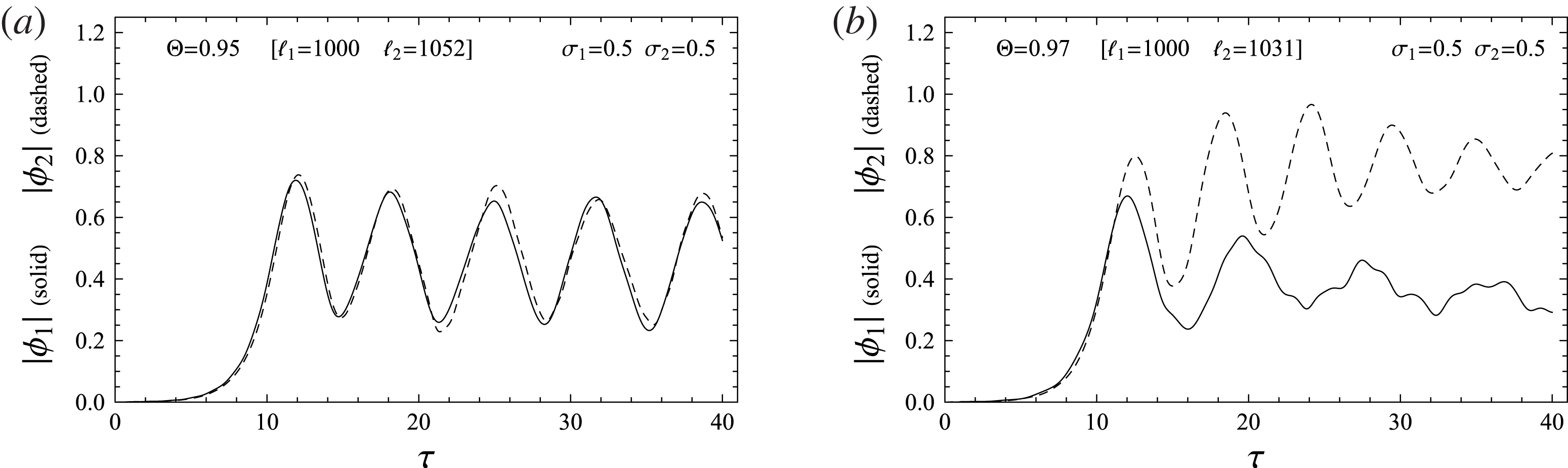
, respectively. In figure 1, we plot the resulting wave amplitude, obtained as a function of time, setting
 ${\it\sigma}_{1}={\it\sigma}_{2}=0.5$
in order give equal weight to the two beams. As initial conditions, we consider the fields of order
 $O(10^{-2})$
and the sheets randomly distributed in
 $0<\bar{{\it\xi}}_{1,2}(0)<2{\rm\pi}$
, while the velocities at
 ${\it\tau}=0$
are
 $\bar{{\it\xi}}_{1}^{\prime }(0)=-\bar{{\it\xi}}_{2}^{\prime }(0)={\rm\pi}(v_{1}-v_{2})/L{\it\omega}_{p}\bar{{\it\eta}}=(1-{\it\Theta})/2\ell _{1}\bar{{\it\eta}}$
. Finally, the values of
 ${\it\beta}_{j}$
from (3.2) are now
 ${\it\beta}_{j}=[\ell _{j}(1+{\it\Theta})/2\ell _{1}-1]/\bar{{\it\eta}}$
, with
 $\ell _{2}=\ell _{1}/{\it\Theta}$
.
Plots of the temporal evolution of
 $|{\it\phi}_{j}|$
determined by the system (3.3). We have set two different values of the parameter
 ${\it\Theta}$
as indicated in the graphs and the simulations are run for
 ${\it\sigma}_{1}={\it\sigma}_{2}$
. The initial conditions and the parameter values are discussed in the text.

From the behaviour of the mode amplitudes, the presence of a threshold value of
 ${\it\Theta}$
clearly emerges, below which the two beams evolve independently generating two well separated single mode profiles. The transition to the interaction regime is anyway rather smooth.
When
 ${\it\Theta}<0.96$
, the generated field profile corresponds to two independent resonant modes. The amplification of both the waves proceeds as in the O’Neil analysis, where the initial exponential instability is followed by periodic oscillations. Furthermore, the instability is proportional to the corresponding
 ${\it\sigma}$
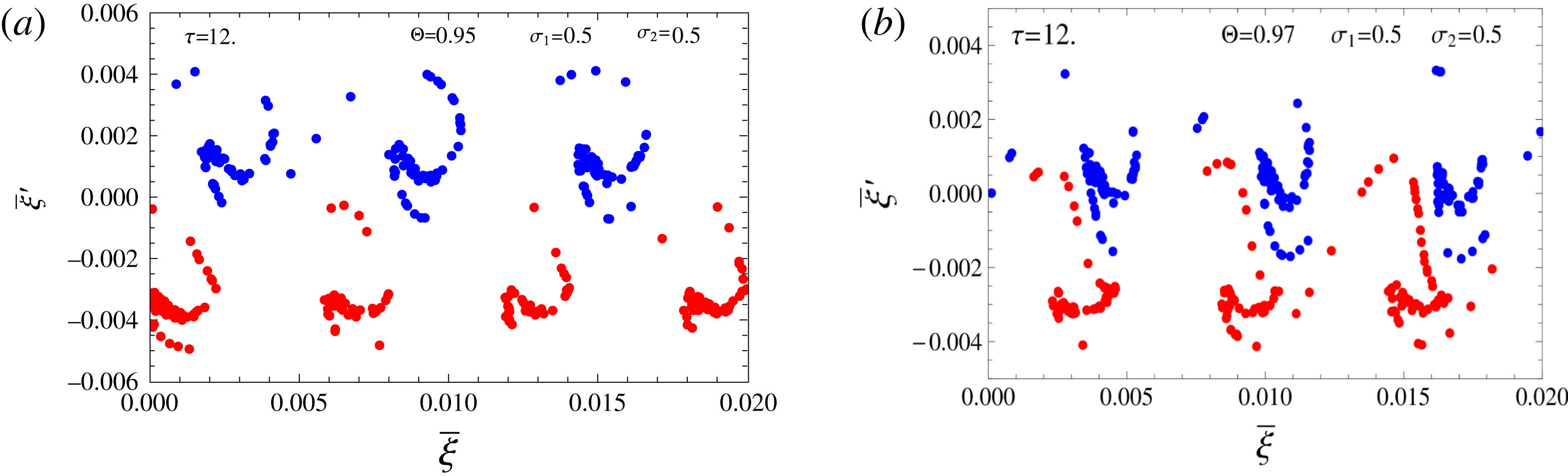
values, consistent with linear theory. The dynamical independence of the beams can be argued also from the left panel of figure 2, where the phase-space is depicted at a fixed time. Coherent with the single wave model, the dynamics of the system leads to the formation of rotating clumps which follow the corresponding Langmuir mode. The number of such coherent structures is related to the wavenumber and we observe
 $\ell _{1}$
(beam 1 in blue) and
 $\ell _{2}$
(beam 2 in red) clumps in the periodicity length
 $L=2{\rm\pi}$
. The synchronized clumps evolve independently and no interference or transport between the two beams occurs. This behaviour has been obtained in all the simulations for
 ${\it\Theta}<0.96$
.
Reduced phase-space
 $(\bar{{\it\xi}},\bar{{\it\xi}}^{\prime })$
snapshots for fixed times (indicate in the graphs). Each point corresponds to a charge sheet labelled by
 $i$
in the system (3.3), the beam 1 (2) is represented in blue (red), the beams have equal densities. We have set
 ${\it\Theta}=0.95$
(a) and
 ${\it\Theta}=0.97$
(b).

When
 ${\it\Theta}\gtrsim 0.96$
, the onset of interaction phenomena between the two beams is clear from figure 1. Analysing the phase-space dynamics in this case (in figure 2
b, we set
 ${\it\Theta}=0.97$
), we observe how during the formation of the rotating clumps, i.e. during the initial exponential evolution of the mode, the charge sheets of the first beam are involved in the dynamics associated to the second one. This yields the evolution of the Langmuir waves described in figure 1 for the same parameter values, where the leading mode is indeed
 ${\it\phi}_{2}$
. Such a mechanism is consistent with the fact that the mode
 ${\it\phi}_{2}$
is excited by the slower beam and can tap energy from the mode
 ${\it\phi}_{1}$
via wave–particle interactions with the faster beam particles.
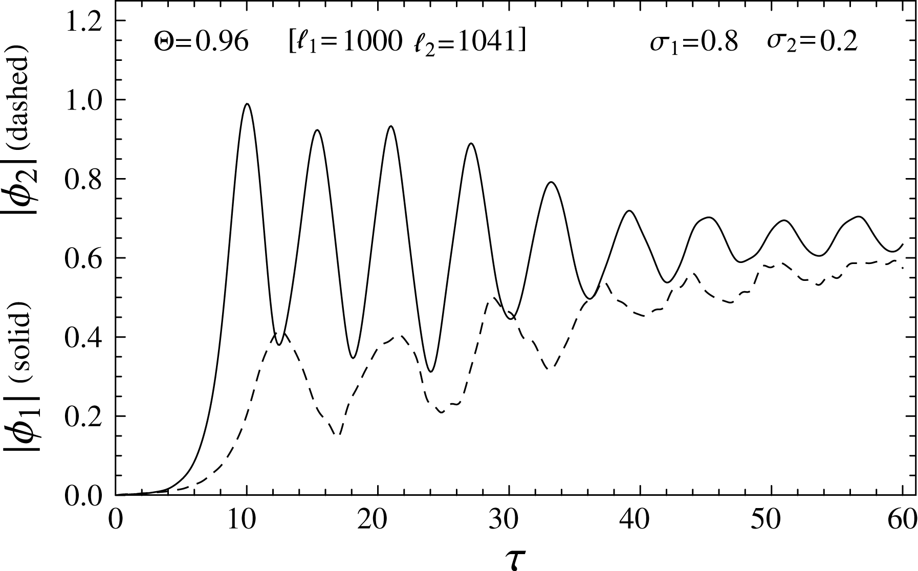
Interaction phenomena are evident also in the case of different values of the beam densities. In this respect, it is worth noting that a peculiar feature emerges near the threshold
 ${\it\Theta}$
-value when
 ${\it\sigma}_{1}$
is significantly greater than
 ${\it\sigma}_{2}$
, see figure 3. The larger density of the first beam forces the second mode to evolve differently compared to the equal density case. In particular, the weaker mode
 ${\it\phi}_{2}$
is increased by the presence of the other one, again, because of energy transfer mediated by wave–particle interactions. This mechanism is analogous but opposite to the ‘surf’ phenomenon occurring in plasma acceleration processes (Keinigs & Jones Reference Keinigs and Jones1987; Esarey et al.
Reference Esarey, Sprangle, Krall and Ting1996; Litos et al.
Reference Litos, Adli, An, Clarke, Clayton, Corde, Delahaye, England, Fisher, Frederico, Gessner, Green, Hogan, Joshi, Lu, Marsh, Mori, Muggli, Vafaei-Najafabadi, Walz, White, Wu, Yakimenko and Yocky2014). Specifically, when the second beam velocity
 $v_{2}$
is close to the enhanced Langmuir mode phase velocity,
 ${\it\phi}_{2}$
continues to tap energy from the faster beam. Thus, the weaker/slower mode can grow at the expense of the stronger/faster mode, via power transfer mediated by wave–particle interactions. In order to clarify the mechanism underlying this phenomenon, we can plot the power exchanged between each beam and individual modes, in the case under consideration (
 ${\it\Theta}=0.96$
and
 ${\it\sigma}_{1}=0.8$
,
 ${\it\sigma}_{2}=0.2$
). For the beam
 $a$
and the mode
 $j$
the dimensionless power can be written using the scaled variables in the reference frame of the average beam speed as:
 $$\begin{eqnarray}P_{a}^{(j)}=\mathop{\sum }_{i=1}^{N_{a}}\left(\text{i}\ell _{j}^{-1}{\it\phi}_{j}\text{e}^{\text{i}\ell _{j}\bar{{\it\xi}}_{ai}+\text{i}{\it\beta}_{j}{\it\tau}}\left(\bar{{\it\xi}}_{ai}^{\prime }+\frac{{\rm\pi}(v_{1}+v_{2})}{{\it\omega}_{p}\bar{{\it\eta}}L}\right)+\text{c.c.}\right).\end{eqnarray}$$
This quantity is plotted in figure 4 as a function of
 ${\it\tau}$
separately for the two modes and with two different time averages, as indicated in the figure, in order to better illustrate the global power transfer features. It is easy to realize from the right-hand panels that, when the ‘anti-surf’ mechanism begins (
 ${\it\tau}\sim 20$
, see figure 3) the power exchanged by the two beams is comparable. Indeed, the particles of the fastest beam transfer energy to the mode
 $\ell _{2}$
and drain energy from the mode
 $\ell _{1}$
. This behaviour of power transfer confirms and clarifies the time evolution of the mode amplitude sketched in figure 3.
Plots of the temporal evolution of
 $|{\it\phi}_{j}|$
by setting
 ${\it\Theta}=0.96$
and
 ${\it\sigma}_{1}=0.8$
,
 ${\it\sigma}_{2}=0.2$
.

Temporal evolution of
 $P_{a}^{(j)}$
((a,c) the mode
 $j=1$
; (b,d) the mode
 $j=2$
) by setting
 ${\it\Theta}=0.96$
and
 ${\it\sigma}_{1}=0.8$
,
 ${\it\sigma}_{2}=0.2$
. The power exchanged by the beam
 $a=1$
(2) is plotted in black (red). In the upper (lower) panels, we have time averaged the power over a step
 ${\rm\Delta}{\it\tau}=2$
(
 ${\rm\Delta}{\it\tau}=4$
) in order to smooth out small rapid oscillations. The transferred energy to the mode
 $\ell _{2}$
from the two beams is comparable, indicating the extraction of power from the mode
 $j=1$
to the mode
 $j=2$
.

We conclude by briefly discussing the limit case for
 ${\it\Theta}$
of order
 $\bar{{\it\eta}}$
. In particular, when
 ${\it\Theta}\gtrsim 0.995$
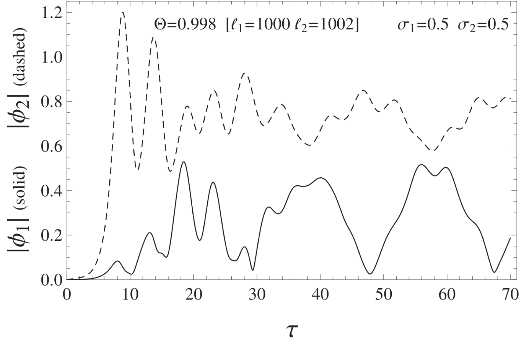
, we observe the onset of a very particular behaviour of the mode nonlinear evolution, as indicated in figure 5 where we have set, as an example,
 ${\it\Theta}=0.998$
. This is due to the fact that the beam instabilities overlap and the resulting dynamics is completely different from the previous cases. As soon as the clumps form, the beam charge sheet interference is strong and the two beams can be effectively treated as a single phase-space structure but in the presence of peculiar time-dependent potentials generated by a fully interacting regime.
Plots of the temporal evolution of
 $|{\it\phi}_{j}|$
by setting
 ${\it\Theta}=0.998$
and
 ${\it\sigma}_{1}=0.5$
,
 ${\it\sigma}_{2}=0.5$
.

3.2. Quasi-degenerate modes
Let us now analyse how, in addition to the two most unstable waves discussed above, the two beam system can excite other nearly degenerate modes, i.e. fluctuations at frequency
 ${\it\omega}_{j}\simeq {\it\omega}_{p}$
implying
 ${\it\epsilon}_{p}\simeq 0$
.
For
 ${\it\Theta}$
over the threshold value for efficient nonlinear beam coupling, these modes correspond to sidebands, defined as
 $k_{j}^{+}=k_{2}+p{\rm\Delta}k$
and
 $k_{j}^{-}=k_{1}-p{\rm\Delta}k$
(where,
 ${\rm\Delta}k=k_{2}-k_{1}$
and
 $p$
is an integer number). These quasi-degenerate modes are responsible for spectral broadening and, possibly, for a cascade phenomenon. To illustrate this process, we now discuss the case
 $p=1$
, considering thus the two sideband modes
 $k_{3}^{+}=2k_{2}-k_{1}$
and
 $k_{3}^{-}=2k_{1}-k_{2}$
. In the reference frame of the average beam speed, the dynamical equations governing the system can be easily constructed generalizing (3.3) for the two additional quasi-degenerate modes. The corresponding mismatch parameters are
 ${\it\beta}_{3}^{+}=[1/{\it\Theta}-{\it\Theta}/2-1/2]/\bar{{\it\eta}}$
,
 ${\it\beta}_{3}^{-}=[{\it\Theta}-1/2{\it\Theta}-1/2]/\bar{{\it\eta}}$
.
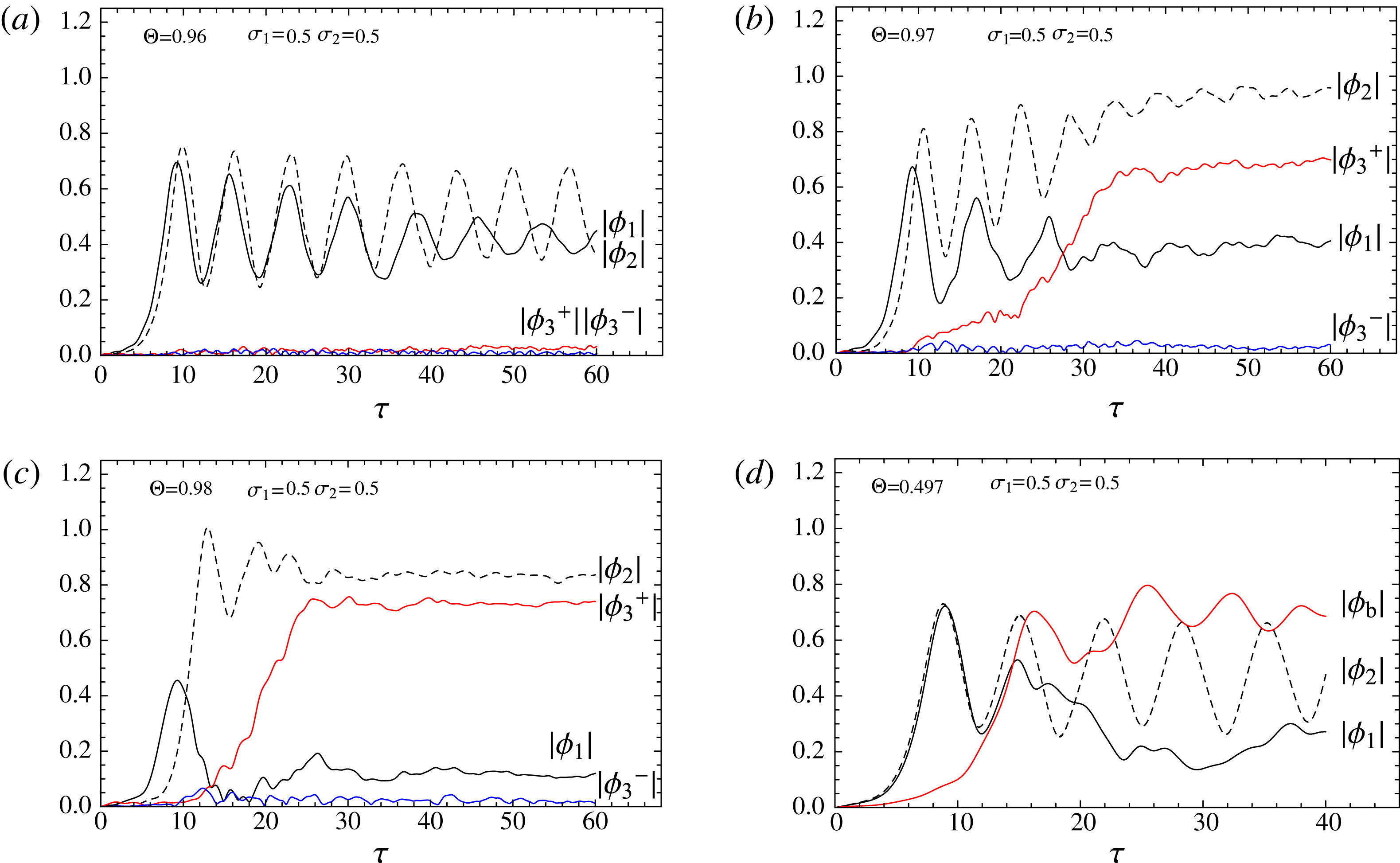
From the first three panels of figure 6, only the
 $k_{3}^{+}$
mode can be excited, while
 $k_{3}^{-}$
does not grow since its resonance condition corresponds to velocities larger than
 $v_{1}$
and, further, it is associated with a negative value of the dielectric function (its frequency is actually slightly smaller than
 ${\it\omega}_{p}$
). It is important to note that the unstable mode at
 $k_{3}^{+}$
saturates at a comparable amplitude to the resonant mode
 ${\it\phi}_{2}$
although saturation is reached at a later time. Meanwhile,
 $k_{3}^{+}$
sideband excitation can occur only above the threshold condition in
 ${\it\Theta}$
for efficient nonlinear beam coupling. In fact, the mechanism for sideband excitation is the same as that for power transfer from faster to slower resonant modes discussed above.
(a–c) Plots of the temporal evolution of
 $|{\it\phi}_{1}|$
,
 $|{\it\phi}_{2}|$
,
 $|{\it\phi}_{3}^{+}|$
and
 $|{\it\phi}_{3}^{-}|$
for different values of
 ${\it\Theta}$
as indicated in the graphs. (d) Plot of the mode
 ${\it\phi}_{b}$
as function of time. For this figure, we set
 ${\it\sigma}_{1}={\it\sigma}_{2}$
and
 $\bar{{\it\eta}}=0.01$
.

Efficient sideband generation can also occur in the case of two independent resonant beam modes, under special limiting conditions. This is the case when
 ${\it\Theta}\rightarrow 1/2^{-}$
; i.e.
 $k_{2}\rightarrow 2k_{1}^{+}$
and the beat mode
 $k_{b}\equiv k_{2}-k_{1}\rightarrow k_{1}^{+}$
. In fact, in this case, illustrated in the right-hand panel of figure 6, the
 $k_{b}$
mode (
 ${\it\phi}_{b}$
in the plot) is quasi-degenerate with the Langmuir frequency
 ${\it\omega}_{p}$
and has a resonance condition at velocities slightly below
 $v_{1}$
. Thus, it must be treated nonlinearly as with the two most unstable modes. As shown in the figure, the saturation level of the quasi-degenerate mode approaches the same value of
 ${\it\phi}_{2}$
saturation, while the evolution of
 ${\it\phi}_{1}$
is significantly altered because
 ${\it\phi}_{b}$
absorbs a relevant part of its energy via nonlinear wave–particle interaction. It can be also demonstrated that
 ${\it\phi}_{b}$
is not efficiently exited as
 ${\it\Theta}\rightarrow 1$
. This fact is consistent with the original problem studied by O’Neil et al. (Reference O’Neil, Winfrey and Malmberg1971), where mode–mode interactions are negligible.
4. Lagrangian Coherent Structures and the transport processes
In this section, we analyse transport processes in order to identify the regions where mixing phenomena are fastest and, in particular, their boundaries that are known as LCS. The LCS technique was introduced by G. Haller in order to generalize intrinsically asymptotic concepts in dynamical systems theory, such as stable and unstable manifolds, to the study of systems over a finite time span
 ${\rm\Delta}{\it\tau}$
. In the same way the separatrix of a pendulum splits the phase-space into two macro regions where initial conditions have different asymptotic behaviour, i.e. rotations and librations, the LCS of the beam–plasma system split the particles into two groups, i.e. recirculating and non-recirculating ones over the finite time span
 ${\rm\Delta}{\it\tau}$
. Without entering into the mathematical details of the definition, following Haller (Reference Haller2015) we state that LCS need to be defined as material lines, i.e. lines advected by the flow, which are locally most repulsive with respect to the nearby ones over the time span
 ${\rm\Delta}{\it\tau}$
. Two initial conditions taken on different sides of an LCS will increase their distance over the time span
 ${\rm\Delta}{\it\tau}$
more than two initial conditions on two sides of any other curve. Therefore they will have, in general, a qualitatively different evolution in the same way that two initial conditions starting on different sides of the stable manifold of a pendulum will increase their distance more than two initial conditions taken on the same side. This leads to the definition of a functional, called repulsion rate, which needs to be maximized on the LCS trough a variational approach (Haller Reference Haller2011; Falessi et al.
Reference Falessi, Pegoraro and Schep2015). This technique has already been used in the computational fluid dynamics community (Haller Reference Haller2001; Shadden et al.
Reference Shadden, Lekien and Marsden2005; Garth et al.
Reference Garth, Gerhardt, Tricoche and Hagen2007; Pascucci et al.
Reference Pascucci, Tricoche, Hagen and Tierny2010; Senatore & Ross Reference Senatore and Ross2011) and, more recently, in plasma physics (Borgogno et al.
Reference Borgogno, Grasso, Pegoraro and Schep2011a
,Reference Borgogno, Grasso, Pegoraro and Schep
b
). An introductory discussion on the proper operational definition of these structures can be found in Falessi et al. (Reference Falessi, Pegoraro and Schep2015). Meanwhile, for a different approach to the characterization of coherent structures, see Leoncini & Zaslavsky (Reference Leoncini and Zaslavsky2002).
4.1. General approach
In the recent review (Haller Reference Haller2015), the author states that an LCS can be sought as an extremizing curve of the FTLE field, i.e. a ridge. Actually, a debate exists in the literature about the proper definition of a ridge. We refer the interested reader to Haller (Reference Haller2015) or to Falessi et al. (Reference Falessi, Pegoraro and Schep2015) for more in-depth discussions of applications of this method in plasma physics. In our analysis, following Haller (Reference Haller2015), we define a ridge of the FTLE field as a curve along which one sees a smaller change in the value of the field than in the direction transverse to it. The resultant contour plot of the FTLE is very peaked and almost constant on nearly 1-D regions. We will identify these structures with the ridges of the FTLE field and, therefore, with the LCS of the system (Voth, Haller & Gollub Reference Voth, Haller and Gollub2002; Kasten et al. Reference Kasten, Petz, Hotz, Hege, Noack and Tadmor2010; Lekien & Ross Reference Lekien and Ross2010; Tang et al. Reference Tang, Mathur, Haller, Hahn and Ruggiero2010; Chian et al. Reference Chian, Rempel, Aulanier, Schmieder, Shadden, Welsch and Yeates2014).
In order to characterize the FTLE fields for a given configuration, the trajectories of several test particles are traced when evolved in the time-dependent potentials
 $\bar{{\it\phi}}(\bar{{\it\xi}},{\it\tau})$
(using the notation of the two beam problem) generated self-consistently by the charge distribution. For a single reference time, the test particles are initialized to sample the whole phase-space of interest (depending on the parameters). The system is composed of an arbitrarily large number of particles and, therefore, we can neglect the contribution of a single test particle in the modification of the potentials, which are treated as assigned for a correspondent beam–plasma simulation. This approximation has already been used in Smith & Pereira (Reference Smith and Pereira1978), Tennyson et al. (Reference Tennyson, Meiss and Morrison1994).
To evaluate the FTLE profile for a fixed time
 ${\it\tau}$
, the test particles are initialized in two phase-space grids of
 $M/2$
particles each and having an initial infinitesimal displacement in the velocity direction. In other words, a test particle located in
 $[\bar{{\it\xi}},\bar{{\it\xi}}^{\prime }]$
has a neighbour initialized in
 $[\bar{{\it\xi}},\bar{{\it\xi}}^{\prime }+{\it\delta}_{{\it\tau}}]$
. With the assigned time-dependent potentials, at a time
 ${\it\tau}+{\rm\Delta}{\it\tau}$
the considered two test particles will be at a distance
 ${\it\delta}_{{\rm\Delta}{\it\tau}}$
in the phase-space and the FTLE value
 ${\it\sigma}$
in the point
 $[\bar{{\it\xi}},\bar{{\it\xi}}^{\prime }]$
is evaluated as (Haller Reference Haller2011)
 $$\begin{eqnarray}{\it\sigma}(\bar{{\it\xi}},\bar{{\it\xi}}^{\prime },{\it\tau},{\rm\Delta}{\it\tau})=\ln ({\it\delta}_{{\rm\Delta}{\it\tau}}/{\it\delta}_{{\it\tau}})/{\rm\Delta}{\it\tau}.\end{eqnarray}$$
When considering a positive time evolution
 ${\rm\Delta}{\it\tau}>0$
, the curves where the FTLE field is peaked define a repulsive transport barrier, while setting
 ${\rm\Delta}{\it\tau}<0$
and evolving the system backward in time they represent an attractive barrier. Approximated 1-D structures which correspond to the LCS can be built by plotting the maximum values of
 ${\it\sigma}(\bar{{\it\xi}},\bar{{\it\xi}}^{\prime },{\it\tau},{\rm\Delta}{\it\tau})$
as extracted from a contour plot. In the analysis of this Section, we have set two grids of
 $250\times 250$
test particles (
 $M=125\,000$
), thus obtaining 62 500 values of the FTLE for each phase-space snapshot. The self-consistent fields
 $\bar{{\it\phi}}({\it\tau})$
have been sampled from the complete Hamiltonian simulation with the proper selected parameters.
4.2. The single wave model
As a first step, we apply the FTLE method to characterize the dynamical system describing the single wave model (O’Neil et al.
Reference O’Neil, Winfrey and Malmberg1971), which can be easily deduced from (2.12) by considering one beam and one mode
 $j=1$
. In Tennyson et al. (Reference Tennyson, Meiss and Morrison1994) and Smith & Pereira (Reference Smith and Pereira1978), the test particle approximation is used for studying the behaviour of the single wave model using dynamical systems techniques. In particular, in the latter, the evolution of the electromagnetic field is modelled with an analytic function while in the former, it is extracted from the numerical simulations as in the present paper. In Tennyson et al. (Reference Tennyson, Meiss and Morrison1994), the periodicity of the asymptotic state of the system is exploited in order to generate a Poincaré section (stroboscopic map) of the motion, i.e. the sampling of the evolution of a particle after each periodic oscillation of the electromagnetic field. The set of points obtained by this procedure, for different initial conditions, can be used to distinguish different kinds of motion: periodic, quasi-periodic or chaotic. In both works mentioned above, a region of non-chaotic motion is present. This region moves, with a periodic behaviour, coherently, i.e. only with slight deformations in its shape. Some of the beam particles will start inside this structure and thus they will be trapped during their entire evolution. This is the mechanism responsible for the formation of the clump in the Hamiltonian system and for the bunching of the particles. This procedure splits the ensemble of trajectories and thus the ensemble of the available particle motions, relying on their asymptotic behaviour. For this reason, this scheme identifies barriers for the transport processes in the system which holds at any time, i.e. curves which cannot be crossed by the particles during their motion. In the most general aperiodic case however, such structures do not exist because every trajectory could in principle be chaotic and, furthermore, it is not clear how the stroboscopic map technique can be used for studying the single wave model during linear growth.
In this work, we are interested in studying the system during the onset of the instability. For this reason, the periodicity of the electromagnetic potential is generally lost. Using the FTLE method in order to identify the shapes of the LCS can nonetheless split the phase space into different regions based on the behaviour of the trajectories over a finite period of time. These structures, which are characterized by a peaked FTLE field, approximate the unstable (stable) manifolds of the dynamical system and characterize the transport through the lobes dynamics (Malhotra & Wiggins Reference Malhotra and Wiggins1998).
The two parameters that characterize the FTLE values are
 ${\it\tau}$
and
 ${\rm\Delta}{\it\tau}$
. The time evolution of the LCS is identified by the first, while the second determines how refined the LCS will be. By choosing an increasingly longer integration time
 ${\rm\Delta}{\it\tau}$
, the obtained LCS acquire more intricate structures because of an increasingly better approximation to the homoclinic tangle. This kind of dynamics have been studied by Malhotra & Wiggins (Reference Malhotra and Wiggins1998) and leads to the splitting of the phase-space into macro-regions which exchange a relatively small amount of particles over a characteristic time scale. The characterization of the detailed shape of the stable and unstable manifolds, which can be achieved trough an FTLE plot with long
 ${\rm\Delta}{\it\tau}$
, gives insights into the time asymptotic transport processes. The shape of the LCS obtained with smaller values of
 ${\rm\Delta}{\it\tau}$
, meanwhile, highlights the boundaries of the macro-regions with small transport among them.
Here, we are interested in the shape and the location of these regions and thus the integration time is fixed at
 ${\rm\Delta}{\it\tau}=4$
after a number of tests, obtaining a simple, closed region as shown in the left panel of figure 7, where we have over-plotted the beam-particle positions to the LCS. The effect discussed above of increasing
 ${\rm\Delta}{\it\tau}$
can be deduced by comparing with the middle panel. Increasing the value of
 ${\it\tau}$
, we get the position of the LCS at different instants and, therefore, the motion of the ‘finite time’ transport barriers. From these plots it can be argued that, during the onset of the instability, most of the beam particles are trapped inside the central region delimited by the LCS and, therefore, they recirculate and start forming the clump.
Overlay of the phase-space snapshots (black or red points) and the LCS (thick lines) determined as the peaks of the FTLE fields extracted from a corresponding contour plot built using (4.1). (a) LCS for the single wave model for
 ${\it\tau}=12.5$
and
 ${\rm\Delta}{\it\tau}=4$
. (b) LCS for
 ${\it\tau}=11$
and
 ${\rm\Delta}{\it\tau}=10$
(in this plot, the beam particles are highlighted in red). (c) LCS in the late evolution for
 ${\it\tau}=156$
and
 ${\rm\Delta}{\it\tau}=4$
.

In order to make a comparison with Tennyson et al. (Reference Tennyson, Meiss and Morrison1994), we can calculate the LCS for larger values of
 ${\it\tau}$
, when the electromagnetic potential oscillates periodically. We obtain the plot on the right-hand panel of figure 7, where the transport barriers are splitting the chaotic region into two different areas having qualitatively different motions on a short time scale. The points outside the central ‘eye’ have a motion similar to rotations in a pendulum, while the points inside the ‘eye’ resemble librations. In contrast to an unperturbed pendulum, the points may start undergoing rotational motion and later, undergo librational motion and vice-versa. However, this transition has a typical ‘long’ time scale and, if we look at the transport processes which happen over a shorter time, the two different kinds of trajectories do not mix. For this reason the LCS may be regarded as finite time transport barriers.
4.3. The two wave model
Let us now analyse the transport processes in the two beam system using the same methodology introduced above. In figure 8, we plot the LCS and the particle phase-space at different values of
 ${\it\Theta}$
during the onset of the instability for
 ${\it\tau}=11.6$
and
 ${\rm\Delta}{\it\tau}=5$
.
Overlay of the phase-space snapshots (blue and red points for the beam 1 and 2, respectively) and the LCS (thick lines) defined through the contour plot peaks of the FTLE fields evaluated by (4.1). The beam densities are set as
 ${\it\sigma}_{1}={\it\sigma}_{2}=0.5$
and
 ${\it\tau}=11.6$
and
 ${\rm\Delta}{\it\tau}=5$
. The different values of the beam initial velocity ratio (
 ${\it\Theta}$
) are indicated in the graphs.

Considering the different coloured particles initially belonging to different beams, it can be argued that they form a single phase-space structure for sufficiently small values of
 $1-{\it\Theta}$
. In the first plot, two eye-shaped regions delimited by the LCS clearly emerge. Correspondingly, the particles of the different beams do not mix. The shape of the LCS becomes increasingly complicated as
 ${\it\Theta}\rightarrow 1$
. In the most general case, the LCS do not divide the phase-space into separate regions and, correspondingly, the particles of different beams can mix into a single structure. Therefore, the mixing process is greatly enhanced when LCS belonging to different beams intersect; and they cannot be considered as finite time transport barriers between separate phase-space regions. We refer to
 ${\it\Theta}_{\mathit{crit}}$
as the smallest value of
 ${\it\Theta}$
compatible with the merging of the beams and give an estimate of such a threshold by increasing
 ${\it\Theta}$
until two LCS belonging to different beams intersect. From the plots in figure 8, we obtain
 ${\it\Theta}_{\mathit{crit}}$
between 0.96 and 0.97. For different beam densities, this method yields similar values of
 ${\it\Theta}_{\mathit{crit}}$
. In the work Borgogno et al. (Reference Borgogno, Grasso, Pegoraro and Schep2008), a similar analysis was carried out in order to study the transition from local to global chaos in the magnetic field lines of a reconnecting current layer.
We conclude this Section with a derivation of
 ${\it\Theta}_{\mathit{crit}}$
using the Chirikov criterion. Following O’Neil et al. (Reference O’Neil, Winfrey and Malmberg1971), the velocity spread of particles trapped by a single saturated beam mode is
 ${\rm\Delta}v_{j}=\sqrt{2{\it\phi}_{j}}\,\bar{{\it\eta}}$
. The Chirikov parameter
 $S$
is thus defined by the ratio between the resonance width and the resonance separation of the two beams with initial velocity
 $v_{1}$
and
 $v_{2}$
(i.e.
 $(v_{1}-v_{2})/v_{1}$
). It can then be written as
 $$\begin{eqnarray}S=\frac{2{\rm\Delta}v_{j}}{(v_{1}-v_{2})/v_{1}}=2\frac{\sqrt{2{\it\phi}_{j}}\bar{{\it\eta}}}{1-{\it\Theta}}.\end{eqnarray}$$
By the Chirikov criterion, two resonances overlap if
 $S>1$
; therefore, in the saturation regime (i.e.
 ${\it\phi}_{j}\simeq 1$
), we obtain
 ${\it\Theta}_{\mathit{crit}}\sim 0.97$
, consistent with the previous analysis based on the LCS (considering that
 $\bar{{\it\eta}}$
is fixed as 0.01). We note that, even if the definition of LCS we have used is not rigorous nor unique, their shape is a posteriori consistent with particle dynamics and with the ensuing transport processes. The main advantage of using the LCS technique in studying transport processes between multiple resonant beams is that they can be calculated when the system is not near the saturated regime; thus, also, when the Chirikov criterion cannot be straightforwardly applied.
5. Concluding remarks
In this work, we have proposed to investigate the 1-D bump-on-tail problem in terms of
 $n$
cold beams injected in a cold background plasma behaving as a linear dielectric medium; and
 $m\geqslant n$
self-consistently coupled nonlinear oscillators, mimicking the features of a warm fast particle distribution interacting with a spectrum of resonantly excited Langmuir waves. The use of the Hamiltonian formulation addressed in this work provides a convenient representation of the beam–plasma interaction and of ensuing transport processes at the disparate time and velocity scales underlying the complex behaviours of this system.
Specializing the model to two supra-thermal beams, we have determined the threshold ratio between the initial beam velocities for which the two corresponding instabilities mutually interact instead of remaining separate growing modes. Such a value has been found to be
 ${\sim}0.96$
for the present simulation parameters, and is consistent with the estimates provided in Levin et al. (Reference Levin, Lyubarskiǐ, Onishchenko, Shapiro and Shevchenko1972) for a supra-thermal hot beam as well as with the Chirikov criterion. Above the threshold, the phase-space analysis of the particle motion clearly shows that transport appears as an exchange of particles between the two beams.
Furthermore, we have discussed the role of other quasi-degenerate modes, with particular attention to sideband modes. More specifically, we have shown that such additional modes may nonlinearly saturate at almost the same level reached by the most unstable waves. This fact suggests that the long time scale evolution of the multi-beam system would be significantly affected by nonlinear sideband generation; and the same would hold for EP transport.
In the last part of the paper, we have investigated the onset of transport in the velocity space in terms of finite time transport barriers defined by the LCS. The critical threshold for transport onset has been analysed in terms of the LCS of the system defined trough the FTLE field. The resulting critical value for the beam initial velocity ratio coincides with the Chirikov criterion and the direct inspection of particle motion in phase-space; providing a very meaningful test of validity for the LCS technique in characterizing the phase-space dynamics.
Our analysis provides a qualitative and quantitative investigation framework for phase-space transport processes in the beam–plasma system. The advantage in using the present paradigm stands in the direct and very general characterization of the phase-space morphology. This leads to the definition of proper characteristic time and velocity scales related with spectral features and wave–particle resonances, together with the characterization of the diffusion coefficient in the quasi-linear limit expected for a large number of modes and a sufficiently broad spectrum.
Acknowledgements
This work has been carried out within the framework of the EUROfusion Consortium and has received funding from the Euratom research and training programme 2014–2018 under grant agreement no. 633053. The views and opinions expressed herein do not necessarily reflect those of the European Commission.