1. Introduction
The applications of small-scale vehicles, such as micro air vehicles (MAVs) for Mars exploration (Shrestha et al. Reference Shrestha, Benedict, Hrishikeshavan and Chopra2016), unmanned air vehicles (UAVs) for agriculture monitoring (Floreano & Wood Reference Floreano and Wood2015) and autonomous underwater vehicles (AUVs) for maritime security (Xu, Baglietto & Brizzolara Reference Xu, Baglietto and Brizzolara2018), have proliferated in recent years. Low-Reynolds-number flows are often encountered in these applications with airfoil-chord Reynolds number Rec < 5 × 10⁵ (Lissaman Reference Lissaman1983; Mueller & Delaurier Reference Mueller and Delaurier2003). Because of the low Rec, the laminar boundary layer over the suction side of an airfoil is heavily susceptible to separation. The separated boundary layer is highly unstable and could dramatically affect the aerodynamic efficiency by undergoing a laminar-to-turbulent transition (Di Luca et al. Reference Di Luca, Mintchev, Su, Shaw and Breuer2020). Aiming at aerodynamic optimization, this separation-induced transition has been extensively explored by the academic community (Burgmann, Dannemann & Schröder Reference Burgmann, Dannemann and Schröder2008; Hain et al. Reference Hain, Kähler and Radespiel2009; Marxen et al. Reference Marxen, Lang, Rist, Levin and Henningson2009; Jones et al. Reference Jones, Sandberg and Sandham2010; Marxen & Henningson Reference Marxen and Henningson2011; Boutilier & Yarusevych Reference Boutilier and Yarusevych2012b; Robinet Reference Robinet2013; Serna & Lázaro Reference Serna and Lázaro2014, Reference Serna and Lázaro2015; Kurelek, Lambert & Yarusevych Reference Kurelek, Lambert and Yarusevych2016; Yarusevych & Kotsonis Reference Yarusevych and Kotsonis2017; Kurelek, Kotsonis & Yarusevych Reference Kurelek, Kotsonis and Yarusevych2018; Hosseinverdi & Fasel Reference Hosseinverdi and Fasel2019).
As a traditional high-lift configuration, a multi-element airfoil can postpone the stall and enhance the maximum lift coefficient at high Reynolds numbers (Prandtl Reference Prandtl1904; Weyl Reference Weyl1945; Smith Reference Smith1975; Van Dam Reference Van Dam2002). It is desirable for low-Reynolds-number vehicles to benefit from adopting this configuration after necessary redesigns and optimizations. Correspondingly, the low-Reynolds-number flows over multi-element airfoils should be deeply understood in flow physics to realize this conception. As the main contributor to lift generation (Pascioni & Cattafesta Reference Pascioni and Cattafesta2018), the main element inherently bears the disturbance of slat wakes (Squire Reference Squire1989). The slat wake can even merge with the original boundary layer of the main element and finally lead to a confluent boundary layer (Thomas, Nelson & Liu Reference Thomas, Nelson and Liu2000). In contrast to the separation-induced transition mentioned above, the transition of the confluent boundary layer is strongly affected by the slat wake and remains an open issue. The current work is therefore focused on this type of wake-induced transition at low Reynolds numbers to benefit the future design of low-Reynolds-number vehicles.
Because of the geometrical complexity of multi-element airfoils, the wake-induced transition is normally explored with a simplified configuration. A circular cylinder and a flat plate are used to generate the wake and laminar boundary layer, respectively. In the pioneering hot-wire measurements of Kyriakides et al. (Reference Kyriakides, Kastrinakis, Nychas and Goulas1999), the circular cylinder was placed upstream of the leading edge of the flat plate. The quadrant-splitting analyses and ensemble averaging of hot-wire signals revealed that the wake vortex with negative vorticity induced a spanwise secondary vortex with positive vorticity in the boundary layer. These secondary vortices were treated as the precursors of transition. However, with a configuration similar to that of Kyriakides et al. (Reference Kyriakides, Kastrinakis, Nychas and Goulas1999), Ovchinnikov, Piomelli & Choudhari (Reference Ovchinnikov, Piomelli and Choudhari2006) revealed a different transition routine by numerical simulations. The deformed wake vortices (due to three-dimensional instability) injected wake disturbances into the boundary layer, leading to streaky structures. These streaky structures were the precursors of transition, similar to the scenario of the free-stream-turbulence-induced (FST-induced) transition (Matsubara & Alfredsson Reference Matsubara and Alfredsson2001).
The different transition routines mentioned above motivated the experimental investigations of Pan et al. (Reference Pan, Wang, Zhang and Feng2008). With hydrogen bubble visualizations, Pan et al. (Reference Pan, Wang, Zhang and Feng2008) clearly captured spanwise secondary vortices within the boundary layer, as the direct response to wake vortices. As the precursors of transition, these secondary vortices deformed to generate Λ vortices and further led to hairpin vortex packets at the late stage of the transitional boundary layer. These hairpin vortex packets and associated streaky structures contributed to a self-sustaining turbulent boundary layer. The transition routine of Pan et al. (Reference Pan, Wang, Zhang and Feng2008) was further verified by the quantitative particle image velocimetry (PIV) measurements of Mandal & Dey (Reference Mandal and Dey2011). This PIV investigation also suggested similarities between the wake-induced transition and the FST-induced transition at the late stage.
Notably, all the wake-induced transitions mentioned above occur slightly downstream of the leading edges of flat plates. Pan et al. (Reference Pan, Wang, Zhang and Feng2008) argued that the complex leading-edge receptivity (Nagarajan, Lele & Ferziger Reference Nagarajan, Lele and Ferziger2007; Schrader et al. Reference Schrader, Brandt, Mavriplis and Henningson2010) could be responsible for the different transition routines between Kyriakides et al. (Reference Kyriakides, Kastrinakis, Nychas and Goulas1999) and Ovchinnikov, Piomelli & Choudhari (Reference Ovchinnikov, Piomelli and Choudhari2006). To avoid this leading-edge receptivity, He, Wang & Pan (Reference He, Wang and Pan2013) conducted an experimental investigation with a circular cylinder placed downstream of the flat plate's leading edge. Spanwise secondary vortices still occurred within the boundary layer. The wake disturbances, which had the same frequency as that of the shedding of wake vortices, survived the shear-sheltering effect (Durbin & Wu Reference Durbin and Wu2007) and penetrated the boundary layer. The exponential growth of these disturbances resulted in secondary vortices.
Subsequently, He et al. (Reference He, Pan, Feng, Gao and Wang2016) further tracked the Lagrangian coherent structures throughout the transition process. At the intermediate stage of transition, the deformed secondary vortices had the same spanwise wavelength as that of the mode-A instability of the cylinder wake (Williamson Reference Williamson1996). Therefore, they speculated that disturbances in the cylinder wake could trigger the three-dimensional destabilization of spanwise secondary vortices.
In summary, great progress has been made in the wake-induced transition with a simplified configuration. However, the wake-induced transition scenario with a multi-element airfoil still requires further investigation. In addition, how wake disturbances affect the three-dimensional destabilization of secondary vortices also needs further exploration.
The wake–shear layer interactions over a 30P30N multi-element airfoil have been explored within the low-Reynolds-number range of 8.32 × 10³ ≤ Rec ≤ 3.05 × 10⁴ (Wang et al. Reference Wang, Feng, Wang and Li2018a,Reference Wang, Wang and Kimb). Wang et al. (Reference Wang, Feng, Wang and Li2018a) found that the boundary of the slat cove bubble provided a virtual curved wall for centrifugal instability, leading to Görtler vortices (streamwise vortices) in the slat wake (Rec = 8.32 × 10³ and α = 2°–12°). These Görtler vortices strongly affected the leading-edge separated shear layer of the main element by triggering streamwise streaks inside it. Subsequently, Wang et al. (Reference Wang, Wang and Kim2018b) explored the effects of Reynolds number on the wake–shear layer interactions over the front part of the main element (α = 4°). Two types of wake–shear layer interactions, divided by a critical interval of 1.27 × 10⁴ < Rec < 1.38 × 10⁴, were captured within the Rec range of 9.3 × 10³ to 3.05 × 10⁴. When Rec ≤ 1.27 × 10⁴, the Görtler vortices in the slat wake could still trigger streamwise streaks in the leading-edge separated shear layer of the main element. When Rec ≥ 1.38 × 10⁴, the rollups of the slat cusp shear layer and their following three-dimensional deformations resulted in the coexistence of spanwise and streamwise vortices in the slat wake. The spanwise wake vortices triggered spanwise secondary vortices above the main element, similar to the scenario of a simplified circular cylinder–flat plate configuration. However, two secondary vortices (denoted as double-secondary vortices) were simultaneously triggered by one wake vortex, in contrast to the single-secondary vortex with a simplified configuration. It was found that the wake disturbances of the fundamental frequency and harmonics simultaneously penetrated the boundary layer of the main element and led to double-secondary vortices.
Although progress has been made in the wake–shear layer interactions over a 30P30N multi-element airfoil, these previous investigations were primarily focused on the flow physics around the leading edge of the main element. Accordingly, how the slat wake affects the downstream evolution of the boundary layer above the main element has not been investigated in detail, and therefore is the focus of the current work. Inspired by the wake-induced transition with a simplified circular cylinder–flat plate configuration (Kyriakides et al. Reference Kyriakides, Kastrinakis, Nychas and Goulas1999; Ovchinnikov et al. Reference Ovchinnikov, Piomelli and Choudhari2006; Pan et al. Reference Pan, Wang, Zhang and Feng2008; Mandal & Dey Reference Mandal and Dey2011; He et al. Reference He, Wang and Pan2013; He et al. Reference He, Pan, Feng, Gao and Wang2016), whether slat-wake-triggered double-secondary vortices play an important role in the transitional confluent boundary layer above the main element will be particularly discussed in the present work, which, to the best of our knowledge, is the first of its kind.
In the current study, the slat-wake-induced transition over the main element of the 30P30N airfoil is investigated with a fixed α of 4° at low Reynolds numbers ( $Re_c=1.38 \times 10^{4}{-}3.05\times10^{4}$) using time-resolved particle image velocimetry (TR-PIV) and hydrogen bubble visualization. The uniqueness of this study lies in the reported laminar-to-turbulent transition routine over a geometry of such relevance to aerospace engineering practice. The effects of slat-wake-triggered double-secondary vortices on the entire transition process are particularly highlighted. Furthermore, two mechanisms are proposed to characterize how the disturbances in the slat wake affect the three-dimensional destabilization of secondary vortices. It is hoped that the flow physics behind this transition routine can promote a deeper understanding of low-Reynolds-number flows over multi-element airfoils. The paper is structured as follows. The experimental setup and post-processing tools are first presented in § 2; the statistical characteristics of the mean flow throughout the transition process are then provided in § 3; the dynamics of coherent structures are subsequently discussed in § 4; and the conclusion is finally drawn in § 5.
2. Experimental methodology
2.1. Experimental set-up
The experiments were performed in the water tunnel of the Institute of Fluid Mechanics at the Beijing University of Aeronautics and Astronautics. The tunnel test section is 600 mm × 600 mm × 3000 mm (height × width × length). More details of this water tunnel can be found in Wang et al. (Reference Wang, Feng, Wang and Li2018a) and Wang et al. (Reference Wang, Wang and Kim2018b). The measurements are conducted using an aluminum 30P30N multi-element airfoil with a stowed chord length (c) and span of 150 and 500 mm, respectively. The aspect ratio of 3.33 (Jenkins, Khorrami & Choudhari Reference Jenkins, Khorrami and Choudhari2004; Pascioni & Cattafesta Reference Pascioni and Cattafesta2018) and the circular endplates at two sides of the airfoil (Boutilier & Yarusevych Reference Boutilier and Yarusevych2012a) guarantee a quasi-two-dimensional mean flow around the middle region of the airfoil (Wang et al. Reference Wang, Wang and Kim2018b). More details of the model design for the current 30P30N airfoil can be found in Wang et al. (Reference Wang, Feng, Wang and Li2018a) and Wang et al. (Reference Wang, Wang and Kim2018b). All tests are performed at an angle of attack (α) of 4°. The chord Reynolds number (Rec) varies from 1.38 × 10⁴ to 3.05 × 10⁴, and the related free-stream velocity (U∞) varies from 92 to 204 mm s−1. To focus on the confluent boundary layer above the main element, the origin of coordinate system O (figure 1) is located at the leading edge of the main element (α = 4°); and X and Y denote the streamwise and vertical directions, respectively. As shown in figure 1, the slat has an inevitable blunt trailing edge (with a thickness smaller than 0.5 mm) for the feasibility of manufacturing. This blunt trailing edge could lead to potential von Kármán vortex streets. However, these potential von Kármán vortex streets are too tiny to be captured by the current measurements. In contrast to the strong wake disturbances generated by the shed vortices of the slat cusp shear layer, these tiny von Kármán vortex streets have a negligible influence on the current wake-induced transition.
Side view of PIV measurements. PIV1 and PIV2 focus on the flows around the gap region and the centre part of the main element, respectively. The black boxes denote the fields of view of PIV1 and PIV2.

2.1.1. Particle image velocimetry
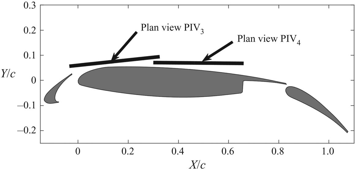
Two-dimensional TR-PIV is used to measure the confluent boundary layer above the main element. In contrast to the single field of view (FOV) used in Wang et al. (Reference Wang, Wang and Kim2018b), four FOVs are designed to provide the side view and plan view properties of the confluent boundary layer (PIV1 and PIV2 in figure 1; PIV3 and PIV4 in figure 2). The PIV system comprises two semiconductor continuous lasers (8 W, 532 nm) for laser sheets and one Photron FASTCAM SA2 high-speed complementary metal oxide semiconductor (CMOS) camera (equipped with a TAMRON lens of 90 mm focal length) for image recording. The shutter time of the CMOS camera equals 1/fs, where fs is the sampling frequency of the CMOS camera. Two vertical laser sheets (thickness of ~1 mm) and the CMOS camera are combined to investigate the flow around the gap region (PIV1 in figure 1). The formation and destabilization of slat-wake-triggered double-secondary vortices will be captured in PIV1. The PIV images are recorded with a sensor resolution of 1536 pixels × 1184 pixels and a magnification of 0.035 mm pixel−1. The related fs varies from 360 to 800 Hz with increasing Rec. The CMOS camera is co-operated with a vertical laser sheet (thickness of ~1 mm) to investigate the turbulent boundary layer around the centre part of the main element (denoted as PIV2 in figure 1). A sensor resolution of 2048 pixels × 864 pixels and a magnification of 0.036 mm pixel−1 are used for the image recording. The related fs still varies from 360 to 800 Hz with increasing Rec. Aiming at the complex three-dimensional effects of the slat wake on the boundary layer over the main element, plan view PIV3 is used to extract the spanwise information of the slat wake and the slat-wake-triggered double-secondary vortices in the boundary layer (figure 2). The inclined laser sheet (thickness of ~1 mm) is designed to simultaneously contain the dominant flow structures pertaining to the slat wake and the slat-wake-triggered double-secondary vortices, with the aid of hydrogen bubble visualization. Notably, the expected results are robust for the locations of the laser sheet to a certain extent, as long as the targeted flow structures are captured in PIV3. The CMOS camera records images with a sensor resolution of 2048 pixels × 1472 pixels and a magnification of 0.038 mm pixel−1. With increasing Rec, the related fs varies from 400 to 960 Hz. Similarly, plan view PIV4 is used to extract spanwise information of the boundary layer above the centre part of the main element (figure 2). Based on the variation in Rec, the CMOS camera samples images with frequencies varying from 300 to 720 Hz. The sensor resolution and the magnification are fixed as 1520 pixels × 1120 pixels and 0.048 mm pixel−1, respectively.
Plan view of PIV measurements. The black lines denote the laser sheets of PIV3 and PIV4.

The final velocity fields are calculated by the multi-pass iterative Lucas–Kanade algorithm (MILK algorithm). The detailed algorithm can be found in Champagnat et al. (Reference Champagnat, Plyer, Le Besnerais, Leclaire, Davoust and Le Sant2011) and Pan et al. (Reference Pan, Xue, Xu, Wang and Wei2015). The ability of this algorithm to provide dense velocity fields of the current 30P30N airfoil with relatively fewer outliers has been validated (Wang et al. Reference Wang, Feng, Wang and Li2018a,Reference Wang, Wang and Kimb). The final interrogation window and the overlap are fixed as 32 pixels × 32 pixels and 75 %, respectively, for all the PIV measurements in the current work. At least 12 585 PIV snapshots are collected for the convergence of statistical estimates. Following the strategies of Qu et al. (Reference Qu, Wang, Feng and He2019), the instantaneous velocity uncertainties relative to the free-stream velocities in all PIV measurements are estimated to be less than 1.8 %. For the statistical analyses in PIV1 and PIV2, the uncertainties of the mean resultant velocity and two-dimensional total kinetic energy are expected to be less than 0.2 % × U∞ and 0.05 % ×  $U_\infty ^2$, respectively. The normalized uncertainty (by dividing U∞/c) of the quasi-vertical vorticity in PIV3 is estimated to be less than 5.2. Notably, the nearest resolved PIV data are approximately 0.5 mm (equal to half of the side length of an interrogation window) from the airfoil surface (PIV1 and PIV2). The wall substantially affects the PIV measurements below this height (Qu et al. Reference Qu, Wang, Feng and He2019). However, the focused flow structures of the current work all reside above this height and therefore are resolved by PIV measurements.
2.1.2. Hydrogen bubble flow visualization
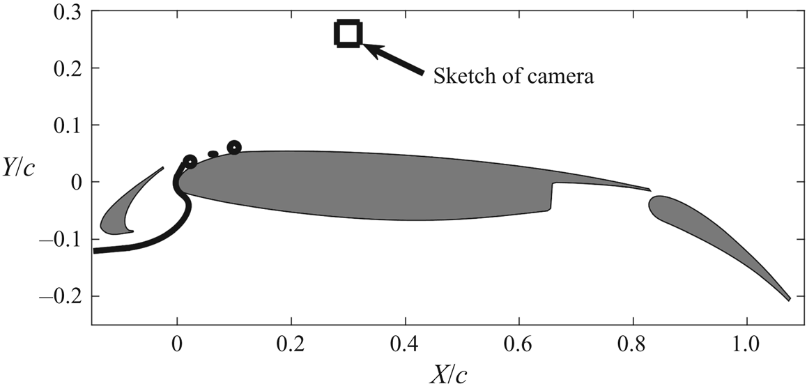
The hydrogen bubble flow visualization in the current work follows the design of previous work (Wang et al. Reference Wang, Feng, Wang and Li2018a,Reference Wang, Wang and Kimb). The horizontal hydrogen bubble curtain emitted from a platinum filament with a diameter of 20 μm strikes the forward stagnation point of the main element and further visualizes the flow structures within the boundary layer of this element (figure 3). The continuous laser and the CMOS camera in PIV measurements are again used for volume illumination and image recording, respectively. In contrast to the limited FOV in Wang et al. (Reference Wang, Wang and Kim2018b), the current FOV could contain most of the main element, enabling the tracking of flow patterns from the initial laminar stage to the late transitional stage.
Plan view of hydrogen bubble visualization. The horizontal hydrogen bubble curtain is designed to strike the forward stagnation point of the main element and further visualizes the flow structures within the boundary layer of the main element. The distance between the camera and airfoil is longer than indicated by the current sketch.

2.2. Post-processing tools
The dynamics of coherent structures throughout the transition process will be demonstrated with the co-operation of several advanced post-processing tools. An overview of these tools is briefly provided here.
2.2.1. Visualization of Lagrangian coherent structures
The finite-time Lyapunov exponents (FTLEs) method (Haller & Yuan Reference Haller and Yuan2000; Haller Reference Haller2001; Shadden, Dabiri & Marsden Reference Shadden, Dabiri and Marsden2006; Green, Rowley & Haller Reference Green, Rowley and Haller2007; Shadden, Astorino & Gerbeau Reference Shadden, Astorino and Gerbeau2010) and virtual dye visualization (VDV) (He et al. Reference He, Wang, Pan, Feng, Gao and Rinoshika2017; Wang et al. Reference Wang, Gao, Wei and Wang2017) can extract Lagrangian coherent structures (LCSs) from complex flows based on tracking fluid particle trajectories. The fluid particle trajectories are characterized by a flow map  $\phi _{{t_0}}^{{t_0} + {t_1}}$ (Shadden, Lekien & Marsden Reference Shadden, Lekien and Marsden2005) and calculated from the discrete PIV velocity data (Jensen, Pedersen & Wood Reference Jensen, Pedersen and Wood2003; He et al. Reference He, Pan, Feng, Gao and Wang2016):
 \begin{equation}\phi _{{t_0}}^{{t_0} + {t_1}}:\boldsymbol{x}({t_0}) \to \boldsymbol{x}({t_0} + {t_1}),\end{equation}
where  $\boldsymbol{x}({t_0})$ and
 $\boldsymbol{x}({t_0} + {t_1})$ denote the positions of fluid particles at
 ${t_0}$ and
 ${t_0} + {t_1}$, respectively. The FTLEs are defined as the exponential growth rate of nearby fluid particle trajectories over the finite time interval
 ${t_1}$ (Haller Reference Haller2001; Shadden et al. Reference Shadden, Dabiri and Marsden2006; Shadden et al. Reference Shadden, Katija, Rosenfeld, Marsden and Dabiri2007):
 \begin{gather}\textrm{FTLE}(\boldsymbol{x},{t_0},{t_1}) = \frac{1}{{2|{t_1}|}}\,\textrm{ln}({\lambda _{max}}(\Delta (\boldsymbol{x},{t_0},{t_1}))),\end{gather}
 \begin{gather}\Delta (\boldsymbol{x},{t_0},{t_1}) = {\left( {\frac{{\textrm{d}\phi_{{t_0}}^{{t_0} + {t_1}}(\boldsymbol{x})}}{{\textrm{d}\kern0.05em \boldsymbol{x}}}} \right)^{\rm T} }\frac{{\textrm{d}\phi _{{t_0}}^{{t_0} + {t_1}}(\boldsymbol{x})}}{{\textrm{d}\kern0.05em \boldsymbol{x}}},\end{gather}
where  $\Delta (\boldsymbol{x},{t_0},{t_1})$ is the finite-time Cauchy–Green deformation tensor and
 ${\lambda _{max}}(\Delta (\boldsymbol{x},{t_0}, {t_1}))$ is the maximum eigenvalue of
 $\Delta (\boldsymbol{x},{t_0},{t_1})$. The particle trajectories could be tracked by either forward integration
 $({t_1} \gt 0)$ or backward integration
 $({t_1} \lt 0)$, leading to FTLE ridges with repelling or attracting properties, respectively. In the current work, FTLE ridges with attracting properties are used to extract LCSs. Moreover, the positions of virtual particles emitted at specific positions in the flow field could also be predicted using a flow map similar to (2.1). The cluster of these virtual particles could mimic the real dye visualization after assigning a Gaussian intensity profile to each virtual particle.
Although these two tools are based on the tracking of fluid particle trajectories, they have different advantages and are suitable for the analyses of the transitional boundary layer at different stages. The FTLE method is robustly capable of extracting LCSs from chaotic turbulent boundary layers (Green et al. Reference Green, Rowley and Haller2007) and adequate for visualizing LCSs at the late stage of the current transitional boundary layer (included in PIV2). The VDV can clearly visualize the interactions between different flow patterns by emitting virtual dyes with different colours (He et al. Reference He, Wang, Pan, Feng, Gao and Rinoshika2017; Wang et al. Reference Wang, Gao, Wei and Wang2017). This characteristic brings a large benefit for demonstrating the interactions of LCSs at the early stage of the transitional boundary layer (included in PIV1).
2.2.2. Mode analyses
Fourier mode decomposition (FMD) (Basley et al. Reference Basley, Pastur, Lusseyran, Faure and Delprat2011; Ma et al. Reference Ma, Feng, Pan, Gao and Wang2015) and proper orthogonal decomposition (POD) (Berkooz, Holmes & Lumley Reference Berkooz, Holmes and Lumley1993; Chatterjee Reference Chatterjee2000) are prominent mode analysis tools in the academic community and benefited previous work (Wang et al. Reference Wang, Feng, Wang and Li2018a,Reference Wang, Wang and Kimb).
The FMD is conducted by applying a single-point discrete Fourier transformation to every velocity sequence inside the original velocity matrix  ${\boldsymbol{\mathsf{F}}_{\boldsymbol{\mathsf{n}}}}$ of PIV measurements. As a result, a Fourier transform matrix
 ${\boldsymbol{\mathsf{c}}_{\boldsymbol{\mathsf{k}}}}$ is obtained:
 \begin{equation}{\boldsymbol{\mathsf{c}}_{\boldsymbol{\mathsf{k}}}} = \frac{1}{N}\sum\limits_{n = 0}^{N - 1} {{\boldsymbol{\mathsf{F}}_{\boldsymbol{\mathsf{n}}}}\,{\textrm{e}^{ - \textrm{i}(2{\rm \pi} k/N)n}}} ,\end{equation}
where N is the total sampling number. The global power spectral density  $(\textrm{PS}{\textrm{D}_k})$ is then calculated as follows:
 \begin{equation}\textrm{PS}{\textrm{D}_k} = {\left\|{\frac{{2N|{\boldsymbol{\mathsf{c}}_{\boldsymbol{\mathsf{k}}}}{|^2}}}{{{\rm \pi}{\kern 1pt} {f_{ss}}}}} \right\|_F},\end{equation}
where  ${||{{\kern 1pt} \cdot {\kern 1pt} } ||_F}$ denotes the Frobenius norm of all single-point PSDs and
 ${f_{ss}}$ is the sampling frequency. The spatial FMD mode at the specific frequency of
 ${f_k} = k{f_{ss}}/N$ is finally defined as the real or imaginary part of
 ${\boldsymbol{\mathsf{c}}_{\boldsymbol{\mathsf{k}}}}$ (Ma et al. Reference Ma, Feng, Pan, Gao and Wang2015).
On the other hand, POD is conducted by solving an eigenvalue problem to obtain the optimal low-rank approximation (truncation rank of M) of the fluctuation velocity field  $\boldsymbol{U^{\prime}}(\boldsymbol{y},t)$ (Mandal, Venkatakrishnan & Dey Reference Mandal, Venkatakrishnan and Dey2010):
 \begin{gather}\boldsymbol{U^{\prime}}(\boldsymbol{y},t) \approx \sum\limits_{m = 1}^M {{a_m}(t){\boldsymbol{\Phi }_m}(\boldsymbol{y})} ,\end{gather}
 \begin{gather}{a_m}(t) = \sqrt {{\lambda _m}} {\kern 1pt} a_m^\ast ,\end{gather}
 \begin{gather}{\boldsymbol{\Phi }_m}(\boldsymbol{y}) = \frac{{\boldsymbol{U^{\prime}}a_m^\ast }}{{{{||{\boldsymbol{U^{\prime}}a_m^\ast } ||}_2}}},\end{gather}
where  ${\lambda _m}$ and
 $a_m^\ast $ are the eigenvalue and eigenvector of
 ${({\boldsymbol{U^{\prime}}} )^\textrm{T}}\boldsymbol{U^{\prime}}$, respectively,
 ${\boldsymbol{\Phi }_m}(\boldsymbol{y})$ is the normalized mth POD spatial mode,
 ${a_m}(t)$ is the energy-dependent time coefficient of
 ${\boldsymbol{\Phi }_m}(\boldsymbol{y})$ and
 ${||{{\kern 1pt} \cdot {\kern 1pt} } ||_2}$ denotes the 2-norm.
As a frequency-based tool, FMD can extract flow patterns from periodic flows according to specific frequencies (Basley et al. Reference Basley, Pastur, Lusseyran, Faure and Delprat2011; Ma et al. Reference Ma, Feng, Pan, Gao and Wang2015). However, FMD cannot treat chaotic turbulent flows because of the absence of characteristic frequencies. As an energy-based tool, POD extracts the most energetic flow patterns with a few modes and is adequate for turbulent flows (Berkooz et al. Reference Berkooz, Holmes and Lumley1993). However, POD can be a spectral impurity, especially when flow patterns with different frequencies have similar energy contributions. In the current work, FMD is used to reveal the interactions of flow patterns at the early stage of the transitional boundary layer (included in PIV1 and PIV3), because these flow patterns are periodic. For the late stage of the transitional boundary layer (included in PIV4), the periodicities vanish, making POD a more efficient tool for pattern extraction than FMD.
2.2.3. Two-point correlation
Two-point correlation (TPC) enables the quantitative evaluation of relationships between different flow patterns, e.g. the relative positions of hairpin vortices in hairpin vortex packets (Christensen & Adrian Reference Christensen and Adrian2001; Deng et al. Reference Deng, Pan, Wang and He2018). The capability of TPC for extracting the spanwise wavelength of Görtler vortices has been validated in Wang et al. (Reference Wang, Feng, Wang and Li2018a). In the current work, TPC will be used to reveal the spanwise wavelengths of dominated flow patterns in the transitional boundary layer (included in PIV3):
 \begin{equation}R(\textrm{d}{Z_2},X) = \frac{{\langle u^{\prime}({Z_2},{X_{ref}})u^{\prime}({Z_2} + \textrm{d}{Z_2},X)\rangle }}{{\langle u^{\prime}({Z_2},{X_{ref}})u^{\prime}({Z_2},{X_{ref}})\rangle }},\end{equation}
where  $u^{\prime}$ denotes the streamwise velocity fluctuations in PIV3,
 ${Z_2}$ denotes the local spanwise coordinate with the origin located to the left of the field of view,
 ${X_{ref}}$ is the reference position along the streamwise direction
 $(X)$ and
 $\langle\cdot\rangle$ denotes the average over the whole snapshot ensemble and the spanwise direction.
3. Mean flow characteristics
The mean flow characteristics of the confluent boundary layer above the main element, including the topology, velocity profiles, total kinetic energy profiles, shape factors and fluctuation intensities, are provided in this section for an overview of the current wake-induced transition.
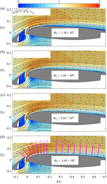
The time-averaged velocity fields and topological streamlines at four typical Rec are shown together in figure 4 to illustrate the integrated topology of the confluent boundary layer above the main element. To reduce the effects of varied flow directions, the resultant velocity contours  $(\sqrt {({U^2} + {V^2})} /{U_\infty })$ are provided, where U and V are the horizontal and vertical components of the mean velocities, respectively. No flow separation is found above the main element. However, with Reynolds numbers (Rec ~ 104) and angles of attack (α ~ 4°) comparable to those of the current work, laminar separation bubbles (LSBs) are prevalent over the NACA0018 airfoil (Istvan & Yarusevych Reference Istvan and Yarusevych2018), NACA0012 airfoil (Jones, Sandberg & Sandham Reference Jones, Sandberg and Sandham2008, Reference Jones, Sandberg and Sandham2010; Wang et al. Reference Wang, Zhou, Alam and Yang2014) and SD7003 airfoil (Burgmann et al. Reference Burgmann, Dannemann and Schröder2008; Burgmann & Schröder Reference Burgmann and Schröder2008; Hain, Kähler & Radespiel Reference Hain, Kähler and Radespiel2009; Olson et al. Reference Olson, Katz, Naguib, Koochesfahani, Rizzetta and Visbal2013). The absence of flow separation can be attributed to the current wake-induced transition (discussed below), which makes the boundary layer above the main element energetic for bearing adverse pressure gradients.
Mean resultant velocity contours with the superimposition of streamlines: (a) Rec = 1.38 × 10⁴; (b) Rec = 1.83 × 10⁴; (c) Rec = 2.41 × 10⁴; and (d) Rec = 3.05 × 10⁴. The velocities are normalized by U∞. The magenta lines in panel (d) define the sampling positions for the velocity and total kinetic energy profiles in figures 5–8. Although the streamlines in PIV1 have been reported by Wang et al. (Reference Wang, Wang and Kim2018b), it is relevant to combine them with the streamlines of PIV2 here for an integrated topology of the confluent boundary above the main element.

The mean resultant velocity and total kinetic energy  $(K/U_\infty ^2)$ are extracted from the sampling positions in figure 4 (magenta lines) for a quantitative description of the confluent boundary layer (figures 5–8). Here K is defined as
 $\tfrac{1}{2}(u_{rms}^2 + v_{rms}^2)$, where
 $u_{rms}$ and
 ${v_{rms}}$ are the root-mean-square values of the streamwise and vertical velocities, respectively. The mean velocity profiles have similar distributions after Rec = 1.83 × 10⁴ (figures 5 and 6). The obvious deviations between the profiles for Rec = 1.38 × 10⁴ and those of the other three Rec values are specifically discussed at the end of this section.
Mean resultant velocity profiles from PIV1. The profiles in (a–h) are extracted from positions 1–8 in figure 4, respectively. Here YL is the local wall-normal coordinate with the origin located at the airfoil surface. The velocities are normalized by U∞. As Rec increases, the profiles are coloured red, blue, magenta and black.

Mean resultant velocity profiles from PIV2. The profiles in (a–h) are extracted from positions 9–16 in figure 4, respectively. Here YL is the local wall-normal coordinate with the origin located at the airfoil surface. The velocities are normalized by U∞. As Rec increases, the profiles are coloured red, blue, magenta and black.

In figure 5, the velocity defect, resulting from slat wakes and marked by VD, recovers downstream (from figure 5a to 5h). This recovery of VD indicates the merging of the slat wake and the original boundary layer of the main element (Thomas, Nelson & Liu Reference Thomas, Nelson and Liu2000). As Rec increases, this merging process is slightly accelerated by the strengthened  $K/U_\infty ^2$ in the slat wake (figure 7a,b). At the initial stage of merging, the outer peak in the slat wake and the inner peak in the original boundary layer of the main element collectively result in a two-peak pattern of
 $K/U_\infty ^2$ in figure 7(a,b). As the merging deepens, the outer peak is weakened by redistributing the
 $K/U_\infty ^2$ of the slat wake into the entire confluent boundary layer (from figure 7b to 7h). The inner peak first increases because of the formation of double-secondary vortices (from figure 7b to 7d) (Wang et al. Reference Wang, Wang and Kim2018b) and then decreases by redistributing the
 $K/U_\infty ^2$ of double-secondary vortices across the entire confluent boundary layer (from figure 7d to 7h). Finally, the two-peak pattern of
 $K/U_\infty ^2$ evolves into a single-peak pattern, further indicating an achieved confluent boundary layer above the main element. The redistribution of
 $K/U_\infty ^2$ across the confluent boundary layer persisted to the rear part of the main element (figure 8) and contributed to the laminar-to-turbulent transition above the main element (discussed in the next section).
Total kinetic energy profiles from PIV1. The profiles in (a–h) are extracted from positions 1–8 in figure 4, respectively. Here YL is the local wall-normal coordinate with the origin located at the airfoil surface. The kinetic energy is normalized by the square of U∞. As Rec increases, the profiles are coloured red, blue, magenta and black.

Total kinetic energy profiles from PIV2. The profiles in (a–h) are extracted from positions 9–16 in figure 4, respectively. Here YL is the local wall-normal coordinate with the origin located at the airfoil surface. The kinetic energy is normalized by the square of U∞. As Rec increases, the profiles are coloured red, blue, magenta and black.

To further characterize the transition of the confluent boundary layer, boundary layer thicknesses and related shape factors at these four typical Rec are provided in figure 9. The boundary thickness δ is defined as the wall-normal distance between the airfoil surface and the boundary layer edge  $(Y_L^{edge})$. The location of
 $Y_L^{edge}$ is at the separatrix between the boundary layer flow and the inviscid free stream (Thomas et al. Reference Thomas, Nelson and Liu2000) and can be determined using the mean spanwise vorticity
 $({\omega _Z} = \partial V/\partial X - \partial U/\partial Y)$ as follows:
(i) Before the merging process is finished, an inviscid free stream is absent between the slat wake and the boundary layer because of the strong wake–boundary layer interactions (figure 5a–d). As an alternative, the separatrix between the positive
 ${\omega _Z}$ of the slat wake and the negative ${\omega _Z}$ of the boundary layer is then defined as $Y_L^{edge}$ to eliminate the effects of the slat wake on the determination of the boundary layer edge. This strategy has also been adopted by He et al. (Reference He, Wang and Pan2013) and Wang et al. (Reference Wang, Feng, Wang and Li2018a).
(ii) After the merging process is finished, the velocity defect related to the slat wake is absent, leading to a fully developed confluent boundary layer above the main element. However, the standard boundary layer assumption (the velocity at the boundary layer edge equals 0.99U∞) remains invalid with the curved surface of the main element. As proposed by Marxen et al. (Reference Marxen, Lang, Rist, Levin and Henningson2009), the wall-normal integration of
${\omega _Z}$ is used to determine $Y_L^{edge}$:
(3.1)\begin{equation}{u_{Integral}} = \int_0^{{Y_L}} {{\omega _Z}\,\textrm{d}{Y_L}} .\end{equation}Finally,
$Y_L^{edge}$ is defined as the position where the variation in ${u_{Integral}}$ vanishes.


Boundary layer parameters above the main element: (a) thickness of the boundary layer and (b) shape factor (H). Here δ is the boundary layer thickness determined by the edge of the boundary layer; δ* is the displacement thickness; θ is the momentum thickness; and Xδ defines the streamwise location of the boundary edge. As Rec increases, the profiles are coloured red, blue, magenta and black. The shape factors of the laminar Blasius boundary layer (H = 2.59) and turbulent boundary layer with zero pressure gradients (H = 1.4) are provided in panel (b) for reference.

Subsequently, the displacement thickness δ*, momentum thickness θ and shape factor H are calculated as follows:
 \begin{gather}{\delta ^\ast } = \int_0^{Y_L^{edge}} {\left( {1 - \frac{{{u_{Integral}}({Y_L})}}{{{u_{Integral}}(Y_L^{edge})}}} \right)\textrm{d}{Y_L},}\end{gather}
 \begin{gather}\theta = \int_0^{Y_L^{edge}} {\left( {1 - \frac{{{u_{Integral}}({Y_L})}}{{{u_{Integral}}(Y_L^{edge})}}} \right)\frac{{{u_{Integral}}({Y_L})}}{{{u_{Integral}}(Y_L^{edge})}}\,\textrm{d}{Y_L}} ,\end{gather}
 \begin{gather}H = \frac{{{\delta ^\ast }}}{\theta }.\end{gather}
The boundary thickness δ is substantially thickened after the slat wake merges with the original boundary layer of the main element (figure 9a). At Rec = 1.38 × 10⁴, the finished position of merging is located at Xδ/c = 0.2. As Rec increases, the merging process is accelerated, leading to the upstream movement of the merging-finished position (within 0.05 < Xδ/c < 0.1 when Rec ≥ 1.83 × 10⁴). After the merging process is finished, δ, δ* and θ collapse well among different Rec, except for Rec = 1.38 × 10⁴. The exception of Rec = 1.38 × 10⁴ will be discussed at the end of this section. As a useful indicator for the laminar-to-turbulent transition, the evolution of H in figure 9(b) clearly illustrates that the confluent boundary layer above the main element develops from a laminar state to a final turbulent state after Rec = 1.83 × 10⁴. The complex wake–shear layer interactions and the accelerated gap flow could be plausible reasons for the larger shape factor (H > 2.59) at the laminar stage. The larger shape factor (H > 1.4) at the rear half of the main element could be attributed to the effects of adverse pressure gradients, similar to the scenarios of turbulent boundary layers over NACA4412 within the Rec interval of 4 × 10⁵ to 1 × 10⁶ (Hosseini et al. Reference Hosseini, Vinuesa, Schlatter, Hanifi and Henningson2016; Vinuesa et al. Reference Vinuesa, Hosseini, Hanifi, Henningson and Schlatter2017, Reference Vinuesa, Negi, Atzori, Hanifi, Henningson and Schlatter2018; Tanarro, Vinuesa & Schlatter Reference Tanarro, Vinuesa and Schlatter2020).
The fluctuation intensities within the boundary layer of the main element are further discussed here for a quantitative description of the above-mentioned transition. Inspired by Wang et al. (Reference Wang, Wang and Kim2018b), the root-mean-square value of  $v^{tran}$
 $(v_{rms}^{tran}/{U_\infty })$ is provided in figure 10 as a reference for the tracking of fluctuation intensities, where
 $v^{tran}$ denotes the fluctuation perpendicular to the main flow direction, and the main flow direction is defined as the direction of the local mean resultant velocity vector. The fluctuation intensities
 $(v_{rms}^{tran}/{U_\infty })$ are then tracked along the black dots of figure 10 and shown in figure 11. The evolution of
 $v_{rms}^{tran}/{U_\infty }$ is found to have similar trends after Rec = 1.83 × 10⁴. Similar to the scenarios of the mean resultant velocity in figures 5 and 6 and of the shape factor in figure 9, obvious deviations between the profile for Rec = 1.38 × 10⁴ and those of the other three Rec values appear in figure 11. Wang et al. (Reference Wang, Wang and Kim2018b) found that Rec = 1.38 × 10⁴ is the lowest Reynolds number for observing slat-wake-triggered double-secondary vortices, and the pattern of double-secondary vortices is accordingly weaker at this Rec. These distinctions of the confluent boundary layer between Rec = 1.38 × 10⁴ and the other three Rec values could therefore be ascribed to the weaker pattern of double-secondary vortices at Rec = 1.38 × 10⁴, indicating the important role of double-secondary vortices in the current wake-induced transition. Although the confluent boundary layer at Rec = 1.38 × 10⁴ evidently deviates from those at the other three Rec values, it is nevertheless further discussed in the next section for comparison.
Root-mean-square contours of  $v^{tran}$ (
 $v_{rms}^{tran}/{U_\infty }$): (a) Rec = 1.38 × 10⁴; (b) Rec = 1.83 × 10⁴; (c) Rec = 2.41 × 10⁴; and (d) Rec = 3.05 × 10⁴. The black dots and magenta crosses are located at the local maxima of
 $v_{rms}^{tran}/{U_\infty }$. The magenta crosses are designed to monitor the local PSDs in the slat wake (cross 1) and in the confluent boundary layer above the main element (crosses 2–9). The black dots are designed to track the fluctuations in the boundary layer above the main element.

Fluctuation tracking along the local maxima of  $v_{rms}^{tran}/{U_\infty }$ (black dots of figure 10). As Rec increases, the related results are coloured red, blue, magenta and black. The dashed orange lines denote the fit of
 $v_{rms}^{tran}/{U_\infty }$ after Rec = 1.83 × 10⁴.

Finally, the current wake-induced transition routine is divided into three stages according to the evolution of  $v_{rms}^{tran}/{U_\infty }$ in the boundary layer after Rec = 1.83 × 10⁴: the initial stage (growth of fluctuations with different growth rates, 0 < X/c < 0.068); the intermediate stage (fast decay of fluctuations, 0.068 < X/c < 0.25); and the late stage (slow decay of fluctuations, X/c > 0.25). Notably, this definition of transition stages is similar to that of He et al. (Reference He, Pan, Feng, Gao and Wang2016) with a simplified circular cylinder–flat plate configuration.
4. Wake-induced transition
In this section, the dynamics of coherent structures across the whole process of the wake-induced transition are discussed in detail. At the initial stage, the wake disturbances penetrate the boundary layer of the main element and are then amplified exponentially, leading to slat-wake-triggered double-secondary vortices. At the intermediate stage, the wake disturbances continue to trigger the three-dimensional destabilization of the secondary vortices by direct injection or indirect induction, generating Λ vortices. At the late stage, Λ vortices evolve into hairpin vortex packets and finally contribute to an attached turbulent boundary layer above the main element.
4.1. Initial stage
The slat-wake-triggered double-secondary vortices at a typical Reynolds number, Rec = 1.83 × 10⁴, are revisited by VDV in figure 12. Compared to the hydrogen bubble visualization with a single streaky line (Wang et al. Reference Wang, Wang and Kim2018b), virtual dyes with different colours can simultaneously visualize the interactions of flow patterns between the slat wake and the boundary layer of the main element. It is more instructive to reveal that two secondary vortices ( $V_M^1$ and
 $V_M^2$ in figure 12) are triggered by one shed vortex of the slat cusp shear layer (VS in figure 12). Furthermore, figure 12(e) indicates that the double-secondary vortices introduce prominent velocity fluctuations into the boundary layer of the main element and play an important role in the current wake-induced transition.
Revisiting of slat-wake-triggered double-secondary vortices at Rec = 1.83 × 10⁴ by VDV: (a) t; (b) t + Δt; (c) t + 2Δt; and (d) t + 3Δt. (e) A zoomed-in view of (d) with the superimposition of fluctuating velocity vectors. Here Δt/T = 0.37, where T is the shedding period of VS; VS denotes the shed vortex of the slat cusp shear layer; and  $V_M^1$ and
 $V_M^2$ denote the two vortices in one topology of double-secondary vortices. The virtual dyes in blue and red are designed to mimic the hydrogen bubble visualization for flow structures of the slat wake and above the main element in Wang et al. (Reference Wang, Wang and Kim2018b), respectively. The green virtual dye is designed to visualize the flow structures originating from the upper boundary layer of the slat.

The strategy of fluctuation tracking within different frequency bands (Simoni et al. Reference Simoni, Ubaldi, Zunino, Lengani and Bertini2012; Wang et al. Reference Wang, Feng, Wang and Li2018a) is shown in figures 13 and 14 to describe the effects of double-secondary vortices on the initial stage of the wake-induced transition. The  $v^{tran}$ signals are extracted from the probes (marked by magenta crosses) of figure 10 to calculate the local PSDs in figure 13, which provides related frequency bands for fluctuation tracking. Different types of frequency peaks appear in figure 13. The recent study of Wang & Wang (Reference Wang and Wang2021) discussed the flow physics behind these frequency peaks in the slat wake: (i) the shed vortices of the slat cusp shear layer (VS) generate disturbances of the fundamental frequency (St1) and harmonics (St2 and St3) during their formation and subsequent deformations (local power spectral densities at probe 1 of figure 13); (ii) as Rec increases (2.41 × 10⁴ ≤ Rec ≤ 3.05 × 10⁴), VS impinges on the underside of the slat trailing edge with unsteady locations, leading to disturbances of subharmonics (St0.5 at probe 1 of figure 13c, St0.36 and St0.66 at probe 1 of figure 13d); and (iii) the secondary instability in the braid region of VS contributes to disturbances of the fractional harmonics (St1.36 and St1.66 at probe 1 of figure 13d).
Local PSDs of  $v^{tran}$ during the formation of double-secondary vortices: (a) Rec = 1.38 × 10⁴; (b) Rec = 1.83 × 10⁴; (c) Rec = 2.41 × 10⁴; and (d) Rec = 3.05 × 10⁴. The PSDs are calculated at crosses 1–6 in figure 10 and remain marked by the same magenta numbers as in figure 10. For clarity, the amplitude of each PSD is amplified step by step by 104 along the streamwise direction. Labels St1, St2 and St3 denote the fundamental frequency, second harmonic and third harmonic, respectively; St0.5 in (c) and St0.36 and St0.66 in (d) denote the subharmonics; and St1.5 and St2.5 in (c) and St1.36 and St1.66 in (d) denote the fractional harmonics. The subscripts of St denote the ratios of peak frequencies to the fundamental frequency. The VF1 and VFS bands contain the fluctuations pertaining to the fundamental frequency and all the frequency peaks, respectively.

Spatial growth of the fluctuations within different frequency bands: (a) Rec = 1.38 × 10⁴; (b) Rec = 1.83 × 10⁴; (c) Rec = 2.41 × 10⁴; and (d) Rec = 3.05 × 10⁴. The fluctuations are extracted from the black dots of figure 10. The red dashed lines denote the exponential fittings. Here S/c represents the curvilinear coordinate located at the local peaks of  $v_{rms}^{tran}/{U_\infty }$, and the origin of S/c is defined at the first point of the black dots in figure 10; and X/c shows the streamwise locations of a specific S/c with the coordinates defined in figure 1.

Consistent with the scenarios of the fundamental frequency and harmonics (Wang et al. Reference Wang, Wang and Kim2018b), the FMD modes of the current work (not shown for conciseness) reveal that the subharmonics and fractional harmonics in the slat wake can also penetrate the boundary layer of the main element (probes 2–6 in figure 13c,d) and be related to the vortex dynamics of  $V_M^1$ and
 $V_M^2$. Therefore, VF1 and VFS are designed in figure 13 to contain the fluctuations pertaining to the fundamental frequency and all the frequency peaks, respectively. The quantitative intervals of the VF1 and VFS bands are provided in table 1. The resulting fluctuation intensities within these two bands are, respectively, denoted
 $v_{rms}^{V{F^1}}/{U_\infty }$ and
 $v_{rms}^{V{F^S}}/{U_\infty }$ in figure 14. The
 $v_{rms}^{tran}/{U_\infty }$ at the initial stage of figure 11 are also shown in figure 14 (as
 $v_{rms}^{All}/{U_\infty }$) for convenient comparisons. In addition, after removing the fluctuations within the VF1 band from those within the VFS band, the contributions of different types of harmonics to
 $v_{rms}^{All}/{U_\infty }$ are emphasized in figure 14
 $(v_{rms}^{V{F^S} - V{F^1}}/{U_\infty })$. It is found that
 $v_{rms}^{All}/{U_\infty }$ increases exponentially during the formation of
 $V_M^1$ (X/c < 0.04 in figure 14a and X/c < 0.024 in figure 14b–d), although it is affected by strong wake disturbances. Moreover,
 $v_{rms}^{V{F^1}}/{U_\infty }$ and
 $v_{rms}^{V{F^S} - V{F^1}}/{U_\infty }$ also increase exponentially. When the double-secondary vortices become prominent (Rec ≥ 1.83 × 10⁴) (Wang et al. Reference Wang, Wang and Kim2018b),
 $v_{rms}^{V{F^1}}/{U_\infty }$ decreases and
 $v_{rms}^{V{F^S} - V{F^1}}/{U_\infty }$ continues to increase during the formation of
 $V_M^2$ (approximately 0.024 < X/c < 0.068 in figure 14b–d). The increase in
 $v_{rms}^{V{F^S} - V{F^1}}/{U_\infty }$ leads to the exponential secondary growth of
 $v_{rms}^{All}/{U_\infty }$ (figure 14b–d). Consequently, the fluctuations at the initial stage of the transitional confluent boundary layer possess double-exponential growth (figure 14b–d). The similarity between
 $v_{rms}^{All}/{U_\infty }$ and
 $v_{rms}^{V{F^S}}/{U_\infty }$ in figure 14(b–d) further verifies that the double-exponential growth of
 $v_{rms}^{All}/{U_\infty }$ is due to the formation of double-secondary vortices. In contrast, the weak pattern of double-secondary vortices at Rec = 1.38 × 10⁴ leads to a continued increase in
 $v_{rms}^{V{F^1}}/{U_\infty }$ and a flat distribution of
 $v_{rms}^{V{F^S} - V{F^1}}/{U_\infty }$ after the formation of
 $V_M^1$ (X/c > 0.04 in figure 14a). Consequently, the double-exponential growth of
 $v_{rms}^{All}/{U_\infty }$ after Rec = 1.83 × 10⁴ is absent at Rec = 1.38 × 10⁴ (figure 14a). However, the evolution of
 $v_{rms}^{V{F^S}}/{U_\infty }$ at Rec = 1.38 × 10⁴ remains similar to that of
 $v_{rms}^{All}/{U_\infty }$ (figure 14a), consistent with the scenarios at the other three Rec values (figure 14b–d). Notably, the spanwise (VS) and streamwise vortices are present in the slat wake (Wang et al. Reference Wang, Wang and Kim2018b). Because
 $v_{rms}^{V{F^S}}/{U_\infty }$ originates from the wake disturbances related to the spanwise vortices, the similarity between
 $v_{rms}^{All}/{U_\infty }$ and
 $v_{rms}^{V{F^S}}/{U_\infty }$ in figure 14 could indicate that the confluent boundary layer first responds to the disturbances of spanwise vortices rather than those of streamwise vortices at the initial stage of transition.
The quantitative intervals of VF1 and VFS bands at different Rec.

The exponential growth of fluctuations during the formation of secondary vortices is similar to the ‘wake-triggered single-secondary vortex’ case in He et al. (Reference He, Wang and Pan2013). However, the current wake-induced transition at the initial stage is intrinsically different from that of He et al. (Reference He, Wang and Pan2013). First, limited by the simplified geometry, the wake disturbances in He et al. (Reference He, Wang and Pan2013) only mildly affect the boundary layer, leading to relatively weak secondary vortices. In contrast, the disturbances of the slat wake affect the boundary layer in a stronger way. As a result, the  $v_{rms}^{All}/{U_\infty }$ originating from the single-secondary vortex is one order of magnitude lower than that of the current double-secondary vortices (He et al. Reference He, Wang and Pan2013; He & Wang Reference He and Wang2015). Second, the double-secondary vortices cause the fluctuations to exhibit double-exponential growth (figure 14), which is absent during the formation of a single-secondary vortex in He et al. (Reference He, Wang and Pan2013).
4.2. Intermediate stage
At the intermediate stage, the secondary vortices evolve into Λ vortices due to three-dimensional instability, similar to the scenarios of simplified circular cylinder–flat plate configurations (Pan et al. Reference Pan, Wang, Zhang and Feng2008; Mandal & Dey Reference Mandal and Dey2011; He et al. Reference He, Wang and Pan2013; He et al. Reference He, Pan, Feng, Gao and Wang2016). This process at the typical Reynolds number of Rec = 1.83 × 10⁴ is visualized in figure 15. A spanwise  $V_M^1$ in one pattern of double-secondary vortices is convected downstream and finally evolves into several Λ vortices distributed along the spanwise direction. These Λ vortices maintain their coherences and are further convected to the rear part of the main element. For clarity, one of these Λ vortices is magnified in figure 15(g) with a sketched skeleton. The evolution of secondary vortices at Rec = 1.38 × 10⁴ is also provided in figure 16 for comparison. The generation process of Λ vortices due to the three-dimensional destabilization of spanwise secondary vortices still occurs in the boundary layer of the main element at Rec = 1.38 × 10⁴ (figure 16), although the confluent boundary layer at this Rec value evidently deviates from those at the other three Rec values (discussed in § 3).
Hydrogen bubble visualization of the flow structures above the main element at Rec = 1.83 × 10⁴. Panels (a–i) show a time sequence with an interval of Δt/T = 0.35 between two consecutive instants. Label  $V_M^1$ denotes one vortex of double-secondary vortices. The bottom left corner of (g) zooms in the pattern of a Λ vortex. Here
 ${Z_1}$ denotes the local spanwise coordinate with the origin located to the left of the field of view.

Hydrogen bubble visualization of the flow structures above the main element at Rec = 1.38 × 10⁴. Panels (a–i) show a time sequence with an interval of Δt/T = 0.30 between two consecutive instants. Label  $V_M^1$ denotes one vortex of double-secondary vortices. The bottom left corner of (g) zooms in the pattern of a Λ vortex. Here
 ${Z_1}$ denotes the local spanwise coordinate with the origin located to the left of the field of view.

The Λ vortices evolving from the secondary vortices are also captured in PIV3 (figure 17). The pattern marked by the black box in figure 17(a) shows the cross-section of two legs in one Λ vortex. The velocity vectors of the zoom-in view (figure 17b) clearly visualize the upstream induction between the two legs of this Λ vortex. To further build the connections between secondary vortices and the resulting Λ vortices, FMD is applied to the streamwise velocity fluctuations of PIV3 (figures 18 and 19). The fundamental frequency of the global PSD (St1 of figure 18) couples with that of figure 13 at each Rec. This coupling indicates that the FMD mode of St1 extracts the flow patterns related to the secondary vortices (figure 19). The spanwise patterns in figure 19 (marked by magenta boxes) reveal the two-dimensional properties of secondary vortices during their formation, consistent with Wang et al. (Reference Wang, Wang and Kim2018b). As the legs of Λ vortices are convected downstream, staggered patterns appear in the FMD modes, one of which at Rec = 1.83 × 10⁴ is marked by a magenta circle in figure 19(b). The simultaneous occurrence of spanwise secondary vortices and Λ vortices in one FMD mode verifies the strong correlation between them. In addition, this correlation further demonstrates that the consequent Λ vortices inherit the periodicities of double-secondary vortices at the intermediate stage of transition. Notably, the Λ vortices promote mixing within the confluent boundary layer by the inductions visualized in figure 17(b). This mixing could be responsible for the energy redistribution mentioned in § 3 and the decrease in  $v_{rms}^{All}/{U_\infty }$ around X/c > 0.068 (figure 11).
Instantaneous vorticity contours ( ${\omega _Y}c/{U_\infty }$) of the plan view PIV3 at Rec = 1.83 × 10⁴: (a) overview; and (b) enlarged Λ vortex with the superimposition of velocity vectors in the black box of panel (a). The black line in (a) marks the leading edge of the main element. The flow structures in the slat wake are marked by the magenta box in (a). Here
 ${Z_2}$ denotes the local spanwise coordinate with the origin located to the left of the field of view.

Global PSDs of streamwise velocity fluctuations from PIV3: (a) Rec = 1.38 × 10⁴; (b) Rec = 1.83 × 10⁴; (c) Rec = 2.41 × 10⁴; and (d) Rec = 3.05 × 10⁴. Label St1 marks the fundamental frequency.

FMD modes of the fundamental frequencies in figure 18: (a) Rec = 1.38 × 10⁴; (b) Rec = 1.83 × 10⁴; (c) Rec = 2.41 × 10⁴; and (d) Rec = 3.05 × 10⁴. Only the mode of streamwise velocity fluctuations is provided here. The pattern of Λ vortices is marked by the magenta ellipse in (b). The black lines mark the leading edge of the main element. Here  ${Z_2}$ denotes the local spanwise coordinate with the origin located to the left of the field of view.

As visualized in figure 12, the slat wake rides above the double-secondary vortices. Streamwise vortices are present in the slat wake (Wang et al. Reference Wang, Wang and Kim2018b) and are captured in figure 17 with a cross-sectional view (marked by a magenta box). Whether the three-dimensional instability of secondary vortices is affected by the disturbances in the slat wake, especially in relation to the streamwise vortices, will be further discussed here. The TPC introduced in § 2.2.3 is used to evaluate the spanwise wavelengths of disturbances in the slat wake (reference position  ${X_{ref}}/c = 0$) and of Λ vortices
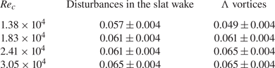
 $({X_{ref}}/c = 0.2)$. The spanwise ‘replication’ of flow structures leads to alternate distributions of positive and negative R in the spanwise direction (figure 20). The R profiles are further extracted from the reference positions in figure 20 and shown in figure 21 for the determination of spanwise wavelengths. As revealed in Wang, Pan & Wang (Reference Wang, Pan and Wang2019), the spanwise wavelengths of related flow patterns are defined as the distances between the minima of R profiles (marked by red crosses in figure 21). The spanwise wavelength of the Λ vortices couples with that of the disturbances in the slat wake at each Rec (table 2). These couplings strongly indicate that the destabilization of spanwise secondary vortices to the Λ vortices is triggered by the disturbances in the slat wake, consistent with the conjecture in He et al. (Reference He, Pan, Feng, Gao and Wang2016). As a result, a new question arises: How does the slat wake trigger the three-dimensional instability of spanwise secondary vortices?
The TPC contours of PIV3: (a) Rec = 1.38 × 10⁴; (b) Rec = 1.83 × 10⁴; (c) Rec = 2.41 × 10⁴; and (d) Rec = 3.05 × 10⁴. The magenta dashed lines represent the reference positions for the TPC. The lines located at X/c = 0 and X/c = 0.2 are designed to extract the spanwise wavelengths of the slat wake (S-W) and Λ vortices (Λ-V), respectively. Here  ${Z_2}$ denotes the local spanwise coordinate with the origin located to the left of the field of view.

The TPC profiles extracted from the reference positions of figure 20: (a) Rec = 1.38 × 10⁴; (b) Rec = 1.83 × 10⁴; (c) Rec = 2.41 × 10⁴; and (d) Rec = 3.05 × 10⁴. The profiles in the slat wake (S-W) and the profiles related to the Λ vortices (Λ-V) are denoted by black lines with dots and blue lines with upward-pointing triangles, respectively. The minima of R are marked by red crosses. Here  ${Z_2}$ denotes the local spanwise coordinate with the origin located to the left of the field of view.

Normalized spanwise wavelengths (by c) at different Rec values.

The VDV is again applied to Rec = 1.83 × 10⁴ to answer this question (figure 22). For the sequence of figure 22(a,c,e,g), the deformed VS is convected downstream and does not touch the  $V_M^1$ and
 $V_M^2$ triggered by it. Therefore, the disturbances in the slat wake could trigger the three-dimensional instability of secondary vortices by indirect induction. For the sequence of figure 22(b,d,f,h), after triggering
 $V_M^1$ and
 $V_M^2$, the deformed VS is further entrained into
 $V_M^1$. Consequently, the disturbances in the slat wake could be directly injected into
 $V_M^1$, leading to the three-dimensional instability of secondary vortices. As the products of three-dimensional instability, the Λ vortices inherit the spanwise wavelength of the disturbances in the slat wake by indirect induction and direct injection mechanisms. These two mechanisms are also universal for the other three Rec values (figure 23). The typical scenarios of indirect induction and direct injection at the other three Rec values are provided in the left and right columns of figure 23, respectively. As discussed in § 3, the weak pattern of slat-wake-triggered double-secondary vortices in figure 23(a,b) could be ascribed to the lowest Reynolds number of Rec = 1.38 × 10⁴ (Wang et al. Reference Wang, Wang and Kim2018b).
Wake-triggered three-dimensional instability of secondary vortices at Rec = 1.83 × 10⁴. Panels (a,c,e,g) and (b,d,f,h) are two time sequences with Δt/T = 0.37. Panels (a,c,e,g) show the indirect induction of the slat wake for triggering the three-dimensional instability. Panels (b,d,f,h) show the direct injection of the slat wake to trigger the three-dimensional instability. Here VS denotes the shed vortex of the slat cusp shear layer; and  $V_M^1$ and
 $V_M^2$ denote the two vortices in one topology of double-secondary vortices.

Wake-triggered three-dimensional instability of secondary vortices: (a,b) Rec = 1.38 × 10⁴; (c,d) Rec = 2.41 × 10⁴; and (e,f) Rec = 3.05 × 10⁴. Panels (a,c,e) show the indirect induction of the slat wake for triggering the three-dimensional instability. Panels (b,d,f) show the direct injection of the slat wake for triggering the three-dimensional instability. Here VS denotes the shed vortex of the slat cusp shear layer; and  $V_M^1$ and
 $V_M^2$ denote the two vortices in one topology of double-secondary vortices.

4.3. Late stage
At the late stage of transition (Rec ≥ 1.83 × 10⁴), an attached turbulent boundary layer, affected by adverse pressure gradients, is achieved above the main element (figure 9). The dynamics of coherent structures at this stage will be further explored in this section.
As mentioned in § 4.2, the Λ vortices inherit the periodicities of secondary vortices at the intermediate stage of transition. However, this type of periodicity is unnecessary for a turbulent boundary layer. Fortunately, these Λ vortices lose periodicity as they are convected to the rear part of the main element. The frequency peaks (St1 and St2) at each Rec are therefore weakened and finally vanish along the streamwise direction (figure 24). As Rec increases, the vanishing periodicity is accelerated.
Local PSDs of  $v^{tran}$ at the late stage of the transitional confluent boundary layer: (a) Rec = 1.38 × 10⁴; (b) Rec = 1.83 × 10⁴; (c) Rec = 2.41 × 10⁴; and (d) Rec = 3.05 × 10⁴. The PSDs are calculated at crosses 7–9 of figure 10 and remain marked by the same magenta numbers as in figure 10. For clarity, the amplitude of each PSD is amplified step by step by 104 along the streamwise direction. Labels St1 and St2 denote the fundamental frequency and second harmonic, respectively.

To further characterize the coherent structures at the late stage of transition, FTLEs are used to track the LCSs around the centre part of the main element (figures 25 and 26). Adrian (Reference Adrian2007), Pan et al. (Reference Pan, Wang, Zhang and Feng2008) and He et al. (Reference He, Pan, Feng, Gao and Wang2016) have shown that the Λ vortices generated at the intermediate transition stage could evolve into hairpin vortices. Zhou et al. (Reference Zhou, Adrian, Balachandar and Kendall1999) noted that the self-reproduction of hairpin vortices could lead to hairpin vortex packets. As indicated by He et al. (Reference He, Pan, Feng, Gao and Wang2016), figure 25 demonstrates that the hairpin vortex packets are universal in the boundary layer above the main element, similar to the scenarios of simplified circular cylinder–flat plate configurations (Pan et al. Reference Pan, Wang, Zhang and Feng2008; He et al. Reference He, Pan, Feng, Gao and Wang2016).
Hairpin vortex packets revealed by FTLEs: (a) Rec = 1.38 × 10⁴; (b) Rec = 1.83 × 10⁴; (c) Rec = 2.41 × 10⁴; and (d) Rec = 3.05 × 10⁴.

The generation process of a typical hairpin vortex packet at Rec = 1.83 × 10⁴. Panels (a–d) show a time sequence with Δt/T = 0.55. Arrows A, D and E mark three original hairpin vortices. Arrows B and C mark two hairpin vortices reproduced by A. Arrows F and G mark two hairpin vortices reproduced by E.

For the sake of brevity, only the formation of one typical hairpin vortex packet at Rec = 1.83 × 10⁴ is described in figure 26. The primary hairpin vortex A reproduces the second hairpin vortex B and the third hairpin vortex C. Moreover, the primary hairpin vortex E reproduces the second hairpin vortex F and the third hairpin vortex G. Ultimately, the primary hairpin vortices (A, E and D) and the reproduced hairpin vortices (B, C, F and G) establish a hairpin vortex packet above the main element (figure 26d). Similar to Pan et al. (Reference Pan, Wang, Zhang and Feng2008) and He et al. (Reference He, Pan, Feng, Gao and Wang2016), the upward inductions of hairpin vortex legs induce streaky structures within the boundary layer, which are revealed by the POD modes in figure 27. As the significant skeletons of turbulent boundary layers (Adrian Reference Adrian2007), hairpin vortex packets and streaky structures could entangle with each other to promote the establishment of a self-sustaining turbulent boundary layer above the main element. Notably, the momentum-thickness Reynolds number (Reθ) of the boundary layer above the main element (e.g. Reθ = 300 around X/c = 0.6 at Rec = 1.83 × 10⁴) is low for a common turbulent boundary layer over a flat plate. However, the current turbulent flow above the main element is generated by the wake-induced transition. The strong wake disturbances could continuously provide energy by triggering double-secondary vortices and their subsequent three-dimensional destabilization to sustain the turbulent flow at such a low Reθ.
POD modes of streamwise velocity fluctuations around the centre part of the main element (PIV4): (a) Rec = 1.38 × 10⁴; (b) Rec = 1.83 × 10⁴; (c) Rec = 2.41 × 10⁴; and (d) Rec = 3.05 × 10⁴. Only the first mode is provided at each Rec. Here  ${Z_3}$ denotes the local spanwise coordinate with the origin located to the left of the field of view.

5. Concluding remarks
In the current work, the wake-induced transition over a 30P30N multi-element airfoil (α = 4°) is explored at low Reynolds numbers (1.38 × 10⁴ ≤ Rec ≤ 3.05 × 10⁴) using time-resolved particle image velocimetry and hydrogen bubble visualization. The uniqueness of this study lies in the detailed discussions of the special laminar-to-turbulent transition routine in the confluent boundary layer over the main element. To the best of the authors’ knowledge, such comprehensive analyses with similar geometries have not been presented before. The effects of slat-wake-triggered double-secondary vortices on the entire transition process are particularly highlighted. Furthermore, two mechanisms are proposed to characterize how the disturbances in the slat wake affect the three-dimensional destabilization of secondary vortices. It is hoped that the flow physics behind the current transition routine can promote a deeper understanding of low-Reynolds-number flows over multi-element airfoils.
The integrated transition routine is sketched in figure 28 according to the dynamics of coherent structures. At the initial stage, the boundary layer of the main element first responds to the wake disturbances related to the spanwise shed vortices of the slat cusp shear layer, rather than those related to the streamwise vortices (legs of hairpin-like vortices). These wake disturbances penetrate the boundary layer of the main element and are then amplified by double-exponential growth to generate double-secondary vortices. At the intermediate stage, the boundary layer of the main element begins to respond to the disturbances related to the streamwise vortices in the slat wake. These wake disturbances trigger the three-dimensional destabilization of secondary vortices by direct injection or indirect induction, leading to Λ vortices. The spanwise wavelength of the consequent Λ vortices is therefore locked on by the disturbances in the slat wake. These Λ vortices could enhance the mixing and therefore redistribute the fluctuation energies of secondary vortices across the boundary layer, accelerating the formation of a turbulent boundary layer. At the late stage, Λ vortices could evolve into hairpin vortices and hairpin vortex packets. The induction of hairpin vortex legs further results in streaky structures in the boundary layer. As the significant skeletons of turbulent boundary layers, these two patterns could promote the establishment of a turbulent boundary layer above the main element. Throughout the transition process, no obvious separation occurs in the mean flow above the main element, indicating potential aerodynamic benefits.
Sketch of the wake-induced transition over the main element. The hairpin-like vortices in the slat wake are highlighted in Wang et al. (Reference Wang, Wang and Kim2018b). Aiming at a clear depiction of the flow physics above the main element, only three cycles of wake vortices are provided in the upper sketch. Notably, these wake vortices are convected downstream after being formed. The slat in the lower sketch is moved upstream for a clear depiction of the flow physics above the main element.

Compared to the simplified circular cylinder–flat plate configurations, the 30P30N multi-element airfoil is more relevant to engineering practice. The increased complexities of geometry and pressure distribution lead to evident distinctions of the wake-induced transition between simplified configurations (Pan et al. Reference Pan, Wang, Zhang and Feng2008; He et al. Reference He, Wang and Pan2013; He et al. Reference He, Pan, Feng, Gao and Wang2016) and that of the current work. The increased geometrical complexity makes the wake disturbances affect the boundary layer in a stronger way. During the formation of secondary vortices, the fluctuation intensity in the current transitional boundary layer is therefore one order of magnitude higher than that with a simplified configuration (He et al. Reference He, Wang and Pan2013; He & Wang Reference He and Wang2015). In addition, the double-secondary vortices cause the fluctuations to possess double-exponential growth, which is absent during the formation of a single-secondary vortex in He, Wang & Pan (Reference He, Wang and Pan2013). Because of the adverse pressure gradients above the main element, the final turbulent boundary layer has a larger shape factor than that in Pan et al. (Reference Pan, Wang, Zhang and Feng2008) with zero pressure gradients.
Reliable three-dimensional databases of the flows over multi-element airfoils could further deepen the comprehension of the three-dimensional destabilization of secondary vortices. These reliable three-dimensional databases should be pursued in future work.
Acknowledgements
The authors thank Dr Guosheng He, Dr Xi Chen and Yanguang Long for many fruitful discussions regarding this work.
Funding
The authors acknowledge the financial support of the National Natural Science Foundation of China (91852206, 11721202).
Declaration of interests
The authors report no conflict of interest.