





1 Introduction
Instabilities in fluid dynamics are caused by some feedback mechanism and are typically described by governing equations in the form of coupled differential equations. Here we study the case of thermoacoustic instabilities, where the feedback is between the acoustic field and the heat release rate in a combustor. A special feature of this type of instability is the delayed feedback. This leads to a class of governing equations that are characterised by a delay term. Delay differential equations are not well studied in fluid dynamics. We sidestep them by turning our governing equations into a delay integral equation by using an approach based on the tailored Green’s function. We will then illustrate that this can be solved with simple techniques, giving stability predictions quickly and without much numerical effort. Our approach is very general and likely to be of benefit to other branches of fluid dynamics.
When a heat source, such as a flame or hot-wire gauze, is situated in a cavity, thermoacoustic feedback can occur between the heat source and the acoustic field in the cavity, and this may result in intense oscillations. This effect is termed ‘thermoacoustic instability’. The pressure amplitudes may be as high as 2 % of the mean pressure in the cavity (see Scarinci Reference Scarinci, Lieuwen and Yang2005). Combustion systems that are prone to suffering thermoacoustic instabilities include domestic heating systems, gas turbines, rockets, furnaces and afterburners of jet aircraft. The oscillations may be so violent that they cause structural damage; for example, Goy, James & Rea (Reference Goy, James, Rea, Lieuwen and Yang2005) report the destruction of a combustion liner and a burner assembly.
Thermoacoustic instabilities were discovered in the nineteenth century by Higgins (Reference Higgins1802) and Rijke (Reference Rijke1859). They received much attention by rocket engineers in the 1950s and 1960s during the development of liquid-propellant rocket engines (Crocco & Cheng Reference Crocco and Cheng1956). More recently, they have again become the focus of intense research due to increased environmental awareness, demanding the development of combustion systems with reduced emission of pollutants, in particular CO
 $_{2}$
and NO
 $_{x}$
. Modern combustion concepts satisfy the low-emission requirement by operating with premixed flames in the lean regime. However, this concept brings a new problem: its implementation makes a combustion system more susceptible to thermoacoustic instabilities, and these can occur suddenly and spontaneously.
A vast amount of literature on thermoacoustic instabilities has been produced over the years. One can get an overview in the review articles of Candel (Reference Candel2002), Lieuwen (Reference Lieuwen2003) and Huang & Yang (Reference Huang and Yang2009), in the books by Lieuwen & Yang (Reference Lieuwen and Yang2005) and Poinsot & Veynante (Reference Poinsot and Veynante2005), and in Culick (Reference Culick2006). The basic mechanism responsible for thermoacoustic instability is well understood: a flame with a varying rate of heat release acts like a sound source, generating sound waves. The sound waves in turn affect the heat release rate, since they are reflected at the cavity boundaries, and then travel back to the flame. The phase of these reflected waves may be such that the heat release rate is increased, and, in such a case, a mutual enhancement of the sound field and heat-release-rate oscillations ensues. The frequency of such an unstable oscillation is typically close to one of the resonance frequencies of the cavity.
Thermoacoustic nonlinearities are typically due to the interaction between heat release rate and the acoustic field, whereas nonlinearities in the acoustic field itself are unimportant in most cases (Culick Reference Culick2006). They manifest themselves in effects such as limit cycle oscillations, triggering, hysteresis, quasi-periodic oscillations and chaos. Various approaches have been used to study nonlinear effects in combustion systems, including experimental, numerical and analytical methods, or a combination of them.
Test rigs of various designs have been used for experimental nonlinear studies. The horizontal Rijke tube is the most basic system to exhibit thermoacoustic nonlinearities. It is a tube with two open ends, a mean flow through the tube, and a compact heat source (typically an electrically heated wire grid) inside the tube. The main parameters that can be varied are the position and power of the heat source, as well as the mean flow speed. Heckl (Reference Heckl1990) performed experiments where she measured the heater transfer matrix for different velocity amplitudes and then deduced a semi-empirical nonlinear correlation between the heat release rate and the velocity. Matveev & Culick (Reference Matveev and Culick2003a ,Reference Matveev and Culick b ) worked with a similar set-up; they measured limit cycle amplitudes for different heater powers, and they observed the presence of hysteresis. Similar results were reported by Mariappan (Reference Mariappan2012), who also used heater power as control parameter. Also using a horizontal Rijke tube, Gopalakrishnan & Sujith (Reference Gopalakrishnan and Sujith2014) have made detailed measurements to investigate how three of the system parameters (heater power, heater location and mass flow rate) influence the hysteresis characteristics. In a subsequent experimental and numerical study (Gopalakrishnan & Sujith Reference Gopalakrishnan and Sujith2015), they found that external noise reduces the width of the hysteresis zone.
Experimental nonlinear studies have also been performed on flame-driven laboratory test rigs. Noiray et al. (Reference Noiray, Durox, Schuller and Candel2008) developed a burner where the cavity was a tube with one closed end and one open end (quarter-wave resonator), and the heat source was a two-dimensional (2D) array of many small flames (matrix flame), situated close to the open end. The tube length could be adjusted continuously and was used as control parameter. The amplitude-dependent transfer function relating the heat release rate and acoustic velocity in the frequency domain (flame describing function, or FDF) was measured. The experiment revealed linear and nonlinear stability boundaries, limit cycles and hysteresis. Mode switching and instability triggering was also observed. Kabiraj & Sujith (Reference Kabiraj and Sujith2012) studied a set-up consisting of a quarter-wave resonator with a laminar conical premixed flame. As they moved the flame position along the tube axis, they observed a sequence of transitions: (i) from stable flame to limit cycle oscillations via a subcritical Hopf bifurcation, (ii) to quasi-periodic oscillations, (iii) to intermittent oscillations, and finally (iv) to flame blow-out. Nair & Sujith (Reference Nair and Sujith2014) experimented on a laboratory-scale turbulent dump combustor with a premixed flame. They progressively increased the air flow rate and studied the transition from low-amplitude aperiodic oscillations (combustion noise) to high-amplitude periodic oscillations (thermoacoustic instability). They discovered that the multifractal nature of the combustion noise disappears during this transition and conclude that this feature has prognostic value in that it can predict an impending thermoacoustic instability.
There are many numerical studies (linear and nonlinear) on thermoacoustic instabilities. Combustion computational fluid dynamics (CFD) is the method of choice for modelling test rigs with complicated geometry and flow structures. However, this is computationally expensive because combustion is a multiscale problem, with length scales ranging from less than 1 mm (flame front thickness) to more than 1 m (acoustic wavelength). Several methodologies, with varying degrees of resolution and corresponding computational effort, are available. The unsteady Reynolds-averaged Navier–Stokes (URANS) method requires relatively low computational effort; it has been used by many researchers, for example Armitage et al. (Reference Armitage, Balachandran, Mastorakos and Cant2006) or Shahi et al. (Reference Shahi, Kok, Roman Casado and Pozarlik2015), and is popular in the industrial research community. Large eddy simulation (LES), used for example by Franzelli et al. (Reference Franzelli, Riber, Gicquel and Poinsot2012) or Tay-Wo-Chong & Poplifke (Reference Tay-Wo-Chong and Poplifke2013), is more accurate, but requires high-performance computing. Direct numerical simulation (DNS) produces predictions from first principles, capturing even the smallest scales; however, it requires an extreme amount of numerical effort and is only used for fundamental research, e.g. by Talei, Hawkes & Brear (Reference Talei, Hawkes and Brear2013) and Wang et al. (Reference Wang, Luo, Yi and Fan2013). In addition to multiple length scales, combustion modelling may involve multiple time scales, and this requires further numerical effort. This applies, for example, to acoustic disturbances that have a large frequency to growth-rate ratio, i.e. that grow or decay slowly in time. Combustion CFD then requires the calculation of a large number of cycles with high temporal accuracy. Moreover, combustion CFD only gives limited physical insight because it is impossible to separate individual physical processes.
Analytical methods come into their own when physical insight is a priority. The most commonly used methods for nonlinear problems in thermoacoustics are network modelling, the Galerkin method and adjoint optimisation.
Network modelling is a well-known linear concept, and is done in the frequency domain. It involves calculating the complex eigenfrequencies, and deducing the stability behaviour from the sign of their imaginary part. It can still be applied in a quasi-linear fashion for cases where the heat source is described by an amplitude-dependent flame transfer function. This amplitude-dependent network modelling gives a surprisingly large range of predictions, as has been shown by Noiray et al. (Reference Noiray, Durox, Schuller and Candel2008): linear/nonlinear stability, limit cycle amplitudes, mode switching and instability triggering. However, the method is limited to cases where one mode dominates; it is unsuitable for cases where harmonics of the dominant mode come into play.
A more general method for analysing thermoacoustic oscillations is the Galerkin expansion, which goes back to Zinn & Lores (Reference Zinn and Lores1971). The acoustic field in the combustion chamber is written as a sum of basis functions, termed ‘Galerkin modes’, with time-varying coefficients. The Galerkin modes are chosen to be the acoustic eigenmodes of the combustion chamber, which satisfy the relevant boundary conditions. The time-varying coefficients are calculated from a coupled set of nonlinear ordinary differential equations (ODEs). These are solved numerically, and one then obtains the time history of the thermoacoustic oscillation. The Galerkin method works well for systems, where the eigenfunctions are given by simple analytical expressions, e.g. by
 $\sin (n{\rm\pi}x/L)$
for mode
 $n$
of the acoustic pressure in a tube of length
 $L$
with open ends. This is the case for the horizontal Rijke tube, which has been investigated with a Galerkin approach by various researchers. For example, Balasubramanian & Sujith (Reference Balasubramanian and Sujith2008) have studied the transient growth and triggering that can result from the combined effect of nonlinearity and non-normality; Subramanian et al. (Reference Subramanian, Mariappan, Sujith and Wahi2010) have calculated bifurcation plots for various system parameters (heater power, heater location, damping) and observed interesting dynamical behaviours. However, for many combustor geometries, the eigenmodes have a slightly different profile. The Galerkin approach can still be used, but one then needs to include more terms in the Galerkin series to get useful results, and the physical interpretation of Galerkin modes as eigenfunctions gets lost. For example, Kashinath, Hemchandra & Juniper (Reference Kashinath, Hemchandra and Juniper2013) studied a 2D ducted flame whose heat release rate was described by a nonlinear kinematic model (the
 $G$
-equation). They performed time-domain simulations with a Galerkin approach and found that higher Galerkin modes can have a significant effect on predictions of limit cycle amplitude. Even worse, in the work by Mariappan & Sujith (Reference Mariappan and Sujith2011), 100 Galerkin modes had to be included in order to achieve good accuracy.
Adjoint optimisation, known in hydrodynamics to study bypass transition to turbulence, has recently been applied in thermoacoustics, most notably by Juniper (Reference Juniper2011). Here the direct governing equations are integrated forwards in time and the adjoint equations backwards in time, going round a loop in every time step. This is combined with an optimisation routine and allows one to predict the most dangerous states, i.e. the operating conditions that give maximum energy growth.
There is a need for an analytical method that is as general as the Galerkin method and as powerful as adjoint optimisation, but has a meaningful physical basis so as to provide direct physical insight. Such a method actually exists, but only very few researchers are using it: it is based on the Green’s function. The Green’s function is an impulse response. It is best used in the tailored form, which is the impulse response of the fluid in the combustion chamber; in other words, the tailored Green’s function satisfies the boundary conditions of the combustion chamber. Naturally, this is a superposition of modes. With the Green’s function, the governing equation for the acoustic field can be converted into an integral equation. This integral equation has a clear physical meaning: it describes the acoustic field at the current time as a sum of responses to the heat source at previous times. The Green’s function approach uses an expansion in terms of actual acoustic modes, unlike the Galerkin method, which uses somewhat artificial modes. In contrast to adjoint optimisation, the interpretation of its results is straightforward.
Heckl & Howe (Reference Heckl and Howe2007) were the first to use a Green’s function approach in a thermoacoustics context. They considered a tubular combustion chamber with flame holder (blockage), jump in cross-sectional area and jump in mean temperature. They made linear stability predictions for the case where the flame was described by a simple time-lag law. Stow & Dowling (Reference Stow and Dowling2009) modelled an annular combustor with a Green’s function approach, assuming that the heat release rate saturates above a certain amplitude. They calculated the time history of the acoustic field and the heat release and showed that both undergo limit cycle oscillations. Heckl has made a couple of Green’s function-based studies with a nonlinear heat release law obtained from measurements: Heckl & Kosztin (Reference Heckl and Kosztin2013) developed a comprehensive model for a laboratory burner with a tuneable end condition consisting of a cavity-baked perforated plate; this enabled them to make stability predictions for various heater powers. Heckl (Reference Heckl2015) modelled the nonlinear stability behaviour of a matrix burner (a laboratory burner consisting of a quarter-wave oscillator with a 2D array of small flames near the open end) and correctly predicted the behaviour that was observed experimentally.
Despite their advantages, Green’s function methods have not been exploited to their full potential. They are a tool by which the time history of a thermoacoustic oscillation can be calculated while a control parameter is varied, thus simulating directly what is done in experiments. This application is new. We want to demonstrate it in the present paper by focusing on hysteresis behaviour. We are going to simulate experiments where hysteresis has been observed when a control parameter is first increased and then decreased (or vice versa). In this way, we aim to illustrate that Green’s functions:
-
(i) are suitable for qualitative analysis of experimentally observed hysteresis,
-
(ii) give good physical insight into the physical mechanisms that underlie the hysteresis behaviour, and
-
(iii) give predictions rapidly and with a minimum of numerical effort.
For our analysis we consider a one-dimensional (1D) model for a burner, where the combustion chamber is a tube with a cold section upstream and a hot section downstream. We calculate the Green’s function for this set-up. The heat source is assumed to be acoustically compact; it will be described by an FDF, which captures its linear as well as nonlinear behaviour. Two types of burner will be considered: a Rijke tube and a quarter-wave resonator. Only the first mode of the burner will be taken into account. We will analyse the thermoacoustic instability of this burner for several parameters, in particular the heat source position, tube length and heater power. We treat these as control parameters and predict the stability boundaries for them as a function of perturbation amplitude. From these results, we make quantitative predictions for the frequency and amplitude of limit cycles, and we establish the presence of hysteresis.
This paper is structured as follows. In § 2, the Green’s function, tailored to the geometry under consideration, is introduced. Section 3 gives the governing equation for the acoustic velocity in terms of the Green’s function and the rate of heat release from the heat source. We use a generic nonlinear heat release law, which is presented in § 4. Section 5 shows two approaches to solve the governing equation: one is by direct iteration stepping forwards in time, and the other is a modal analysis. We calculate the stability boundaries for three control parameters (heat source position, tube length and heater power); the results are presented in § 6. We also calculate the oscillation frequencies for the case with and without thermoacoustic feedback; the results are presented and compared in § 7. Validation of our results is shown in § 8. In § 9, we investigate the occurrence of hysteresis as one of the control parameters is increased and subsequently decreased. Conclusions are drawn in § 10.
2 Green’s function
The Green’s function is the acoustic field generated in the tube at location
 $x$
and time
 $t$
by an impulsive point source located at
 $x^{\prime }$
and firing at
 $t^{\prime }$
. We denote it by
 $G(x,x^{\prime },t,t^{\prime })$
and describe it in terms of the velocity potential. Its governing equation is the non-homogeneous wave equation,
 $$\begin{eqnarray}\frac{1}{c^{2}}\frac{\partial ^{2}G}{\partial t^{2}}-\frac{\partial ^{2}G}{\partial x^{2}}={\it\delta}(x-x^{\prime }){\it\delta}(t-t^{\prime }),\end{eqnarray}$$
together with boundary conditions described by reflection coefficients
 $R_{0}$
at the inlet and
 $R_{L}$
at the outlet. Figure 1 shows the set-up.
Schematic of the 1D combustor under consideration. Boundary conditions are described by pressure reflection coefficients
 $R_{0}$
and
 $R_{L}$
. A steady heat source at
 $x_{q}$
creates a mean temperature jump from
 $\bar{T_{1}}$
to
 $\bar{T_{2}}$
, and associated jumps in the mean density and speed of sound. Conditions are uniform within the cold region (
 $0<x<x_{q}$
) and the hot region (
 $x_{q}<x<L$
).

The tube is divided into a cold section (denoted by subscript 1) and a hot section (denoted by subscript 2), separated by an interface at
 $x_{q}$
. The mean temperature, mean density and speed of sound are denoted, respectively, by
 $\bar{T}$
,
 $\bar{{\it\rho}}$
and
 $c$
.
The Green’s function of this set-up is a superposition of modes, with modal amplitudes
 $g_{n}$
and modal frequencies
 ${\it\omega}_{n}$
,
 $$\begin{eqnarray}G(x,x^{\prime },t,t^{\prime })=H(t-t^{\prime })\,\text{Re}\mathop{\sum }_{n=1}^{\infty }g_{n}(x,x^{\prime })\text{e}^{-\text{i}{\it\omega}_{n}(t-t^{\prime })}.\end{eqnarray}$$
Here
 $H(t-t^{\prime })$
denotes the Heaviside function; and
 $g_{n}$
and
 ${\it\omega}_{n}$
can be calculated analytically. This requires many mathematical manipulations, which are not described here. Interested readers can find details in Heckl (Reference Heckl2013) for a similar 1D set-up. The modal frequencies
 ${\it\omega}_{n}$
are the solutions of the characteristic equation
 $$\begin{eqnarray}F({\it\omega})=0,\end{eqnarray}$$
with
 $$\begin{eqnarray}\displaystyle F({\it\omega}) & = & \displaystyle \frac{1}{2}\frac{1}{c_{1}}\left[\text{i}(R_{0}\text{e}^{\text{i}{\it\omega}(x_{q}/c_{1})}-\text{e}^{-\text{i}{\it\omega}(x_{q}/c_{1})})(\text{e}^{\text{i}{\it\omega}(x_{q}-L)/c_{2}}+R_{L}\text{e}^{-\text{i}{\it\omega}(x_{q}-L)/c_{2}})\right.\nonumber\\ \displaystyle & & \displaystyle \left.-\,\text{i}\frac{c_{1}}{c_{2}}\frac{\bar{{\it\rho}}_{1}}{\bar{{\it\rho}}_{2}}(\text{e}^{\text{i}{\it\omega}(x_{q}-L)/c_{2}}-R_{L}\text{e}^{-\text{i}{\it\omega}(x_{q}-L)/c_{2}})(R_{0}\text{e}^{\text{i}{\it\omega}(x_{q}/c_{1})}+\text{e}^{-\text{i}{\it\omega}(x_{q}/c_{1})})\right].\end{eqnarray}$$
The modal amplitudes
 $g_{n}$
are given by
 $$\begin{eqnarray}g_{n}(x,x^{\prime })=\text{i}\frac{{\hat{g}}(x,x^{\prime },{\it\omega}_{n})}{{\it\omega}_{n}F^{\prime }({\it\omega}_{n})},\end{eqnarray}$$
with
 $$\begin{eqnarray}{\hat{g}}(x,x^{\prime },{\it\omega})=\left\{\begin{array}{@{}ll@{}}D(x,{\it\omega})C(x^{\prime },{\it\omega})\quad & \text{for }x_{q}<x<x^{\prime },\\ C(x,{\it\omega})D(x^{\prime },{\it\omega})\quad & \text{for }x^{\prime }<x<L,\end{array}\right.\end{eqnarray}$$
and
 $$\begin{eqnarray}C(x,{\it\omega})=\text{e}^{\text{i}{\it\omega}(x-L)/c_{2}}+R_{L}\text{e}^{-\text{i}{\it\omega}(x-L)/c_{2}},\end{eqnarray}$$
 $$\begin{eqnarray}\displaystyle D(x,{\it\omega}) & = & \displaystyle \frac{1}{2}\frac{c_{2}}{c_{1}}(R_{0}\text{e}^{\text{i}{\it\omega}(x_{q}/c_{1})}-\text{e}^{-\text{i}{\it\omega}(x_{q}/c_{1})})(\text{e}^{\text{i}{\it\omega}(x-x_{q})/c_{2}}-\text{e}^{-\text{i}{\it\omega}(x-x_{q})/c_{2}})\nonumber\\ \displaystyle & & \displaystyle +\,\frac{1}{2}\frac{\bar{{\it\rho}}_{1}}{\bar{{\it\rho}}_{2}}(R_{0}\,\text{e}^{\text{i}{\it\omega}(x_{q}/c_{1})}+\text{e}^{-\text{i}{\it\omega}(x_{q}/c_{1})})(\text{e}^{\text{i}{\it\omega}(x-x_{q})/c_{2}}+\text{e}^{-\text{i}{\it\omega}(x-x_{q})/c_{2}}).\end{eqnarray}$$
3 The integral governing equation
The velocity potential
 ${\it\phi}(x,t)$
of a sound field generated by a heat source with heat release rate
 $q(x,t)$
(per unit mass) can be described by the acoustic analogy equation
 $$\begin{eqnarray}\frac{1}{c^{2}}\frac{\partial ^{2}{\it\phi}}{\partial t^{2}}-\frac{\partial ^{2}{\it\phi}}{\partial x^{2}}=-\frac{{\it\gamma}-1}{c^{2}}q(x,t)\end{eqnarray}$$
(see e.g. equation (13.19) in Dowling & Stow (Reference Dowling, Stow, Lieuwen and Yang2005)), together with the initial conditions
 $$\begin{eqnarray}{\it\phi}(x,t)|_{t=0}={\it\varphi}_{0}{\it\delta}(x-x_{q})\quad \text{and}\quad \left.\frac{\partial {\it\phi}(x,t)}{\partial t}\right|_{t=0}={{\it\varphi}^{\prime }}_{0}{\it\delta}(x-x_{q}).\end{eqnarray}$$
This set of equations can be converted into an integral equation for the acoustic velocity
 $u$
with the use of the Green’s function. For a compact source at
 $x=x_{q}$
, described by
 $$\begin{eqnarray}q(x,t)=q(t){\it\delta}(x-x_{q}),\end{eqnarray}$$
the integral equation is
 $$\begin{eqnarray}\displaystyle u_{q}(t)=\left.\frac{\partial {\it\phi}}{\partial x}\right|_{x=x_{q}} & = & \displaystyle -\frac{{\it\gamma}-1}{c^{2}}{\int _{t^{\prime }=0}^{t}\left.\frac{\partial G(x,x^{\prime },t,t^{\prime })}{\partial x}\right|}_{\begin{smallmatrix}x=x_{q}\\ x^{\prime }=x_{q}\end{smallmatrix}}q(t^{\prime })\,\text{d}t^{\prime }\nonumber\\ \displaystyle & & \displaystyle -\,\frac{{\it\varphi}_{0}}{c^{2}}\left.\frac{\partial G}{\partial x\partial t^{\prime }}\right|_{\begin{smallmatrix}x=x_{q}\\ x^{\prime }=x_{q}\\ t^{\prime }=0\end{smallmatrix}}+\frac{{\it\varphi}_{0}^{^{\prime }}}{c^{2}}\left.\frac{\partial G}{\partial x}\right|_{\begin{smallmatrix}x=x_{q}\\ x^{\prime }=x_{q}\\ t^{\prime }=0\end{smallmatrix}}\end{eqnarray}$$
(see Heckl & Howe Reference Heckl and Howe2007). It is worth noting that (3.4) is equivalent to the set of governing equations comprising (3.1), (3.2) and the boundary conditions described by
 $R_{0}$
and
 $R_{L}$
. Equation (3.4) is obviously easier to handle; also it has a clear physical explanation: the heat release
 $q(t)$
, which can be seen as a series of impulses covering the time interval
 $t^{\prime }=0,\ldots ,t$
, generates an acoustic velocity, which is the sum of responses to the individual impulses. We also note that (3.4) is valid for both linear and nonlinear thermoacoustic systems.
4 Model for the heat release rate
In order to calculate the acoustic velocity from (3.4), we need an expression for the rate of heat release in terms of the acoustic field. Following Heckl (Reference Heckl2015), we use a generalised
 $n{\it\tau}$
law,
 $$\begin{eqnarray}\frac{Q(t)}{\bar{Q}}=n_{1}\frac{u_{q}(t-{\it\tau})}{\bar{U}}-n_{0}\frac{u_{q}(t)}{\bar{U}},\end{eqnarray}$$
where
 $Q$
is the global heat release rate,
 $\bar{Q}$
is its mean value,
 $\bar{U}$
is the mean flow velocity,
 ${\it\tau}$
is the time lag that characterises the response of the flame, and
 $n_{1}$
and
 $n_{0}$
are coupling constants. Equation (4.1) is a generic heat release law, and the two terms in it have physical meaning: the time-lag term
 $u(t-{\it\tau})$
describes convective effects along the flame surface, and the direct-feedback term
 $u(t)$
describes heat losses at the flame base where convection plays no role. The inclusion of a direct-feedback term may seem new, but in fact it has been applied implicitly by earlier researchers, e.g. by Kornilov (Reference Kornilov2006) and Kornilov et al. (Reference Kornilov, Rook, ten Thije Boonkkamp and De Goey2009).
The local heat release rate (per unit mass) corresponding to (4.1) can be written as
 $$\begin{eqnarray}q(t)=K[n_{1}u_{q}(t-{\it\tau})-n_{0}u_{q}(t)],\end{eqnarray}$$
where
 $$\begin{eqnarray}K=\frac{\bar{Q}}{\bar{U}S\bar{{\it\rho}}}\end{eqnarray}$$
is the heater power per mass flow (having units
 $\text{W}~\text{s}~\text{kg}^{-1}$
),
 $S$
is the cross-sectional area of the tube and
 $\bar{{\it\rho}}$
is the mean density. The three parameters
 ${\it\tau}$
,
 $n_{0}$
and
 $n_{1}$
are assumed to be dependent on the perturbation amplitude; we use the non-dimensional expression
 $A/\bar{U}$
, where
 $A$
is the velocity amplitude. As in Heckl (Reference Heckl2015), the time lag has a quadratic amplitude dependence,
 $$\begin{eqnarray}{\it\tau}={\it\tau}_{0}+{\it\tau}_{2}\left(\frac{A}{\bar{U}}\right)^{2},\end{eqnarray}$$
the parameters
 $n_{0}$
and
 $n_{1}$
are given by
 $$\begin{eqnarray}n_{0}=\frac{g_{max}(A)-1}{2}\quad \text{and}\quad n_{1}=\frac{g_{max}(A)+1}{2},\end{eqnarray}$$
where
 $g_{max}$
has a decreasing linear dependence on amplitude,
 $$\begin{eqnarray}g_{max}=g_{0}-g_{1}\frac{A}{\bar{U}}.\end{eqnarray}$$
The quantity
 $g_{max}$
has a physical meaning: it is the gain maximum in the spectrum of the FDF. The constants
 ${\it\tau}_{0}$
,
 ${\it\tau}_{2}$
,
 $g_{0}$
and
 $g_{1}$
can be determined empirically by extrapolation of experimental FDF data (see Noiray et al.
Reference Noiray, Durox, Schuller and Candel2008; Heckl Reference Heckl2015);
 ${\it\tau}_{0}$
and
 $g_{0}$
are the zero-amplitude values of time lag and gain maximum; and
 ${\it\tau}_{2}$
and
 $g_{1}$
regulate the strength of the amplitude dependence.
The amplitude dependence is such that the time lag increases and the gain maximum decreases with amplitude. It is plausible that flames with such properties exist. One example is the matrix flame investigated experimentally by Durox et al. (Reference Durox, Schuller, Noiray and Candel2009). They observed that variations in flame surface area are stronger at low amplitudes than at high amplitudes; this would explain why the heat release rate of their flame saturates, which is in line with a decreasing gain maximum as described by (4.6). They also observed that the stand-off distance (i.e. the distance between flame holder and flame base) oscillated more strongly at high amplitudes than at low amplitudes, indicating that the convective delay increases with amplitude.
We stress that we are applying here a nonlinear heat release law, which is generic, but also motivated by experimental observations. It includes the
 $n{\it\tau}$
law as a special case (
 $n_{0}=0$
) and reduces to the linear case by putting
 ${\it\tau}_{2}=0$
,
 $g_{1}=0$
. It can be easily applied to a variety of burner configurations by choosing an appropriate set of parameters.
5 Time evolution of the perturbation and eigenmodes
The integral equation (3.4) governs the evolution of the acoustic field in the presence of thermoacoustic feedback. In the following we will use two types of analysis:
-
(i) a numerical solution of the integral equation by iteration, which gives the time evolution of the perturbation; and
-
(ii) an analytical approach resembling an eigenvalue calculation, which gives the frequencies of the acoustic modes driven by thermoacoustic feedback (see also Bigongiari & Heckl Reference Bigongiari, Heckl, Crocker, Pawelczyk and Tian2014).
5.1 Numerical solution by iteration
In order to solve (3.4) by iteration, we define the integral
 $$\begin{eqnarray}I_{n}(t)=\int _{t^{\prime }=0}^{t^{\prime }=t}\text{e}^{\text{i}{\it\omega}_{n}t^{\prime }}q(t^{\prime })\,\text{d}t^{\prime },\end{eqnarray}$$
and split it into two parts (one over the slightly reduced time interval
 $t^{\prime }=0,\ldots ,t-{\rm\Delta}t$
and one over the small time interval
 $t^{\prime }=t-{\rm\Delta}t,\ldots ,t$
),
 $$\begin{eqnarray}I_{n}(t)=\int _{t^{\prime }=0}^{t-{\rm\Delta}t}\text{e}^{\text{i}{\it\omega}_{n}t^{\prime }}q(t^{\prime })\,\text{d}t^{\prime }+\int _{t^{\prime }=t-{\rm\Delta}t}^{t}\text{e}^{\text{i}{\it\omega}_{n}t^{\prime }}q(t^{\prime })\,\text{d}t^{\prime }.\end{eqnarray}$$
We use this, and the modal form of
 $G(x,x^{\prime },t,t^{\prime })$
in (2.2), to rewrite the integral equation (3.4) as
 $$\begin{eqnarray}u_{q}(t)=-\frac{{\it\gamma}-1}{c^{2}}\text{Re}\mathop{\sum }_{n=1}^{\infty }G_{n}\text{e}^{-\text{i}{\it\omega}_{n}t}I_{n}(t)-\frac{1}{c^{2}}\text{Re}\mathop{\sum }_{n=1}^{\infty }(\text{i}{\it\omega}_{n}{\it\varphi}_{0}+{{\it\varphi}^{\prime }}_{0})G_{n}\text{e}^{-\text{i}{\it\omega}_{n}t},\end{eqnarray}$$
where the abbreviation
 $$\begin{eqnarray}G_{n}=\left.\frac{\partial g_{n}(x,x^{\prime })}{\partial x}\right|_{\begin{smallmatrix}x=x_{q}\\ x^{\prime }=x_{q}\end{smallmatrix}}\end{eqnarray}$$
has been introduced. With the assumption that
 $q(t^{\prime })$
is constant during the small time interval
 ${\rm\Delta}t$
, the integral
 $I_{n}$
can be approximated as
 $$\begin{eqnarray}I_{n}(t)=I_{n}(t-{\rm\Delta}t)+q(t-{\rm\Delta}t)\frac{1-\text{e}^{-\text{i}{\it\omega}_{n}{\rm\Delta}t}}{\text{i}{\it\omega}_{n}}\text{e}^{\text{i}{\it\omega}_{n}t}.\end{eqnarray}$$
The modal frequencies
 ${\it\omega}_{n}$
, needed in (5.5), are given by the characteristic equation (2.3a
), which can be solved numerically, e.g. by the Newton–Raphson method. In each iteration step,
 $I_{n}(t)$
is updated by (5.5), then
 $u_{q}(t)$
by (5.3), and finally
 $q(t)$
by (4.2).
5.2 Modal analysis
The Green’s function contains the information on the system parameters, such as the tube geometry, temperature and end conditions, but it does not contain any information on the parameters that characterise the thermoacoustic feedback loop. In order to determine the stability of individual acoustic modes in the presence of feedback, we express the acoustic velocity as a sum of modes with complex amplitudes
 $u_{m}$
and complex frequencies
 ${\it\Omega}_{m}$
,
 $$\begin{eqnarray}u_{q}(t)=\mathop{\sum }_{m=1}^{\infty }(u_{m}\text{e}^{-\text{i}{\it\Omega}_{m}t}+u_{m}^{\ast }\text{e}^{\text{i}{\it\Omega}_{m}^{\ast }t}).\end{eqnarray}$$
At this stage,
 $u_{m}$
and
 ${\it\Omega}_{m}$
are unknown; their complex conjugate is denoted by
 $^{\ast }$
. It is possible to determine them from a series of mathematical manipulations, based on the integral equation (3.4), equation (4.2) for
 $q(t)$
and (2.2) for
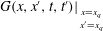 $G(x,x^{\prime },t,t^{\prime })|_{_{\begin{smallmatrix}x=x_{q}\\ x^{\prime }=x_{q}\\ \end{smallmatrix}}}$
. Details of the derivation can be found in appendix A. The resulting equations are
 $$\begin{eqnarray}(n_{1}\text{e}^{\text{i}{\it\Omega}_{m}{\it\tau}}-n_{0})\mathop{\sum }_{n=1}^{\infty }\left[\frac{G_{n}}{\text{i}({\it\omega}_{n}-{\it\Omega}_{m})}-\frac{G_{_{n}}^{\ast }}{\text{i}({\it\omega}_{_{n}}^{\ast }+{\it\Omega}_{m})}\right]=-\frac{2c^{2}}{K({\it\gamma}-1)},\end{eqnarray}$$
with
 $G_{n}$
given by (5.4), and
 $$\begin{eqnarray}\mathop{\sum }_{m=1}^{\infty }\left[u_{m}\frac{(-n_{1}\text{e}^{\text{i}{\it\Omega}_{m}{\it\tau}}+n_{0})}{\text{i}({\it\omega}_{n}-{\it\Omega}_{m})}+u_{m}^{\ast }\frac{(-n_{1}\text{e}^{-\text{i}{\it\Omega}_{m}^{\ast }{\it\tau}}+n_{0})}{\text{i}({\it\omega}_{n}+{\it\Omega}_{m}^{\ast })}\right]=\frac{\text{i}{\it\omega}_{n}{\it\varphi}_{o}+{{\it\varphi}^{\prime }}_{0}}{K({\it\gamma}-1)},\end{eqnarray}$$
as well as the complex conjugate of (5.8). Equation (5.7) is an equation for the frequencies
 ${\it\Omega}_{m}$
. Once this has been solved for
 ${\it\Omega}_{m}$
, the solution can be put into (5.8) and its complex conjugate to obtain the solution for the velocity amplitudes
 $u_{m}$
and
 $u_{m}^{\ast }$
.
Equations (5.7) and (5.8) show that the eigenmodes of the thermoacoustic system depend also on the parameters in the heat release model, in particular the heater power
 $K$
, the time lag
 ${\it\tau}$
and the coupling constants
 $n_{0}$
and
 $n_{1}$
. We call these eigenmodes the heat-driven modes of the system and their frequencies the heat-driven frequencies. Unless the feedback is missing,
 ${\it\Omega}_{m}$
and
 ${\it\omega}_{m}$
differ in both real and imaginary parts. The shift in real part is generally non-negligible (see results in § 8); this is a consequence of the thermoacoustic feedback. The imaginary part of
 ${\it\Omega}_{m}$
gives the stability behaviour of the heat-driven mode
 $m$
.
6 Stability maps
The stability behaviour of an individual mode will be determined as described in § 5.2, and the effect of the following control parameters will be examined:
-
(i) heat source position,
-
(ii) heater power and
-
(iii) tube length.
For each of these control parameters, we will examine the effect of the amplitude, using the amplitude-dependent expressions for
 ${\it\tau}$
,
 $n_{0}$
and
 $n_{1}$
, given in (4.4)–(4.6). The values of the constants
 ${\it\tau}_{0}$
,
 ${\it\tau}_{2}$
,
 $g_{0}$
and
 $g_{1}$
in these equations, which characterise the heat release, are kept fixed throughout the paper:
 ${\it\tau}_{0}=5\times 10^{-3}~\text{s}$
,
 ${\it\tau}_{2}=4.4\times 10^{-3}~\text{s}$
,
 $g_{0}=1.4$
and
 $g_{1}=0.3$
. We will limit our study to just the first mode,
 $m=1$
, and ignore the effect that any higher modes might have. We make this simplification because an isolated mode provides the most basic scenario and will give basic understanding. It will also allow us to separate the effects observed in a nonlinearly driven mode from those due to mode coupling (which we plan to study in a separate paper). Our results will be presented in the form of stability maps, depicting regions of stability and instability in the plane formed by the amplitude and one of the three control parameters listed above. We will show a large amplitude range, from zero to twice the mean flow velocity; this allows us to illustrate clearly the trends in stability behaviour as the amplitude increases. Of course, in most practical combustion systems, the maximum amplitude is below the value of the mean flow velocity.
We will consider two types of burner, characterised by different boundary conditions. One is a Rijke tube, which has open ends at
 $x=0$
(inlet) and
 $x=L$
(outlet), described by reflection coefficients
 $R_{0}=-1$
and
 $R_{L}=-1$
. The other burner is a quarter-wave resonator, with a closed end at
 $x=0$
and an open end at
 $x=L$
, described by reflection coefficients
 $R_{0}=1$
and
 $R_{L}=-1$
. These are idealised cases, where there are no losses of acoustic energy at the inlet or outlet. The reason for this choice of boundary conditions is to separate the effect of losses at the boundaries from the dependence of the stability behaviour on the control parameters under study.
6.1 Dependence on the heat source position
Figure 2 shows the stability map as a function of heat source position
 $x_{q}$
and amplitude
 $A/\bar{U}$
. The tube length is
 $L=2$
m, and the heater power is
 $K=3\times 10^{5}~\text{W}~\text{s}~\text{kg}^{-1}$
. The mean temperature is uniform throughout the tube,
 $\bar{T}_{1}=\bar{T}_{2}=304~\text{K}$
(room temperature), and the corresponding speed of sound is
 $c_{1}=c_{2}=350~\text{m}~\text{s}^{-1}$
. Figure 2(a) shows the results for the Rijke tube, and figure 2(b) shows those for the quarter-wave resonator. The grey/white areas denote, respectively, the regions in which the system is unstable/stable.
Stability maps depicting the dependence on heat source position
 $x_{q}$
and on (non-dimensional) amplitude
 $A/\bar{U}$
. Unstable regions are shaded in grey; stable regions are white. Within an unstable region, the growth rate
 $\text{Im}({\it\Omega}_{1})$
has a maximum at a point near the centre (not shown) and tends to zero as the edge of an instability region is approached. The mean temperature is uniform,
 $\bar{T}_{1}=\bar{T}_{2}=304~\text{K}$
. The combustor has length
 $L=2$
m and heater power
 $K=3\times 10^{5}~\text{W}~\text{s}~\text{kg}^{-1}$
.

A well-known feature of a Rijke tube is that it is unstable if the heat source is in the upstream half of the tube, and stable if it is in the downstream half (see e.g. § 6.2 in Dowling & Ffowcs Williams (Reference Dowling and Ffowcs Williams1983)). The position of this transition is determined by the point along the tube axis where the phase difference between pressure and velocity changes from
 ${\rm\pi}/2$
to
 $-{\rm\pi}/2$
. The time lag also plays a role. The stability behaviour described above occurs only for time lags in the range
 $0<{\it\tau}<T_{1}/2$
, where
 $T_{1}$
is the oscillation period of the first mode. For time lags in the range
 $T_{1}/2<{\it\tau}<T_{1}$
, the pattern is the other way round: the region of stability is in the upstream half, and instability in the downstream half (this can be shown with a simple analysis based on Rayleigh’s criterion (see e.g. Raun et al.
Reference Raun, Beckstead, Finlinson and Brooks1993)).
With these features in mind, it is straightforward to interpret the results shown in figure 2(a). The vertical transition line at
 $x_{q}=L/2$
is due to the phase jump between pressure and velocity. The alternating regions of stability and instability along the amplitude axis are due to the fact that the time lag
 ${\it\tau}$
increases with amplitude (see (4.4)). This increase is extensive: for small amplitudes,
 ${\it\tau}$
is a small fraction of the oscillation period, but it grows to more than twice the oscillation period for large amplitudes. Alternating regions of stability and instability have also been found by Heckl (Reference Heckl2015) for a matrix burner with an amplitude-dependent time lag.
The stability behaviour for the quarter-wave resonator is shown in figure 2(b). The vertical transition line is absent here because the phase difference between pressure and velocity is uniform along the whole length of the tube. There is a region of stability at low amplitudes, followed by a region of instability at higher amplitudes. As in the case of the Rijke tube, this is due to the amplitude dependence of the time lag. These regions are wider along the amplitude axis here because the oscillation period of the first mode is greater.
If the system is at a point in an unstable (grey) zone in figure 2(a) or 2(b), the perturbation amplitude grows until the border with a stable zone is reached. On the other hand, if the system is in a stable (white) zone, the amplitude drops down to the border with the neighbouring unstable zone.
The curved interfaces along the top of the grey zones represent stable limit cycles: any small variation of
 $A/\bar{U}$
from the interface will bring the perturbation back to the original amplitude. The basin of attraction for such a limit cycle is the grey area below it and the white area above it. The curved interfaces along the bottom of the grey zones represent the basin boundaries (Strogatz Reference Strogatz1994).
It is worth reiterating that we only present results for the ideal case where acoustic losses are zero. Losses have a stabilising effect, so, if they are taken into account, the regions of stability become larger at the expense of regions of instability. This explains, for example, our prediction (contrary to experimental observation) that the Rijke tube is unstable, even when the heater is located directly at the upstream tube end.
The stability map for the Rijke tube becomes more fragmented if the mean temperature is increased. Figure 3 shows an example for
 $\bar{T}_{1}=\bar{T}_{2}=380~\text{K}$
and
 $c_{1}=c_{2}=390~\text{m}~\text{s}^{-1}$
. All other parameters are the same as for figure 2. The stable zone on the bottom right in figure 2(a) has become divided into two parts: one close to the transition line and one close to the outlet (see figure 3
a). We will show in § 9 that this feature can be a cause of hysteresis when the heat source is moved along the tube axis. The map for the quarter-wave resonator shows very little change (see figure 3
b).
Stability maps depicting the dependence on heat source position
 $x_{q}$
and on (non-dimensional) amplitude
 $A/\bar{U}$
. Unstable regions are shaded in grey; stable regions are white. The mean temperature is uniform,
 $\bar{T}_{1}=\bar{T}_{2}=380~\text{K}$
, which is higher than in figure 2. The combustor has length
 $L=2$
m and heater power
 $K=3\times 10^{5}~\text{W}~\text{s}~\text{kg}^{-1}$
.

A similar effect is observed if a temperature jump is introduced. Figure 4 shows a case where
 $\bar{T}_{1}=304~\text{K}$
,
 $\bar{T}_{2}=460~\text{K}$
,
 $c_{1}=350~\text{m}~\text{s}^{-1}$
and
 $c_{2}=430~\text{m}~\text{s}^{-1}$
. The vertical transition line present in figures 2(a) and 3(a) at
 $L/2$
has moved towards the inlet in figure 4(a). This is due to the discontinuity in mean temperature: the speed of sound jumps from a lower to a higher value, and with it jumps the wavelength. This leads to a shift in the position where the phase difference between pressure and velocity changes from
 ${\rm\pi}/2$
to
 $-{\rm\pi}/2$
. There are no qualitative changes in the map of the quarter-wave resonator (see figure 4
b).
Stability maps depicting the dependence on heat source position
 $x_{q}$
and on (non-dimensional) amplitude
 $A/\bar{U}$
. Unstable regions are shaded in grey; stable regions are white. The mean temperature jumps at
 $x_{q}$
from
 $\bar{T}_{1}=304~\text{K}$
to
 $\bar{T}_{2}=460~\text{K}$
. The combustor has length
 $L=2$
m and heater power
 $K=3\times 10^{5}~\text{W}~\text{s}~\text{kg}^{-1}$
.

The effect of an increase or jump in mean temperature can be explained as follows. An increase in mean temperature leads to an increase in the eigenfrequencies and a decrease in the corresponding oscillation periods (
 $T_{1}$
for the first mode). As we mentioned earlier in this section, there is a critical time lag at
 ${\it\tau}=T_{1}/2$
; there a switch occurs from stability to instability (or vice versa). The fragmentation of the stability maps in figures 3 and 4 is due to the reduction of the critical time lag, which in turn is due to the increase in mean temperature.
6.2 Dependence on tube length
In some combustors it is possible to tune the tube by varying its length (see e.g. Evesque, Dowling & Annaswamy Reference Evesque, Dowling and Annaswamy2003; Noiray et al.
Reference Noiray, Durox, Schuller and Candel2008). We therefore consider the tube length
 $L$
as control parameter in our study, and present stability maps to show its effects in the range
 $L=0.3,\ldots ,2~\text{m}$
. The heat source is kept fixed at position
 $x_{q}=0.1~\text{m}$
. The parameters characterising the (amplitude-dependent) heat release rate have the same values as in § 6.1. The mean temperature is 380 K and is uniform. Figure 5(a) shows the stability map for the Rijke tube, while figure 5(b) shows that of the quarter-wave resonator.
Stability maps depicting the dependence on tube length
 $L$
and on (non-dimensional) amplitude
 $A/\bar{U}$
. Unstable regions are shaded in grey; stable regions are white. The mean temperature is uniform
 $\bar{T}_{1}=\bar{T}_{2}=380~\text{K}$
. The heat source is located at
 $x_{q}=0.10~\text{m}$
; the heater power is
 $K=3\times 10^{5}~\text{W}~\text{s}~\text{kg}^{-1}$
.

We observe that for both types of tube the stable/unstable zones have the shape of a curved band, whose thickness and curvature change smoothly with the tube length. There are more stability/instability bands in the map for the Rijke tube than in the map for the quarter-wave resonator.
The stability map shown in figure 5(b) corresponds directly to that found experimentally by Noiray et al. (Reference Noiray, Durox, Schuller and Candel2008) for a quarter-wave resonator with a flame that releases heat as described in § 4. The qualitative agreement is good at low amplitudes, but not for amplitudes above approximately 0.2. Put in nonlinear dynamics terms, we predict the subcritical Hopf bifurcation point correctly, but fail to capture the fold point. This discrepancy was explained by Heckl (Reference Heckl2015) and is not important for the purposes of the current paper. (It is due to the fact that our description of the heat release rate effectively ignores the low-pass behaviour of the measured FDF).
6.3 Dependence on the heater power
The constant
 $K$
in our model for the heat release (see (4.2)) is the heater power (per mass flow rate); we treat it as an independent parameter. In the following we will investigate how it influences the stability behaviour of the Rijke tube and the quarter-wave resonator. The tube length is fixed,
 $L=2~\text{m}$
. The parameters characterising the (amplitude-dependent) heat release rate have the same values as in § 6.1.
We now take into account that the jump in mean temperature is caused by the heat source and is given by (Sonntag, Borgnakke & van Wylen Reference Sonntag, Borgnakke and van Wylen2003, § 5.6)
 $$\begin{eqnarray}{\rm\Delta}T=\frac{\bar{Q}}{c_{p}S\bar{U}\bar{{\it\rho}}},\end{eqnarray}$$
where
 $\bar{Q}$
is the mean heat release, related to
 $K$
by (4.3), and
 $c_{p}$
is the heat capacity for constant pressure. Two different heat source positions will be considered,
 $x_{q}=0.10~\text{m}$
and
 $x_{q}=0.50~\text{m}$
, in order to have a complete overview of the stability changes induced by varying
 $K$
.
The maps for
 $x_{q}=0.10~\text{m}$
are shown in figure 6, and the maps for
 $x_{q}=0.50~\text{m}$
are shown in figure 7. Panels (a) of these figures are for the Rijke tube and panels (b) are for the quarter-wave resonator. The regions of stability/instability tend to have the shape of bands, sloping downwards towards the right.
Stability maps depicting the dependence on the heater power
 $K$
and on (non-dimensional) amplitude
 $A/\bar{U}$
. Unstable regions are shaded in grey; stable regions are white. The mean temperature jumps at
 $x_{q}$
from
 $\bar{T}_{1}=304~\text{K}$
to
 $\bar{T}_{2}=\bar{T}_{1}+{\rm\Delta}T$
, where the temperature increase
 ${\rm\Delta}T$
depends on the heater power as given by (6.1), with
 $c_{p}=1010~\text{J}~\text{kg}^{-1}~\text{K}^{-1}$
. The heat source is located at
 $x_{q}=0.10~\text{m}$
; the combustor has length
 $L=2$
m.

Stability maps depicting the dependence on the heater power
 $K$
and on (non-dimensional) amplitude
 $A/\bar{U}$
. Unstable regions are shaded in grey; stable regions are white. The mean temperature jumps at
 $x_{q}$
from
 $\bar{T}_{1}=304~\text{K}$
to
 $\bar{T}_{2}=\bar{T}_{1}+{\rm\Delta}T$
, where the temperature increase
 ${\rm\Delta}T$
depends on the heater power as given by (6.1), with
 $c_{p}=1010~\text{J}~\text{kg}^{-1}~\text{K}^{-1}$
. The heat source is located further downstream than in figure 6, at
 $x_{q}=0.50~\text{m}$
; the combustor has length
 $L=2$
m.

We observe that the quarter-wave resonator tends to be more unstable for higher
 $K$
values. Comparing figures 6(b) and 7(b), we also observe that the heat source position makes very little difference. This is as expected from § 6.1, where we found that the stability behaviour of the quarter-wave resonator has only a weak dependence on the heat source position.
For the Rijke tube, there are again more regions of stability/instability than for the quarter-wave resonator, and, as a consequence, more variation in the stability behaviour can be expected. We illustrate this by comparing figures 6(a) and 7(a). An increase in heater power tends to destabilise the system (for small amplitudes) if the heat source is close to the upstream end (see figure 6
a, where
 $x_{q}=0.1~\text{m}$
), but not if it is a little further downstream (see figure 7
a, where
 $x_{q}=0.5~\text{m}$
).
Gopalakrishnan & Sujith (Reference Gopalakrishnan and Sujith2014) have performed experimental studies, where they used the heater power, and also the heater position, in a Rijke tube as control parameter and found a subcritical Hopf bifurcation, as well as a fold bifurcation. The Hopf bifurcation is predicted correctly by our approach, but the fold point is missing. This discrepancy is similar to that observed in § 6.2 and is due to the same reason: we have used a generic FDF, and not one that accurately describes the FDF in the experimental set-up. In addition, losses are not taken into account, as discussed in § 6.1.
7 Frequency shift
As we pointed out in § 5.2, thermoacoustic feedback causes a shift in the modal frequencies, i.e. the real part of
 ${\it\omega}_{m}$
generally differs from that of
 ${\it\Omega}_{m}$
. In the following we will show that the shift depends on the system parameters and on the perturbation amplitude. We again consider mode
 $m=1$
of the Rijke tube and of the quarter-wave resonator, and display the frequency values by a contour map in the plane of the parameters
 $K$
and
 $A/\bar{U}$
. Figure 8 shows the real part of
 ${\it\omega}_{1}$
; this is obviously constant with respect to amplitude. The real part of
 ${\it\Omega}_{1}$
, however, shown in figure 9, is clearly dependent on amplitude, and this becomes more pronounced with increasing heater power.
Contour plots showing the natural frequency
 $\text{Re}\,{\it\omega}_{1}$
as a function of heater power
 $K$
and the (non-dimensional) amplitude
 $A/\bar{U}$
. The mean temperature jumps at
 $x_{q}$
from
 $\bar{T}_{1}=304~\text{K}$
to
 $\bar{T}_{2}=\bar{T}_{1}+{\rm\Delta}T$
, where the temperature increase
 ${\rm\Delta}T$
depends on the heater power as given by (6.1), with
 $c_{p}=1010~\text{J}~\text{kg}^{-1}~\text{K}^{-1}$
. The heat source is located at
 $x_{q}=0.10~\text{m}$
; the combustor has length
 $L=2$
m.

Contour plots showing the heat-driven frequency
 $\text{Re}\,{\it\Omega}_{1}$
as a function of heater power
 $K$
and the (non-dimensional) amplitude
 $A/\bar{U}$
. The mean temperature jumps at
 $x_{q}$
from
 $\bar{T}_{1}=304~\text{K}$
to
 $\bar{T}_{2}=\bar{T}_{1}+{\rm\Delta}T$
, where the temperature increase
 ${\rm\Delta}T$
depends on the heater power as given by (6.1), with
 $c_{p}=1010~\text{J}~\text{kg}^{-1}~\text{K}^{-1}$
. The heat source is located at
 $x_{q}=0.10~\text{m}$
; the combustor has length
 $L=2$
m.

Comparing the contour plots for
 $\text{Re}\,{\it\omega}_{1}$
and
 $\text{Re}\,{\it\Omega}_{1}$
, we see that the frequency shift can be positive, negative or zero. The points where
 ${\it\Omega}_{1}={\it\omega}_{1}$
lie on a curve (not shown here), which is unrelated to any of the curved interfaces between regions of stability and instability in figure 6. The frequency shift is caused by the thermoacoustic feedback. Here, the thermoacoustic feedback is amplitude-dependent (through the heat release law described in § 4), and therefore the heat-driven frequencies become amplitude-dependent. The shifts in the real part (oscillation frequencies) are not as dramatic as the shifts in the imaginary part (growth rate), but they are nevertheless important: they are particularly relevant for elaborate combustion systems, which have components that are prone to resonance excitation.
8 Validation
We validate our stability maps with the iterative calculation of the time evolution described in § 5.1. Starting from a specific point in the map, we expect an oscillation whose amplitude decreases/increases with time if the starting point was in a stable/unstable zone. Likewise, we expect an oscillation with constant amplitude if the starting point was at an interface representing a stable limit cycle.
We performed the validation for many points in the stability map and for many parameter combinations (
 $x_{q},L,K$
), and in every case the results from the time evolution confirmed the results in the map. An example is shown in figure 10(a), where the time history of the acoustic velocity in a Rijke tube is shown; the starting point of the iteration was the point
 $x_{q}=1.47~\text{m}$
,
 $A/\bar{U}=0.01$
in the stability map shown in figure 4(a). The time history clearly shows the amplitude growth after the initial velocity perturbation, followed by the limit cycle. This corresponds to a point in the stability map undergoing a vertical shift, until it reaches the upper boundary of the unstable zone.
The time evolution also gives the frequency of the heat-driven oscillation. In order to illustrate this, we calculated the frequency spectrum associated with figure 10(a); this is shown in figure 10(b). There is a sharp peak at
 $565~\text{s}^{-1}$
; this value agrees with the analytical result
 $\text{Re}\,{\it\Omega}_{1}=565~\text{s}^{-1}$
found from (5.7).
The corresponding natural frequency, i.e. the frequency without thermoacoustic feedback, is distinctly different:
 $\text{Re}\,{\it\omega}_{1}=596~\text{s}^{-1}$
. This is an example of the frequency shift resulting from thermoacoustic feedback, discussed in § 7.
Acoustic velocity in the Rijke tube: (a) the time evolution, and (b) the frequency spectrum. The heat source is located at
 $x_{q}=1.47~\text{m}$
, and the initial perturbation amplitude is
 $A/\bar{U}=0.01$
. The other parameters are as in figure 4: the mean temperature jumps at
 $x_{q}$
from
 $\bar{T}_{1}=304~\text{K}$
to
 $\bar{T}_{2}=460~\text{K}$
; the combustor has length
 $L=2$
m and heater power
 $K=3\times 10^{5}~\text{W}~\text{s}~\text{kg}^{-1}$
.

9 Hysteresis
Some features in the stability maps shown in §§ 6.1–6.3 indicate that there is potential for hysteretic behaviour when a certain control parameter is varied. We will study this now in more detail, based on the iterative calculation of time histories as described in § 5.1. Two control parameters will be considered: the heat source position
 $x_{q}$
and the tube length
 $L$
. We will vary them by increasing and subsequently decreasing them (or vice versa).
9.1 Heat source position as control parameter
We will illustrate the procedure for the case where we move the heat source from the inlet to the outlet and then back to the inlet:
-
(1) We pick a heat source position close to the inlet, e.g. the position
 $x_{q1}=0.01~\text{m}$
, and a small initial perturbation amplitude, e.g.
$A_{0}/\bar{U}=0.01$
. We then calculate the time evolution for many cycles until the amplitude reaches saturation (in general 10 s will be sufficient). We register the amplitude
$A_{1}/\bar{U}$
of the perturbation at saturation.
-
(2) We move the heat source position to the right by a small distance
${\rm\Delta}x$
and continue to calculate the time evolution for the new position,
$x_{q2}=x_{q1}+{\rm\Delta}x$
. The initial perturbation amplitude for this calculation is
$A_{1}/\bar{U}$
. Once saturation is reached, we again register the velocity amplitude
$A_{2}/\bar{U}$
of the perturbation at saturation. -
(3) We repeat step 2 until the heat source position reaches the outlet of the tube, and record the saturation amplitude for each position, thus obtaining an array of
$N$
amplitude values. -
(4) Next we repeat the calculation, steps 1–3, but move the heat source in the opposite direction, from the outlet to the inlet. At the point of reversal, the amplitude is equal to the
$A_{N}/\bar{U}$
value obtained for the last heater position
$x_{N}$
of step 3. We proceed with the iteration for heater positions
$x_{qn}=x_{qn-1}-{\rm\Delta}x$
, recording
$A_{n}/\bar{U}$
at each step.




The same procedure can be applied when moving from an arbitrary starting point
 $x_{i}$
to a point
 $x_{j}$
, and then back from
 $x_{j}$
to
 $x_{i}$
. Various initial values and control parameter ranges will be chosen in order to establish whether hysteretic behaviour occurs.
A case is shown in figure 11, which corresponds to the stability map in figure 4(a). The area shaded in grey shows the region of instability on the bottom right of figure 4(a) (note that here we display only a part of the stability maps in § 6.1:
 $x_{q}=0.9,\ldots ,2~\text{m}$
,
 $A/\bar{U}=0,\ldots ,1.6$
). The time history calculation started with the heat source at the outlet end of the tube, and the source was then moved towards the inlet end. The dashed green line in figure 11 shows the path (right to left) in the stability map. Just before reaching the point
 $x_{q}=0.9$
m, the movement of the source is reversed, from left to right; the corresponding path is shown by the solid blue line. The iteration calculating the time history simply continues at the point of reversal, i.e. no new initial conditions are introduced.
Hysteresis in the stability map of the Rijke tube with heater position
 $x_{q}$
as control parameter. The map is the bottom right section of the map in figure 4(a) and has the same parameters (
 $\bar{T_{1}}=304$
K,
 $\bar{T_{2}}=460$
K,
 $L=2$
m,
 $K=3\times 10^{5}~\text{W}~\text{s}~\text{kg}^{-1}$
). Stable regions (white) are labelled
 $Z_{1}$
,
 $Z_{3}$
and
 $Z_{4}$
; the unstable region (grey) is
 $Z_{2}$
. The dashed green line shows the left-to-right path (indicated by green arrows); the solid blue line shows the right-to-left path (indicated by blue arrows). Hysteresis is indicated by the green/blue arrows when moving the heat source from the outlet to
 $x_{q}=0.9$
m (green arrows) and then back to the outlet (blue arrows).

The paths labelled by the green and blue arrows in the stability map are clearly different, indicating that hysteresis is present. We now explore this in more detail by looking at the individual regions of stability and instability as they are crossed or skirted by the paths. If we start from a point in the stable region
 $Z_{3}$
and move the heat source backwards from the outlet, the system is stable until
 $x_{q}=1.49~\text{m}$
. After this point the system enters the unstable region
 $Z_{2}$
. The amplitude then grows until it reaches the interface with zone
 $Z_{4}$
. This represents a stable limit cycle and further decrease of
 $x_{q}$
leads the system along this interface. However, if we now reverse the direction of the heat source before reaching the vertical transition line at
 $x_{q}=0.90~\text{m}$
, and move it back towards the outlet, the system will not re-enter the stable zone
 $Z_{3}$
but will continue to follow the interface until the outlet, performing stable limit cycle oscillations. The same kind of behaviour is observed if the heat source is first moved forwards, starting from a point in the stable region
 $Z_{1}$
, and then backwards towards the inlet before reaching
 $x_{q}=1.49~\text{m}$
. This is in exact qualitative agreement with the experimental observations by Gopalakrishnan & Sujith (Reference Gopalakrishnan and Sujith2014). There are disagreements with other aspects of their observations, in particular the fold bifurcation observed by them is not predicted. This discrepancy is due to our choice of heat release law, which is probably dissimilar from the one in their experiment.
We note that the size of the zones
 $Z_{1}$
and
 $Z_{3}$
determines the extent of the hysteresis. This can be manipulated by varying the heater power
 $K$
. In fact it is possible, by suitable choice of
 $K$
, to suppress hysteresis altogether, without restricting the range of positions
 $x_{q}$
.
9.2 Tube length as control parameter
We can apply the four-step procedure described in § 9.1 to study the variation of the tube length, and increase/decrease
 $L$
by small steps
 ${\rm\Delta}L$
. The results are shown in figure 12(a,b) and correspond directly to figure 5(a,b). Again, the areas shaded in grey indicate the regions of instability, the solid blue lines mark the forward direction (left to right), and the dashed green lines mark the backward direction (right to left).
Hysteresis in the stability map of the Rijke tube (a) and quarter-wave resonator (b) with combustor length
 $L$
as control parameter. The maps are the same as in figure 5 and have the same parameters (
 $T_{1}=T_{2}=380$
K,
 $x_{q}=0.10$
m,
 $K=3\times 10^{5}~\text{W}~\text{s}~\text{kg}^{-1}$
). The dashed green line shows the backward path (indicated by green arrows); the solid blue line shows the forward path (indicated by blue arrows).

We note that if we decrease the tube length from
 $L=2~\text{m}$
to the stable interval just beyond
 $L=0.5~\text{m}$
, and subsequently increase it again from there to
 $L=2~\text{m}$
, the path followed by the system in the stability map is not the same. A wide hysteresis is present, both for the Rijke tube and for the quarter-wave resonator. However, we observe from the stability maps that it is possible to avoid hysteresis by limiting the tube length to the range
 $L=1~\text{m},\ldots ,2~\text{m}$
(assuming the initial perturbation is small).
The same type of calculation can be made for decreasing/increasing the heater power
 $K$
, instead of the tube length, and the results are quite similar (not shown here). Again, hysteresis can be avoided by restricting the
 $K$
values to a range that keeps the path in the first stable zone of the stability map. We note that for the case shown in the map of figure 7(a) for a Rijke tube (with
 $x_{q}=0.5~\text{m}$
and
 $L=2~\text{m}$
), hysteresis cannot occur.
A thermoacoustic system that is linearly stable can be launched into a state where it performs self-sustained oscillations if it is excited by a large enough impulse. This is another nonlinear phenomenon and has been observed in practical combustion systems (see e.g. Juniper Reference Juniper2011). Our predicted stability maps give direct information on the amplitude levels that trigger self-sustained oscillations, and this information agrees qualitatively with the predictions by Juniper.
10 Conclusions
We have described a Green’s function approach to model thermoacoustic oscillations and hysteresis in two 1D systems: a Rijke tube and a quarter-wave resonator. The stability analysis was performed in two ways:
-
(1) Derivation of a characteristic equation for the individual modes in the presence of thermoacoustic feedback. This equation was solved with the Newton–Raphson root-finding algorithm to obtain the complex heat-driven frequencies; their real part gives the frequency of the oscillation, and the imaginary part gives the stability behaviour. This method allows the identification of the attractors of the system (limit cycles) as a function of different parameters. It also gives the triggering amplitudes, as well as the frequency shift induced by thermoacoustic feedback.
-
(2) Derivation of an integral equation governing the time history of the acoustic field. This was solved by numerical iteration to give explicit information on any hysteresis that may be present.
Ours is the first time-domain study where a system parameter is varied during the calculation of the time history. We have shown that hysteresis occurs if any of the three control parameters (heat source position, tube length and heater power) is increased and subsequently decreased. For the heat source position, our hysteresis prediction is coherent with the experimental observations on a horizontal Rijke tube with low-Mach-number flow. Our work thus represents a major step towards developing analytical models for experiments where a system parameter is varied and nonlinear transitions are observed.
The Green’s function is a linear concept. One may therefore question our approach to tackle nonlinear problems with it. The explanation lies in the source of the nonlinearity, which is in the thermoacoustic feedback. The acoustic waves themselves are regarded as linear, and it is therefore justified to describe them with a Green’s function.
Our approach can be extended in various ways:
-
(1) Extension in terms of combustor geometry. In this study, we have considered a basic combustor geometry: a uniform tube with open or closed ends, and a mean temperature inside the tube that was either uniform or piecewise uniform (cold upstream and hot downstream of the heat source). Our model can be extended so that it applies to a typical laboratory burner, which features specific end conditions, a localised change in cross-sectional area, and/or a localised obstacle blocking the flow.
-
(2) Extension with a network approach. Our method can be extended further to more complicated geometries by modelling each element of the combustion system. This can be done by using experimental data or by performing a few short CFD simulations. Once the response function of each element is known, the Green’s function method can then be used for a parametric study.
-
(3) Extension in terms of the model for the heat source. For the thermoacoustic feedback, we have assumed an amplitude-dependent relationship between the heat release rate and the flow velocity (including a time-lag term and a direct-feedback term). Our approach is not limited to such a quasi-linear heat release law, but works more generally, as long as the heat release rate is given as a function (linear or nonlinear) of the acoustic velocity. This function might come from an analytical model for the flame, from experiments, or from numerical simulations.
-
(4) Extension to multiple modes. In this article we have considered the case where the modes do not interact and a single mode can be treated in isolation. Our Green’s function method can be extended to include several interacting modes, and this will be treated in a future paper.
-
(5) Extension to include losses. In this study, we have presented stability predictions for the case where there are no acoustic losses. Losses at the combustor ends can be simulated with the current model by suitable choice of the reflection coefficients
$R_{0}$
and
$R_{L}$
. Our predictions for lossy ends (not shown in this paper) confirm the general expectation that losses have a stabilising effect, reducing the size of the unstable zones in the stability maps.


In order to operate a combustion system safely, it is necessary to know its stability boundaries for the conditions under which it is expected to operate. Our Green’s function approach provides this kind of information fast and with a minimum of numerical effort: it takes just a few seconds (on a standard PC or laptop) to produce a stability map, while a time history takes between 30 s and 10 min to calculate, depending on the number of iteration steps required. Although our predictions involve a degree of approximation, they are nevertheless very useful for guiding experimental and numerical studies: experiments to find the stability boundaries based on trial and error are risky and expensive. With a rough idea where these boundaries are, it is much easier to find them and determine them accurately. Finding the stability boundaries from a numerical code (such as CFD, LES or DNS) requires a lot computational effort. Our approach could complement simulations, which are not suited for parameter studies, by providing rough information on the relevant parameter ranges.
The Green’s function is a mathematical tool, but it also has a very concrete physical meaning: it is the response of a burner to an impulse excitation. This physical interpretation is very valuable. We have exploited it in this paper to describe a burner in terms of actual physical modes (with and without thermoacoustic feedback), rather than in terms of the idealised modes that tend to be used in connection with the Galerkin method. The physical insight gained with our approach is fundamental for the understanding and control of thermoacoustic feedback in combustors.
Other types of instability involving a resonator can be modelled by our Green’s function approach. This has been done for friction-driven oscillations, such as the bowed string (McIntyre & Woodhouse Reference Mcintyre and Woodhouse1979) and curve squeal (Heckl Reference Heckl2000). Friction-driven oscillations are an instability generated by the nonlinear feedback between the friction force and the relative velocity of two solid bodies in contact. We are optimistic that there are further cases of unstable oscillations that would be amenable to modelling with our approach.
Acknowledgements
The presented work is part of the Marie Curie Initial Training Network ‘Thermoacoustic and Aeroacoustic Nonlinearities in Green combustors with Orifice structures’ (TANGO). We gratefully acknowledge the financial support from the European Commission under call FP7-PEOPLE-ITN-2012.
Appendix A. Derivation of (5.7) and (5.8)
The equations for the heat-driven frequencies
 ${\it\Omega}_{m}$
and amplitudes
 $u_{m}$
can be obtained with a procedure first used by Heckl (Reference Heckl2000) to analyse a friction-driven wheel. We combine the equations (4.2) and (5.6) in order to obtain a modal expression for the heat release:
 $$\begin{eqnarray}q(t)=K\left[n_{1}\mathop{\sum }_{m=1}^{\infty }(u_{m}\text{e}^{-\text{i}{\it\Omega}_{m}(t-{\it\tau})}+u_{m}^{\ast }\text{e}^{\text{i}{\it\Omega}_{m}^{\ast }(t-{\it\tau})})-n_{0}\mathop{\sum }_{m=1}^{\infty }(u_{m}\text{e}^{-\text{i}{\it\Omega}_{m}t}+u_{m}^{\ast }\text{e}^{\text{i}{\it\Omega}_{m}^{\ast }t})\right].\end{eqnarray}$$
Also, we rewrite the integral governing equation (3.4), using the modal expression (2.2) for the Green’s function,
 $$\begin{eqnarray}\displaystyle u_{q}(t) & = & \displaystyle -\frac{{\it\gamma}-1}{2c^{2}}\int _{t^{\prime }=0}^{t}q(t^{\prime })\mathop{\sum }_{n=1}^{\infty }(G_{n}\text{e}^{-\text{i}{\it\omega}_{n}t}+G_{n}^{\ast }\text{e}^{\text{i}{\it\omega}_{n}^{\ast }t})\,\text{d}t^{\prime }\nonumber\\ \displaystyle & & \displaystyle +\,\frac{1}{2c^{2}}\mathop{\sum }_{n=1}^{\infty }[(\text{i}{\it\omega}_{n}{\it\varphi}_{0}+{{\it\varphi}^{\prime }}_{0})G_{n}\text{e}^{-\text{i}{\it\omega}_{n}t}+(-\text{i}{\it\omega}_{n}^{\ast }{\it\varphi}_{0}+{{\it\varphi}^{\prime }}_{0})G_{n}^{\ast }\text{e}^{\text{i}{\it\omega}_{n}^{\ast }t}],\end{eqnarray}$$
where we have used the abbreviation (5.4). We then substitute in (A 2) for
 $q(t)$
with (A 1), and for
 $u_{q}(t)$
with (5.6). This leads to the following equation:
 $$\begin{eqnarray}\displaystyle & & \displaystyle \mathop{\sum }_{m=1}^{\infty }(u_{m}\text{e}^{-\text{i}{\it\Omega}_{m}t}+u_{m}^{\ast }\text{e}^{\text{i}{\it\Omega}_{m}^{\ast }t})\nonumber\\ \displaystyle & & \displaystyle \quad =\frac{Kn_{0}({\it\gamma}-1)}{2c^{2}}\int _{t^{\prime }=0}^{t}\mathop{\sum }_{n=1}^{\infty }(G_{n}\text{e}^{-\text{i}{\it\omega}_{n}(t-t^{\prime })}+G_{n}^{\ast }\text{e}^{\text{i}{\it\omega}_{n}^{\ast }(t-t^{\prime })})\mathop{\sum }_{m=1}^{\infty }(u_{m}\text{e}^{-\text{i}{\it\Omega}_{m}t^{\prime }}+u_{m}^{\ast }\text{e}^{\text{i}{\it\Omega}_{m}^{\ast }t^{\prime }})\,\text{d}t^{\prime }\nonumber\\ \displaystyle & & \displaystyle \qquad -\,\frac{Kn_{1}({\it\gamma}-1)}{2c^{2}}\int _{t^{\prime }=0}^{t}\mathop{\sum }_{n=1}^{\infty }(G_{n}\text{e}^{-\text{i}{\it\omega}_{n}(t-t^{\prime })}+G_{n}^{\ast }\text{e}^{\text{i}{\it\omega}_{n}^{\ast }(t-t^{\prime })})\nonumber\\ \displaystyle & & \displaystyle \qquad \times \,\mathop{\sum }_{m=1}^{\infty }(u_{m}\text{e}^{-\text{i}{\it\Omega}_{m}(t^{\prime }-{\it\tau})}+u_{m}^{\ast }\text{e}^{\text{i}{\it\Omega}_{m}^{\ast }(t^{\prime }-{\it\tau})})\,\text{d}t^{\prime }\nonumber\\ \displaystyle & & \displaystyle \qquad +\,\frac{1}{2c^{2}}\mathop{\sum }_{n=1}^{\infty }[(\text{i}{\it\omega}_{n}{\it\varphi}_{0}+{{\it\varphi}^{\prime }}_{0})G_{n}\text{e}^{-\text{i}{\it\omega}_{n}t}+(-\text{i}{\it\omega}_{n}^{\ast }{\it\varphi}_{0}+{{\it\varphi}^{\prime }}_{0})G_{n}^{\ast }\text{e}^{\text{i}{\it\omega}_{n}^{\ast }t}].\end{eqnarray}$$
We distinguish between the heat-driven mode, which has frequency
 ${\it\Omega}_{m}$
and amplitude
 $u_{m}$
, and the natural mode, which has frequency
 ${\it\omega}_{n}$
and amplitude
 $G_{n}$
(
 $x$
derivative).
The two integrals on the right-hand side of (A 3) can be combined and written more compactly as
 $$\begin{eqnarray}\displaystyle & & \displaystyle -\frac{K({\it\gamma}-1)}{2c^{2}}\int _{t^{\prime }=0}^{t}\left\{\mathop{\sum }_{m,n} [G_{n}u_{m}\text{e}^{\text{i}({\it\omega}_{n}-{\it\Omega}_{m})t^{\prime }-i{\it\omega}_{n}t}(n_{1}\text{e}^{\text{i}{\it\Omega}_{m}{\it\tau}}-n_{0})\right.\nonumber\\ \displaystyle & & \displaystyle \quad +\,G_{n}^{\ast }u_{m}\text{e}^{-\text{i}({\it\omega}_{n}^{\ast }+{\it\Omega}_{m})t^{\prime }+\text{i}{\it\omega}_{n}^{\ast }t}(n_{1}\text{e}^{\text{i}{\it\Omega}_{m}{\it\tau}}-n_{0})+G_{n}u_{m}^{\ast }\text{e}^{\text{i}({\it\omega}_{n}+{\it\Omega}_{m}^{\ast })t^{\prime }-\text{i}{\it\omega}_{n}t}(n_{1}\text{e}^{-\text{i}{\it\Omega}_{m}^{\ast }{\it\tau}}-n_{0})\nonumber\\ \displaystyle & & \displaystyle \quad \left.+\,G_{n}^{\ast }u_{m}^{\ast }\text{e}^{\text{i}({\it\Omega}_{m}^{\ast }-{\it\omega}_{n}^{\ast })t^{\prime }+\text{i}{\it\omega}_{n}^{\ast }t}(n_{1}\text{e}^{-\text{i}{\it\Omega}_{m}^{\ast }{\it\tau}}-n_{0})]\vphantom{\mathop{\sum }_{m,n}}\right\}\,\text{d}t^{\prime }.\end{eqnarray}$$
After evaluation of the integral in expression (A 4), this becomes
 $$\begin{eqnarray}\displaystyle & & \displaystyle \frac{K({\it\gamma}-1)}{2c^{2}}\mathop{\sum }_{m,n}\left\{(-n_{1}\text{e}^{\text{i}{\it\Omega}_{m}{\it\tau}}+n_{0})\left[G_{n}u_{m}\frac{\text{e}^{\text{i}({\it\omega}_{n}-{\it\Omega}_{m})t}-1}{\text{i}({\it\omega}_{n}-{\it\Omega}_{m})}\text{e}^{-\text{i}{\it\omega}_{n}t}+G_{n}^{\ast }u_{m}\frac{\text{e}^{\text{i}(-{\it\omega}_{n}^{\ast }-{\it\Omega}_{m})t}-1}{\text{i}(-{\it\omega}_{n}^{\ast }-{\it\Omega}_{m})}\text{e}^{-\text{i}{\it\omega}_{n}^{\ast }t}\right]\right.\nonumber\\ \displaystyle & & \displaystyle \quad \left.+\,(-n_{1}\text{e}^{-\text{i}{\it\Omega}_{m}^{\ast }{\it\tau}}+n_{0})\left[G_{n}u_{m}^{\ast }\frac{\text{e}^{\text{i}({\it\omega}_{n}+{\it\Omega}_{m}^{\ast })t}-1}{\text{i}({\it\omega}_{n}+{\it\Omega}_{m}^{\ast })}\text{e}^{-\text{i}{\it\omega}_{n}t}+G_{n}^{\ast }u_{m}^{\ast }\frac{\text{e}^{\text{i}(-{\it\omega}_{n}^{\ast }+{\it\Omega}_{m}^{\ast })t}-1}{\text{i}(-{\it\omega}_{n}^{\ast }+{\it\Omega}_{m}^{\ast })}\text{e}^{\text{i}{\it\omega}_{n}^{\ast }t}\right]\right\}.\end{eqnarray}$$
We insert this into (A 3) and rearrange to group the terms with factors
 $u_{m}\text{e}^{-\text{i}{\it\Omega}_{m}t}$
,
 $u_{m}^{\ast }\text{e}^{\text{i}{\it\Omega}_{m}^{\ast }t}$
,
 $G_{n}\text{e}^{-\text{i}{\it\omega}_{n}t}$
and
 $G_{n}^{\ast }\text{e}^{\text{i}{\it\omega}_{n}^{\ast }t}$
. The result is
 $$\begin{eqnarray}\displaystyle & & \displaystyle \mathop{\sum }_{m=1}^{\infty }(u_{m}\text{e}^{-\text{i}{\it\Omega}_{m}t}+u_{m}^{\ast }\text{e}^{\text{i}{\it\Omega}_{m}^{\ast }t})\nonumber\\ \displaystyle & & \displaystyle \quad =\mathop{\sum }_{m=1}^{\infty }u_{m}\text{e}^{-\text{i}{\it\Omega}_{m}t}\frac{K({\it\gamma}-1)}{2c^{2}}(-n_{1}\text{e}^{\text{i}{\it\Omega}_{m}{\it\tau}}+n_{0})\mathop{\sum }_{n=1}^{\infty }\left[\frac{G_{n}}{\text{i}({\it\omega}_{n}-{\it\Omega}_{m})}+\frac{G_{n}^{\ast }}{\text{i}(-{\it\omega}_{n}^{\ast }-{\it\Omega}_{m})}\right]\nonumber\\ \displaystyle & & \displaystyle \qquad +\,\mathop{\sum }_{m=1}^{\infty }u_{m}^{\ast }\text{e}^{\text{i}{\it\Omega}_{m}^{\ast }t}\frac{K({\it\gamma}-1)}{2c^{2}}(-n_{1}\text{e}^{-\text{i}{\it\Omega}_{m}^{\ast }{\it\tau}}+n_{0})\mathop{\sum }_{n=1}^{\infty }\left[\frac{G_{n}}{i({\it\omega}_{n}+{\it\Omega}_{m}^{\ast })}+\frac{G_{n}^{\ast }}{\text{i}(-{\it\omega}_{n}^{\ast }+{\it\Omega}_{m}^{\ast })}\right]\nonumber\\ \displaystyle & & \displaystyle \qquad +\,\mathop{\sum }_{n=1}^{\infty }G_{n}\text{e}^{-\text{i}{\it\omega}_{n}t}\frac{K({\it\gamma}-1)}{2c^{2}}\mathop{\sum }_{m=1}^{\infty }\left[(-n_{1}\text{e}^{\text{i}{\it\Omega}_{m}{\it\tau}}+n_{0})\frac{(-u_{m})}{\text{i}({\it\omega}_{n}-{\it\Omega}_{m})}\right.\nonumber\\ \displaystyle & & \displaystyle \qquad \left.+\,(-n_{1}\text{e}^{-\text{i}{\it\Omega}_{m}^{\ast }{\it\tau}}+n_{0})\frac{(-u_{m}^{\ast })}{\text{i}({\it\omega}_{n}+{\it\Omega}_{m}^{\ast })}\right]\nonumber\\ \displaystyle & & \displaystyle \qquad +\,\mathop{\sum }_{n=1}^{\infty }G_{n}^{\ast }\text{e}^{\text{i}{\it\omega}_{n}^{\ast }t}\frac{K({\it\gamma}-1)}{2c^{2}}\mathop{\sum }_{m=1}^{\infty }\left[(-n_{1}\text{e}^{\text{i}{\it\Omega}_{m}{\it\tau}}+n_{0})\frac{(-u_{m})}{\text{i}(-{\it\omega}_{n}^{\ast }-{\it\Omega}_{m})}\right.\nonumber\\ \displaystyle & & \displaystyle \qquad \left.+\,(-n_{1}\text{e}^{-\text{i}{\it\Omega}_{m}^{\ast }{\it\tau}}+n_{0})\frac{(-u_{m}^{\ast })}{\text{i}(-{\it\omega}_{n}^{\ast }+{\it\Omega}_{m}^{\ast })}\right]\nonumber\\ \displaystyle & & \displaystyle \qquad +\,\frac{1}{2c^{2}}\mathop{\sum }_{n=1}^{\infty }[G_{n}\text{e}^{-\text{i}{\it\omega}_{n}t}(\text{i}{\it\omega}_{n}{\it\varphi}_{0}+{{\it\varphi}^{\prime }}_{0})+G_{n}^{\ast }\text{e}^{\text{i}{\it\omega}_{n}^{\ast }t}(-\text{i}{\it\omega}_{n}^{\ast }{\it\varphi}_{0}+{{\it\varphi}^{\prime }}_{0})].\end{eqnarray}$$
This equation is satisfied if the coefficients of
 $u_{m}\text{e}^{-\text{i}{\it\Omega}_{m}t}$
,
 $u_{m}^{\ast }\text{e}^{\text{i}{\it\Omega}_{m}^{\ast }t}$
,
 $G_{n}\text{e}^{-\text{i}{\it\omega}_{n}t}$
and
 $G_{n}^{\ast }\text{e}^{\text{i}{\it\omega}_{n}^{\ast }t}$
are equal on either side of the equation. Equating the coefficients of
 $u_{m}\text{e}^{-\text{i}{\it\Omega}_{m}t}$
gives
 $$\begin{eqnarray}\mathop{\sum }_{n=1}^{\infty }\left[\frac{G_{n}(n_{1}\text{e}^{\text{i}{\it\Omega}_{m}{\it\tau}}-n_{0})}{\text{i}({\it\omega}_{n}-{\it\Omega}_{m})}-\frac{G_{n}^{\ast }(n_{1}\text{e}^{\text{i}{\it\Omega}_{m}{\it\tau}}-n_{0})}{\text{i}({\it\omega}_{n}^{\ast }+{\it\Omega}_{m})}\right]=-\frac{2c^{2}}{K({\it\gamma}-1)},\quad m=1,2,\ldots .\end{eqnarray}$$
This is a set of nonlinear equations for the heat-driven frequencies
 ${\it\Omega}_{m}$
,
 $m=1,2,\ldots .$
They are uncoupled in the sense that the solution for a particular mode
 $m$
does not depend on the
 ${\it\Omega}$
value of another mode. However, there is coupling between the modes in the sense that the solution for
 ${\it\Omega}_{m}$
depends on the frequencies
 ${\it\omega}_{n}$
and amplitudes
 $G_{n}$
of the natural modes present in the system. Equating the coefficients of
 $u_{m}^{\ast }\text{e}^{\text{i}{\it\Omega}_{m}^{\ast }t}$
gives the complex conjugate of (A 7). Equating the coefficients of
 $G_{n}\text{e}^{-\text{i}{\it\omega}_{n}t}$
and
 $G_{n}^{\ast }\text{e}^{\text{i}{\it\omega}_{n}^{\ast }t}$
gives, respectively,
 $$\begin{eqnarray}\displaystyle \mathop{\sum }_{m=1}^{\infty }\left[u_{m}\frac{(-n_{1}\text{e}^{\text{i}{\it\Omega}_{m}{\it\tau}}+n_{0})}{\text{i}({\it\omega}_{n}-{\it\Omega}_{m})}+u_{m}^{\ast }\frac{(-n_{1}\text{e}^{-\text{i}{\it\Omega}_{m}^{\ast }{\it\tau}}+n_{0})}{\text{i}({\it\omega}_{n}+{\it\Omega}_{m}^{\ast })}\right]=\frac{\text{i}{\it\omega}_{n}{\it\varphi}_{o}+{{\it\varphi}^{\prime }}_{0}}{K({\it\gamma}-1)} & & \displaystyle\end{eqnarray}$$
and
 $$\begin{eqnarray}\displaystyle \mathop{\sum }_{m=1}^{\infty }\left[u_{m}\frac{(-n_{1}\text{e}^{\text{i}{\it\Omega}_{m}{\it\tau}}+n_{0})}{\text{i}(-{\it\omega}_{n}^{\ast }-{\it\Omega}_{m})}+u_{m}^{\ast }\frac{(-n_{1}\text{e}^{-\text{i}{\it\Omega}_{m}^{\ast }{\it\tau}}+n_{0})}{\text{i}(-{\it\omega}_{n}^{\ast }+{\it\Omega}_{m}^{\ast })}\right]=\frac{-\text{i}{\it\omega}_{n}^{\ast }{\it\varphi}_{o}+{{\it\varphi}^{\prime }}_{0}}{K({\it\gamma}-1)}, & & \displaystyle\end{eqnarray}$$
for
 $n=1,2,\ldots .$
Equation (A 8b
) is the complex conjugate of (A 8a
). These two equations represent a linear set of equations for the unknowns
 $u_{m}$
and
 $u_{m}^{\ast }$
.


 Open access

