2.1. Principle of Indifference

The ‘principle of indifference’ was named by Keynes (Reference Keynes[1921] 1979, Chapter 4) to codify a notion long established in writings on probability theory. I will express it in a form independent of probability measures.Footnote ²

Applications of the principle are familiar. In cases of finitely many outcomes, such as the throwing of a die, we assign equal probabilities of $1/ 6$ to each of the six outcomes. If the outcomes form a continuum, such as the selection of a real magnitude between 1 and 2, we assign a uniform probability distribution, since a uniform distribution allots equal probability to equal intervals of the real magnitude.

2.2. Principle of Invariance of Ignorance

A second, powerful, notion has been developed and exploited by Jeffreys (Reference Jeffreys1961, Chapter 3) and Jaynes (Reference Jaynes2003, Chapter 12). The leading idea is that a state of ignorance can remain unchanged when we redescribe the outcomes; that is, there can be an invariance of ignorance under redescription. That invariance may powerfully constrain and even fix the belief distribution. Jaynes (Reference Jaynes2003, 39–40) uses this idea to derive the principle of indifference as applied to probability measures over an outcome space with finitely many mutually exclusive and exhaustive outcomesFootnote ³ $A_{1},\, A_{2},\,\ldots ,\, A_{n}$ . If we really are ignorant over which outcome obtains, our distribution of belief would be unchanged if we were to permute the labels $A_{1},\, A_{2},\,\ldots ,\, A_{n}$ in any arbitrary way:

where $( \pi ( 1) ,\,\pi ( 2) ,\,\ldots ,\,\pi ( n) ) $ is a permutation of $( 1,\, 2,\,\ldots ,\, n) $ . A probability measure P that remains unchanged under all these permutations must satisfyFootnote ⁴ $P( A_{1}) =P( A_{2}) =\cdots =P( A_{n}) $ . If the outcomes $A_{i}$ are mutually exclusive and exhaust the outcome space, then the measure is unique: $P( A_{i}) =1/ n$ , for $i=1,\,\ldots ,\, n$ . This is the equality of belief called for by PI.

This example illustrates a principle that I shall call

The new and essential restriction is the limitation to ‘symmetric descriptions,’ which, loosely speaking, are ones that cannot be distinguished other than through notational conventions. More precisely, a description is a set of sentences in some language. The sentences have terms and the transformations just mentioned are functions on these terms that otherwise leave the sentences unchanged. (For example, the description ‘each even is the average of two odds’ transforms to ‘each odd is the average of two evens’ under the function that maps the terms ‘even’ to ‘odd’ and ‘odd’ to ‘even’.) Symmetric descriptions are defined here as pairs of descriptions meeting two conditions:

An example is pair of descriptions produced by the permutation of labels of (1) above, which transforms the description ‘ $A_{1}$ is possible; … ; $A_{n}$ is possible’ to ‘ $A^{\prime }_{1}$ is possible; … ; $A^{\prime }_{n}$ is possible’. A second example is found below in (2a), (2b).

An example is the permutation that merely exchanges two labels; a second exchange of the same pair takes us back from the second description to the first. Since any permutation is a conjunction of pairwise exchanges, applying PII sequentially to each exchange has the cumulative effect of returning the principle of indifference for finite outcome spaces.

PII is the most secure way of using invariance to fix belief distributions. What makes it so secure is the insistence on the perfect symmetry of the descriptions. That defeats any attempt to find reasons upon which to base a difference in the distribution of belief in the two cases; for any feature of one description will, under the symmetry, assuredly be found in the second. So any difference in the two epistemic states cannot be grounded in reasons, but must reflect an arbitrary stipulation. We shall see, however, that common invocations of invariance conditions in the literature do not adhere strictly to this symmetry in the transformations and are thus less secure.

If the outcomes form a continuum, the application of PII is identical in spirit to the deduction of the principle of indifference, though slightly more complicated. A clear illustration is the application of PII to von Mises's (Reference von Mises[1951] 1981, 77–78) celebrated case of wine and water. We are given a glass with some unknown mixture of water and wine and know only that

and

PII powerfully constrains the probability densities $p( x) $ and $p^{\prime }( x^{\prime }) $ that encode our uncertainty over x and $x^{\prime }$ . The transformation from x to $x^{\prime }$ merely redescribes the same outcomes, so the two should agree in assigning the same probabilities to the same outcomes. Since the ratio of water to wine lying in the small interval x to $x+dx$ is the same as the ratio of wine to water lying in $x^{\prime }$ to $x^{\prime }+dx^{\prime }$ , where $x^{\prime }=1/ x$ , we must haveFootnote ⁶ $p( x^{\prime }) dx^{\prime }=-p( x) dx$ , so that

There is a perfect symmetry between the two descriptions (2a) and (2b). The first condition (S1) is met in that (2a) becomes (2b) if we switch the words ‘water’ and ‘wine’ and replace the variable x by $x^{\prime }$ ; and (2a) and (2b) still describe exactly the same outcome space.Footnote ⁷ Condition (S2) is met since x relates functionally to $x^{\prime }$ in exactly the same way as $x^{\prime }$ relates functionally to x:

and the switching of the terms ‘water’ and ‘wine’ is self-inverting. So PII requires that the two probability distributions are the same:

Since $dx/ dx^{\prime }=-x^{2}$ , the system of equations (3a), (3b), and (4) entails that any $p( x) $ must satisfy the functional equation

Notably, solutions of (5) do not include $p( x) =$ constant. The most familiar solution isFootnote ⁸

where the requirement that $p( x) $ normalize to unity fixes $K=1/ \mathrm{ln}\,4$ .

Other familiar cases may appear to be a little less symmetric in so far as the transformations between the descriptions are not self-inverting. Take for example the redescription of all the reals by unit translation:

It is not self-inverting. However, PII can still be applied, since the transformation (3) can be created by composing two transformations that are individually self-inverting:

This extends to a continuum sized outcome space the device of decomposing a permutation (1) into a sequence of pairwise exchanges, each of which is self-inverting.

Not all deductions of prior probabilities in the objective probability literature conform to the strict and most defensible conditions of PII, a perfect symmetry of descriptions. The most familiar use of invariance that lacks this symmetry is the deduction of the Jeffreys prior. Jaynes (Reference Jaynes2003, 382) requires that the prior probability distribution $p( t) $ for a time constant t must be unchanged when we rescale the time constant to $t^{\prime }=qt$ , with prior probability distribution $p^{\prime }( t^{\prime }) $ , where q is a constant of unit conversion.Footnote ⁹ Solving for $p( \cdot ) $ as before, we have

Since q can be any positive real, (7a) and (7b) admit a unique solution,Footnote ¹⁰

which is the Jeffreys prior.

The weakness is that the condition (7b), Symmetry, is not deduced from a perfect symmetry of the two descriptions. Rather it arises from something more nebulous. Jaynes writes of the two hypothetical experimenters using the different systems of units: “But Mr. X and Mr. X^′ are both completely ignorant and they are in the same state of knowledge, and so [p] and [ $p^{\prime }$ ] must be the same function … ” (2003, 382). What Jaynes says here is wrong. Mr. X and Mr. X^′ may know very little. But they do know how their units relate. If t is measured in minutes and $t^{\prime }$ in seconds, so that $q=60$ , then there is the following asymmetry, knowable to both: Mr. X's measurement will be 1/60th that of Mr. X^′. Switching t and $t^{\prime }$ does not leave everything unchanged, as it did when we switched x and $x^{\prime }$ in (2a) and (2b). So they are not “in the same state of knowledge.” Jaynes's plausible presumption is that this is not enough asymmetry to overturn (7b). However, that reliance on plausibility falls short of the power of the perfect symmetry demanded by PII.

These two principles express platitudes of evidence whose acceptance seems irresistible. They follow directly from the simple idea that we must have reasons for our beliefs. So if no reasons distinguish among outcomes, we must assign equal belief to them; or if two descriptions of the outcomes are exactly the same in every noncosmetic aspect, then we must distribute beliefs alike in each. Yet, as I will now review, both principles lead to paradoxes in the ordinary, probabilistic context.

3.1. Paradoxes of Indifference

Since at least the time of Keynes's baptism (Reference Keynes[1921] 1979, Chapter 4) of the principle of indifference, it has been traditional to besiege the principle in paradoxes. Indeed they have become a fixture in the routine, now nearly ritualized dismissals of the classical interpretations of probability.Footnote ¹¹ Laplace (Reference Laplace and Dale[1825] 1995, 4) famously defined probability as the ratio of favorable to all cases among “equally possible cases,” which he defined as “cases whose existence we are equally uncertain of.”

All the paradoxes have the same structure. We are given some outcomes over which we are indifferent and thus to which we assign equal probability. The outcomes are redescribed. Typically the redescription is a disjunctive coarsening, in which two outcomes are replaced by their disjunction; or it is a disjunctive refinement, in which one outcome is replaced by two of its disjunctive parts. Indifference is invoked again and the new assignment of probability contradicts the old one.

The paradox is so familiar and pervasive in the literature that we need only recall one typical example. Keynes (Reference Keynes[1921] 1979, Chapter 4) asks after the unknown country of a man that may be one of

By the principle of indifference, we assign a probability 1/3 to each. We can disjunctively coarsen the same space by forming a disjunctive outcome ‘British Isles’, to arrive at

By the principle of indifference we now assign the probability of 1/2 to each. We have now assigned the incompatible probabilities 1/3 and 1/2 to France.

This example employs a finite outcome space. A second class of examples employs a continuous outcome space, indexed by a continuous parameter, and the coarsening and refinement arises through a manipulation of this parameter. These examples are often associated with so called ‘geometrical probabilities’ (Borel Reference Borel and Freund[1950] 1965, Chapter 7), since these cases commonly arise in geometry; the locus classicus is Bertrand (Reference Bertrand1907, Chapter 1).Footnote ¹²

Many and perhaps most examples of the paradox share a defect. The coarsenings and refinements employed lead us to descriptions that are intrinsically distinct. In Keynes's example above, the coarsening takes us from a two membered to a three membered partition. Perhaps, because of these intrinsic differences, it is appropriate to exercise the principle of indifference in just one but not the other description, as Gillies (Reference Gillies2000, 46) suggests. Sentiments such that these presumably lay behind Borel's (Reference Borel and Freund[1950] 1965, 81–83) response to Bertrand's problem of selecting two points on a sphere. Borel essentially insisted that selecting a point at random on a sphere must mean that the selection is uniformly distributed over the sphere's surface area.Footnote ¹³

It seems far-fetched to me to imagine that we may find some property of one description that warrants us exercising indifference only over it. And if there is some reason that privileges one description over another, do the paradoxes not return if we are so ignorant that we do not know it?

In any case, this threat to the cogency of the paradox can be defeated fully by taking an example in which symmetric descriptions are employed so that there are no intrinsic differences between them. Consider again von Mises's wine-water problem above. When we are indifferent to x, the ratio of water to wine, we distribute probability uniformly over x. So we are indifferent to the three outcomes with x in the ranges

Under the redescription in terms of $x^{\prime }$ , the ratio of wine to water, we are indifferent to the outcomes

The paradox follows. We assign probability 1/3 to outcome $x^{\prime }=1\,\mathrm{to}\,\,1/ 2$ , although it corresponds to the disjunctive outcome $( x=1\,\mathrm{to}\,\,3/ 2) \vee ( x=3/ 2\,\mathrm{to}\,\,2) $ , each of whose disjuncts is also assigned probability 1/3. Because of the perfect symmetry between the two descriptions as outlined above, there can be no intrinsic difference between the two for us to use to justify applying the principle of indifference to one but not the other description. Any distinctive feature that we may call up from one will, by the symmetry, assuredly be found in the other.

Indeed the example is even more troublesome for the principle of indifference. Exactly because of the perfect symmetry of the two descriptions, we should assign the same distributions of belief in each. The class of probability densities that respect the symmetry was specified by (5) and does not contain the uniform distribution licensed by the principle of indifference. That is, the question cannot be to decide to which of the two descriptions the principle of indifference may be applied. Rather, it turns out that the principle is applicable to neither. This last example is the strongest form of the paradoxes of indifference.

3.2. Paradoxes of Invariance

While it is not generally recognized, it turns out that the use of invariance conditions as a way of specifying probability distributions is beset by paradoxes akin to those that trouble the principle of indifference. The paradoxes of indifference arose because greater ignorance gave us more partitions of the outcome space over which to exercise indifference. Each new partition corresponds to a new mathematical constraint on our probability measure. They quickly combine to produce a contradiction. The same thing happens with invariance conditions. Each ignorance is associated with an invariance. Thus the greater our ignorance, the more invariances we expect and the greater threat that these compounding invariances impose contradictory requirements on our probability distribution.

It takes only a little exploration to realize this threat. It is easily seen in a simple example that sufficient ignorance forces contradictory invariance requirements. Consider some magnitude, x, whose values lies in the open interval $( 0,\, 1) $ ; and that is all we know about it. What is our prior probability density p(x) for x? The problem remains unchanged if we reparametrize the magnitude, retaining the range of parameter values in $( 0,\, 1) $ . In order to have the most defensible restrictions, let us consider only self-inverting transformations as reparametrizations, so that we have a perfect symmetry between the two descriptions and PII applies. The simplest of these is just

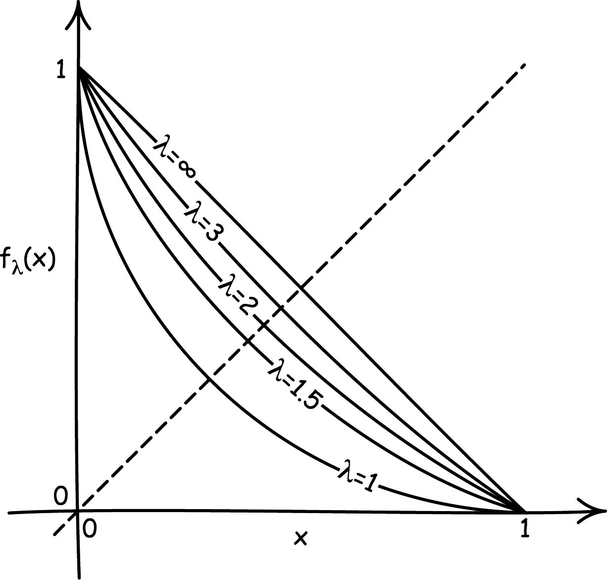
One may imagine that such self-inverting transformations are rare. They are not, and very many can be found. Loosely speaking, they are about as common in the world of functions on reals as are symmetric functions.Footnote ¹⁴ The self-inverting (9a) is the $\lambda =\infty $ member of the λ-indexed family of self-inverting transformationsFootnote ¹⁵

displayed graphically in Figure 1. Another simple member is $\lambda =1$ , which is

That these functions are self-inverting manifests as a symmetry of the graph about the $x^{\prime }=x$ diagonal, represented as a dashed line in Figure 1. Indeed any function with this symmetry property will be self-inverting. It ensures that if $x=a$ is transformed to $x^{\prime }=f_{\lambda }( a) $ , then $x^{\prime }=a$ will also be transformed to the same $x=f_{\lambda }( a) $ by the inverse transformation, as shown in the figure.

Figure 1.

A family of self-inverting transformations.

The probability distribution $p( x) $ must remain invariant under each transformation $f_{\lambda }$ , according to PII, for each yields a perfectly symmetric redescription of the problem. We can see, however, that no $p( x) $ can exhibit this degree of invariance. To see this, we do not need all the properties of the family of self-inverting transformations $f_{\lambda }$ . We need only assume that it has two members, $h_{1}$ and $h_{2}$ , say, such that $h_{1}( x) < h_{2}( x) $ for all $0< x< 1$ . That is trivially achieved using any pair of members of $f_{\lambda }$ , since, for fixed x in $( 0,\, 1) $ , $f_{\lambda }( x) $ is strictly increasing in λ. As before, PII requires that $p( x) $ and its transform $p^{\prime }( x^{\prime }) $ under a self-inverting transformation $x^{\prime }=f_{\lambda }( x) $ must satisfy

Now select any X, such that $0< X< 1$ . For $x^{\prime }_{1}( x) =h_{1}( x) $ , we have from (10a) and (10b) that

Similarly, for $x^{\prime }_{2}( x) =h_{2}( x) $ , we have

Subtracting and relabeling the variable of integration, we have

Since $p( x) \geq 0$ for all x, it follows thatFootnote ¹⁶ $p( x) =0$ for all $x^{\prime }_{1}( X) < x< x^{\prime }_{2}( X) $ . Since X is chosen arbitrarily, we may select X so that any nominated value of x lies in the interval $( x^{\prime }_{1}( X) ,\, x^{\prime }_{2}( X) ) $ .Footnote ¹⁷ Hence it follows that $p( x) =0$ for all $0< x< 1$ , which contradicts the requirement that a probability distribution normalize to unity.

6.1. Invariance under Disjunctive Coarsening and Refinements

We saw in Section 3.1 above that the paradoxes of indifference all depended upon a single idea: if our ignorance is sufficient, we may assign equal beliefs to all members of some partition of the outcome space, and that equality persists through disjunctive coarsenings and refinements. This idea is explored here largely because of its wide acceptance in that literature. I have already indicated above, in Section 3.1, that the idea is less defensible in cases in which there is not a complete symmetry between the two descriptions. We shall see in Sections 6.2 and 6.3 below that the same results about ignorance as derived here in Section 6.1 can be derived from PII using descriptions that are fully symmetric, related by self-inverting transformations.

Let us develop the idea of invariance of ignorance under disjunctive coarsenings and refinements. If we have an outcome space Ω partitioned into mutually contradictory propositions $\Omega =A_{1}\vee A_{2}\vee \cdots \vee A_{n}$ , an example of a disjunctive coarsening is the formation of the new partition of mutually contradictory propositions $\Omega =B_{1}\vee B_{2}\vee \cdots \vee B_{n-1}$ , where

All disjunctive coarsenings of $A_{1},\, A_{2},\,\ldots \, ,\, A_{n}$ are produced by finitely many applications of this coarsening operation along with arbitrary permutations of the propositions, as defined by (1), above. A partition and its coarsening are each nontrivial if none of their propositions is Ω or Φ. The inverse of a coarsening is a refinement.

Assume that we have no grounds for preferring any of the members of the nontrivial partition of $\Omega =A_{1}\vee A_{2}\vee \cdots \vee A_{n}$ . We seek the appropriate degrees of belief $[ A_{i}\vert \Omega ] $ . By PI, we assign equal belief to each, and, by supposition, this ignorance degree of belief $[ \emptyset \vert \Omega ] < I< [ \Omega \vert \Omega ] $ is neither certainty nor complete disbelief:

Now consider the coarsening (12) and assume that we have no grounds for preferring any of the members. Once again there exists a possibly distinct ignorance degree of belief $I^{\prime }$ , neither certainty nor complete disbelief, such that

Since from (12) $B_{1}=A_{1}$ , we have $[ A_{1}\vert \Omega ] =[ B_{1}\vert \Omega ] $ so that $I^{\prime }=I$ . Since all coarsenings are produced by successive applications of (12) along with permutations, it follows that the one ignorance degree of belief I is unique. Finally, if C is a nontrivial disjunction of some proper subset of the $\{ A_{1},\, A_{2},\,\ldots ,\, A_{n}\} $ —written $C=A_{a}\vee \cdots \vee A_{b}$ —some sequence of coarsening and permutations allows us to infer that its degree of confirmation is I. That is, we infer the distinctive property of ignorance presumed in the paradoxes of indifference:Footnote ¹⁸

6.2. Invariance of Ignorance under Negation: The Case of the Code Book

We saw in Section 2.2 above that one application of PII was Jaynes's deduction of the principle of indifference by requiring that a state of ignorance over a finite outcome space remains invariant under a permutation of the propositions. This same idea can also be applied to a transformation that switches propositions with their negations. If we are really ignorant over some outcome A, then our degree of belief in A would be unchanged if A had been somehow switched with its negation, ∼A. A short parable may help clarify the transformation.

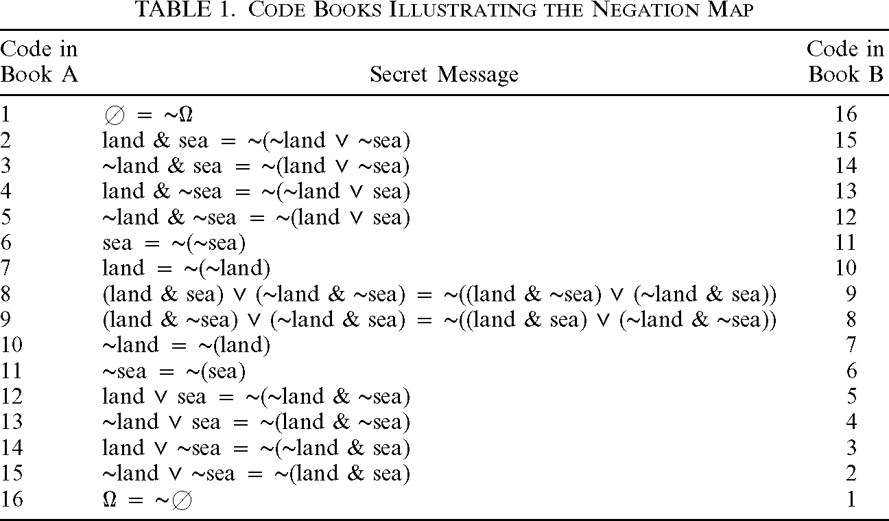
Let us imagine that we are to receive a message pertaining to the two compatible outcomes ‘land’ and ‘sea’ by means of a secret code that assigns numbers to each outcome. The code was devised by a very dedicated logician, so there are numbers for all possible 16 logical combinations of the outcomes. For greater security, we have two code books to choose from. Their values are … (shh—don’t tell! see Table 1).

Table 1.

Code Books Illustrating the Negation Map

Code in Book A	Secret Message	Code in Book B
1	Φ = ∼Ω	16
2	land & sea = ∼(∼land ∨ ∼sea)	15
3	∼land & sea = ∼(land ∨ ∼sea)	14
4	land & ∼sea = ∼(∼land ∨ sea)	13
5	∼land & ∼sea = ∼(land ∨ sea)	12
6	sea = ∼(∼sea)	11
7	land = ∼(∼land)	10
8	(land & sea) ∨ (∼land & ∼sea) = ∼((land & ∼sea) ∨ (∼land & sea))	9
9	(land & ∼sea) ∨ (∼land & sea) = ∼((land & sea) ∨ (∼land & ∼sea))	8
10	∼land = ∼(land)	7
11	∼sea = ∼(sea)	6
12	land ∨ sea = ∼(∼land & ∼sea)	5
13	∼land ∨ sea = ∼(land & ∼sea)	4
14	land ∨ ∼sea = ∼(∼land & sea)	3
15	∼land ∨ ∼sea = ∼(land & sea)	2
16	Ω = ∼Φ	1

Prior to its receipt we are in complete ignorance over which message may come and begin to contemplate how credible the content of each message may be. On the presumption that Book A is in use, we assign beliefs not over which message may come, but over the truth of the 16 possible messages. We must assign maximum belief to the content of code 16, since we know that Ω is necessarily true; we must assign minimum belief to the contents of code 1, since the contradiction Φ is always false; and we assign intermediate, ignorance degrees of belief to everything in between. In convenient symbols,

We now find that it is not Book A, but Book B that will be used. How will that affect our distribution of belief? We must exchange our degrees of belief for the message with codes 1 and 16, since code 1 now designates the necessarily true Ω and code 16 the necessarily false Φ. What of the remaining messages? We had assigned degree of belief $I_{6}$ to what we thought was the message ‘sea’. It now turns out to be the message ‘∼sea’. If our ignorance is sufficient, that will have no effect on our degree of belief. ‘Sea’? ‘∼Sea’? We just do not know! That is, we must assign equal degree of belief to each, so that $I_{6}=I_{11}$ . This analysis can be repeated for all the remaining outcomes 2 to 15. In each case, the switching of the codebooks has simply switched one message with its negation, as the table reveals. For example, under the Book A, code 14 designates ‘land ∨ ∼sea’. Under Book B, code 14 designates its negation ‘∼land & sea’, and the original ‘land ∨ ∼sea’ is designated by code 3. So, by analogous reasoning, $I_{3}=I_{14}$ . We can also infer that all four values are the same by using the property of monotonicity mentioned in Section 5 above.Footnote ¹⁹ Continuing in this way, we can conclude that all intermediate degrees of ignorance have the same value $I=I_{2}=\cdots =I_{15}$ . Rather than displaying the argument in all detail, it is sufficient to proceed to the general case, whose proof covers this special case.

6.3. The General Case

An outcome space, Ω, consists of propositions, $C_{1},\, C_{2},\,\ldots ,\, C_{m}$ , generated by closing a set of atomic propositions $A_{1},\, A_{2},\,\ldots ,\, A_{n}$ , under the usual Boolean operators ∼, ∨, and &, taking note of the usual logical equivalences. The remapping of codebooks corresponds to the negation map, N, between the set of proposition labels $C_{1},\, C_{2},\,\ldots ,\, C_{m}$ and a duplicate set of proposition labels, $C^{\prime }_{1},\, C^{\prime }_{2},\,\ldots ,\, C^{\prime }_{m}$ , in which

What is important about this negation map (15) is that it is self-inverting—the negation of a negation returns the original proposition (or, in this case, its label clone). Thus the sets $C_{i}$ and $C^{\prime }_{i}$ are symmetric descriptionsFootnote ²⁰ and, if we are in ignorance over the outcomes, PII may be applied. The analysis proceeds with the two-component calculation already shown in Section 2.2. Since the map simply relabels the same outcomes, we have

But since we have a perfect symmetry in the two descriptions of the outcomes, we also have, for the contingent propositions (i.e., those that are not always true or always false),Footnote ²¹

It follows immediately from these two conditions (Agreement in Degrees of Belief and Symmetry) that $[ \sim C^{\prime }_{i}\vert \Omega ^{\prime }] =[ C^{\prime }_{i}\vert \Omega ^{\prime }] $ ; or, re-expressed in the original proposition labels,

where this condition holds for every contingent proposition in the outcome space Ω. So far, we cannot preclude that the ignorance degree $I_{i}$ defined is unique for each distinct pair of contingent propositions $C_{i},\,\sim C_{i}$ . As before, monotonicity allows us to infer that all $I_{i}$ are equal to a common value I. To see this, take any two contingent propositions C and D. There are two cases.

We have now used PII to infer that, in cases of ignorance, every contingent proposition in the outcome space Ω must be assigned the same ignorance value I. This is the same result as arrived at in Section 6.1 above by means of the idea that the ignorance state must be invariant under disjunctive coarsenings and refinements. Thus we affirm that both approaches lead us to a unique state of ignorance, in which all contingent propositions are assigned the same ignorance value, I.

There is a more formal way of understanding the generation of this unique ignorance state from the condition of invariance under negation. Elsewhere (Norton Reference Norton2007a), I have investigated how the familiar duality of truth and falsity in a Boolean algebra may be extended to real-valued measures defined on the algebra. To each additive measure, m, there is a dual additive measure, M, defined by the dual map $M( A) =m( \sim A) $ , for each proposition, A, in the algebra. Because additive measures and their duals obey different calculi, additive measures are not self-dual. We arrive at the ignorance state for the case of real valued measures by the simple condition that the measure be self-dual in its contingent propositions.

6.4. Comparing Ignorance across Different Outcome Spaces

The arguments of Sections 6.1, 6.2, and 6.3 establish that, for each outcome space, there exists a unique ignorance degree of belief for all contingent propositions in it. That leaves the possibility that this ignorance degree of belief is different for each distinct outcome space. It is a natural expectation that the same ignorance degree of belief can be found in all outcome spaces. Naturalness, however, is no substitute for demonstration. The difficulty in mounting a demonstration is that the framework sketched in Section 5 is too impoverished to enable comparison of degrees of belief between different outcome spaces. (In a richer system, such comparisons are enabled by Bayes’ theorem or its analog.) Some further assumption is needed to enable the comparison. In this section, I will show that introducing a very weak notion of independence and assuming that it is occasionally instantiated is sufficient to allow us to infer that the same ignorance degree of belief arises in all finite outcome spaces.

Consider an outcome space ‘A’ defined by the logical closure under Boolean operations of m mutually exclusive and exhaustive, contingent propositions $A_{1},\, A_{2},\,\ldots ,\, A_{m}$ , so that $\Omega =A_{1}\vee A_{2}\vee \cdots \vee A_{m}$ . We shall assume that we are in a state of complete ignorance over A so that

for $i=1,\ldots ,\, m$ . The subscript A allows the possibility that the ignorance degree of belief and other degrees of belief are peculiar to the outcome space A. A second outcome space, ‘B’, is defined analogously, with n propositions $B_{1},\, B_{2},\,\ldots ,\, B_{n}$ , for which

where $k=1,\ldots ,\, n$ . Finally, we define a product outcome space, ‘AB’, as generated in the same way by the mn mutually exclusive and exhaustive propositions, $( A_{1}\,\& \, B_{1}) ,\:( A_{1}\,\& \, B_{2}) ,\,\ldots ,\,( A_{m}\,\& \, B_{n}) $ . Degrees of belief relative to this product outcome space are designated by $[ \cdot \vert \Omega ] _{AB}$ .

A very weak notion of independence of the two spaces is

Weak independence of outcome spaces A and B. The degree of belief in every proposition of A is unaffected by the mere knowledge that outcomes in B are possible; and conversely. That is expressed by the condition

for all admissible $i,\, k$ .

This condition is much weaker than the usual condition of probabilistic independence. In the latter, the probability assigned to an outcome of one space is unaffected when the outcome is conditionalized on the supposition that some outcome of the other space obtains. In (17), we conditionalize only on the knowledge that the other outcome space exists, not that one of its outcomes obtains.

An example illustrates the differing strengths. Nothing in the discussion above precludes the propositions $B_{1},\, B_{2},\,\ldots ,\, B_{n}$ of the second outcome space being merely a permutation of the propositions $A_{1},\, A_{2},\,\ldots ,\, A_{m}$ of the first outcome space. In that case, ordinary probabilistic independence between the two spaces would fail. However the weaker sense of (17) would still hold. To see that this weaker sense is not vacuous, imagine a second example in which the propositions of the second outcome space are $B_{1}=A_{1},\, B_{2}=A_{2},\,\ldots ,\, B_{n}=A_{m-1}$ ; that is, the second space allows everything in first but denies $A_{m}$ . (In effect, this is the space generated from the A outcome space by conditioning on $A_{1}\vee \cdots \vee A_{m-1}$ .) Since the B but not the A outcome space presumes that $A_{m}$ is false, we would not expect (17) to hold; for learning the range of possibility admitted by B supplies new information that can alter judgments of degrees of belief. Indeed relation (17) must fail in case $i=m$ , for $[ A_{m}\vert \Omega ] _{A}=I_{A}$ butFootnote ²² $[ A_{m}\vert \Omega ] _{AB}=[ \emptyset \vert \Omega ] _{AB}$ .

If outcome spaces A and B are independent in the sense of (17), then we can show that their ignorance degrees of belief are the same. First note that for this case, we must also have an ignorance distribution in the product space AB, with an ignorance degree $I_{AB}$

for admissible i, k. From the weak notion of independence (17), we also have

Combining, we have

so that the ignorance degree of belief in two independent outcome spaces is the same.

This last conclusion is enough to enable us to conclude the uniqueness of the ignorance degree of belief for all outcome spaces, even ones that are not independent in the sense of (17). To see this, imagine that the outcome spaces A and B are not independent and that their ignorance degrees of belief are I _A and I _B . We need only assume that there exists a third outcome space, C, that is independent from each of A and B in the sense of (17), with ignorance degree of belief I _C . It now follows from (18) that $I_{C}=I_{A}$ and $I_{C}=I_{B}$ . Combining them, we have $I_{A}=I_{B}$ , which establishes the equality of the degrees of ignorance for any two outcome spaces A and B.