2 Available energetics of a stratified compressible binary fluid

We start by revisiting the Andrews (Reference Andrews1981) construction of PE density so as to generalise it easily to multicomponent compressible stratified fluids. As in Andrews (Reference Andrews1981) or Bannon (Reference Bannon2003), we define the PE density of a stratified fluid as the sum of its available elastic energy (AEE) density and APE density. As shown below, this can be achieved without loss of generality by restricting attention to the case of a binary fluid; that is, one whose equation of state for density depends on composition $S$ (referred to as ‘salinity’ hereafter) in addition to specific entropy $\unicode[STIX]{x1D702}$ and pressure $p$ , all quantities being functions of spatial position $(x,y,z)$ and time $t$ . A full set of governing equations in the Earth rotating frame is

(2.1) $$\begin{eqnarray}\displaystyle & \displaystyle \unicode[STIX]{x1D70C}{\displaystyle \frac{\text{D}\boldsymbol{v}}{\text{D}t}}+2\unicode[STIX]{x1D734}\times \unicode[STIX]{x1D70C}\boldsymbol{v}+\unicode[STIX]{x1D735}p=-\unicode[STIX]{x1D70C}\unicode[STIX]{x1D735}\unicode[STIX]{x1D6F7}+\unicode[STIX]{x1D70C}\boldsymbol{F}, & \displaystyle\end{eqnarray}$$

(2.2) $$\begin{eqnarray}\displaystyle & \unicode[STIX]{x1D735}\boldsymbol{\cdot }\boldsymbol{v}={\displaystyle \frac{1}{\unicode[STIX]{x1D710}}}{\displaystyle \frac{\text{D}\unicode[STIX]{x1D710}}{\text{D}t}}, & \displaystyle\end{eqnarray}$$

(2.3) $$\begin{eqnarray}\displaystyle & {\displaystyle \frac{\text{D}(\unicode[STIX]{x1D702},S)}{\text{D}t}}=(\dot{\unicode[STIX]{x1D702}},{\dot{S}}), & \displaystyle\end{eqnarray}$$

(2.4) $$\begin{eqnarray}\displaystyle & \unicode[STIX]{x1D710}=\unicode[STIX]{x1D710}(\unicode[STIX]{x1D702},S,p). & \displaystyle\end{eqnarray}$$

Here, $\boldsymbol{v}=(u,v,w)$ is the velocity field, $\unicode[STIX]{x1D734}$ is the Earth rotation vector, $\unicode[STIX]{x1D6F7}(z)=g_{0}z$ is the geopotential ( $g_{0}$ is gravitational acceleration), $z$ is height, increasing positively upwards, $\unicode[STIX]{x1D710}=1/\unicode[STIX]{x1D70C}$ is the specific volume, $\unicode[STIX]{x1D70C}$ is density, $\boldsymbol{F}$ is frictional force, while $\dot{\unicode[STIX]{x1D702}}$ and ${\dot{S}}$ represent diabatic sources of entropy and salt.

We first address the case of an ideal fluid, thus setting $\boldsymbol{F}=\dot{\unicode[STIX]{x1D702}}={\dot{S}}=0$ in (2.1)–(2.4). In this case, a standard expression for the total energy budget is

(2.5) $$\begin{eqnarray}\displaystyle & \displaystyle \unicode[STIX]{x1D70C}{\displaystyle \frac{\text{D}}{\text{D}t}}\left({\displaystyle \frac{\boldsymbol{v}^{2}}{2}}+\unicode[STIX]{x1D6F7}+e\right)+\unicode[STIX]{x1D735}\boldsymbol{\cdot }(p\boldsymbol{v})=0, & \displaystyle\end{eqnarray}$$

where $e=e(\unicode[STIX]{x1D702},S,p)=h(\unicode[STIX]{x1D702},S,p)-p\unicode[STIX]{x1D710}$ is the specific internal energy and $h$ is the specific enthalpy. In order to obtain an expression for the PE density of the fluid considered, one first needs to identify suitably defined reference specific volume $\unicode[STIX]{x1D710}_{0}(z)$ and pressure $p_{0}(z)$ profiles as functions of $z$ only and in mechanical (hydrostatic) equilibrium,

(2.6) $$\begin{eqnarray}\displaystyle & \displaystyle \unicode[STIX]{x1D710}_{0}(z){\displaystyle \frac{\unicode[STIX]{x2202}p_{0}}{\unicode[STIX]{x2202}z}}(z)=-{\displaystyle \frac{\unicode[STIX]{x2202}\unicode[STIX]{x1D6F7}}{\unicode[STIX]{x2202}z}}(z). & \displaystyle\end{eqnarray}$$

A discussion of the physical issues pertaining to the construction of the reference state is deferred to § 4. The next key step is to assign to each fluid parcel a reference position $z_{r}(\unicode[STIX]{x1D702},S)$ in that reference state. This can be done most generally by regarding $z_{r}$ as the particular depth at which the specific volume of the fluid parcel moved adiabatically to that level matches that of the reference state. Mathematically, this is equivalent to defining $z_{r}$ as a solution of the so-called level of neutral buoyancy (LNB) equation,

(2.7) $$\begin{eqnarray}\displaystyle & \displaystyle \unicode[STIX]{x1D710}(\unicode[STIX]{x1D702},S,p_{r})=\unicode[STIX]{x1D710}_{0}(z_{r}), & \displaystyle\end{eqnarray}$$

similarly to Tailleux (Reference Tailleux2013b ), where $p_{r}(\unicode[STIX]{x1D702},S)=p_{0}(z_{r}(\unicode[STIX]{x1D702},S))$ . Depending on how the reference specific volume $\unicode[STIX]{x1D710}_{0}(z)$ is defined, (2.7) may have no solution, one solution or even multiple solutions. In the former case, $z_{r}$ should be defined at either the top or the bottom of the domain depending on the buoyancy of the fluid parcel in the actual state (Tailleux Reference Tailleux2013b ). The latter case is rarely encountered in the ocean (Saenz et al. Reference Saenz, Tailleux, Butler, Hughes and Oliver2015) but is commonplace in a moist atmosphere (Wong, Tailleux & Gray Reference Wong, Tailleux and Gray2016; Harris & Tailleux Reference Harris and Tailleux2018). How to select the solution in this case is still poorly understood, however.

Following Andrews (Reference Andrews1981), we next use the following identity:

(2.8) $$\begin{eqnarray}\displaystyle & \displaystyle \unicode[STIX]{x1D735}\boldsymbol{\cdot }(p_{0}\boldsymbol{v})=\boldsymbol{v}\boldsymbol{\cdot }\unicode[STIX]{x1D735}p_{0}-{\displaystyle \frac{p_{0}}{\unicode[STIX]{x1D70C}}}{\displaystyle \frac{\text{D}\unicode[STIX]{x1D70C}}{\text{D}t}}=\unicode[STIX]{x1D70C}{\displaystyle \frac{\text{D}}{\text{D}t}}\left({\displaystyle \frac{p_{0}}{\unicode[STIX]{x1D70C}}}\right), & \displaystyle\end{eqnarray}$$

to rewrite the standard energy budget (2.5) in terms of the perturbation pressure $p-p_{0}$ as follows:

(2.9) $$\begin{eqnarray}\displaystyle & \displaystyle \unicode[STIX]{x1D70C}{\displaystyle \frac{\text{D}}{\text{D}t}}\left({\displaystyle \frac{\boldsymbol{v}^{2}}{2}}+{\mathcal{B}}\right)+\unicode[STIX]{x1D735}\boldsymbol{\cdot }[(p-p_{0})\boldsymbol{v}]=0, & \displaystyle\end{eqnarray}$$

where the quantity

(2.10) $$\begin{eqnarray}\displaystyle & \displaystyle {\mathcal{B}}(z,S,\unicode[STIX]{x1D702},p)=\unicode[STIX]{x1D6F7}(z)+e(\unicode[STIX]{x1D702},S,p)+{\displaystyle \frac{p_{0}(z)}{\unicode[STIX]{x1D70C}(\unicode[STIX]{x1D702},S,p)}} & \displaystyle\end{eqnarray}$$

is a hybrid function of thermodynamic coordinates and height, reminiscent of the non-KE part of the classical Bernoulli head. The introduction of ${\mathcal{B}}$ proves determinant, for it turns out that the quantity

(2.11) $$\begin{eqnarray}\unicode[STIX]{x1D6F1}={\mathcal{B}}-{\mathcal{B}}(z_{r},S,\unicode[STIX]{x1D702},p_{r})=\unicode[STIX]{x1D6F7}(z)-\unicode[STIX]{x1D6F7}(z_{r})+e(\unicode[STIX]{x1D702},S,p)-e(\unicode[STIX]{x1D702},S,p_{r})+{\displaystyle \frac{p_{0}(z)}{\unicode[STIX]{x1D70C}}}-{\displaystyle \frac{p_{r}}{\unicode[STIX]{x1D70C}_{r}}},\end{eqnarray}$$

obtained as the difference between ${\mathcal{B}}$ and its value in the reference state, naturally happens to be positive definite and our sought PE density. The quantity $\unicode[STIX]{x1D6F1}+\boldsymbol{v}^{2}/2$ is then the ‘pseudoenergy’ of Shepherd (Reference Shepherd1993), and obeys the following conservation law:

(2.12) $$\begin{eqnarray}\displaystyle & \displaystyle \unicode[STIX]{x1D70C}{\displaystyle \frac{\text{D}}{\text{D}t}}\left({\displaystyle \frac{\boldsymbol{v}^{2}}{2}}+\unicode[STIX]{x1D6F1}\right)+\unicode[STIX]{x1D735}\boldsymbol{\cdot }[(p-p_{0})\boldsymbol{v}]=0. & \displaystyle\end{eqnarray}$$

To prove its positive definite character, it is useful to rewrite $\unicode[STIX]{x1D6F1}$ in terms of the enthalpies $h(\unicode[STIX]{x1D702},S,p)=e(\unicode[STIX]{x1D702},S,p)+p/\unicode[STIX]{x1D70C}$ and $h(\unicode[STIX]{x1D702},S,p_{r})=e(\unicode[STIX]{x1D702},S,p_{r})+p_{r}/\unicode[STIX]{x1D70C}_{r}$ as follows:

(2.13) $$\begin{eqnarray}\displaystyle & \displaystyle \unicode[STIX]{x1D6F1}=\unicode[STIX]{x1D6F7}(z)-\unicode[STIX]{x1D6F7}(z_{r})+h(\unicode[STIX]{x1D702},S,p)-h(\unicode[STIX]{x1D702},S,p_{r})+{\displaystyle \frac{p_{0}(z)-p}{\unicode[STIX]{x1D70C}}}, & \displaystyle\end{eqnarray}$$

as this naturally yields the decomposition $\unicode[STIX]{x1D6F1}=\unicode[STIX]{x1D6F1}_{1}+\unicode[STIX]{x1D6F1}_{2}$ , where

(2.14) $$\begin{eqnarray}\displaystyle & \displaystyle \unicode[STIX]{x1D6F1}_{1}=h(\unicode[STIX]{x1D702},S,p)-h(\unicode[STIX]{x1D702},S,p_{0}(z))+{\displaystyle \frac{p_{0}(z)-p}{\unicode[STIX]{x1D70C}}}, & \displaystyle\end{eqnarray}$$

(2.15) $$\begin{eqnarray}\displaystyle & \displaystyle \unicode[STIX]{x1D6F1}_{2}=\unicode[STIX]{x1D6F7}(z)-\unicode[STIX]{x1D6F7}(z_{r})-h(\unicode[STIX]{x1D702},S,p_{r})+h(\unicode[STIX]{x1D702},S,p_{0}(z)). & \displaystyle\end{eqnarray}$$

The quantity $\unicode[STIX]{x1D6F1}_{1}$ is the so-called AEE density previously derived by Andrews (Reference Andrews1981) and Bannon (Reference Bannon2003), and may be rewritten as follows:

(2.16) $$\begin{eqnarray}\displaystyle & \displaystyle \unicode[STIX]{x1D6F1}_{1}=\int _{p_{0}(z)}^{p}[\unicode[STIX]{x1D710}(\unicode[STIX]{x1D702},S,p^{\prime })-\unicode[STIX]{x1D710}(\unicode[STIX]{x1D702},S,p)]\,\text{d}p^{\prime }=\int _{p_{0}(z)}^{p}\int _{p^{\prime }}^{p}{\displaystyle \frac{1}{\unicode[STIX]{x1D70C}^{2}c_{s}^{2}}}(\unicode[STIX]{x1D702},S,p^{\prime \prime })\,\text{d}p^{\prime \prime }\,\text{d}p^{\prime }, & \displaystyle\end{eqnarray}$$

where the identities $\text{d}h=T\,\text{d}\unicode[STIX]{x1D702}+\unicode[STIX]{x1D707}\,\text{d}S+\unicode[STIX]{x1D710}\,\text{d}p$ and $\unicode[STIX]{x1D710}_{p}=-(\unicode[STIX]{x1D70C}^{2}c_{s}^{2})^{-1}$ have been used. The result $\unicode[STIX]{x1D6F1}_{1}\geqslant 0$ follows from the $\unicode[STIX]{x1D70C}$ and $c_{s}$ both being strictly positive quantities. For small pressure perturbation $p^{\prime }=p-p_{0}$ , $\unicode[STIX]{x1D6F1}_{1}$ reduces to the well-known quadratic approximation,

(2.17) $$\begin{eqnarray}\displaystyle & \displaystyle \unicode[STIX]{x1D6F1}_{1}\approx {\displaystyle \frac{(p-p_{0}(z))^{2}}{2\unicode[STIX]{x1D70C}^{2}c_{s}^{2}}}, & \displaystyle\end{eqnarray}$$

as noted by Andrews (Reference Andrews1981) and Shepherd (Reference Shepherd1993), among others. Physically, $\unicode[STIX]{x1D6F1}_{1}$ represents the work required to bring the reference pressure $p_{0}(z)$ of a fluid parcel to its actual pressure $p$ by means of an adiabatic compression $(p>p_{0})$ or expansion $(p<p_{0})$ . Andrews (Reference Andrews1981) argues that such a term vanishes in the incompressible limit $c_{s}\rightarrow +\infty$ , thus justifying its absence in Boussinesq fluids.

The quantity $\unicode[STIX]{x1D6F1}_{2}$ is the APE density of the fluid and is the only part of the PE density generally retained in incompressible Boussinesq fluids. Physically, it is equivalent to the $\unicode[STIX]{x1D6F1}_{2}$ of Andrews (Reference Andrews1981), but, mathematically, (2.15) is actually much simpler. Moreover, in contrast to the constructions of Andrews (Reference Andrews1981) and Bannon (Reference Bannon2003), it does not require the introduction of purely depth-dependent reference profiles for specific entropy and salinity, which is overly restrictive in real fluids. In order to clarify the link between the APE density of a compressible fluid and that of the Boussinesq or hydrostatic primitive equations, we make use of (2.6) and the change of variables $p^{\prime }=p_{0}(z^{\prime })$ , $\text{d}p^{\prime }=-\unicode[STIX]{x1D70C}_{0}(z^{\prime })g_{0}\,\text{d}z^{\prime }$ to rewrite $\unicode[STIX]{x1D6F1}_{2}$ in the following mathematically equivalent ways:

(2.18) $$\begin{eqnarray}\displaystyle \displaystyle \unicode[STIX]{x1D6F1}_{2} & = & \displaystyle -\int _{z_{r}}^{z}\unicode[STIX]{x1D710}_{0}(z^{\prime }){\displaystyle \frac{\text{d}p_{0}}{\text{d}z}}(z^{\prime })\,\text{d}z^{\prime }+\int _{p_{0}(z_{r})}^{p_{0}(z)}\unicode[STIX]{x1D710}(\unicode[STIX]{x1D702},S,p^{\prime })\,\text{d}p^{\prime }\nonumber\\ \displaystyle \displaystyle & = & \displaystyle \int _{p_{0}(z_{r})}^{p_{0}(z)}[\unicode[STIX]{x1D710}(\unicode[STIX]{x1D702},S,p^{\prime })-\hat{\unicode[STIX]{x1D710}}_{0}(p^{\prime })]\,\text{d}p^{\prime }=g_{0}\int _{z_{r}}^{z}{\displaystyle \frac{[\unicode[STIX]{x1D70C}(\unicode[STIX]{x1D702},S,p_{0}(z^{\prime }))-\unicode[STIX]{x1D70C}_{0}(z^{\prime })]}{\unicode[STIX]{x1D70C}(\unicode[STIX]{x1D702},S,p_{0}(z^{\prime }))}}\,\text{d}z^{\prime },\quad\end{eqnarray}$$

where $\hat{\unicode[STIX]{x1D710}}_{0}(p)=\unicode[STIX]{x1D710}_{0}(Z_{0}(p))$ , $Z_{0}(p)$ being the inverse function of $p_{0}(z)$ satisfying $p_{0}(Z_{0}(p))=p$ . Equations (2.18) are classical expressions for the work against buoyancy forces required to move a fluid parcel from its reference position at pressure $p_{r}=p_{0}(z_{r})$ to its actual position at pressure $p_{0}(z)$ by means of an adiabatic and isohaline process. It is easily seen that the APE density for a Boussinesq fluid derived by Holliday & McIntyre (Reference Holliday and McIntyre1981) or Tailleux (Reference Tailleux2013c ) can be recovered (1) by replacing the denominator $\unicode[STIX]{x1D70C}(\unicode[STIX]{x1D702},S,p)$ in the last term of (2.18) by the constant reference Boussinesq density $\unicode[STIX]{x1D70C}_{00}$ and (2) by replacing everywhere the reference pressure $p_{0}(z)$ by the Boussinesq pressure $p_{00}(z)=-\unicode[STIX]{x1D70C}_{00}g_{0}z$ . As to the APE density for a hydrostatic dry atmosphere discussed by Novak & Tailleux (Reference Novak and Tailleux2018), it is simply recovered from the first term in (2.18) by replacing the upper bound $p_{0}$ by the hydrostatic pressure $p$ itself. As a result, the arguments of Tailleux (Reference Tailleux2013b ) may be used to prove the positive definite character of $\unicode[STIX]{x1D6F1}$ , as well as its small-amplitude approximation $\unicode[STIX]{x1D6F1}_{2}\approx N_{r}^{2}(z-z_{r})^{2}/2$ , with $N_{r}^{2}$ given by

(2.19) $$\begin{eqnarray}\displaystyle & \displaystyle N_{r}^{2}=-{\displaystyle \frac{g_{0}}{\unicode[STIX]{x1D70C}_{r}}}\left[{\displaystyle \frac{\text{d}\unicode[STIX]{x1D70C}_{0}}{\text{d}z}}(z_{r})+{\displaystyle \frac{\unicode[STIX]{x1D70C}_{r}g_{0}}{c_{s}^{2}(S,\unicode[STIX]{x1D702},p_{r})}}\right]. & \displaystyle\end{eqnarray}$$

It should be noted here that in a binary or multicomponent fluid, the possibility of density compensation means that only the reference density and pressure profiles may be assumed to be functions of $z$ alone; all other quantities, including $N_{r}^{2}$ , must in general depend on horizontal position as well. To conclude, let us remark that $\unicode[STIX]{x1D6F1}$ is ‘local’ only in the sense of being definable at any location, since it possesses some degree of non-locality due to being defined relative to a ‘globally defined’ reference state. For this reason, $\unicode[STIX]{x1D6F1}$ is best viewed as a sophisticated form of density variance, which – like other standard statistical quantities such as ‘anomalies’ – is also non-local in some sense.

3 Energy conversions in the presence of diabatic sinks and sources

We now turn to the issue of how diabatic sinks and sources of $(\unicode[STIX]{x1D702},S)$ affect the evolution of the PE density. To that end, we reintroduce the diabatic terms $(\dot{\unicode[STIX]{x1D702}},{\dot{S}})$ in the equations for $(\unicode[STIX]{x1D702},S)$ . Because the reference state may be altered by diabatic effects, we assume from now on that the specific volume and pressure reference profiles $\unicode[STIX]{x1D710}_{0}(z,t)$ and $p_{0}(z,t)$ also depend on time (Winters et al. Reference Winters, Lombard, Riley and d’Asaro1995). The LNB equation (2.7) thus becomes $\unicode[STIX]{x1D710}[\unicode[STIX]{x1D702},S,p_{0}(z_{r},t)]=\unicode[STIX]{x1D710}_{0}(z_{r},t)$ and now defines $z_{r}=z_{r}(\unicode[STIX]{x1D702},S,t)$ as a time-dependent material function of $(\unicode[STIX]{x1D702},S)$ . Evolution equations for $\unicode[STIX]{x1D6F1}_{1}$ and $\unicode[STIX]{x1D6F1}_{2}$ are obtained by taking the material derivatives of (2.14) and (2.15). The addition of an evolution equation for the KE $E_{k}=\boldsymbol{v}^{2}/2$ (obtained in the usual way) yields the following description of energetics:

(3.1) $$\begin{eqnarray}\displaystyle & \displaystyle \unicode[STIX]{x1D70C}{\displaystyle \frac{\text{D}E_{k}}{\text{D}t}}+\unicode[STIX]{x1D735}\boldsymbol{\cdot }[(p-p_{0})\boldsymbol{v}]=-\unicode[STIX]{x1D735}\boldsymbol{\cdot }(p_{0}\boldsymbol{v})+{\displaystyle \frac{p}{\unicode[STIX]{x1D710}}}{\displaystyle \frac{\text{D}\unicode[STIX]{x1D710}}{\text{D}t}}-\unicode[STIX]{x1D70C}{\displaystyle \frac{\text{D}\unicode[STIX]{x1D6F7}}{\text{D}t}}+\unicode[STIX]{x1D70C}\boldsymbol{F}\boldsymbol{\cdot }\boldsymbol{v}, & \displaystyle\end{eqnarray}$$

(3.2) $$\begin{eqnarray}\displaystyle & \displaystyle \unicode[STIX]{x1D70C}{\displaystyle \frac{\text{D}\unicode[STIX]{x1D6F1}_{1}}{\text{D}t}}=\unicode[STIX]{x1D735}\boldsymbol{\cdot }(p_{0}\boldsymbol{v})-{\displaystyle \frac{p}{\unicode[STIX]{x1D710}}}{\displaystyle \frac{\text{D}\unicode[STIX]{x1D710}}{\text{D}t}}+\unicode[STIX]{x1D70C}\dot{\unicode[STIX]{x1D6F1}}_{1}+\left(1-{\displaystyle \frac{\unicode[STIX]{x1D70C}}{\unicode[STIX]{x1D70C}_{h}}}\right){\displaystyle \frac{\unicode[STIX]{x2202}p_{0}}{\unicode[STIX]{x2202}t}}(z,t)+{\displaystyle \frac{\unicode[STIX]{x1D70C}_{0}}{\unicode[STIX]{x1D70C}_{h}}}\unicode[STIX]{x1D70C}{\displaystyle \frac{\text{D}\unicode[STIX]{x1D6F7}}{\text{D}t}}, & \displaystyle\end{eqnarray}$$

(3.3) $$\begin{eqnarray}\displaystyle & \displaystyle \unicode[STIX]{x1D70C}{\displaystyle \frac{\text{D}\unicode[STIX]{x1D6F1}_{2}}{\text{D}t}}=\unicode[STIX]{x1D70C}{\displaystyle \frac{\text{D}\unicode[STIX]{x1D6F7}}{\text{D}t}}+\unicode[STIX]{x1D70C}\dot{\unicode[STIX]{x1D6F1}}_{2}-{\displaystyle \frac{\unicode[STIX]{x1D70C}_{0}}{\unicode[STIX]{x1D70C}_{h}}}\unicode[STIX]{x1D70C}{\displaystyle \frac{\text{D}\unicode[STIX]{x1D6F7}}{\text{D}t}}+{\displaystyle \frac{\unicode[STIX]{x1D70C}}{\unicode[STIX]{x1D70C}_{h}}}{\displaystyle \frac{\unicode[STIX]{x2202}p_{0}}{\unicode[STIX]{x2202}t}}(z,t)-{\displaystyle \frac{\unicode[STIX]{x1D70C}}{\unicode[STIX]{x1D70C}_{r}}}{\displaystyle \frac{\unicode[STIX]{x2202}p_{0}}{\unicode[STIX]{x2202}t}}(z_{r},t). & \displaystyle\end{eqnarray}$$

In (3.2) and (3.3), the local diabatic production terms $\dot{\unicode[STIX]{x1D6F1}}_{1}$ and $\dot{\unicode[STIX]{x1D6F1}}_{2}$ are defined by

(3.4a,b ) $$\begin{eqnarray}\displaystyle & \displaystyle \dot{\unicode[STIX]{x1D6F1}}_{1}=(T-T_{h})\dot{\unicode[STIX]{x1D702}}+(\unicode[STIX]{x1D707}-\unicode[STIX]{x1D707}_{h}){\dot{S}},\quad \dot{\unicode[STIX]{x1D6F1}}_{2}=(T_{h}-T_{r})\dot{\unicode[STIX]{x1D702}}+(\unicode[STIX]{x1D707}_{h}-\unicode[STIX]{x1D707}_{r}){\dot{S}}, & \displaystyle\end{eqnarray}$$

where $T$ and $\unicode[STIX]{x1D707}$ denote in situ temperature and relative chemical potential respectively. Moreover, the suffix ‘ $h$ ’ indicates a variable estimated at the pressure $p_{0}(z,t)$ , e.g. $T_{h}=T(\unicode[STIX]{x1D702},S,p_{0}(z,t))$ , while the suffix ‘ $r$ ’ indicates a variable estimated at the pressure $p_{r}=p_{0}(z_{r},t)$ , e.g. $T_{r}=T(\unicode[STIX]{x1D702},S,p_{r})=T(\unicode[STIX]{x1D702},S,p_{0}(z_{r},t))$ . Addition of (3.2) and (3.3) yields the following equation for $\unicode[STIX]{x1D6F1}$ :

(3.5) $$\begin{eqnarray}\displaystyle & \displaystyle \unicode[STIX]{x1D70C}{\displaystyle \frac{\text{D}\unicode[STIX]{x1D6F1}}{\text{D}t}}=\underbrace{\unicode[STIX]{x1D735}\boldsymbol{\cdot }(p_{0}\boldsymbol{v})+\unicode[STIX]{x1D70C}{\displaystyle \frac{\text{D}\unicode[STIX]{x1D6F7}}{\text{D}t}}-{\displaystyle \frac{p}{\unicode[STIX]{x1D710}}}{\displaystyle \frac{\text{D}\unicode[STIX]{x1D710}}{\text{D}t}}}_{C(E_{k},\unicode[STIX]{x1D6F1})}+\unicode[STIX]{x1D70C}\dot{\unicode[STIX]{x1D6F1}}+{\displaystyle \frac{\unicode[STIX]{x2202}p_{0}}{\unicode[STIX]{x2202}t}}(z,t)-{\displaystyle \frac{\unicode[STIX]{x1D70C}}{\unicode[STIX]{x1D70C}_{r}}}{\displaystyle \frac{\unicode[STIX]{x2202}p_{0}}{\unicode[STIX]{x2202}t}}(z_{r},t), & \displaystyle\end{eqnarray}$$

where the local diabatic production/destruction term $\dot{\unicode[STIX]{x1D6F1}}$ is defined by

(3.6) $$\begin{eqnarray}\displaystyle & \displaystyle \dot{\unicode[STIX]{x1D6F1}}=(T-T_{r})\dot{\unicode[STIX]{x1D702}}+(\unicode[STIX]{x1D707}-\unicode[STIX]{x1D707}_{r}){\dot{S}}. & \displaystyle\end{eqnarray}$$

It should be noted that because the diabatic terms ${\dot{S}}$ and $\dot{\unicode[STIX]{x1D702}}$ couple $\unicode[STIX]{x1D6F1}$ to the background potential energy ${\mathcal{B}}_{r}=\unicode[STIX]{x1D6F7}(z_{r})+e(\unicode[STIX]{x1D702},S,p_{r})+p_{r}/\unicode[STIX]{x1D70C}_{r}$ , the pseudoenergy $E_{k}+\unicode[STIX]{x1D6F1}$ is no longer a conservative quantity.

Table 1.

The two different possible approaches to defining the energy conversions between $E_{k}$ , $\unicode[STIX]{x1D6F1}_{1}$ and $\unicode[STIX]{x1D6F1}_{2}$ in a turbulent multicomponent compressible stratified fluid discussed in this paper.

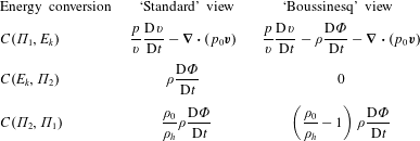
We now discuss the nature of the energy conversions between $E_{k}$ , $\unicode[STIX]{x1D6F1}_{1}$ and $\unicode[STIX]{x1D6F1}_{2}$ implied by (3.1)–(3.3) in order to understand their links with Boussinesq energetics. As is well known, such an exercise is prone to conceptual difficulties, because there is no universally agreed way to define energy conversions, which can often be defined in several plausible mathematically equivalent ways. In the present case, for instance, there appear to be two natural such ways – synthesised in table 1 – which we refer to as the ‘standard’ and ‘Boussinesq’ conversions. The standard conversions are those that naturally follow from the energy budget written as (3.1)–(3.3), and consist of regarding the work of compression/expansion as a conversion between KE and AEE and the term $\unicode[STIX]{x1D70C}g_{0}w$ as a conversion between KE and APE. In this standard view, ‘large’ conversions are permitted to occur between all of the different energy reservoirs. The Boussinesq view, on the other hand, exploits the tendency for the standard energy conversions to compensate each other, thus suggesting that the terms of (3.2) and (3.3) should be recombined as follows:

(3.7) $$\begin{eqnarray}\displaystyle & \displaystyle \unicode[STIX]{x1D70C}{\displaystyle \frac{\text{D}\unicode[STIX]{x1D6F1}_{1}}{\text{D}t}}=\underbrace{\unicode[STIX]{x1D735}\boldsymbol{\cdot }(p_{0}\boldsymbol{v})+\unicode[STIX]{x1D70C}{\displaystyle \frac{\text{D}\unicode[STIX]{x1D6F7}}{\text{D}t}}-{\displaystyle \frac{p}{\unicode[STIX]{x1D710}}}{\displaystyle \frac{\text{D}\unicode[STIX]{x1D710}}{\text{D}t}}}_{C(E_{k},\unicode[STIX]{x1D6F1}_{1})}+\unicode[STIX]{x1D70C}\dot{\unicode[STIX]{x1D6F1}}_{1}-\underbrace{\left(1-{\displaystyle \frac{\unicode[STIX]{x1D70C}_{0}}{\unicode[STIX]{x1D70C}_{h}}}\right)\unicode[STIX]{x1D70C}{\displaystyle \frac{\text{D}\unicode[STIX]{x1D6F7}}{\text{D}t}}}_{C(\unicode[STIX]{x1D6F1}_{1},\unicode[STIX]{x1D6F1}_{2})}+\,\text{N.L.}, & \displaystyle\end{eqnarray}$$

(3.8) $$\begin{eqnarray}\displaystyle & \displaystyle \unicode[STIX]{x1D70C}{\displaystyle \frac{\text{D}\unicode[STIX]{x1D6F1}_{2}}{\text{D}t}}=\underbrace{\left(1-{\displaystyle \frac{\unicode[STIX]{x1D70C}_{0}}{\unicode[STIX]{x1D70C}_{h}}}\right)\unicode[STIX]{x1D70C}{\displaystyle \frac{\text{D}\unicode[STIX]{x1D6F7}}{\text{D}t}}}_{C(\unicode[STIX]{x1D6F1}_{1},\unicode[STIX]{x1D6F1}_{2})}+\unicode[STIX]{x1D70C}\dot{\unicode[STIX]{x1D6F1}}_{2}+\,\text{ N.L.}, & \displaystyle\end{eqnarray}$$

where the acronym N.L. denotes the non-local terms proportional to the various $\unicode[STIX]{x2202}p_{0}/\unicode[STIX]{x2202}t$ partial derivatives. The Boussinesq reorganisation has the key advantage of transforming $C(\unicode[STIX]{x1D6F1}_{1},\unicode[STIX]{x1D6F1}_{2})$ into a density flux anomaly, without actually introducing any form of average. This makes it arguably more relevant/useful to the study of turbulent stratified fluids than the standard view. Physically, (3.7)–(3.8) no longer allow for any direct conversion between KE and the APE density $\unicode[STIX]{x1D6F1}_{2}$ , so that conversion between KE and $\unicode[STIX]{x1D6F1}_{2}$ appears to be indirect and mediated via $\unicode[STIX]{x1D6F1}_{1}$ . As one referee put it, $\unicode[STIX]{x1D6F1}_{1}$ becomes a ‘pass-through’ energy reservoir. The usefulness of this property becomes evident in the incompressible limit $c_{s}\rightarrow +\infty$ . Indeed, in this case, $\unicode[STIX]{x1D6F1}_{1}$ vanishes but the energy conversions on the right-hand side of (3.7) do not. As a consequence, (3.7) becomes a diagnostic equation imposing that the following balance holds approximately at all times:

(3.9) $$\begin{eqnarray}\displaystyle & \displaystyle \underbrace{\unicode[STIX]{x1D735}\boldsymbol{\cdot }(p_{0}\boldsymbol{v})+\unicode[STIX]{x1D70C}{\displaystyle \frac{\text{D}\unicode[STIX]{x1D6F7}}{\text{D}t}}-{\displaystyle \frac{p}{\unicode[STIX]{x1D710}}}{\displaystyle \frac{\text{D}\unicode[STIX]{x1D710}}{\text{D}t}}}_{C(E_{k},\unicode[STIX]{x1D6F1}_{1})}+\unicode[STIX]{x1D70C}\dot{\unicode[STIX]{x1D6F1}}_{1}-\underbrace{\left(1-{\displaystyle \frac{\unicode[STIX]{x1D70C}_{0}}{\unicode[STIX]{x1D70C}_{h}}}\right)\unicode[STIX]{x1D70C}{\displaystyle \frac{\text{D}\unicode[STIX]{x1D6F7}}{\text{D}t}}}_{C(\unicode[STIX]{x1D6F1}_{1},\unicode[STIX]{x1D6F1}_{2})}+\,\text{ N.L.}\approx 0. & \displaystyle\end{eqnarray}$$

If $\unicode[STIX]{x1D70C}\dot{\unicode[STIX]{x1D6F1}}_{1}$ and N.L. can be neglected in (3.9), the above balance reduces to $C(\unicode[STIX]{x1D6F1}_{1},\unicode[STIX]{x1D6F1}_{2})\approx C(E_{k},\unicode[STIX]{x1D6F1}_{1})$ , which formally allows one to regard the density flux anomaly $C(\unicode[STIX]{x1D6F1}_{1},\unicode[STIX]{x1D6F1}_{2})$ as a conversion between KE and $\unicode[STIX]{x1D6F1}_{2}$ , precisely as in Boussinesq energetics. Any KE converted into $\unicode[STIX]{x1D6F1}_{1}$ is instantaneously converted into $\unicode[STIX]{x1D6F1}_{2}$ , and conversely. To establish that such a view is valid and physically meaningful, one presumably would need to prove that such conversions are primarily achieved by sound waves, as these are the only ones capable of transmitting information at infinite speed in the limit $c_{s}\rightarrow +\infty$ , but this is a challenging technical issue that we regard as being beyond the scope of this paper.

4 Issues pertaining to the choice of reference state

How to define and construct the APE reference state has been a continuing source of confusion and difficulty in APE theory since its inception. To date, the issue remains controversial and outstanding. Here, we briefly review and discuss two well-known key difficulties in §§ 4.1 and 4.2 below. The first one pertains to the possible use of ‘non-resting’ reference states. The second one pertains to the apparent arbitrariness of the reference state in local APE theory and whether it implies the possibility of using reference states other than those originally proposed by Lorenz (Reference Lorenz1955).

4.1 Resting versus non-resting reference states

The standard form of APE is commonly understood to originate from horizontal variations in the density field, and therefore is naturally defined relative to a ‘resting’ reference state function of $z$ only (aside from possible temporal dependence). A common objection, however, is that in the presence of rotation, idealised fluid flow configurations such as steady and stable zonal flows or vortices may have a large fraction of their APE actually locked up by a geostrophic or higher-order type of balance and therefore seemingly unavailable. Such examples have prompted a few authors to look for a generalisation of APE to account for momentum constraints, e.g. Codoban & Shepherd (Reference Codoban and Shepherd2003), Andrews (Reference Andrews2006). Whether such an approach is necessarily the ‘right’ one is not clear, however. Indeed, the alternative and much simpler approach advocated here considers that the definition of APE should not depend on the presence of rotation and flow stability, and that the potential energy density $\unicode[STIX]{x1D6F1}_{e}$ defined relative to a non-resting reference state should be regarded as a form of ‘eddy’ potential energy in a mean/eddy decomposition $\unicode[STIX]{x1D6F1}=\unicode[STIX]{x1D6F1}_{e}+\unicode[STIX]{x1D6F1}_{m}+\unicode[STIX]{x1D6FF}\unicode[STIX]{x1D6F1}$ of the total potential energy density $\unicode[STIX]{x1D6F1}$ . Such an approach is easily implemented in the present framework by noting that the construction of $\unicode[STIX]{x1D6F1}$ outlined in § 2 applies equally well to reference pressure and specific volume $p_{m}(x,y,z)$ and $\unicode[STIX]{x1D710}_{m}(x,y,z)$ that also depend on horizontal position. As a result, the above components of the partition of $\unicode[STIX]{x1D6F1}$ can be explicitly defined by

(4.1) $$\begin{eqnarray}\displaystyle & \displaystyle \unicode[STIX]{x1D6F1}_{e}=\unicode[STIX]{x1D6F7}(z)-\unicode[STIX]{x1D6F7}(z_{rm})+e(\unicode[STIX]{x1D702},S,p)-e(\unicode[STIX]{x1D702},S,p_{rm})+{\displaystyle \frac{p_{m}(x,y,z)}{\unicode[STIX]{x1D70C}}}-{\displaystyle \frac{p_{rm}}{\unicode[STIX]{x1D70C}_{rm}}}, & \displaystyle\end{eqnarray}$$

(4.2) $$\begin{eqnarray}\displaystyle & \displaystyle \unicode[STIX]{x1D6F1}_{m}=\unicode[STIX]{x1D6F7}(z_{rm})-\unicode[STIX]{x1D6F7}(z_{r})+e(\unicode[STIX]{x1D702},S,p_{rm})-e(\unicode[STIX]{x1D702},S,p_{r})+{\displaystyle \frac{p_{0}(z_{rm})}{\unicode[STIX]{x1D70C}_{rm}}}-{\displaystyle \frac{p_{r}}{\unicode[STIX]{x1D70C}_{r}}}, & \displaystyle\end{eqnarray}$$

(4.3) $$\begin{eqnarray}\displaystyle & \displaystyle \unicode[STIX]{x1D6FF}\unicode[STIX]{x1D6F1}={\displaystyle \frac{p_{0}(z)-p_{m}(x,y,z)}{\unicode[STIX]{x1D70C}}}+{\displaystyle \frac{p_{m}(x,y,z_{rm})-p_{0}(z_{rm})}{\unicode[STIX]{x1D70C}_{rm}}}. & \displaystyle\end{eqnarray}$$

In (4.1)–(4.3), $p_{r}=p_{r}(\unicode[STIX]{x1D702},S)$ , $\unicode[STIX]{x1D70C}_{r}=\unicode[STIX]{x1D70C}_{r}(\unicode[STIX]{x1D702},S)$ and $z_{r}=z_{r}(\unicode[STIX]{x1D702},S)$ have the same meanings as in § 2 and are functions of the materially conserved variables $(\unicode[STIX]{x1D702},S)$ only, whereas $z_{rm}$ is the reference depth solution of the LNB equation for the non-resting state $\unicode[STIX]{x1D710}(\unicode[STIX]{x1D702},S,p(x,y,z_{rm}))=\unicode[STIX]{x1D710}_{m}(x,y,z_{rm})$ , with $p_{rm}=p_{m}(x,y,z_{rm})$ . Physically, $\unicode[STIX]{x1D6F1}_{e}$ represents the ‘eddy’ potential energy density of a fluid parcel relative to the ‘non-resting’ mean state, whereas $\unicode[STIX]{x1D6F1}_{m}$ represents the potential energy density of the fluid parcel in its mean equilibrium position relative to its ‘resting’ equilibrium position. It should be noted that the above mean/eddy partition of $\unicode[STIX]{x1D6F1}$ does not explicitly depend on the introduction of any particular averaging operator, and is valid for arbitrarily defined ‘non-resting’ and ‘resting’ reference states $(p_{m},\unicode[STIX]{x1D710}_{m})$ and $(p_{0},\unicode[STIX]{x1D710}_{0})$ ; from a mathematical viewpoint, it is the counterpart of the mean/eddy partitioning of the KE as $\boldsymbol{v}^{2}/2=\boldsymbol{v}_{m}^{2}/2+\boldsymbol{v}_{e}^{2}/2+\boldsymbol{v}_{m}\boldsymbol{\cdot }\boldsymbol{v}_{e}$ , which also does not require the introduction of any particular averaging operator. The interaction term $\unicode[STIX]{x1D6FF}\unicode[STIX]{x1D6F1}$ can a priori takes on both signs, and is the counterpart of the interaction $\boldsymbol{v}_{m}\boldsymbol{\cdot }\boldsymbol{v}_{e}$ .

Physically, the expectation is that if $(p_{m},\unicode[STIX]{x1D710}_{m})$ correspond to a steady and stable zonal flow or vortex, rotation should inhibit conversions between $\unicode[STIX]{x1D6F1}_{m}$ and $\unicode[STIX]{x1D6F1}_{e}$ . To confirm this, let use derive the evolution equations for $\boldsymbol{v}^{2}/2+\unicode[STIX]{x1D6F1}_{e}$ , $\unicode[STIX]{x1D6F1}_{m}$ and $\unicode[STIX]{x1D6FF}\unicode[STIX]{x1D6F1}$ in the usual manner,

(4.4) $$\begin{eqnarray}\displaystyle & \displaystyle \unicode[STIX]{x1D70C}{\displaystyle \frac{\text{D}}{\text{D}t}}\left({\displaystyle \frac{\boldsymbol{v}^{2}}{2}}+\unicode[STIX]{x1D6F1}_{e}\right)+\unicode[STIX]{x1D735}\boldsymbol{\cdot }\{[p-p_{m}(x,y,z)]\boldsymbol{v}\}=-{\displaystyle \frac{\unicode[STIX]{x1D70C}\boldsymbol{u}\boldsymbol{\cdot }\unicode[STIX]{x1D735}_{h}p_{rm}}{\unicode[STIX]{x1D70C}_{rm}}}, & \displaystyle\end{eqnarray}$$

(4.5) $$\begin{eqnarray}\displaystyle & \displaystyle \unicode[STIX]{x1D70C}{\displaystyle \frac{\text{D}\unicode[STIX]{x1D6F1}_{m}}{\text{D}t}}+\unicode[STIX]{x1D735}\boldsymbol{\cdot }\left\{{\displaystyle \frac{\unicode[STIX]{x1D70C}[p_{rm}-p_{0}(z_{rm})]\boldsymbol{v}}{\unicode[STIX]{x1D70C}_{rm}}}\right\}={\displaystyle \frac{\unicode[STIX]{x1D70C}\boldsymbol{u}\boldsymbol{\cdot }\unicode[STIX]{x1D735}_{h}p_{rm}}{\unicode[STIX]{x1D70C}_{rm}}}, & \displaystyle\end{eqnarray}$$

(4.6) $$\begin{eqnarray}\displaystyle & \displaystyle \unicode[STIX]{x1D70C}{\displaystyle \frac{\text{D}(\unicode[STIX]{x1D6FF}\unicode[STIX]{x1D6F1})}{\text{D}t}}=\unicode[STIX]{x1D735}\boldsymbol{\cdot }\left\{\left[p_{0}(z)-p_{m}(x,y,z)+{\displaystyle \frac{\unicode[STIX]{x1D70C}(p_{rm}-p_{0}(z_{rm}))}{\unicode[STIX]{x1D70C}_{rm}}}\right]\boldsymbol{v}\right\}, & \displaystyle\end{eqnarray}$$

where $\unicode[STIX]{x1D735}_{h}$ denotes the horizontal part of the gradient operator. It is easily verified that by summing (4.4)–(4.6), one recovers (2.5). Equations (4.4)–(4.5) show that the conversion between $\unicode[STIX]{x1D6F1}_{m}$ and $\unicode[STIX]{x1D6F1}_{e}$ is controlled by the product of the horizontal velocity times the horizontal gradient of $p_{rm}$ , which vanishes for a steady geostrophically balanced state $\boldsymbol{u}\propto f_{0}^{-1}\boldsymbol{k}\times \unicode[STIX]{x1D735}_{h}p_{rm}$ , where $f_{0}$ denotes the local rotation rate and $\boldsymbol{k}$ the unit vector pointing upwards. Therefore, as far as we can judge, the inhibiting effects of rotation can be understood in the context of the mean/eddy decomposition of $\unicode[STIX]{x1D6F1}$ (see Scotti & White (Reference Scotti and White2014) and Novak & Tailleux (Reference Novak and Tailleux2018) for alternative ways of performing such a decomposition), and do not therefore seem to require a definition of APE accounting for momentum constraints. Obviously, this is a subtle and complicated issue that will warrant extensive discussion in a separate and forthcoming dedicated paper.