1 Introduction
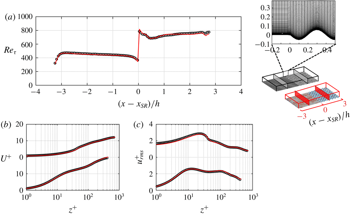
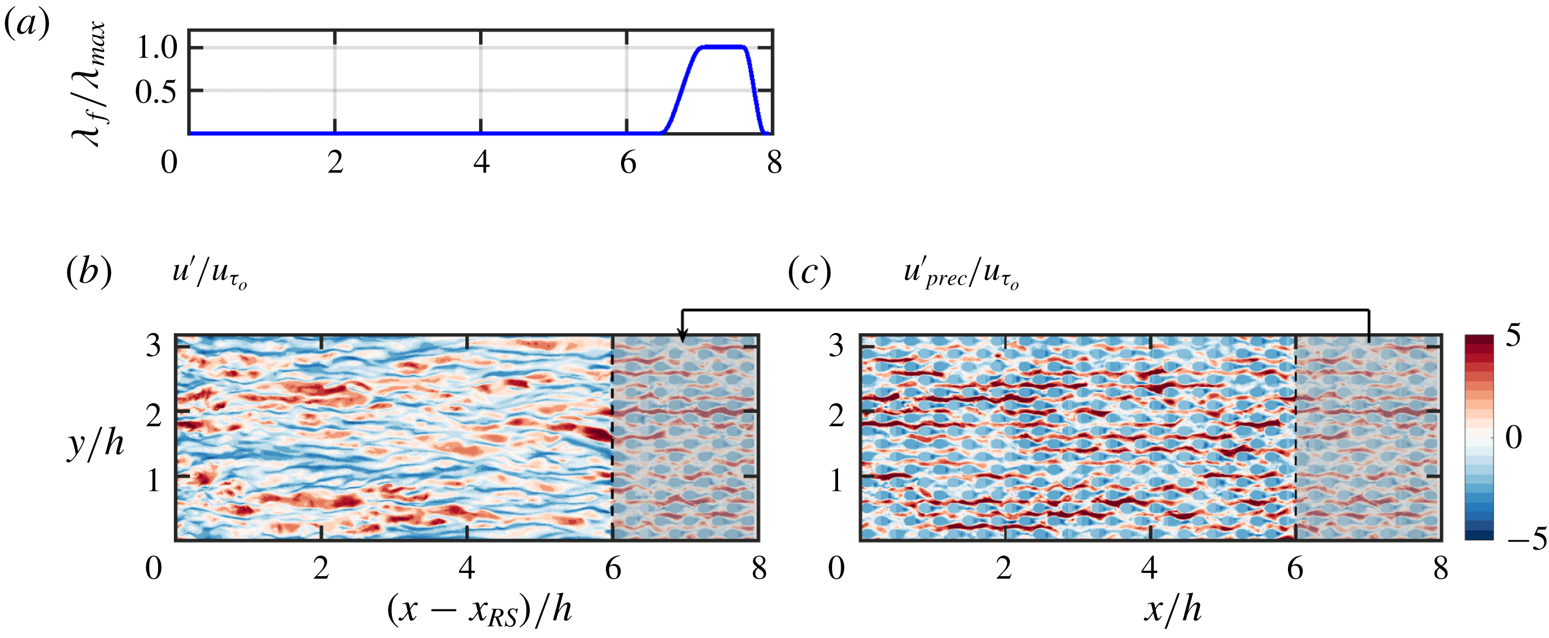
Changes in surface roughness occur in many fabricated or natural applications. Examples include the edges of forests, wind farms or the bio-fouled patches on a ship hull. Surface change may occur in the streamwise direction (Antonia & Luxton Reference Antonia and Luxton1971), spanwise direction (Anderson et al. Reference Anderson, Barros, Christensen and Awasthi2015) or oblique to the flow direction. In more complex cases, a combination of these surface changes may occur (Bou-Zeid, Parlange & Meneveau Reference Bou-Zeid, Parlange and Meneveau2007; Yang & Meneveau Reference Yang and Meneveau2017). This study investigates the streamwise step change from a smooth surface to a rough surface, and vice versa, collectively referred to as streamwise-varying roughness.
Schematic representation of the IBL, IEL and transition layer, adopted from Savelyev & Taylor (Reference Savelyev and Taylor2005), for a boundary layer over (a) a rough-to-smooth step change and (b) a smooth-to-rough step change. Here
 $U(x,z)$
denotes the streamwise velocity, averaged over time and spanwise direction, and
 $\unicode[STIX]{x1D6FF}(x)$
and
 $\unicode[STIX]{x1D6FF}_{i}(x)$
are the boundary layer and IBL thicknesses, respectively.

Streamwise-varying roughness triggers various flow phenomena. Following the surface change the near-wall flow deviates from equilibrium. Depending on the surface change from smooth to rough or rough to smooth the surface drag increases or decreases. Consequently, the near-wall flow decelerates during smooth-to-rough surface change (Antonia & Luxton Reference Antonia and Luxton1971; Efros & Krogstad Reference Efros and Krogstad2011) and accelerates during rough-to-smooth surface change (Antonia & Luxton Reference Antonia and Luxton1972; Mulhearn Reference Mulhearn1978). While the near-wall flow is affected by the new surface, the flow away from the wall still carries the history from the upstream surface (figure 1). The near-wall layer that is influenced by, but not necessarily in equilibrium with, the new surface is known as the internal boundary layer (IBL) (Kaimal & Finnigan Reference Kaimal and Finnigan1994; Brutsaert Reference Brutsaert1998; Savelyev & Taylor Reference Savelyev and Taylor2005). The IBL thickness
 $\unicode[STIX]{x1D6FF}_{i}$
is the maximum height up to which the new surface effect is present, and separates the affected and unaffected regions. The lower part of the IBL that has reached equilibrium with the new surface is referred to as the internal equilibrium layer (IEL). The flow is still transitioning above the IEL and below
 $\unicode[STIX]{x1D6FF}_{i}$
(figure 1). The IEL is not the focus of this study and only the IBL is discussed. The IBL grows until it reaches the boundary-layer edge. At that point the flow recovers to a new equilibrium across the whole boundary layer. The recovery length depends on various factors including the surface properties, the Reynolds number and the quantity of interest (Antonia & Luxton Reference Antonia and Luxton1971).
Streamwise-varying roughness has been investigated theoretically, numerically and experimentally (wind tunnel or field measurements). Here, only the numerical and wind tunnel experimental studies are reviewed, as being within the scope of this article. For interested readers some theoretical studies are those of Elliott (Reference Elliott1958), Panofsky & Townsend (Reference Panofsky and Townsend1964) and Calaf, Meneveau & Meyers (Reference Calaf, Meneveau and Meyers2010), and some field experiments are those of Miyake (Reference Miyake1965), Bradley (Reference Bradley1968) and Munro & Oke (Reference Munro and Oke1975).
The wind tunnel experiments were conducted over a fabricated rough-to-smooth surface change, or vice versa. The roughness geometries were composed of square bars (Antonia & Luxton Reference Antonia and Luxton1971, Reference Antonia and Luxton1972; Efros & Krogstad Reference Efros and Krogstad2011; Jacobi & McKeon Reference Jacobi and McKeon2011), grit roughness (Hanson & Ganapathisubramani Reference Hanson and Ganapathisubramani2016) or mesh roughness (Carper & Porté-Agel Reference Carper and Porté-Agel2008; Chamorro & Porté-Agel Reference Chamorro and Porté-Agel2009; Hanson & Ganapathisubramani Reference Hanson and Ganapathisubramani2016). The measuring devices varied depending on the parameter of interest. For the mean or root-mean-square (r.m.s.) velocity, studies used hot-wire anemometry (Antonia & Luxton Reference Antonia and Luxton1971, Reference Antonia and Luxton1972; Cheng & Castro Reference Cheng and Castro2002; Chamorro & Porté-Agel Reference Chamorro and Porté-Agel2009; Hanson & Ganapathisubramani Reference Hanson and Ganapathisubramani2016), laser Doppler anemometry (Loureiro et al. Reference Loureiro, Sousa, Zotin and Freire2010; Efros & Krogstad Reference Efros and Krogstad2011) or particle image velocimetry (Carper & Porté-Agel Reference Carper and Porté-Agel2008; Jacobi & McKeon Reference Jacobi and McKeon2011). To measure the wall shear stress, due to the measurement difficulties over rough surfaces, the smooth surface following the rough-to-smooth step change was mostly emphasised (figure 1 a). Studies have used the Preston tube (Antonia & Luxton Reference Antonia and Luxton1972; Hanson & Ganapathisubramani Reference Hanson and Ganapathisubramani2016), Clauser fitting (Carper & Porté-Agel Reference Carper and Porté-Agel2008) or velocity gradient at the nearest measured point to the wall (Chamorro & Porté-Agel Reference Chamorro and Porté-Agel2009; Jacobi & McKeon Reference Jacobi and McKeon2011).
The computational studies have mostly used wall-modelled large-eddy simulation (WMLES) or Reynolds-averaged Navier–Stokes. For WMLES, the near-wall region and hence the rough surface are modelled with a wall model. The commonly used wall model is the equilibrium logarithmic law of the wall (Bou-Zeid, Meneveau & Parlange Reference Bou-Zeid, Meneveau and Parlange2004; Silva-Lopes, Palma & Piomelli Reference Silva-Lopes, Palma and Piomelli2015), and its extension to non-neutral flow using Monin–Obukhov similarity theory (Albertson & Parlange Reference Albertson and Parlange1999a ,Reference Albertson and Parlange b ; Lin & Glendening Reference Lin and Glendening2002; Stoll & Porté-Agel Reference Stoll and Porté-Agel2006). The only fully resolved studies were the direct numerical simulations (DNS) by Lee (Reference Lee2015) and Ismail, Zaki & Durbin (Reference Ismail, Zaki and Durbin2018). In both studies, the rough surface was composed of square bars. However, Lee (Reference Lee2015) considered a smooth-to-rough step change in a boundary layer, while Ismail et al. (Reference Ismail, Zaki and Durbin2018) considered a rough-to-smooth step change in a channel flow.
The computational studies differ from the wind tunnel experiments in two aspects. First is the flow configuration, which is boundary layer in the experiments, while it is typically full-channel or open-channel flow in the computations. Second is
 $Re_{\unicode[STIX]{x1D70F}}$
, which is of the order of
 $10^{3}$
in the experiments (Antonia & Luxton Reference Antonia and Luxton1971; Hanson & Ganapathisubramani Reference Hanson and Ganapathisubramani2016), while it is of the order of
 $10^{5}{-}10^{6}$
in the WMLES studies (Miller & Stoll Reference Miller and Stoll2013; Silva-Lopes et al.
Reference Silva-Lopes, Palma and Piomelli2015) and about 200–1000 in the DNS studies (Lee Reference Lee2015; Ismail et al.
Reference Ismail, Zaki and Durbin2018).
All the previous studies are invaluable in understanding the physics of the streamwise-varying roughness. Some aspects of this flow demand high-fidelity three-dimensional datasets. Two of these aspects that motivate this article are outlined below.
(i) Equilibrium assumption. In most of the experimental or numerical studies, the measurements/calculations are performed from a certain height
 $z^{+}$
(in wall units) above the wall. Consequently, the missing near-wall region is modelled mostly with an equilibrium assumption. For instance, Carper & Porté-Agel (Reference Carper and Porté-Agel2008) carried out a particle image velocimetry study of the rough-to-smooth surface change at
 $Re_{\unicode[STIX]{x1D70F}}\simeq 8800$
. The first measured point was at
 $z^{+}\simeq 88$
. Therefore, a Clauser fit was used to estimate the wall shear stress. Antonia & Luxton (Reference Antonia and Luxton1972) studied a rough-to-smooth step change at
 $Re_{\unicode[STIX]{x1D70F}}\simeq 1700$
. They used a Preston tube to measure the wall shear stress. The tube diameter was
 $D^{+}\simeq 95$
, implying that the equilibrium assumption was used up to
 $z^{+}\simeq 95$
. They noticed a 25 % difference between the Preston tube wall shear stress and the Clauser fit wall shear stress. Hanson & Ganapathisubramani (Reference Hanson and Ganapathisubramani2016) studied a rough-to-smooth step change with
 $Re_{\unicode[STIX]{x1D70F}}$
close to that of Antonia & Luxton (Reference Antonia and Luxton1972). They also used a Preston tube with
 $D^{+}$
close to that of Antonia & Luxton (Reference Antonia and Luxton1972). They obtained wall shear stress close to that of Antonia & Luxton (Reference Antonia and Luxton1972). Jacobi & McKeon (Reference Jacobi and McKeon2011) studied a perturbed boundary layer by a short rough patch at
 $Re_{\unicode[STIX]{x1D70F}}\simeq 970{-}1200$
. They measured the flow over the downstream smooth surface down to
 $z^{+}\simeq 3$
. They conjectured that the viscous sublayer departed from equilibrium. Therefore, they instead used the wall shear stress of a canonical boundary layer for inner scaling. In the computational studies with WMLES, Reynolds number is high. Therefore, equilibrium is assumed for a larger extent of the wall layer. For instance, in Saito & Pullin (Reference Saito and Pullin2014) at
 $Re_{\unicode[STIX]{x1D70F}}\simeq 2\times 10^{4}$
–
 $2\times 10^{6}$
the first grid point was at
 $z^{+}\simeq 410$
. In Silva-Lopes et al. (Reference Silva-Lopes, Palma and Piomelli2015) at
 $Re_{\unicode[STIX]{x1D70F}}=1.5\times 10^{5}$
the first grid point was at
 $z^{+}\simeq 260$
. Despite the extensive use of the equilibrium assumption, it is not clear where this assumption is valid.
(ii) Internal boundary layer. The IBL thickness
 $\unicode[STIX]{x1D6FF}_{i}$
has been quantified based on many definitions (table 1 of Savelyev & Taylor Reference Savelyev and Taylor2005). Thickness
 $\unicode[STIX]{x1D6FF}_{i}$
and its growth rate (mostly described with a power law
 $\unicode[STIX]{x1D6FF}_{i}\propto x^{\unicode[STIX]{x1D6FC}}$
) appear to depend on the definition of
 $\unicode[STIX]{x1D6FF}_{i}$
. The studies that adopted the same definition obtained close
 $\unicode[STIX]{x1D6FC}$
. However, those that used different definitions, despite the similar flow conditions, obtained different
 $\unicode[STIX]{x1D6FC}$
. For instance, Cheng & Castro (Reference Cheng and Castro2002) and Lee (Reference Lee2015) studied a smooth-to-rough step change at
 $Re_{\unicode[STIX]{x1D70F}}=2500$
and 180. They used the same definition (Pendergrass & Arya Reference Pendergrass and Arya1984) and obtained close
 $\unicode[STIX]{x1D6FC}$
(
 $0.33,0.22$
). Antonia & Luxton (Reference Antonia and Luxton1971) and Win, Mochizuki & Kameda (Reference Win, Mochizuki and Kameda2010) studied a smooth-to-rough step change at
 $Re_{\unicode[STIX]{x1D70F}}=2200$
and 2600. They used the same definition (Antonia & Luxton Reference Antonia and Luxton1971) and obtained close
 $\unicode[STIX]{x1D6FC}$
(
 $0.72,0.8$
). From these two pairs of studies, comparing Antonia & Luxton (Reference Antonia and Luxton1971) with Cheng & Castro (Reference Cheng and Castro2002), the reported
 $\unicode[STIX]{x1D6FC}$
differ by more than two times. However, both considered a smooth-to-rough step change at close
 $Re_{\unicode[STIX]{x1D70F}}$
. It is conjectured that the definition of
 $\unicode[STIX]{x1D6FF}_{i}$
is a major cause of discrepancy. A separate study that investigates this possibility is still missing.
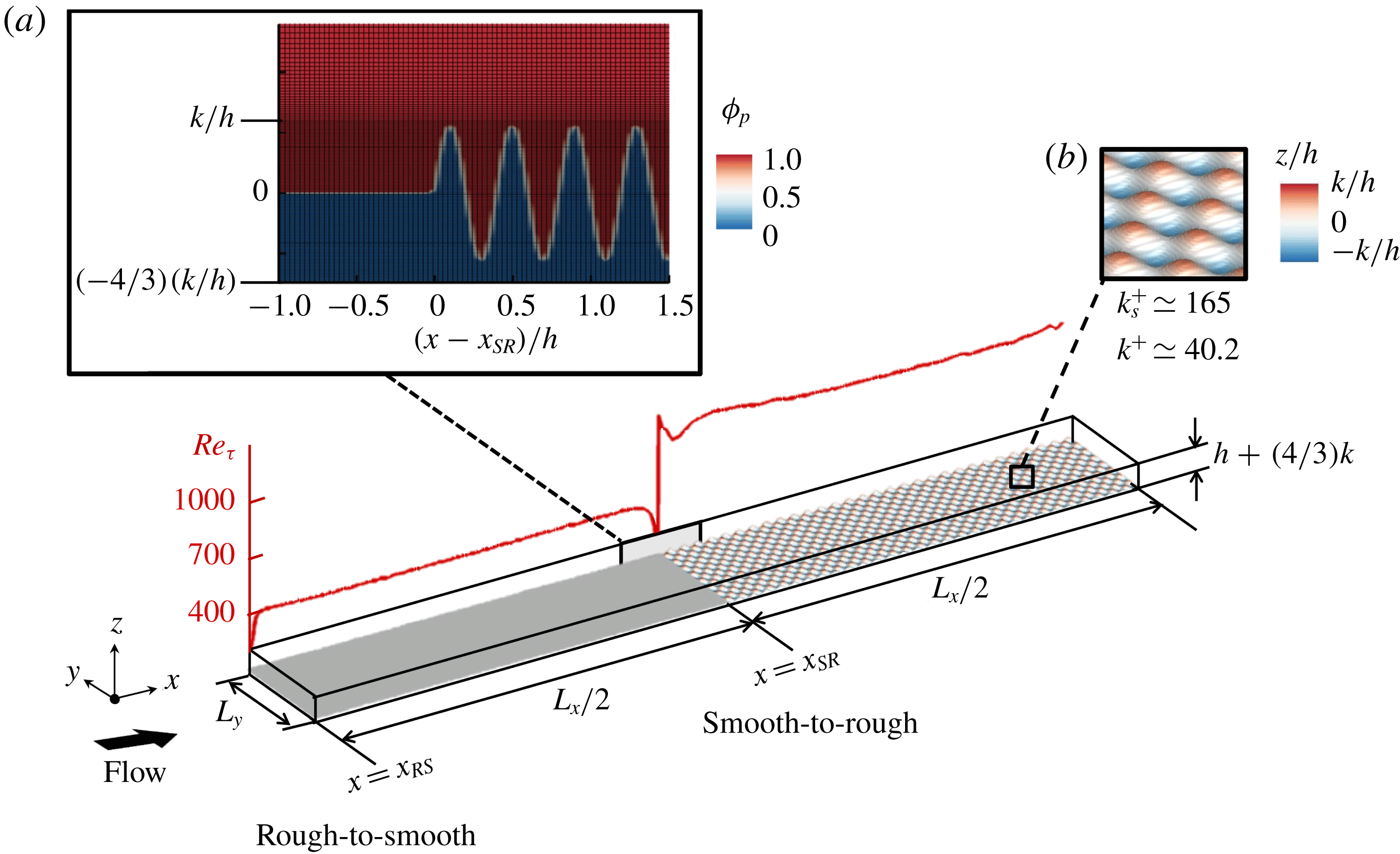
This article aims to address the two above-mentioned aspects. For this purpose, DNS of open-channel flow are performed with a bottom wall equally paved with smooth and rough patches. The presented DNS differ from Lee (Reference Lee2015) and Ismail et al. (Reference Ismail, Zaki and Durbin2018) in two aspects. First, the roughness here is a three-dimensional sinusoidal wall with the mean roughness height aligned with the smooth patch (figure 2). In Lee (Reference Lee2015) and Ismail et al. (Reference Ismail, Zaki and Durbin2018) roughness is made of square bars with the mean height above the smooth patch. Second, here with the streamwise periodicity both rough-to-smooth and smooth-to-rough step changes are studied simultaneously. In contrast, Lee (Reference Lee2015) only considered a smooth-to-rough step change, and Ismail et al. (Reference Ismail, Zaki and Durbin2018) only considered a rough-to-smooth step change. After describing the DNS set-up (§ 2), the results section starts with the domain-length study (§ 3.1). Then, the equilibrium assumption is investigated (§ 3.2). Finally, the definitions of
 $\unicode[STIX]{x1D6FF}_{i}$
are thoroughly studied to search for the most physically consistent choice (§ 3.3).
2 Direct numerical simulation
The continuity and Navier–Stokes equations are solved in this study:
 $$\begin{eqnarray}\frac{\unicode[STIX]{x2202}u_{i}}{\unicode[STIX]{x2202}x_{i}}=0,\quad \frac{\unicode[STIX]{x2202}u_{i}}{\unicode[STIX]{x2202}t}+\frac{\unicode[STIX]{x2202}u_{i}u_{j}}{\unicode[STIX]{x2202}x_{j}}=G\unicode[STIX]{x1D6FF}_{i1}-\frac{1}{\unicode[STIX]{x1D70C}}\frac{\unicode[STIX]{x2202}\widetilde{p}}{\unicode[STIX]{x2202}x_{i}}+\unicode[STIX]{x1D708}\frac{\unicode[STIX]{x2202}^{2}u_{i}}{\unicode[STIX]{x2202}x_{j}^{2}},\end{eqnarray}$$
where
 $x_{1},x_{2}$
and
 $x_{3}$
(or
 $x$
,
 $y$
and
 $z$
) are the streamwise, spanwise and wall-normal directions corresponding to the velocity components
 $u_{1},u_{2}$
and
 $u_{3}$
(or
 $u$
,
 $v$
and
 $w$
), respectively. The pressure gradient
 $\unicode[STIX]{x2202}p/\unicode[STIX]{x2202}x_{i}$
has been decomposed into the constant volume and time-averaged driving part
 $-\unicode[STIX]{x1D70C}G$
, and the periodic part
 $\unicode[STIX]{x2202}\widetilde{p}/\unicode[STIX]{x2202}x_{i}$
.
Computational domain equally divided between the smooth and rough patches. The bottom solid surface is identified with iso-surface of
 $\unicode[STIX]{x1D719}_{p}=0.5$
. Here
 $\unicode[STIX]{x1D719}_{p}$
is the volume of fluid for the pressure cells (appendix A). (a) Side view of the domain, at the smooth-to-rough surface change overlaid by the grid. (b) The roughness elements, coloured by
 $z/h$
. The red curve is the friction Reynolds number
 $Re_{\unicode[STIX]{x1D70F}}\equiv u_{\unicode[STIX]{x1D70F}}h/\unicode[STIX]{x1D708}$
based on the local
 $u_{\unicode[STIX]{x1D70F}}$
.
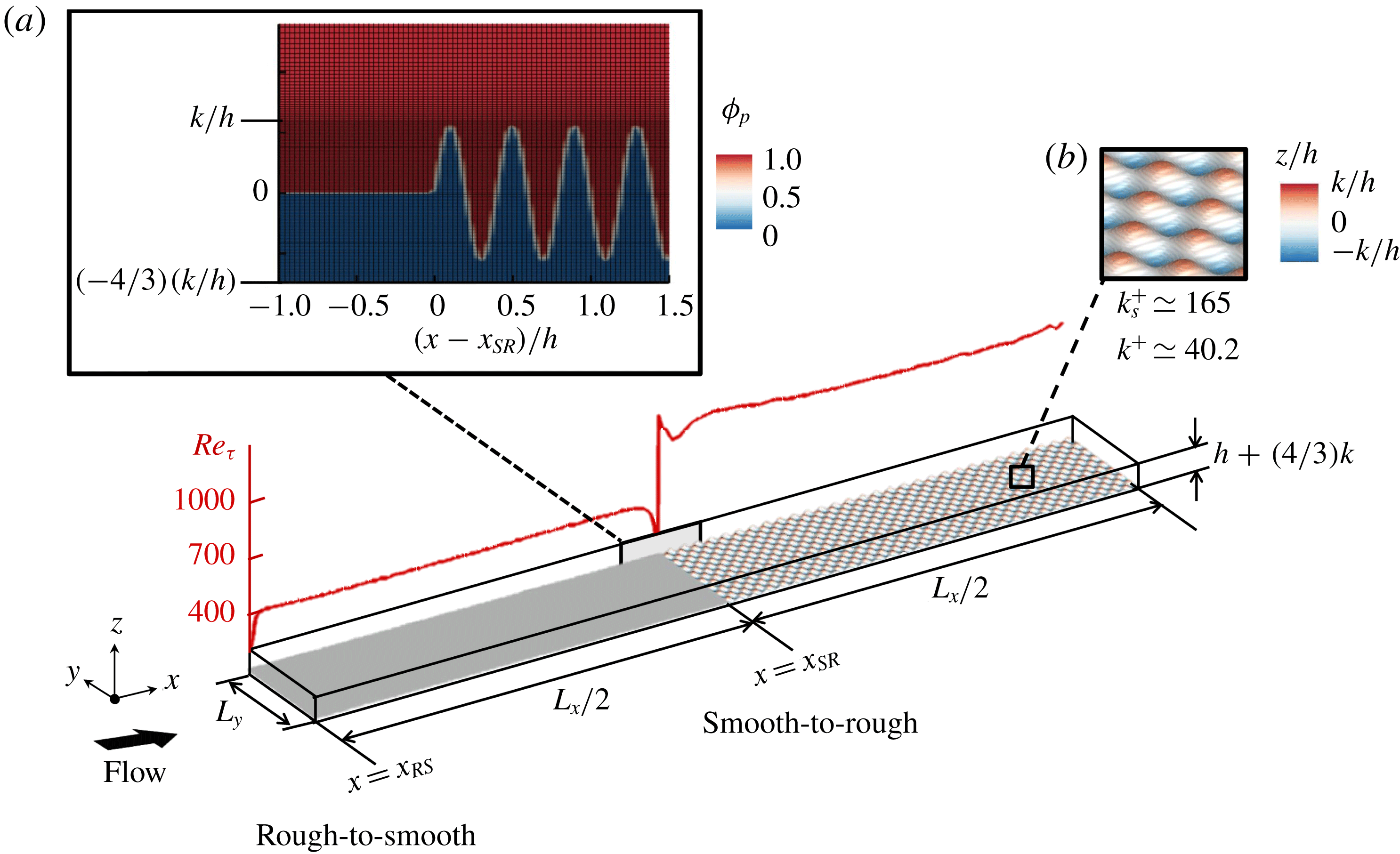
Open-channel flow is the computational domain (figure 2). The bottom surface is equally divided between the smooth and rough patches. The smooth surface is aligned with the mean roughness height (figure 2
a), and the
 $z$
-coordinate origin is placed at the aligned height. The distance between the aligned height and the top boundary is denoted by
 $h$
. Periodic boundary conditions are imposed in the streamwise and spanwise directions. No-slip boundary condition is imposed on the bottom surface through an immersed boundary method (IBM; appendix A) and free-slip boundary condition is imposed on the top boundary. Parameter
 $G$
in (2.1b
) is chosen such that the global Reynolds number
 $Re_{\unicode[STIX]{x1D70F}_{o}}\equiv u_{\unicode[STIX]{x1D70F}_{o}}h/\unicode[STIX]{x1D708}=590$
, where
 $u_{\unicode[STIX]{x1D70F}_{o}}$
is the friction velocity based on the total bottom wall drag, averaged over time and the entire bottom surface. Similar to a homogeneous channel flow,
 $G=u_{\unicode[STIX]{x1D70F}_{o}}^{2}/h$
. However, local
 $Re_{\unicode[STIX]{x1D70F}}\equiv u_{\unicode[STIX]{x1D70F}}h/\unicode[STIX]{x1D708}$
(based on local
 $u_{\unicode[STIX]{x1D70F}}$
) varies from about
 $700$
over the rough patch to about 430 over the smooth patch (figure 2). The local
 $u_{\unicode[STIX]{x1D70F}}$
accounts for both the viscous and form (pressure) drags, which is calculated by integrating the IBM force (appendix A). The bulk velocity is constant in each streamwise location. Therefore, the rough patch exerts a larger drag (larger
 $u_{\unicode[STIX]{x1D70F}}$
) than the smooth patch. In other words,
 $Re_{\unicode[STIX]{x1D70F}}>590$
over the rough patch and
 $Re_{\unicode[STIX]{x1D70F}}<590$
over the smooth patch.
The rough patch (figure 2
b) is made of ‘egg-carton’ roughness (Chan et al.
Reference Chan, MacDonald, Chung, Hutchins and Ooi2015; Chung et al.
Reference Chung, Chan, MacDonald, Hutchins and Ooi2015). The roughness surface
 $z_{r}$
is the following sinusoidal function:
 $$\begin{eqnarray}z_{r}=k\cos (2\unicode[STIX]{x03C0}x/\unicode[STIX]{x1D706})\cos (2\unicode[STIX]{x03C0}y/\unicode[STIX]{x1D706}),\end{eqnarray}$$
where
 $k=0.056h$
and
 $\unicode[STIX]{x1D706}=7.1k$
are the roughness height and wavelength, respectively. For the ‘egg-carton’ roughness, Chan et al. (Reference Chan, MacDonald, Chung, Hutchins and Ooi2015) found that the mean roughness height is an appropriate choice for the virtual origin. Furthermore, Chan et al. (Reference Chan, MacDonald, Chung, Hutchins and Ooi2015) and Chung et al. (Reference Chung, Chan, MacDonald, Hutchins and Ooi2015), by fitting the data of this roughness geometry in the fully rough regime, obtained the equivalent sand-grain roughness
 $k_{s}\simeq 4.1k$
. Therefore, with the current set-up, the flow falls into the fully rough regime over the rough patch,
 $k_{s}^{+}\simeq 165$
. For further information on the geometric characteristics of this type of roughness, the reader is referred to table 2 of Chan et al. (Reference Chan, MacDonald, Chung, Hutchins and Ooi2015).
Equations (2.1a,b ) are integrated in time using the fractional-step algorithm (Perot Reference Perot1993). The time-marching scheme is the third-order Runge–Kutta (Spalart, Moser & Rogers Reference Spalart, Moser and Rogers1991). Spatial discretisation is the fully conservative fourth-order symmetry-preserving scheme of Verstappen & Veldman (Reference Verstappen and Veldman2003). Appendix A contains details of the numerical scheme, IBM and verification against a body-conforming grid solver.
Domain size and grid resolution information. For all cases
 $Re_{\unicode[STIX]{x1D70F}_{o}}=590$
(based on the global
 $u_{\unicode[STIX]{x1D70F}_{o}}$
and
 $h$
) and
 $L_{y}/h=3.1808$
. Parameters
 $\unicode[STIX]{x1D6E5}_{x_{s}}^{+},\unicode[STIX]{x1D6E5}_{y_{s}}^{+}$
and
 $\unicode[STIX]{x1D6E5}_{z_{s}}^{+}|_{0}$
are scaled by
 $u_{\unicode[STIX]{x1D70F}}$
at a fetch of
 $2h$
over the smooth patch. Parameters
 $\unicode[STIX]{x1D6E5}_{x_{r}}^{+},\unicode[STIX]{x1D6E5}_{y_{r}}^{+}$
and
 $\unicode[STIX]{x1D6E5}_{z_{r}}^{+}|_{0}$
are scaled by
 $u_{\unicode[STIX]{x1D70F}}$
at a fetch of
 $2h$
over the rough patch. Here
 $\unicode[STIX]{x1D6E5}_{z_{s}}^{+}|_{0},\unicode[STIX]{x1D6E5}_{z_{r}}^{+}|_{0}$
are the near-wall
 $\unicode[STIX]{x0394}z^{+}$
at
 $z=0$
. Parameters
 $\unicode[STIX]{x1D706}/\unicode[STIX]{x1D6E5}_{x}$
and
 $\unicode[STIX]{x1D706}/\unicode[STIX]{x1D6E5}_{y}$
indicate the number of grid points per roughness wavelength in the streamwise and spanwise directions, respectively.

Three cases are considered whose domain sizes and grid resolutions are listed in table 1. For these cases all the input parameters are the same except the domain lengths (
 $6h,12h$
and
 $24h$
). Uniform grid spacing is used in the streamwise and spanwise directions. For the wall-normal grid, a uniform distribution with
 $\unicode[STIX]{x1D6E5}_{z}u_{\unicode[STIX]{x1D70F}_{o}}/\unicode[STIX]{x1D708}=0.35$
is generated up to the roughness crest, and then is stretched up to the top boundary in a tangent-hyperbolic mapping (figure 2
a). The grid sizes are normalised by the local
 $u_{\unicode[STIX]{x1D70F}}$
at a fetch of
 $2h$
over the smooth patch (
 $\unicode[STIX]{x1D6E5}_{x_{s}}^{+},\unicode[STIX]{x1D6E5}_{y_{s}}^{+},\unicode[STIX]{x1D6E5}_{z_{s}}^{+}|_{0}$
) and at a fetch of
 $2h$
over the rough patch (
 $\unicode[STIX]{x1D6E5}_{x_{r}}^{+},\unicode[STIX]{x1D6E5}_{y_{r}}^{+},\unicode[STIX]{x1D6E5}_{z_{r}}^{+}|_{0}$
). The reason for measuring the resolution at a distance of
 $2h$
is the small variation in the local
 $u_{\unicode[STIX]{x1D70F}}$
(less than 6 %) beyond a fetch of
 $2h$
. The choices of the resolutions in table 1 are from various verification studies (appendix A).
To ease the discussion, the
 $x$
-coordinate at the rough-to-smooth step change is
 $x_{RS}$
and at the smooth-to-rough step change is
 $x_{SR}$
(figure 2). The statistics over the smooth patch are averaged over time and spanwise directions. Over the rough patch, first the statistics are averaged over time and spanwise directions, considering only the in-fluid cells. Then they are streamwise-averaged from a distance of
 $\unicode[STIX]{x1D706}/2$
upstream to
 $\unicode[STIX]{x1D706}/2$
downstream. For locations with distances less than
 $\unicode[STIX]{x1D706}/2$
to
 $x_{SR}$
or
 $x_{RS}$
, the averaging window is constrained by the distance to
 $x_{SR}$
or
 $x_{RS}$
. Throughout this article
 $U,W$
and
 $P$
denote the streamwise and wall-normal mean velocities and mean pressure, respectively. Parameters
 $u_{rms},v_{rms}$
and
 $w_{rms}$
are the r.m.s. of streamwise, spanwise and wall-normal fluctuating velocities, respectively. All these statistics are averaged following the described procedure. Also
 $\langle .\rangle$
by default denotes the same averaging procedure (i.e.
 $\langle u\rangle =U$
), unless it appears with a subscript (i.e.
 $\langle u\rangle _{t}$
is time-averaged
 $u$
). All the parameters in plus units
 $(.)^{+}$
are normalised by the local
 $u_{\unicode[STIX]{x1D70F}}$
and
 $\unicode[STIX]{x1D708}$
(where
 $u_{\unicode[STIX]{x1D70F}}$
is averaged following the averaging procedure described).
3 Results
The results are presented in three subsections. In § 3.1 the parameters of interest are shown insensitive to the domain length and streamwise periodicity. In § 3.2 the equilibrium assumption and its range of validity are studied. Finally, in § 3.3 definitions of
 $\unicode[STIX]{x1D6FF}_{i}$
are studied to find the most physical choice.
3.1 Domain-length effect
In the streamwise-varying roughness, flow recovery is slow (§ 3.2). Full recovery is reached after a fetch of
 $64h$
(Saito & Pullin Reference Saito and Pullin2014). Consequently, the previous wind tunnel experiments (Antonia & Luxton Reference Antonia and Luxton1971; Hanson & Ganapathisubramani Reference Hanson and Ganapathisubramani2016) or DNS studies (Lee Reference Lee2015; Ismail et al.
Reference Ismail, Zaki and Durbin2018) do not reach full recovery due to development lengths that are less than
 $20\unicode[STIX]{x1D6FF}$
(or
 $20h$
). However, full recovery is not the focus of this study. The focus here is on the flow within the IBL in the near field of the surface transition. Given the finite patch length and streamwise periodicity, the unrecovered flow prior to the surface change will in general influence the downstream flow. However, Bou-Zeid, Meneveau & Parlange (Reference Bou-Zeid, Meneveau and Parlange2005) also simulated step changes in a periodic open-channel set-up to replicate the measurements of Bradley (Reference Bradley1968). They argued that the near-wall flow (within the IBL) was insensitive to domain periodicity. Here, this insensitivity is verified by comparing the three domain lengths of table 1. Additionally, in appendix B the case of
 $12h$
is compared with a non-periodic rough-to-smooth case, where fully recovered flow over a rough wall is imposed to the inlet, at the beginning of the smooth patch.
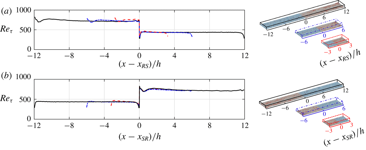
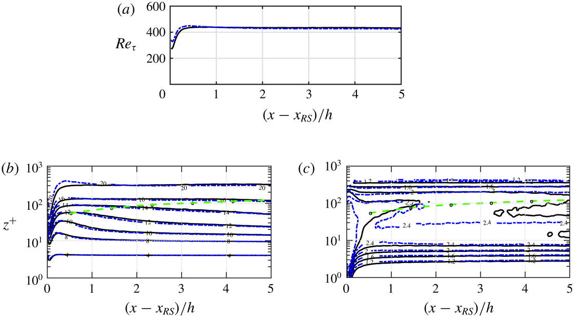
The patch-length effect on
 $Re_{\unicode[STIX]{x1D70F}}$
is studied over the smooth patch (figure 3
a) and the rough patch (figure 3
b). The origin has been placed at the beginning of the corresponding patch, to better isolate the domain-length effect. Except the shortest domain length (case
 $6h$
), the two longer cases yield almost identical
 $Re_{\unicode[STIX]{x1D70F}}$
over both the smooth patch (figure 3
a) and the rough patch (figure 3
b). Even the maximum difference between case
 $6h$
and the two longer cases is only 6.7 % (near
 $x_{RS}$
).
Comparison of the local
 $Re_{\unicode[STIX]{x1D70F}}$
between cases
 $6h$
(– – –),
 $12h$
(– - – - –) and
 $24h$
(——), the cases being shown on the right. Comparison over (a) the smooth patch and (b) the rough patch. The
 $x$
-origin is placed at (a)
 $x_{RS}$
and (b)
 $x_{SR}$
.

The patch-length effect on
 $U^{+}$
and
 $u_{rms}^{+}$
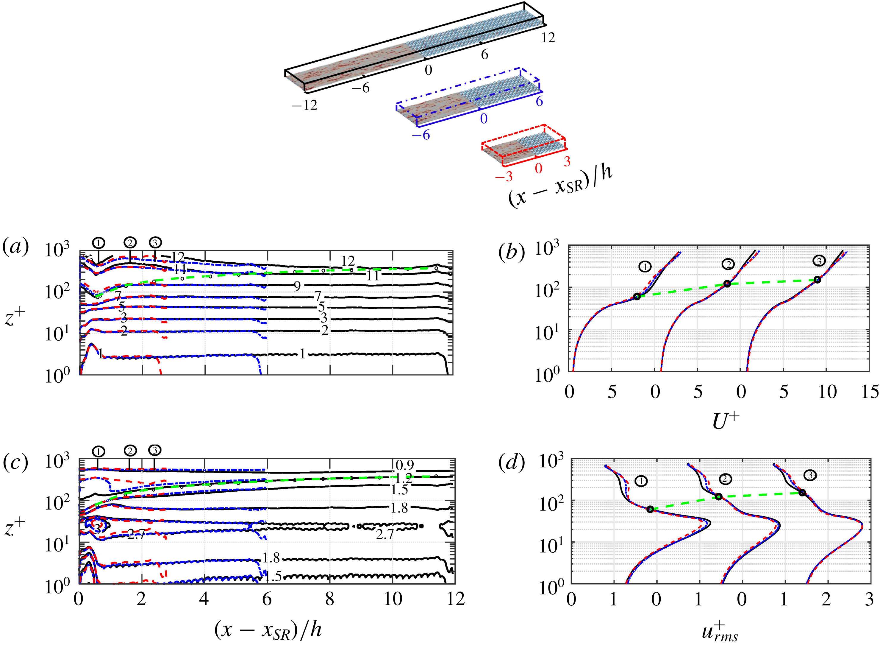
is studied over the smooth patch (figure 4) and the rough patch (figure 5). The IBL thickness
 $\unicode[STIX]{x1D6FF}_{E}$
(– – ○ – –) (defined by Elliott (Reference Elliott1958) and discussed in § 3.3) has been overlaid on the contour lines. Within the IBL, cases
 $12h$
and
 $24h$
yield almost identical
 $U^{+}$
and
 $u_{rms}^{+}$
. This is better demonstrated by comparing the
 $U^{+}$
and
 $u_{rms}^{+}$
profiles up to a fetch of
 $2.5h$
over the smooth patch (figure 4
b,d) and over the rough patch (figure 5
b,d). Within the IBL, the maximum difference between cases
 $12h$
and
 $24h$
in the
 $U^{+}$
profiles is 1 % over both the smooth patch (figure 4
b) and the rough patch (figure 5
b). Within the IBL, the maximum difference in the
 $u_{rms}^{+}$
profiles is 4 % over the smooth patch (figure 4
d) and 1 % over the rough patch (figure 5
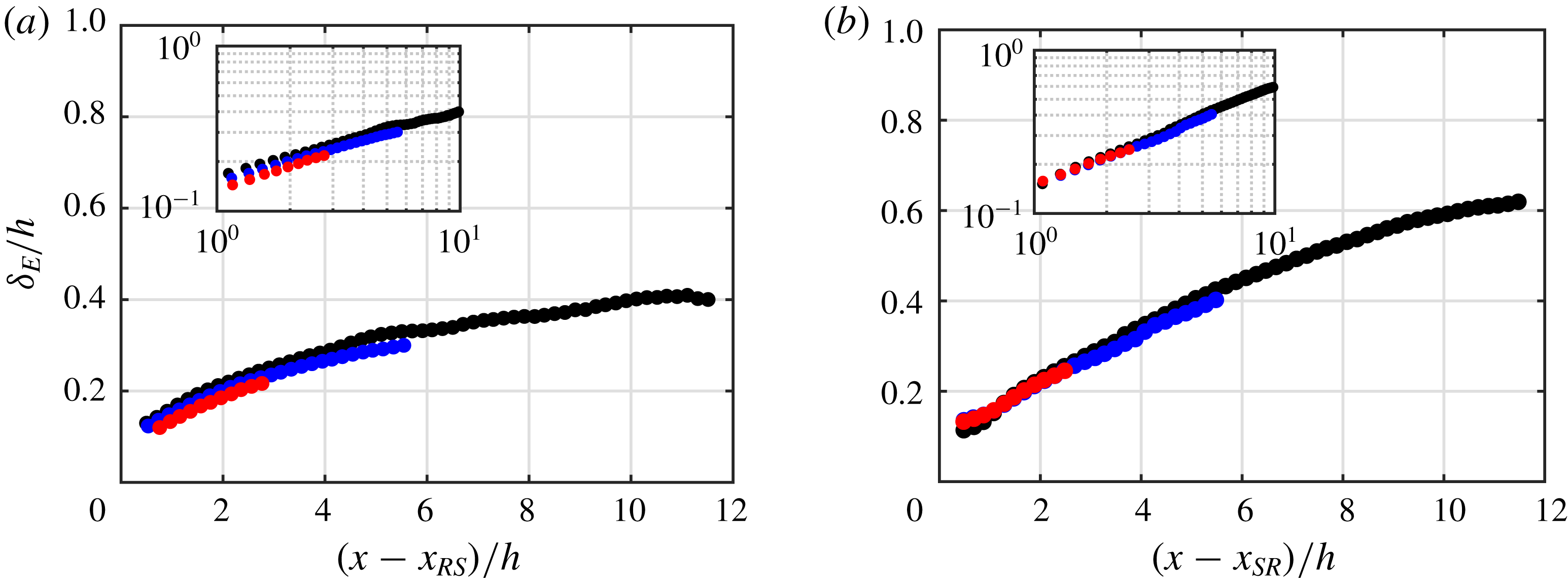
d). As a further support for the small dependence on the domain length, the IBL thicknesses are compared in figure 6. The maximum difference between cases
 $12h$
and
 $24h$
is 5 % over the smooth patch (figure 6
a) and 3 % over the rough patch (figure 6
b). Similar to the findings here, in appendix B negligible difference within the IBL is seen between case
 $12h$
and the non-periodic case; the difference is less than 1 % in
 $U^{+}$
, and 4 % in
 $u_{rms}^{+}$
and
 $Re_{\unicode[STIX]{x1D70F}}$
.
Contour lines of (a)
 $U^{+}$
and (c)
 $u_{rms}^{+}$
for the three domain lengths over the smooth patch. The
 $x$
-origin is placed at
 $x_{RS}$
(consider the top domains). Profiles of (b)
 $U^{+}$
and (d)
 $u_{rms}^{+}$
at several
 $(x-x_{RS})$
:
 $\unicode[STIX]{x2460}$
 $0.5h$
,
 $\unicode[STIX]{x2461}$
 $1.5h$
and
 $\unicode[STIX]{x2462}$
 $2.5h$
. Legends are consistent with those of figure 3. Quantities in plus units are scaled by the local
 $u_{\unicode[STIX]{x1D70F}}$
and
 $\unicode[STIX]{x1D708}$
. The IBL thickness, defined by Elliott (Reference Elliott1958), is overlaid on the contour lines and profiles (– – ○ – –).

Contour lines of (a)
 $U^{+}$
and (c)
 $u_{rms}^{+}$
for the three domain lengths over the rough patch. The
 $x$
-origin is placed at
 $x_{SR}$
(consider the top domains). Profiles of (b)
 $U^{+}$
and (d)
 $u_{rms}^{+}$
at several
 $(x-x_{SR})$
:
 $\unicode[STIX]{x2460}$
 $0.5h$
,
 $\unicode[STIX]{x2461}$
 $1.5h$
and
 $\unicode[STIX]{x2462}$
 $2.5h$
. Legends are consistent with those of figure 3. Quantities in plus units are normalised by the local
 $u_{\unicode[STIX]{x1D70F}}$
and
 $\unicode[STIX]{x1D708}$
. The IBL thickness, defined by Elliott (Reference Elliott1958), is overlaid on the contour lines and profiles (– – ○ – –).
IBL thickness defined by Elliott (Reference Elliott1958) (
 $\unicode[STIX]{x1D6FF}_{E}$
, discussed in § 3.3) over (a) the smooth patch and (b) the rough patch. Cases
 $6h$
(●, red),
 $12h$
(●, blue) and
 $24h$
(●, black). The insets are the same plots using log–log scales.

The identical statistics below
 $\unicode[STIX]{x1D6FF}_{i}$
and the differences above
 $\unicode[STIX]{x1D6FF}_{i}$
are justifiable through the IBL concept: a layer that is influenced by the surface underneath. Below
 $\unicode[STIX]{x1D6FF}_{i}$
, the flow ignores its history from the upstream surfaces. Therefore, it has minimal dependence on the patch length. Above
 $\unicode[STIX]{x1D6FF}_{i}$
, however, the flow carries its history from upstream surfaces. Therefore, it depends on the patch length. This section and appendix B show that with domain lengths of at least
 $12h$
(
 $6h$
for each patch), the flow inside the IBL remains insensitive to the patch length and streamwise periodicity. The results reported in the rest of this paper are from the longest case (case
 $24h$
).
Variations of (a)
 $U/U_{b}$
, (b)
 $(h/U_{b})(\unicode[STIX]{x2202}U/\unicode[STIX]{x2202}x)$
, (c)
 $[h/(\unicode[STIX]{x1D70C}U_{b}^{2})](\unicode[STIX]{x2202}P/\unicode[STIX]{x2202}x)$
, (d)
 $W/U_{b}$
and (e,f)
 $u_{rms}/U_{b}$
, scaled by the bulk velocity
 $U_{b}$
and
 $h$
. The regions over the smooth patch (S1 + S2) and rough patch (R1 + R2) are separated into zones S1 and R1 that cover a fetch of
 $2h$
, and zones S2 and R2 that cover the remaining portions. The fields are overlaid by the spanwise projection of the roughness, in black colour. In (c) the total pressure gradient
 $\unicode[STIX]{x2202}P/\unicode[STIX]{x2202}x$
includes the driving
 $-\unicode[STIX]{x1D70C}G$
and periodic
 $\unicode[STIX]{x2202}\widetilde{P}/\unicode[STIX]{x2202}x$
parts. In (f) the
 $z$
-axis is in log scale to highlight the near-wall region. The outer peak of
 $u_{rms}$
over the smooth patch is marked with (– – –).

3.2 Equilibrium assumption
In this subsection validity of the equilibrium assumption is examined. First, the overall flow behaviour is described (figure 7). The quantities are scaled by the bulk velocity
 $U_{b}\simeq 12.78u_{\unicode[STIX]{x1D70F}_{o}}$
and channel height
 $h$
. For ease of discussion, each patch is divided into two zones: S1 and S2 over the smooth patch, and R1 and R2 over the rough patch. Zones S1 and R1 cover up to a fetch of
 $2h$
, where the flow variations are rapid. Zones S2 and R2 cover the remaining portions, where the flow variations are more gradual. As a measure of the flow acceleration or deceleration,
 $(h/U_{b})(\unicode[STIX]{x2202}U/\unicode[STIX]{x2202}x)$
is plotted in figure 7(b). In figure 7(c) the pressure gradient
 $\unicode[STIX]{x2202}P/\unicode[STIX]{x2202}x$
includes both the driving part (
 $-\unicode[STIX]{x1D70C}G$
) and the periodic part (
 $\unicode[STIX]{x2202}\widetilde{P}/\unicode[STIX]{x2202}x$
). During the step change the periodic
 $\unicode[STIX]{x2202}\widetilde{P}/\unicode[STIX]{x2202}x$
becomes an order of magnitude larger than the driving
 $-\unicode[STIX]{x1D70C}G$
. In other words,
 $hG/U_{b}^{2}\simeq 6\times 10^{-3}$
which is not visible with the colour range in figure 7(c).
In figure 7(b) following the rough-to-smooth step change the near-wall flow accelerates, while away from the wall the flow decelerates. This is because
 $\text{d}U_{b}/\text{d}x=\int _{0}^{h}(\unicode[STIX]{x2202}U/\unicode[STIX]{x2202}x)\,\text{d}z=0$
, and
 $\unicode[STIX]{x2202}U/\unicode[STIX]{x2202}x>0$
near the wall must be accompanied by
 $\unicode[STIX]{x2202}U/\unicode[STIX]{x2202}x<0$
away from the wall. Simultaneously, the flow is exposed to an adverse pressure gradient (APG) (
 $\unicode[STIX]{x2202}P/\unicode[STIX]{x2202}x>0$
), which becomes strong at the beginning of zone S1 (figure 7
c). Following the smooth-to-rough step change, the acceleration/deceleration mechanism is reversed: the near-wall flow decelerates while the outer one accelerates, and the flow is exposed to a favourable pressure gradient. In figure 7(d) immediately downstream of the rough-to-smooth step change (zone S1), the wall-normal flow direction is downward (
 $W<0$
), while immediately downstream of the smooth-to-rough step change (zone R1), the wall-normal flow direction is upward (
 $W>0$
). This behaviour is justifiable through the continuity equation,
 $\unicode[STIX]{x2202}U/\unicode[STIX]{x2202}x+\unicode[STIX]{x2202}W/\unicode[STIX]{x2202}z=0$
. In zone S1,
 $\unicode[STIX]{x2202}U/\unicode[STIX]{x2202}x>0$
near the wall requires
 $\unicode[STIX]{x2202}W/\unicode[STIX]{x2202}z<0$
, and since
 $W=0$
at the wall,
 $W$
must be negative near the wall. The same analysis justifies positive
 $W$
in zone R1.
Some interesting phenomena are seen in the
 $u_{rms}$
field (figure 7
e,f). Immediately downstream of the rough-to-smooth step change, there is a locally high
 $u_{rms}$
region (at
 $x-x_{SR}\simeq -12h$
and
 $z\simeq 0.05h$
). Along the smooth patch,
 $u_{rms}$
near the wall (
 $z\lesssim 0.5h$
) is decreased, while away from the wall (
 $z>0.5h$
) it preserves its intensity. This leads to formation of an outer peak in the
 $u_{rms}$
field (marked with the dashed magenta curve). Immediately downstream of the smooth-to-rough step change (at
 $x-x_{SR}\simeq 0$
) there is a sudden rise in
 $u_{rms}$
. Along the rough patch the high-intensity
 $u_{rms}$
around the roughness elements gradually propagates to higher
 $z$
distances. These phenomena are further investigated next.
3.2.1 Rough-to-smooth step change
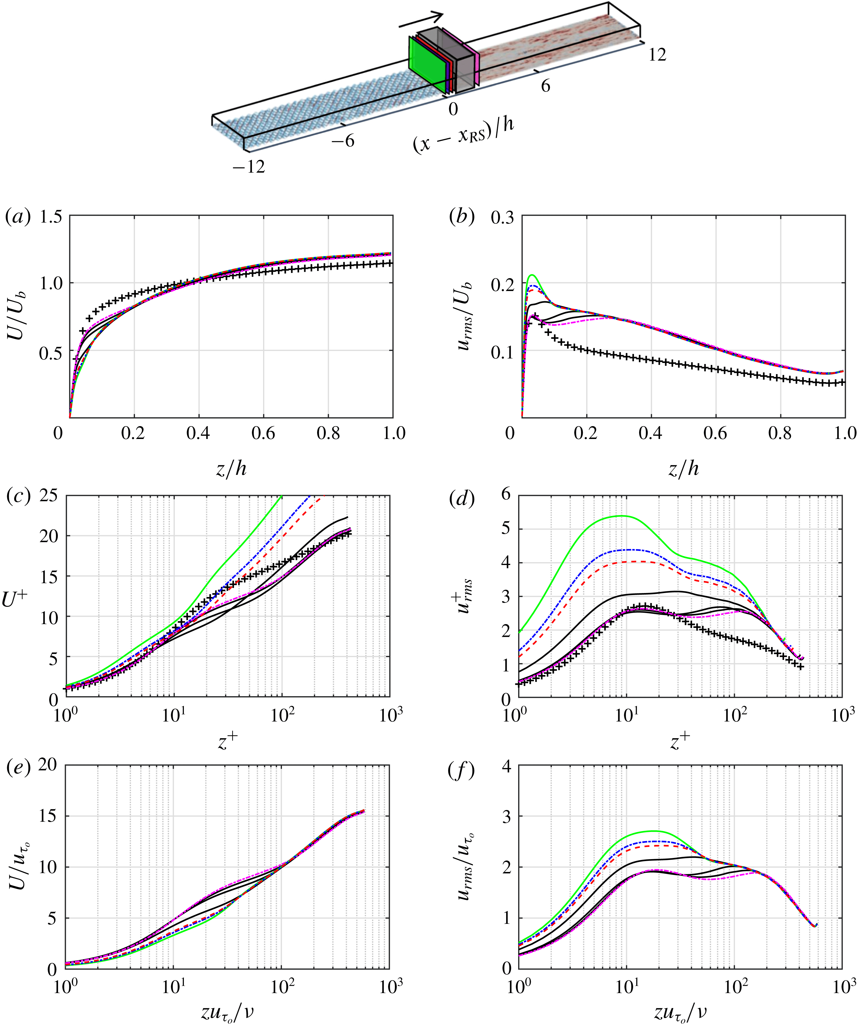
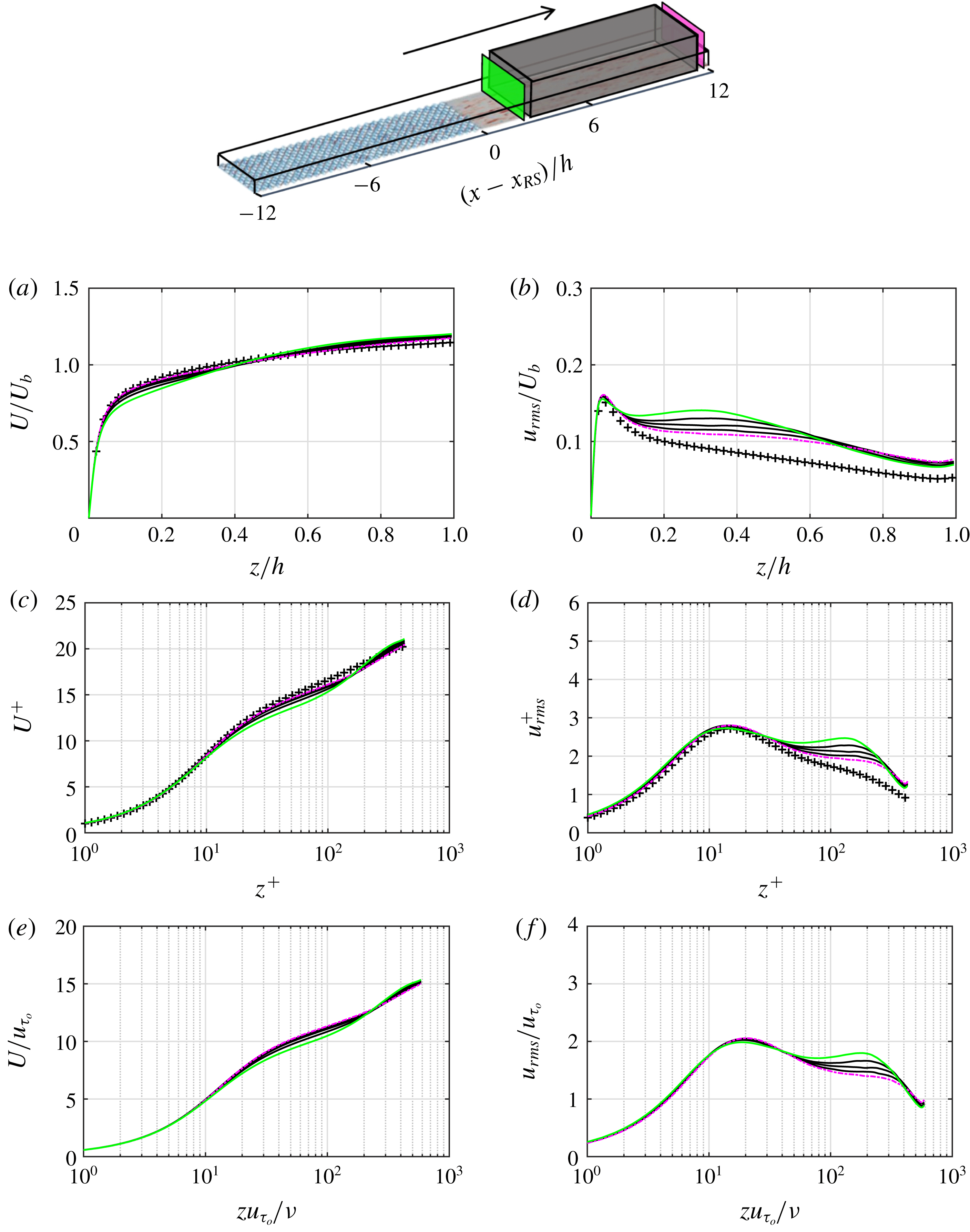
The profiles of
 $U$
and
 $u_{rms}$
up to a fetch of
 $2h$
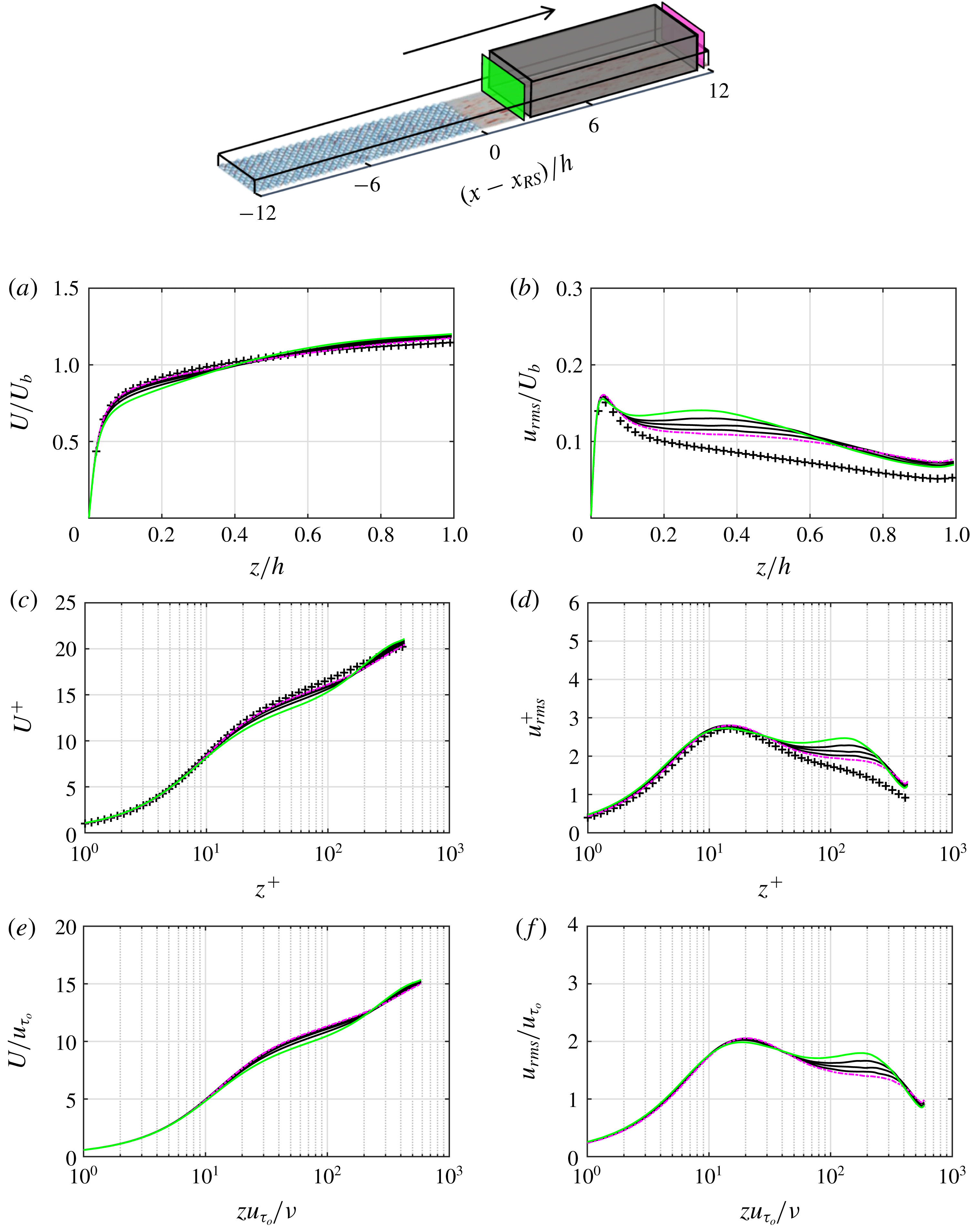
over the smooth patch are shown in figure 8. The profiles are scaled by
 $U_{b}$
and
 $h$
in figure 8(a,b), local
 $u_{\unicode[STIX]{x1D70F}}$
and
 $\unicode[STIX]{x1D708}$
in figure 8(c,d) and
 $u_{\unicode[STIX]{x1D70F}_{o}}$
and
 $\unicode[STIX]{x1D708}$
in figure 8(e,f). Over the smooth patch,
 $Re_{\unicode[STIX]{x1D70F}}$
converges to the asymptotic value of 437. Therefore, to measure the flow distance to equilibrium, a separate simulation of fully developed smooth open-channel flow at
 $Re_{\unicode[STIX]{x1D70F}}=437$
was conducted (
 $L_{x}/h\times L_{y}/h=2\unicode[STIX]{x03C0}\times \unicode[STIX]{x03C0}$
,
 $\unicode[STIX]{x1D6E5}_{x}^{+}\times \unicode[STIX]{x1D6E5}_{y}^{+}\simeq 10.7\times 5.4$
).
Profiles of (a,c,e)
 $U$
and (b,d,f)
 $u_{rms}$
up to a fetch of
 $2h$
over the smooth patch, zone S1. Profiles are normalised by (a,b)
 $U_{b},h$
, (c,d) local
 $u_{\unicode[STIX]{x1D70F}}$
and
 $\unicode[STIX]{x1D708}$
and (e,f)
 $u_{\unicode[STIX]{x1D70F}_{o}}$
and
 $\unicode[STIX]{x1D708}$
. The black curves are equally spaced in the range
 $0.2h\leqslant (x-x_{RS})\leqslant 1.8h$
(the shadowed box at the top). Here
 $(x-x_{RS})=0.05h$
(——),
 $0.08h$
(– - – - –, blue),
 $0.1h$
(– – –) and
 $2h$
(– - – - –, magenta); DNS of fully developed smooth open-channel flow at
 $Re_{\unicode[STIX]{x1D70F}}=437$
(+).

In figure 8(c) the
 $U^{+}$
profiles substantially depart from equilibrium. The departure even propagates down to the buffer and viscous sublayer regions (
 $z^{+}\lesssim 30$
). Due to the thinner buffer layer, a downshift appears in the
 $U^{+}$
profiles. Similar downshift is seen in the APG boundary layers (Nickels Reference Nickels2004). When the APG strength
 $P_{x}^{+}$
,
 $\unicode[STIX]{x1D708}/(\unicode[STIX]{x1D70C}u_{\unicode[STIX]{x1D70F}}^{3})(\unicode[STIX]{x2202}P/\unicode[STIX]{x2202}x)$
, goes beyond 0.005, it breaks the linear viscous sublayer. Here, from the beginning of the smooth patch up to a fetch of
 $2h$
,
 $P_{x}^{+}$
varies from 0.022 to 0.001 (not shown). Therefore, it is possible that APG is causing the downshift in the
 $U^{+}$
profiles. This possibility was examined by reconstructing the
 $U^{+}$
profiles using the obtained
 $P_{x}^{+}$
from DNS, substituted in Nickel’s formulation for the viscous sublayer (
 $U^{+}=z^{+}+1/2P_{x}^{+}z^{+^{2}}+\text{h.o.t}$
) and the log layer ((3.1) in Nickels Reference Nickels2004). At each
 $x$
-location,
 $P_{x}^{+}$
is constant for
 $z^{+}\leqslant 100$
. The reconstructed profiles had a much shallower downshift than what is seen in figure 8(c). Therefore, the downshift is not merely caused by APG.
Profiles of (a)
 $U^{+}$
and (b) its logarithmic slope
 $\unicode[STIX]{x2202}U^{+}/\unicode[STIX]{x2202}\ln (z^{+})$
for case
 $24h$
at
 $(x-x_{RS})=2h$
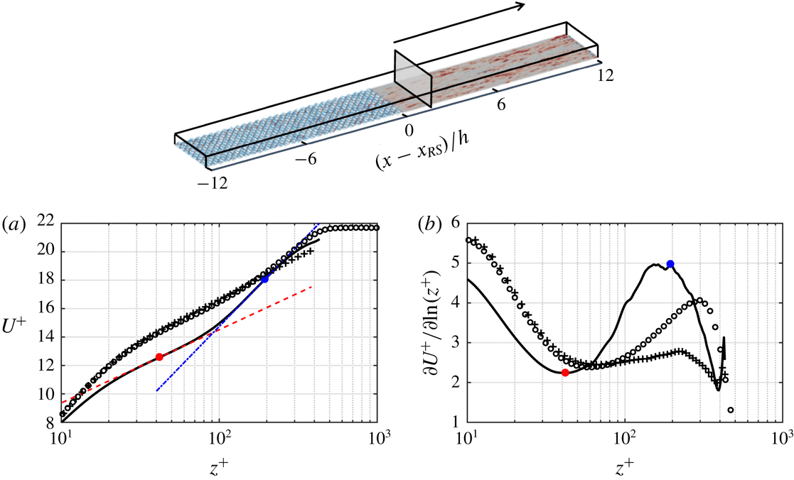
(——), indicated in the top domain. The inner and outer logarithmic slopes are identified through the extrema of
 $\unicode[STIX]{x2202}U^{+}/\unicode[STIX]{x2202}\ln (z^{+})$
(●, red; ●, blue). The fitting lines (– – –) and (– - – - –) have the same slopes as the extrema. Fully developed open-channel flow at
 $Re_{\unicode[STIX]{x1D70F}}=437$
(+). Canonical boundary layer at
 $Re_{\unicode[STIX]{x1D70F}}\simeq 445$
(○) by Jiménez et al. (Reference Jiménez, Hoyas, Simens and Mizuno2010).
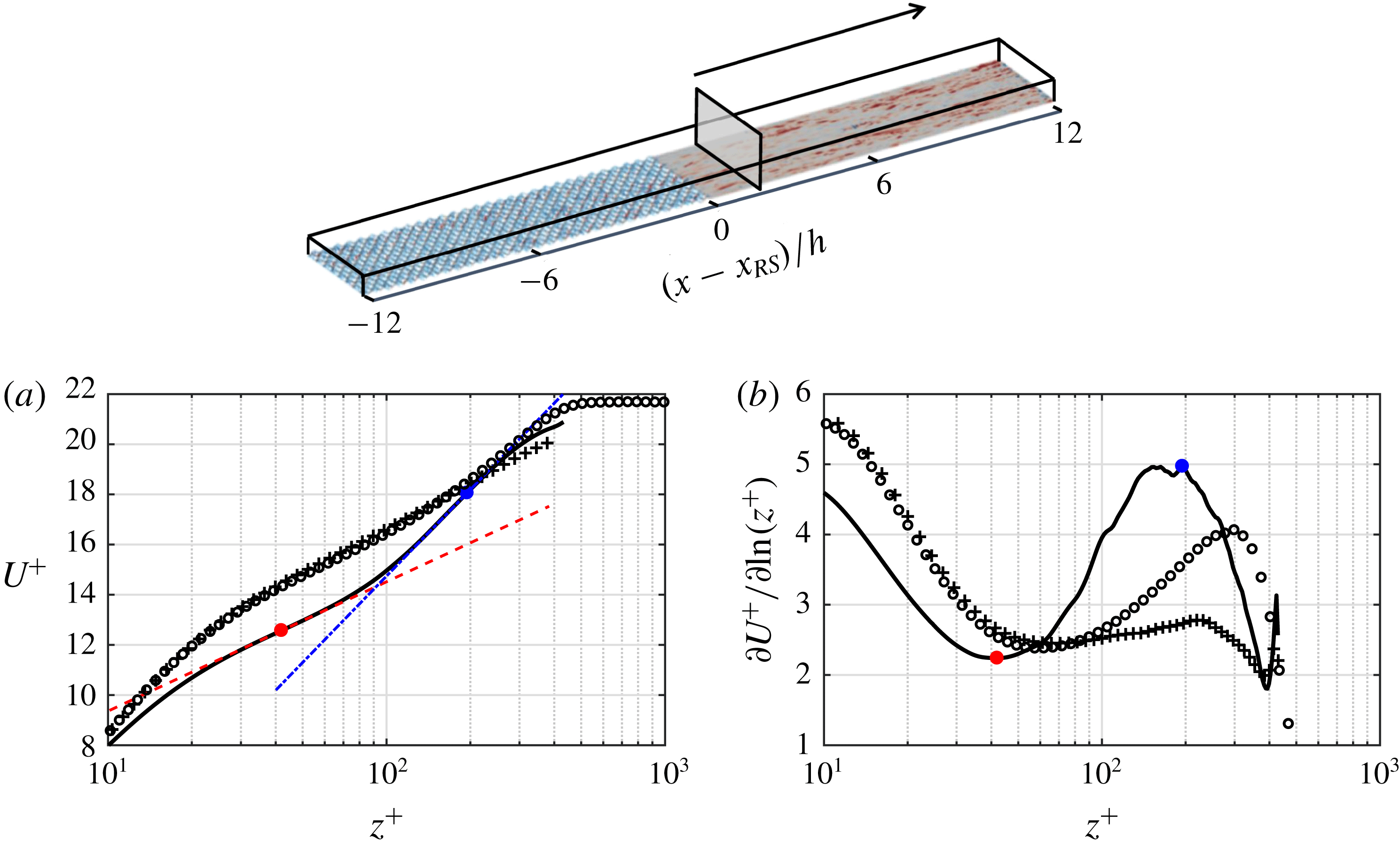
One can also see that there is a change in the logarithmic slope of the
 $U^{+}$
profiles across the channel. This is better demonstrated in figure 9(a) showing the
 $U^{+}$
profile at
 $(x-x_{RS})=2h$
. To detect the slope change, the slope curve
 $\unicode[STIX]{x2202}U^{+}/\unicode[STIX]{x2202}\ln (z^{+})$
at
 $(x-x_{RS})=2h$
(——) is compared with the equilibrium counterpart (+) in figure 9(b). For equilibrium open-channel flow,
 $\unicode[STIX]{x2202}U^{+}/\unicode[STIX]{x2202}\ln (z^{+})$
yields almost a plateau for
 $40\lesssim z^{+}\lesssim 300$
, indicating that the logarithmic region dominates the wake in this range. This is clear when compared to a canonical boundary layer (○) at similarly matched
 $Re_{\unicode[STIX]{x1D70F}}\simeq 445$
(Jiménez et al.
Reference Jiménez, Hoyas, Simens and Mizuno2010), which yields a narrow logarithmic region but a strong outer wake. During the rough-to-smooth step change (——) the slope curve yields a local minimum (●, red) and a local maximum (●, blue) at
 $z^{+}\simeq 40$
and
 $z^{+}\simeq 200$
, indicating the inner and outer logarithmic slopes, respectively. The inner slope reflects the influence of the new smooth surface, while the outer slope owing to the weak channel wake predominantly reflects the flow history from the upstream rough surface. The new surface effect can also be seen in figure 8(e) comparing the
 $U$
profiles with their most upstream counterpart (the green curve). The extent up to which each profile departs from the green curve (which also appears as the inner logarithmic slope) is the result of the new surface underneath.
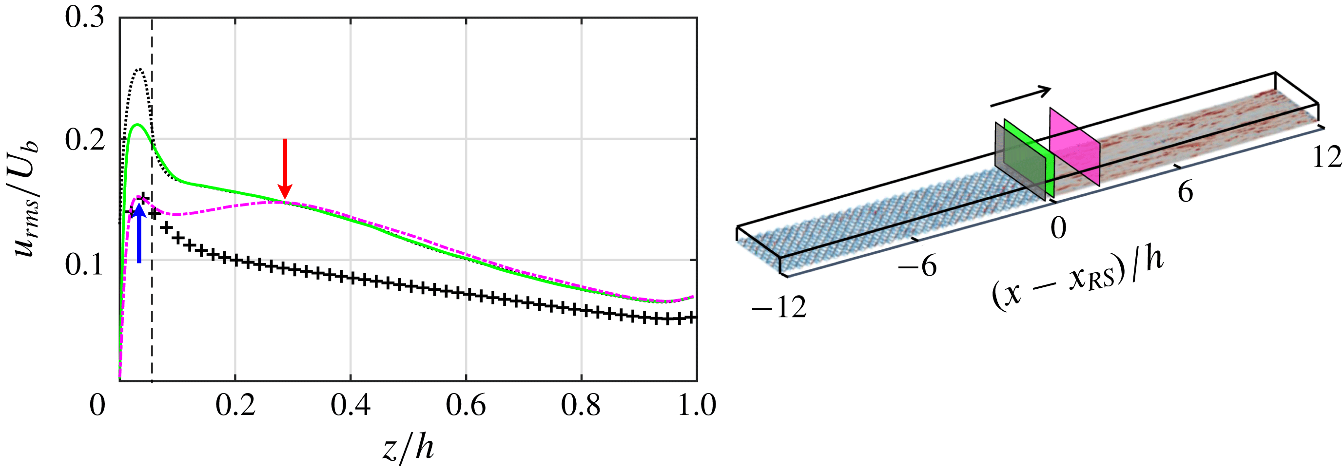
In figure 8(b,d,f) the
 $u_{rms}$
profile at the very beginning of the smooth patch (the green curve at
 $x-x_{RS}=0.05h$
) yields a large inner peak (at
 $z^{+}\simeq 9$
). This peak corresponds to the high near-wall
 $u_{rms}$
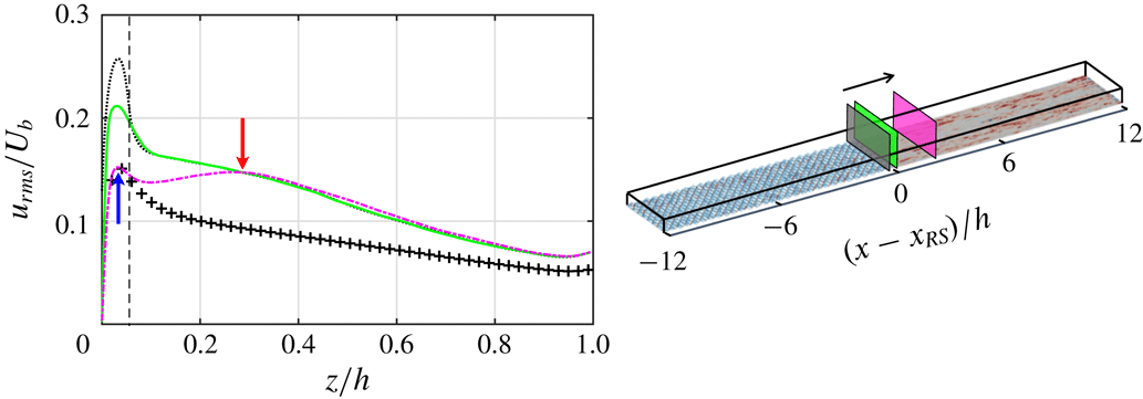
appearing immediately downstream of the rough-to-smooth step change, discussed earlier in figure 7(e,f). It is the remnant of the turbulent fluctuations emanated from the upstream rough patch. This peak is different from the inner peak formed further downstream due to the buffer layer formation (the magenta dashed-dotted curve at
 $z^{+}\simeq 14$
). This is better shown in figure 10, comparing the
 $u_{rms}$
profiles immediately upstream of the rough-to-smooth step change (
 $x-x_{RS}=-0.05h$
) with the profiles immediately downstream of the step change (
 $x-x_{RS}=0.05h$
) and at a fetch of
 $2h$
(
 $x-x_{RS}=2h$
). To make the profiles comparable, they are scaled by
 $U_{b}$
. As is seen, the inner peak immediately downstream of the step change (the green solid curve) is a weakened remnant of the inner peak immediately upstream of the step change (the black dotted curve). Further downstream at
 $(x-x_{RS})=2h$
(the magenta dashed-dotted curve), two different peaks appear which are identified by arrows. The inner peak (the upward arrow) is due to the buffer layer formation, and the outer one (the downward arrow) is due to the surface change. The magenta curve matches the most upstream profile (the green solid curve) beyond the outer peak location. Along the smooth patch the outer peak moves to a higher
 $z$
(figure 8
f), locating the maximum height up to which
 $u_{rms}$
is influenced by the surface underneath. This outer peak is marked with a magenta dashed curve in figure 7(e,f).
Profiles of
 $u_{rms}$
, normalised by
 $U_{b}$
, at
 $(x-x_{RS})=-0.05h$
(- - - -),
 $0.05h$
(——) and
 $2h$
(– - – - –), indicated in the domain on the right. The vertical dashed line locates the roughness crest (
 $z=k$
). The upward and downward arrows indicate the inner and outer peaks of (– - – - –).
Profiles of (a,c,e)
 $U$
and (b,d,f)
 $u_{rms}$
for
 $3h\leqslant (x-x_{RS})\leqslant 11h$
, zone S2. Normalisation is consistent with figure 8. The black curves are equally spaced in the range
 $5h\leqslant (x-x_{RS})\leqslant 9h$
(the shadowed box). Here
 $(x-x_{RS})=3h$
(——) and
 $11h$
(– - – - –). DNS of fully developed smooth open-channel flow at
 $Re_{\unicode[STIX]{x1D70F}}=437$
(+).
The profiles of
 $U$
and
 $u_{rms}$
in the remaining portion of the smooth patch, zone S2, are shown in figure 11. In this figure the
 $x$
-distance between the first and the last profile is four times larger than the one in figure 8. However, the profile variation is much slower. In other words, the recovery for the initial
 $2h$
fetch length is much faster than that for the remaining portion. By the end of the smooth patch, the flow is still not fully recovered. The effect of the upstream rough patch still persists in the
 $u_{rms}$
profile (figure 11
b,d,f), as well as the
 $U$
profile (figure 11
a,c,e).
Summary of flow configuration for case
 $24h$
and rough-to-smooth DNS of Ismail et al. (Reference Ismail, Zaki and Durbin2018). The rough patch Reynolds number
 $Re_{\unicode[STIX]{x1D70F}_{r}}=u_{\unicode[STIX]{x1D70F}_{r}}h/\unicode[STIX]{x1D708}$
is computed at
 $(x-x_{RS})=-h$
, and the smooth patch Reynolds number
 $Re_{\unicode[STIX]{x1D70F}_{s}}=u_{\unicode[STIX]{x1D70F}_{s}}h/\unicode[STIX]{x1D708}$
is computed at
 $(x-x_{RS})=7.5h$
. The arrow indicates the flow direction.

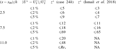
Recovery of
 $U^{+}$
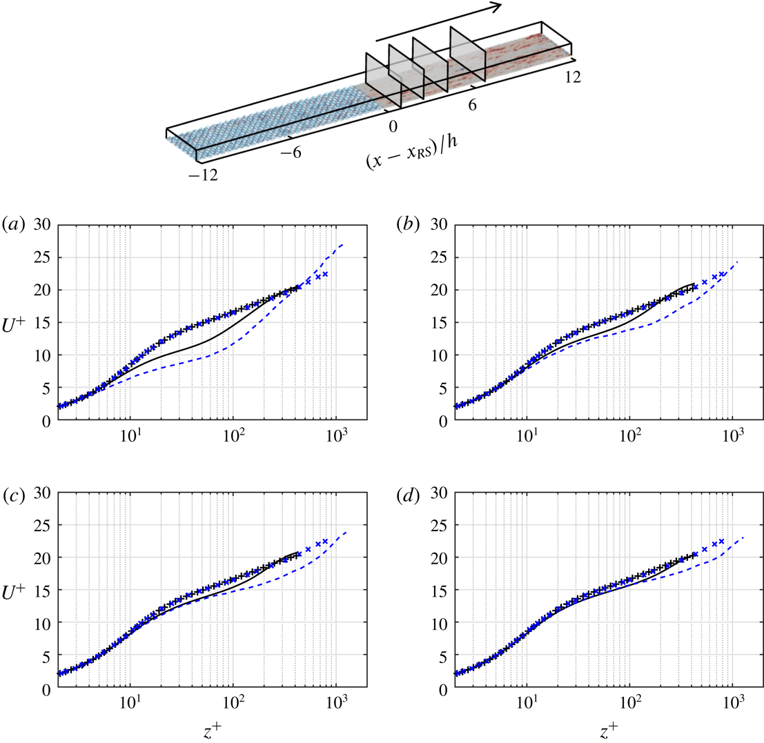
over the smooth patch is compared with the rough-to-smooth DNS of Ismail et al. (Reference Ismail, Zaki and Durbin2018) in figure 12 and table 3. The configuration of Ismail et al. (Reference Ismail, Zaki and Durbin2018) differs from the current case (case
 $24h$
) in several aspects (table 2). These aspects include:
 $Re_{\unicode[STIX]{x1D70F}}$
, roughness shape, roughness size and roughness origin. Considering figure 12, initially at
 $(x-x_{RS})=0.8h$
(figure 12
a) the
 $U^{+}$
profile of Ismail et al. (Reference Ismail, Zaki and Durbin2018) yields a larger departure from equilibrium. Nevertheless, after a fetch of
 $(x-x_{RS})=4.1h$
(figure 12
c) the
 $U^{+}$
profile of both datasets reaches the same recovery level. This is better quantified in table 3, which reports the
 $z^{+}$
up to which
 $U^{+}$
differs from the fully developed profile
 $U_{S}^{+}$
by less than 1 %, 2 % and 5 %. It is seen that the recovered
 $z^{+}$
between case
 $24h$
and Ismail et al. (Reference Ismail, Zaki and Durbin2018) does not change beyond a fetch of
 $(x-x_{RS})=4.1h$
, despite the differences in
 $Re_{\unicode[STIX]{x1D70F}}$
and roughness geometry. This finding is different from the WMLES of Saito & Pullin (Reference Saito and Pullin2014) over rough-to-smooth step change, and vice versa. They showed that varying
 $Re_{\unicode[STIX]{x1D70F}}$
by two orders of magnitude delays the recovery distance of
 $U^{+}$
by two to three times. This difference might be due to the wider range of
 $Re_{\unicode[STIX]{x1D70F}}$
in Saito & Pullin (Reference Saito and Pullin2014) or due to the WMLES, which inherently assumes some degree of equilibrium.
Rough-to-smooth comparison of
 $U^{+}$
profiles between case
 $24h$
(——) and DNS of Ismail et al. (Reference Ismail, Zaki and Durbin2018) (– – –). Comparison is made at the several
 $(x-x_{RS})$
locations (shown in the domain): (a)
 $0.8h$
; (b)
 $2.5h$
; (c)
 $4.1h$
; (d)
 $7.5h$
. Fully recovered flow for case
 $24h$
at
 $Re_{\unicode[STIX]{x1D70F}}=437$
(+) and Ismail et al. (Reference Ismail, Zaki and Durbin2018) at
 $Re_{\unicode[STIX]{x1D70F}}=1115$
(
 $\times$
).

Table 3 shows that the equilibrium assumptions must be applied cautiously over the rough-to-smooth step change. For instance, to predict
 $u_{\unicode[STIX]{x1D70F}}$
by at least 5 % error from the equilibrium profile, the flow must be resolved down to
 $z^{+}\simeq 9$
at a fetch of
 $2.5h$
, and
 $z^{+}\simeq 69$
at a fetch of
 $7.5h$
. Beyond a fetch of
 $11h$
, fitting at any
 $z^{+}$
yields
 $u_{\unicode[STIX]{x1D70F}}$
with less than 5 % error. Note that these findings are based on the processed datasets and may change for other datasets.
Recovery in
 $U^{+}$
of case
 $24h$
and DNS of Ismail et al. (Reference Ismail, Zaki and Durbin2018) after the rough-to-smooth step change. Recovery is measured based on 1 %, 2 % or 5 % difference with the
 $U_{S}^{+}$
profile of fully developed smooth channel. The fully developed case is at
 $Re_{\unicode[STIX]{x1D70F}}=437$
for case
 $24h$
and
 $Re_{\unicode[STIX]{x1D70F}}=1115$
for Ismail et al. (Reference Ismail, Zaki and Durbin2018).

3.2.2 Smooth-to-rough step change
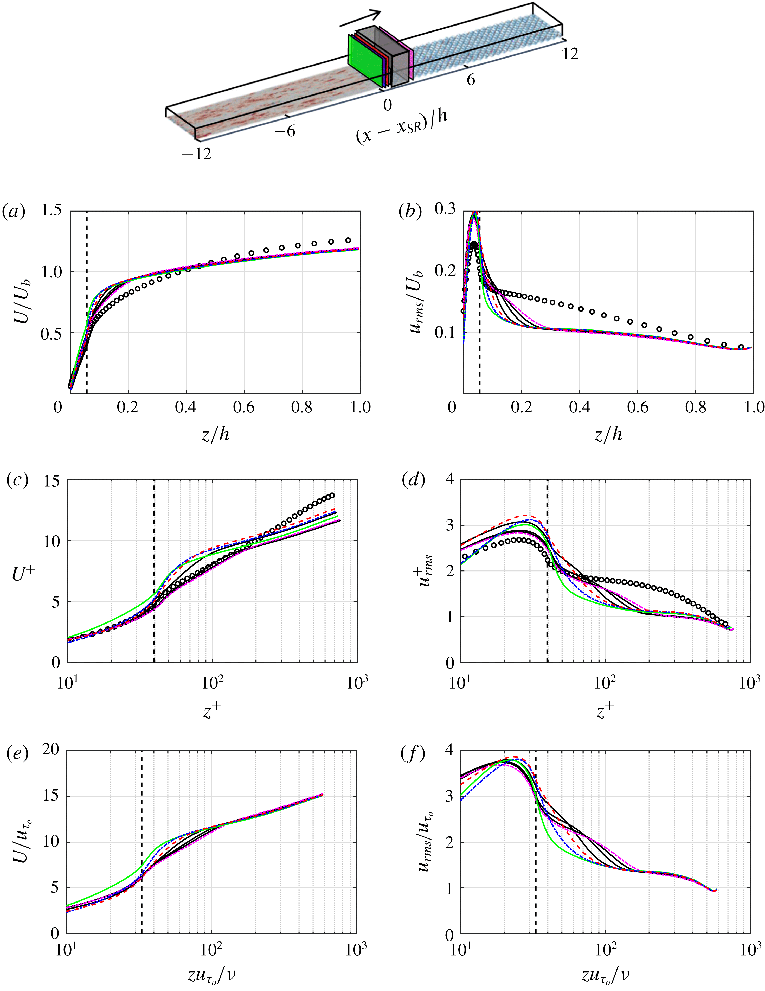
Figure 13 shows the profiles of
 $U$
and
 $u_{rms}$
up to a fetch of
 $2h$
over the rough patch, zone R1. To measure the flow recovery, the profiles are compared against the DNS of homogeneous ‘egg-carton’ rough open-channel flow, with
 $k/h=0.056$
at the expected fully recovered flow condition over the rough patch (
 $Re_{\unicode[STIX]{x1D70F}}=704$
,
 $L_{x}/h\times L_{y}/h\simeq 5.97\times 3.18$
,
 $\unicode[STIX]{x1D6E5}_{x}^{+}\times \unicode[STIX]{x1D6E5}_{y}^{+}\simeq 10.9\times 5.8$
).
Profiles of (a,c,e)
 $U$
and (b,d,f)
 $u_{rms}$
up to a fetch of
 $2h$
over the rough patch, zone R1. Normalisation is consistent with figure 8. The vertical dashed line locates the roughness crest. The black curves are equally spaced in the range
 $0.8h\leqslant (x-x_{SR})\leqslant 1.8h$
,
 $(x-x_{SR})=0.2h$
(——),
 $0.4h$
(– - – - –, blue),
 $0.6h$
(– – –) and
 $2h$
(– - – - –, magenta). Fully developed open channel over homogeneous ‘egg-carton’ roughness (○), with
 $k/h=0.056$
at
 $Re_{\unicode[STIX]{x1D70F}}=704$
.

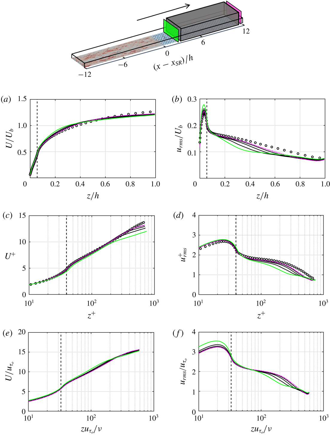
Profiles of (a,c,e)
 $U$
and (b,d,f)
 $u_{rms}$
for
 $3h\leqslant (x-x_{SR})\leqslant 11h$
, zone R2. Normalisation is consistent with figure 8. The black curves are equally spaced in the range
 $5h\leqslant (x-x_{SR})\leqslant 10h$
,
 $(x-x_{SR})=3h$
(——) and
 $11h$
(– - – - –). Fully developed open channel over homogeneous ‘egg-carton’ roughness (○), with
 $k/h=0.056$
at
 $Re_{\unicode[STIX]{x1D70F}}=704$
.

The
 $U^{+}$
profiles (figure 13
c), similar to the smooth patch, yield two logarithmic slopes with the inner one having a higher slope than the outer one. In figure 13(b,d,f) the
 $u_{rms}$
profiles yield an inner peak below the roughness crest (
 $z/h\simeq 0.04$
,
 $z/k\simeq 0.7$
). Chan et al. (Reference Chan, MacDonald, Chung, Hutchins and Ooi2018) used a triple decomposition over the ‘egg-carton’ roughness. They observed that the inner peak is due to the turbulent wakes behind the roughness elements. In the triple decomposition the fluctuations are decomposed into the coherent or time-averaged spatially varying part
 $\widetilde{u}_{i}=\langle u_{i}\rangle _{t}-U_{i}$
(where
 $\langle .\rangle _{t}$
is averaged over time) and the background turbulence or time-varying part
 $u_{i}^{\prime }=u_{i}-\langle u_{i}\rangle _{t}$
. As shown in figure 10 (the green solid curve), the remnant of this inner peak persists in
 $u_{rms}$
at the beginning of the smooth patch. The
 $u_{rms}$
inner peak over the rough patch does not change significantly up to a fetch of
 $2h$
(figure 13
b,f). This is not seen in the
 $u_{rms}^{+}$
profiles (figure 13
c) because of their scaling by the variable local
 $u_{\unicode[STIX]{x1D70F}}$
. Beyond a fetch of
 $2h$
(figure 14
b,f) the
 $u_{rms}$
inner peak gradually decreases. Above the roughness crest (
 $z/k>1$
), on the other hand,
 $u_{rms}$
gradually increases along the rough patch (figures 13
b and 14
b). Figure 7(e) shows the decrease of
 $u_{rms}$
inner peak and its increase above the crest.
Profiles of
 $U$
and
 $u_{rms}$
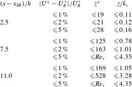
over the remainder of the rough patch, zone R2, are shown in figure 14. Compared to the smooth patch (figure 11) it appears that the profiles are recovered to a higher
 $z^{+}$
after a fetch of
 $11h$
. The recovery over the rough patch is quantified in table 4, which confirms that recovery occurs faster compared to the recovery over the smooth patch (compare table 4 with table 3). Based on the 2 % threshold, recovery in
 $U^{+}$
over the rough patch (versus smooth patch) reaches up to
 $z^{+}\simeq 21$
(versus
 $z^{+}\simeq 6$
) after a fetch of
 $2.5h$
,
 $z^{+}\simeq 475$
(versus
 $z^{+}\simeq 18$
) after a fetch of
 $7.5h$
and
 $z^{+}\simeq 528$
(versus
 $z^{+}\simeq 48$
) after a fetch of
 $11h$
.
Recovery in
 $U^{+}$
of case
 $24h$
after the smooth-to-rough step change based on the 1 %, 2 % or 5 % difference with the
 $U_{R}^{+}$
profile of fully developed homogeneous rough wall open-channel flow. The fully developed case is at
 $Re_{\unicode[STIX]{x1D70F}}=704$
with the same roughness properties and channel height as the smooth-to-rough case. Here
 $k_{s}\approx 30z_{0}\approx 4.1k$
.

The study in this section yields a higher reliability of equilibrium assumptions over the rough patch than the smooth patch. If an error up to 5 % were considered acceptable and if the beginning of the log layer is classically noted as 30 wall units above the wall, over the rough patch the log-law assumption becomes valid (i.e. recovery reaches the beginning of the log layer) after a fetch of
 $2.5h$
. However, over the smooth patch the same assumption is valid only after a fetch of
 $5h$
. This conclusion is consistent with the results of Bou-Zeid et al. (Reference Bou-Zeid, Meneveau and Parlange2005) who compared WMLES of rougher-to-smoother transition (and vice versa) with the field measurements of Bradley (Reference Bradley1968). They observed large discrepancy with the field measurements at the initial
 $5h$
distance after each step change. The discrepancy was decreased by further refining the grid and resolving the flow to a lower
 $z^{+}$
.
3.3 Internal boundary layer
This section studies the IBL and attempts to find a proper definition for its thickness
 $\unicode[STIX]{x1D6FF}_{i}$
. The literature has not converged on a unified definition of
 $\unicode[STIX]{x1D6FF}_{i}$
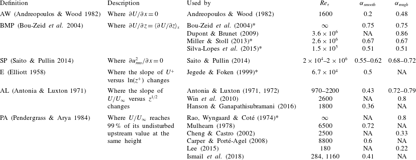
, and this consequently hinders a systematic comparison of the IBL growth rates. To demonstrate this divergence of views, some of the common definitions and the previous studies that have adopted these definitions are outlined in table 5. The corresponding
 $Re_{\unicode[STIX]{x1D70F}}$
in each study as well as the obtained power-law exponents
 $\unicode[STIX]{x1D6FC}$
for the IBL growth rate (
 $\unicode[STIX]{x1D6FF}_{i}\propto x^{\unicode[STIX]{x1D6FC}}$
) are added to the table.
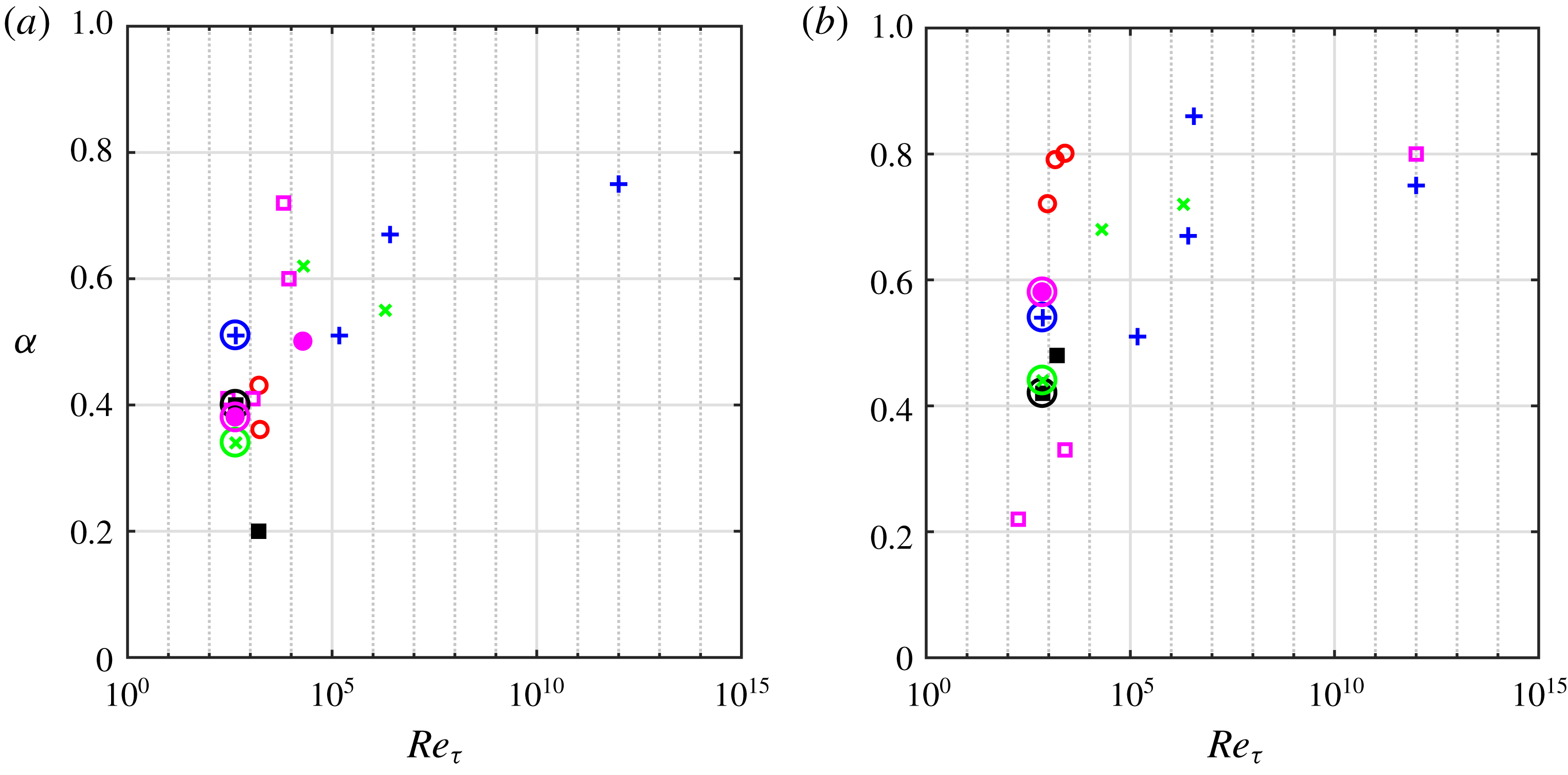
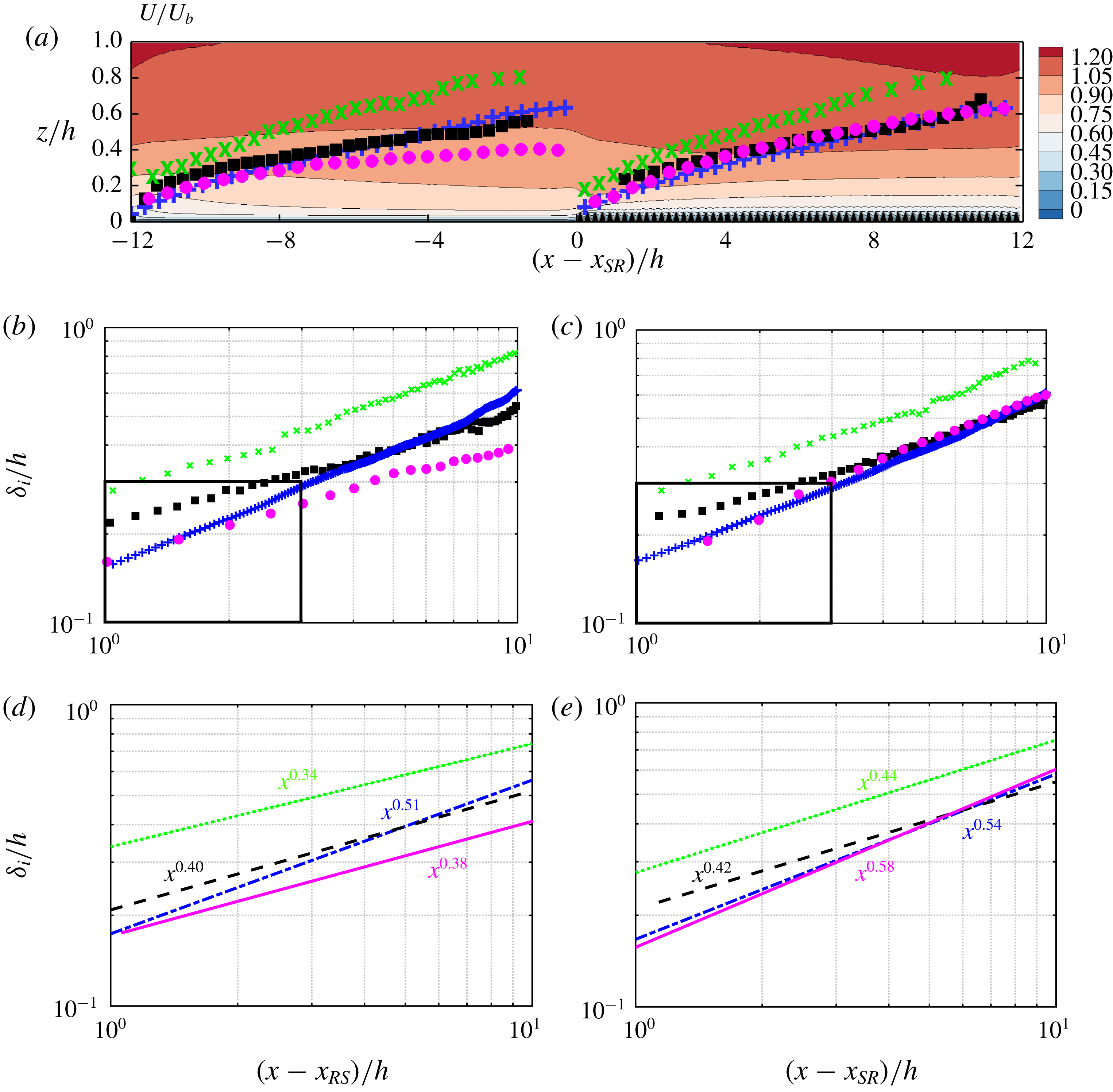
The obtained power-law exponents in table 5 are compiled in figure 15. To ease the interpretation, the studies that have adopted the same definition are shown with the same symbol (and the same colour). Additionally, the results of some of the definitions that were applied to case
 $24h$
are added to figure 15, and are highlighted with circled symbols. At a fixed Reynolds number over either the smooth or the rough patch, the obtained values of
 $\unicode[STIX]{x1D6FC}$
from different definitions are substantially different from each other. This is also supported by the 50 % variance seen in the resulting values of
 $\unicode[STIX]{x1D6FC}$
, obtained from case
 $24h$
. Thus, it appears that part of the scatter seen in figure 15 stems from the different definitions. Note that the studies highlighted with asterisks in table 5 considered transitions from a rougher to a smoother surface. Disregarding these studies from figure 15 (which correspond to some symbols for
 $Re_{\unicode[STIX]{x1D70F}}>6\times 10^{4}$
) does not reduce the scatter caused by the IBL definition. In this section, the definitions of
 $\unicode[STIX]{x1D6FF}_{i}$
arranged in table 5 are discussed further, through their application to case
 $24h$
. Eventually, a reliable definition is proposed according to the physical justifications.
Summary of the definitions of
 $\unicode[STIX]{x1D6FF}_{i}$
commonly used in the literature, and the previous studies that have adopted these definitions. For each study, the corresponding
 $Re_{\unicode[STIX]{x1D70F}}$
, as well as the obtained power-law exponent (
 $\unicode[STIX]{x1D6FC}$
in
 $\unicode[STIX]{x1D6FF}_{i}\propto x^{\unicode[STIX]{x1D6FC}}$
), is reported for rough-to-smooth (
 $\unicode[STIX]{x1D6FC}_{smooth}$
) and smooth-to-rough (
 $\unicode[STIX]{x1D6FC}_{rough}$
) step changes. The studies highlighted by asterisks are numerical simulations which considered transitions from rougher surfaces to smoother surfaces (or vice versa), as imposed by different roughness heights
 $z_{0}$
. Thus,
 $\unicode[STIX]{x1D6FC}_{smooth}$
and
 $\unicode[STIX]{x1D6FC}_{rough}$
for these studies imply the IBL power-law exponents over the smoother surface and rougher surface, respectively.

Values of the power-law exponent
 $\unicode[STIX]{x1D6FC}$
for
 $\unicode[STIX]{x1D6FF}_{i}$
from the previous studies in table 5. Studies that have adopted the same definition of
 $\unicode[STIX]{x1D6FF}_{i}$
are indicated with the same symbol. (a) Rough-to-smooth and (b) smooth-to-rough step change. AW (▪); AL (○); BMP (+); SP (
 $\times$
); E (●); PA (▫). The circled symbols at
 $Re_{\unicode[STIX]{x1D70F}}=443$
(a) and
 $Re_{\unicode[STIX]{x1D70F}}=715$
(b) are obtained from application of different definitions of
 $\unicode[STIX]{x1D6FF}_{i}$
to case
 $24h$
.

Application of the definitions of
 $\unicode[STIX]{x1D6FF}_{i}$
in table 5 to case
 $24h$
. (a) AW, (b) BMP, (c) SP, (d) E, (e) AL. In each panel the contour plot shows the characteristic parameter to identify
 $\unicode[STIX]{x1D6FF}_{i}$
, and the symbols locate
 $\unicode[STIX]{x1D6FF}_{i}$
based on the corresponding definition (
 $\unicode[STIX]{x1D6FF}_{AW}$
(▪),
 $\unicode[STIX]{x1D6FF}_{BMP}$
(+),
 $\unicode[STIX]{x1D6FF}_{SP}$
(
 $\times$
),
 $\unicode[STIX]{x1D6FF}_{E}$
(●)). In (e) detecting
 $\unicode[STIX]{x1D6FF}_{i}$
from AL was not straightforward (refer to text). The fields are overlaid by the spanwise projection of the roughness, in black colour.

Figure 16 shows the application of the definitions of
 $\unicode[STIX]{x1D6FF}_{i}$
(table 5) to case
 $24h$
. Each field in figure 16 shows the characteristic parameter (e.g.
 $\unicode[STIX]{x2202}U/\unicode[STIX]{x2202}x$
,
 $\unicode[STIX]{x2202}u_{rms}/\unicode[STIX]{x2202}x$
) to quantify
 $\unicode[STIX]{x1D6FF}_{i}$
based on each definition. All the definitions are invariant to the normalising velocity or length scale. The markers on each panel locate
 $\unicode[STIX]{x1D6FF}_{i}$
based on the corresponding definition. However, for definition AL (figure 16
e) it is not trivial to identify
 $\unicode[STIX]{x1D6FF}_{i}$
from the current data. To recognise the different definitions, the subscript of
 $\unicode[STIX]{x1D6FF}_{i}$
shows the definition used from table 5 (e.g.
 $\unicode[STIX]{x1D6FF}_{BMP}$
is obtained from BMP, Bou-Zeid et al.
Reference Bou-Zeid, Meneveau and Parlange2004).
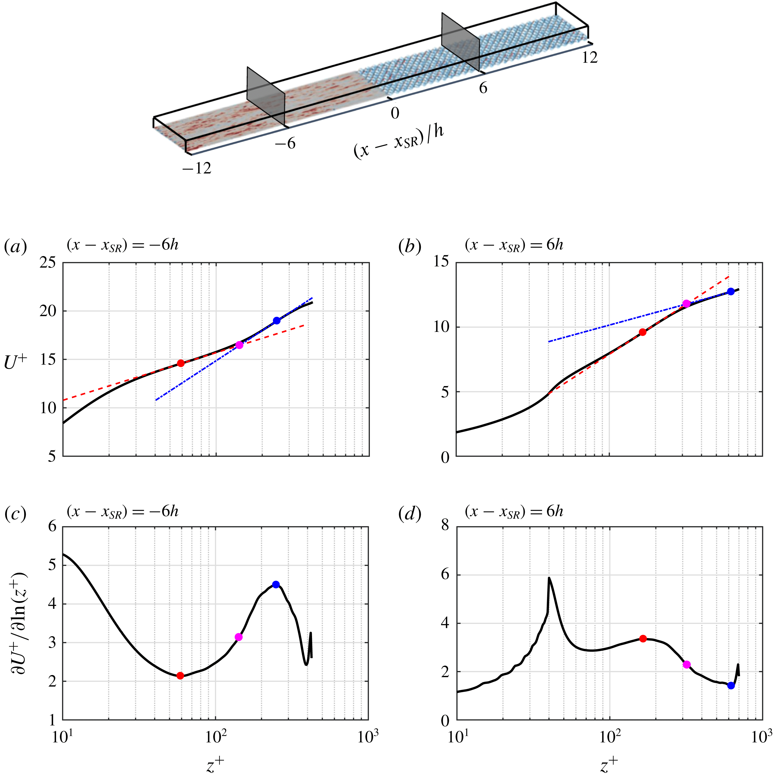
Identifying
 $\unicode[STIX]{x1D6FF}_{E}$
from logarithmic slope change. The quantities are normalised by the local
 $u_{\unicode[STIX]{x1D70F}}$
and
 $\unicode[STIX]{x1D708}$
. Profiles of (a,b)
 $U^{+}$
at
 $(x-x_{SR})=-6h$
and
 $6h$
, indicated in the computational domain. Profiles of (c,d)
 $\unicode[STIX]{x2202}U^{+}/\unicode[STIX]{x2202}\ln (z^{+})$
corresponding to the profiles in (a,b). The inner and outer slopes are the extrema of
 $\unicode[STIX]{x2202}U^{+}/\unicode[STIX]{x2202}\ln (z^{+})$
(●, red; ●, blue). Here
 $\unicode[STIX]{x1D6FF}_{E}$
(●, magenta) is located by intersecting the inner (– – –) and outer (– - – - –) logarithmic fitting lines.

Figure 16(a) corresponds to
 $\unicode[STIX]{x1D6FF}_{AW}$
based on
 $\unicode[STIX]{x2202}U/\unicode[STIX]{x2202}x$
. As was discussed in § 3.2,
 $\unicode[STIX]{x2202}U/\unicode[STIX]{x2202}x$
is a measure of flow acceleration/deceleration. Originally this method was applied to boundary layer data, and a threshold was necessary for
 $\unicode[STIX]{x2202}U/\unicode[STIX]{x2202}x\simeq 0$
. This is due to the unbounded nature of the boundary layer, in which the flow acceleration/deceleration near the wall is gradually decreased to zero away from the wall (Hanson & Ganapathisubramani Reference Hanson and Ganapathisubramani2016). For the channel flow, since
 $\unicode[STIX]{x2202}U/\unicode[STIX]{x2202}x$
changes its sign at some distance away from the wall (§ 3.2), detecting
 $\unicode[STIX]{x2202}U/\unicode[STIX]{x2202}x=0$
is straightforward. Figure 16(b,c) corresponds to
 $\unicode[STIX]{x1D6FF}_{BMP}$
and
 $\unicode[STIX]{x1D6FF}_{SP}$
, respectively. Parameter
 $\unicode[STIX]{x1D6FF}_{BMP}$
is defined as the height where the local
 $\unicode[STIX]{x2202}U/\unicode[STIX]{x2202}z$
is equal to its
 $x$
-averaged value,
 $\langle .\rangle _{x}$
, and
 $\unicode[STIX]{x1D6FF}_{SP}$
is based on
 $\unicode[STIX]{x2202}u_{rms}^{2}/\unicode[STIX]{x2202}x=0$
.
Figure 16(d) shows the characterising parameter to identify
 $\unicode[STIX]{x1D6FF}_{E}$
, defined based on the observation made in § 3.2. The mean velocity profile after a surface change yields two logarithmic slopes. The inner slope is the result of the new surface and the outer slope is the imprint of the previous surface. Elliott (Reference Elliott1958) defines
 $\unicode[STIX]{x1D6FF}_{E}$
as the intersection point of inner and outer slopes. To detect the slopes in each
 $x$
-location, the slope curve
 $\unicode[STIX]{x2202}U^{+}/\unicode[STIX]{x2202}\ln (z^{+})$
is plotted for the velocity profile at that location. This is demonstrated in figure 17 for a profile in the middle of the smooth patch (figure 17
a,c) and for a profile in the middle of the rough patch (figure 17
b,d). Note that the choice for scaling the profiles (here
 $u_{\unicode[STIX]{x1D70F}}$
and
 $\unicode[STIX]{x1D708}$
) does not affect the obtained
 $\unicode[STIX]{x1D6FF}_{E}$
. The inner and outer logarithmic slopes appear as extrema in
 $\unicode[STIX]{x2202}U^{+}/\unicode[STIX]{x2202}\ln (z^{+})$
. Once the slopes (extrema) are found, two fitting lines with the same slopes are passed through the velocity profile at the located extrema. Here
 $\unicode[STIX]{x1D6FF}_{E}$
is identified by intersecting the two fitted lines. Application of this approach to the whole field is shown in figure 16(d). The inner and outer slopes can be recognised as the two distinct (blue and red) regions. In addition to Elliott (Reference Elliott1958), Panofsky & Townsend (Reference Panofsky and Townsend1964) proposed a variant of
 $\unicode[STIX]{x1D6FF}_{E}$
where
 $\unicode[STIX]{x1D6FF}_{i}$
was placed higher up, at the beginning of the upper logarithmic region. Here, the definition by Elliott (Reference Elliott1958) is preferred as Panofsky & Townsend’s (Reference Panofsky and Townsend1964) definition requires a threshold for the upper logarithmic region, while Elliott’s (Reference Elliott1958) definition, based on the intersection of the two logarithmic lines, is not dependent on a threshold.
The same slope-based approach was followed to calculate
 $\unicode[STIX]{x1D6FF}_{AL}$
(Antonia & Luxton Reference Antonia and Luxton1971). According to this definition, if the mean velocity is plotted against
 $z^{1/2}$
, it yields two distinct straight-line slopes and
 $\unicode[STIX]{x1D6FF}_{AL}$
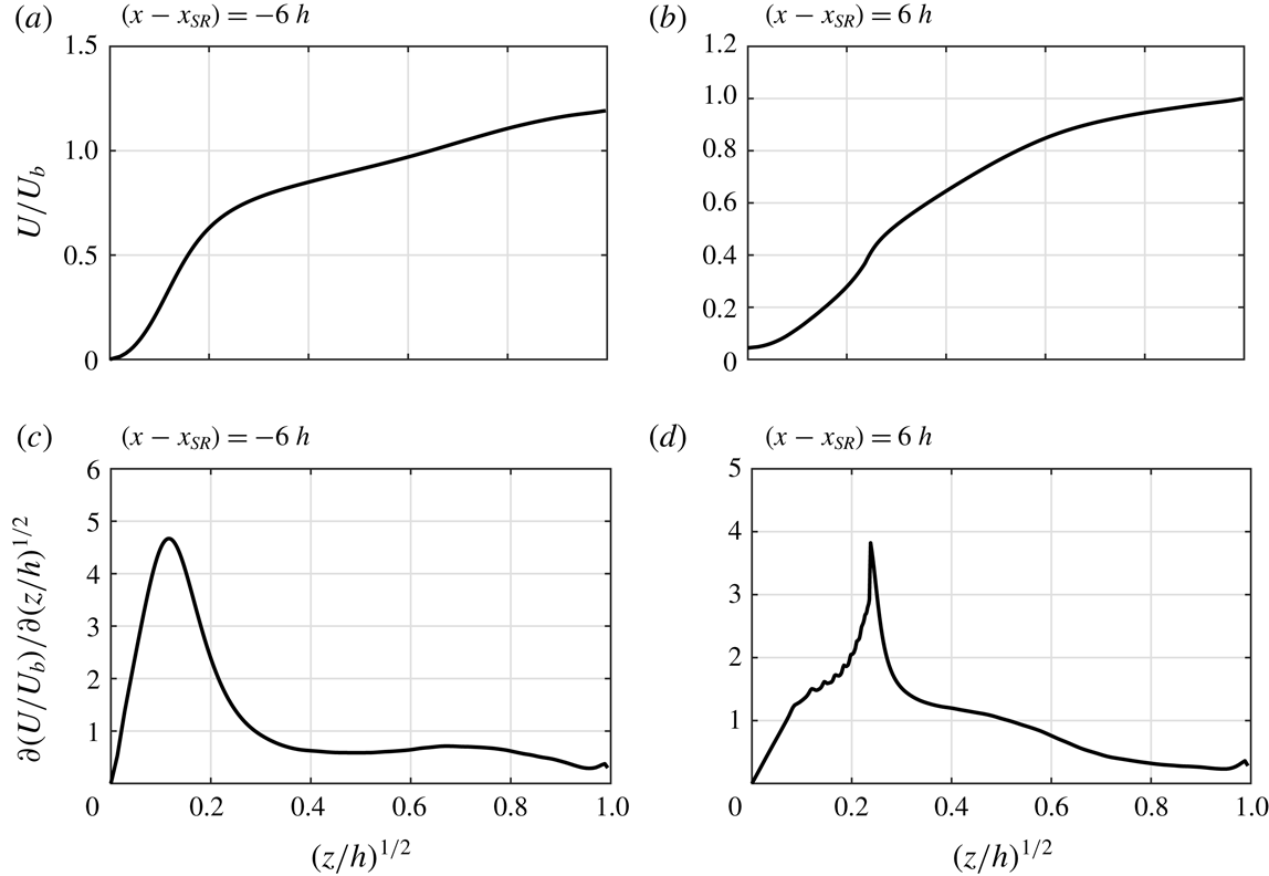
falls at their intersection. The profiles of
 $U/U_{b}$
versus
 $(z/h)^{1/2}$
, over both the smooth and rough patches, are shown in figure 18. The profiles do not show two slopes. This is supported by the slope curves
 $\unicode[STIX]{x2202}(U/U_{b})/\unicode[STIX]{x2202}(z/h)^{1/2}$
(figure 18
c,d). Other than distinct peaks close to the wall, there are no clear extrema and no signs of the two distinct slopes that should be yielded by this technique. Figure 16(e) shows the characteristic parameter
 $\unicode[STIX]{x2202}(U/U_{b})/\unicode[STIX]{x2202}(z/h)^{1/2}$
over the entire domain. Due to the gradual variation of this quantity,
 $\unicode[STIX]{x1D6FF}_{AL}$
is difficult to detect. The problem in applying this technique may lie with the lower Reynolds number of the current simulation. The experiments where this technique was applied extended up to and beyond
 $Re_{\unicode[STIX]{x1D70F}}\simeq 2000$
.
The method proposed by Pendergrass & Arya (Reference Pendergrass and Arya1984) is not applicable to channel flow as is quantified based on the velocity deviation from its undisturbed profile upstream of the surface change. In a channel flow there is a strong acceleration/deceleration during each surface change (figure 7
b) that substantially modifies the
 $U$
profile across the entire channel. Hence the new profile is no longer comparable to the one upstream.
Profiles of (a,b)
 $U/U_{b}$
versus
 $(z/h)^{1/2}$
at the same locations indicated in figure 17. Profiles of (c,d) the slope curves,
 $\unicode[STIX]{x2202}(U/U_{b})/\unicode[STIX]{x2202}(z/h)^{1/2}$
, corresponding to the profiles in (a,b).

Comparison between the definitions of
 $\unicode[STIX]{x1D6FF}_{i}$
throughout the domain in linear scale (a). The resulting
 $\unicode[STIX]{x1D6FF}_{i}$
plotted in log scale over (b) the smooth patch and (c) the rough patch. Note that the origin has been shifted to the beginning of the smooth patch (
 $x_{RS}$
) in (b,d). Power-law fitting the resulting
 $\unicode[STIX]{x1D6FF}_{i}$
over (d) the smooth patch and (e) the rough patch. Definitions:
 $\unicode[STIX]{x1D6FF}_{AW}$
(▪, – – –);
 $\unicode[STIX]{x1D6FF}_{BMP}$
(+, – - – - –);
 $\unicode[STIX]{x1D6FF}_{SP}$
(
 $\times$
,
- - - -);
 $\unicode[STIX]{x1D6FF}_{E}$
(●, ——). The framed regions in (b,c) highlight the close behaviour of
 $\unicode[STIX]{x1D6FF}_{E}$
and
 $\unicode[STIX]{x1D6FF}_{BMP}$
within a fetch of
 $3h$
.

All
 $\unicode[STIX]{x1D6FF}_{i}$
values calculated from the different definitions are plotted in figure 19. Over the rough patch (figure 19
c,e), with the exception of
 $\unicode[STIX]{x1D6FF}_{SP}$
(
 $\times$
), the three other definitions yield almost identical growth rates, especially for
 $(x-x_{SR})\geqslant 4h$
. However, over the smooth patch, a discrepancy of up to 100 % is seen among the definitions. Assessment of the obtained values of
 $\unicode[STIX]{x1D6FC}$
(figure 19
d,e) reveals their sensitivity to definition, which was earlier conjectured as one possible cause of scatter in the literature (figure 15). One notable behaviour in
 $\unicode[STIX]{x1D6FF}_{BMP}$
(+) is its almost identical growth rate over the smooth and rough patches, an observation that was earlier discussed by Bou-Zeid et al. (Reference Bou-Zeid, Meneveau and Parlange2004) and Silva-Lopes et al. (Reference Silva-Lopes, Palma and Piomelli2015). Both Bou-Zeid et al. (Reference Bou-Zeid, Meneveau and Parlange2004) and Silva-Lopes et al. (Reference Silva-Lopes, Palma and Piomelli2015) considered transitions from a rougher surface to a smoother surface (and vice versa), with roughness height ratios of
 $z_{01}/z_{02}=10^{-1}$
and
 $z_{01}/z_{02}\approx 10^{-3}$
, respectively. Despite the differences between the current DNS and these two studies, in each study
 $\unicode[STIX]{x1D6FF}_{BMP}$
yields the same power-law scaling over both smooth (or smoother) and rough (or rougher) surfaces, albeit with different power-law scaling
 $\unicode[STIX]{x1D6FC}$
between the studies.
One key finding from this section is the sensitivity of
 $\unicode[STIX]{x1D6FF}_{i}$
to its definition. This explains some of the discrepancies in the literature. The remainder of this section attempts to arrive at a physically motivated definition. The IBL definition must be consistent with the IBL concept, a layer that is influenced by the new surface and above which the flow does not feel the surface underneath. This concept also includes turbulence characteristics, i.e. turbulence characteristics within the IBL differ from those above. However, all the definitions of
 $\unicode[STIX]{x1D6FF}_{i}$
in table 5 (except
 $\unicode[STIX]{x1D6FF}_{SP}$
) are derived from the mean velocity. Therefore, a fair examination of consistency between the IBL concept and the IBL definitions would be through the turbulence characteristics.
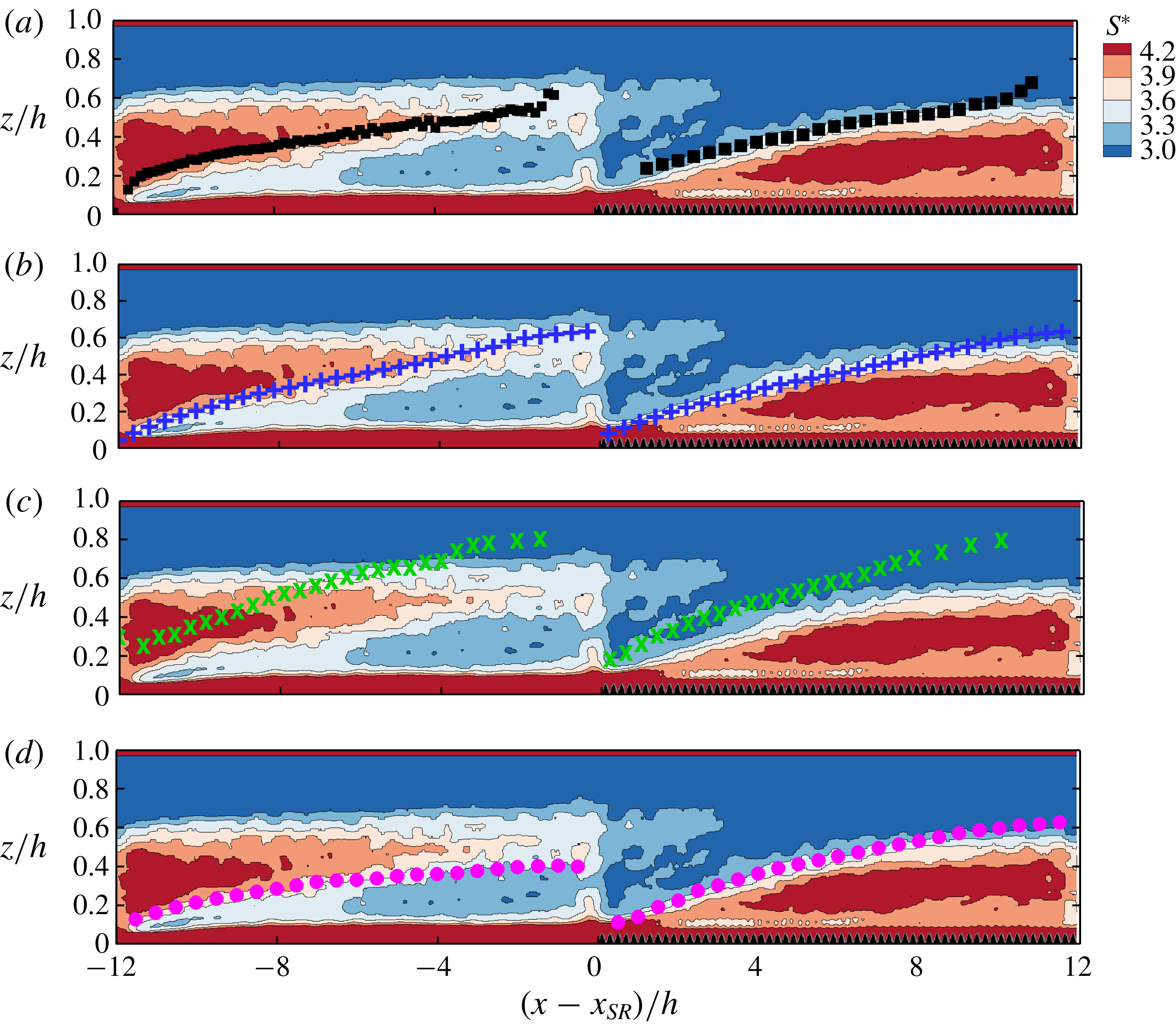
The normalised mean shear rate
 $S^{\ast }=|S|{\mathcal{K}}/\unicode[STIX]{x1D700}$
, overlaid with the IBL definitions: (a)
 $\unicode[STIX]{x1D6FF}_{AW}$
(▪), (b)
 $\unicode[STIX]{x1D6FF}_{BMP}$
(+), (c)
 $\unicode[STIX]{x1D6FF}_{SP}$
(
 $\times$
) and (d)
 $\unicode[STIX]{x1D6FF}_{E}$
(●). The fields are overlaid by the spanwise projection of the roughness, in black colour.

Various definitions may be chosen to characterise turbulence. Here, the ratio of the turbulent time scale over the mean time scale
 $S^{\ast }\equiv |S|{\mathcal{K}}/\unicode[STIX]{x1D700}$
(Pope Reference Pope2000, § 7.1.7) is selected, where
 ${\mathcal{K}}$
and
 $\unicode[STIX]{x1D700}$
are the turbulent kinetic energy and its dissipation rate, respectively. Parameter
 $|S|=\sqrt{2S_{ij}S_{ij}}$
is the mean strain-rate magnitude. In an equilibrium smooth-channel flow at
 $Re_{\unicode[STIX]{x1D70F}}\simeq 395$
,
 $S^{\ast }$
is almost constant for
 $0.1\leqslant z/h\leqslant 0.7$
(less than
 $\pm 10\,\%$
variation). This range covers the heights above the buffer region up to the outer wake region. The constant
 $S^{\ast }$
is linked to the production–dissipation balance and constancy of the normalised Reynolds shear stress by
 ${\mathcal{K}}$
(Pope Reference Pope2000). In figure 20,
 $S^{\ast }$
is plotted, overlaid by the four IBL definitions. The region very close to the bottom surface (the red region for
 $z/h\lesssim 0.1$
) corresponds to the viscous and buffer regions, and is disregarded. Considering
 $0.1\leqslant z/h\leqslant 0.6$
,
 $S^{\ast }$
highlights two distinct regions, which differ in turbulence characteristics. The region closer to the wall is influenced by the new surface, while the region away from the wall preserves the characteristics associated with the previous surface. Among all the IBL definitions,
 $\unicode[STIX]{x1D6FF}_{E}$
appears to behave more consistently with the distinct regions created by
 $S^{\ast }$
. Over the rough patch, all the IBL definitions, except
 $\unicode[STIX]{x1D6FF}_{SP}$
, behave in a manner consistent with the distinct regions. However, over the smooth patch, only
 $\unicode[STIX]{x1D6FF}_{E}$
captures the sharp gradient in
 $S^{\ast }$
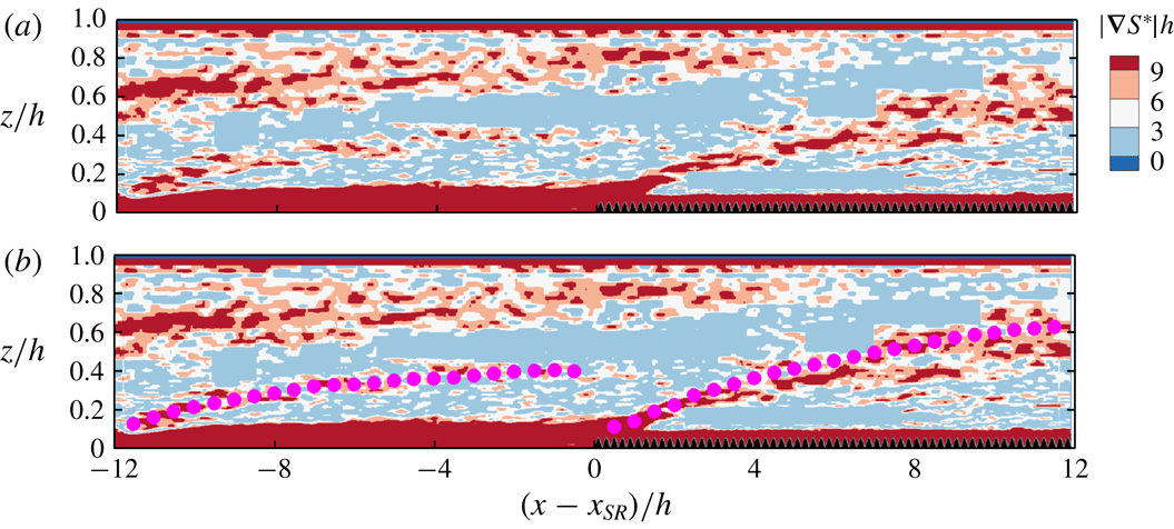
that marks the edge of the IBL. As a support to the latter argument, the gradient magnitude of
 $S^{\ast }$
,
 $|\unicode[STIX]{x1D735}S^{\ast }|=\sqrt{(\unicode[STIX]{x2202}S^{\ast }/\unicode[STIX]{x2202}x)^{2}+(\unicode[STIX]{x2202}S^{\ast }/\unicode[STIX]{x2202}z)^{2}}$
, is plotted in figure 21. The regions where this quantity is maximum correspond to the regions where
 $S^{\ast }$
has the largest variation (i.e. turbulence characteristics are changing). As is seen in figure 21(a), the regions of maximum
 $|\unicode[STIX]{x1D735}S^{\ast }|$
appear as layers that are emanated from the leading edges of the smooth and rough patches. In figure 21(b) it is seen that over each patch,
 $\unicode[STIX]{x1D6FF}_{E}$
is coincident with this newly formed layer of maximum
 $|\unicode[STIX]{x1D735}S^{\ast }|$
that is emanated from the leading edge of each patch.
The gradient magnitude of
 $S^{\ast }$
(
 $|\unicode[STIX]{x1D735}S^{\ast }|$
) corresponding to figure 20 is shown in (a) and (b). In (b)
 $|\unicode[STIX]{x1D735}S^{\ast }|$
is overlaid with
 $\unicode[STIX]{x1D6FF}_{E}$
(●). The fields are overlaid by the spanwise projection of the roughness, in black colour.

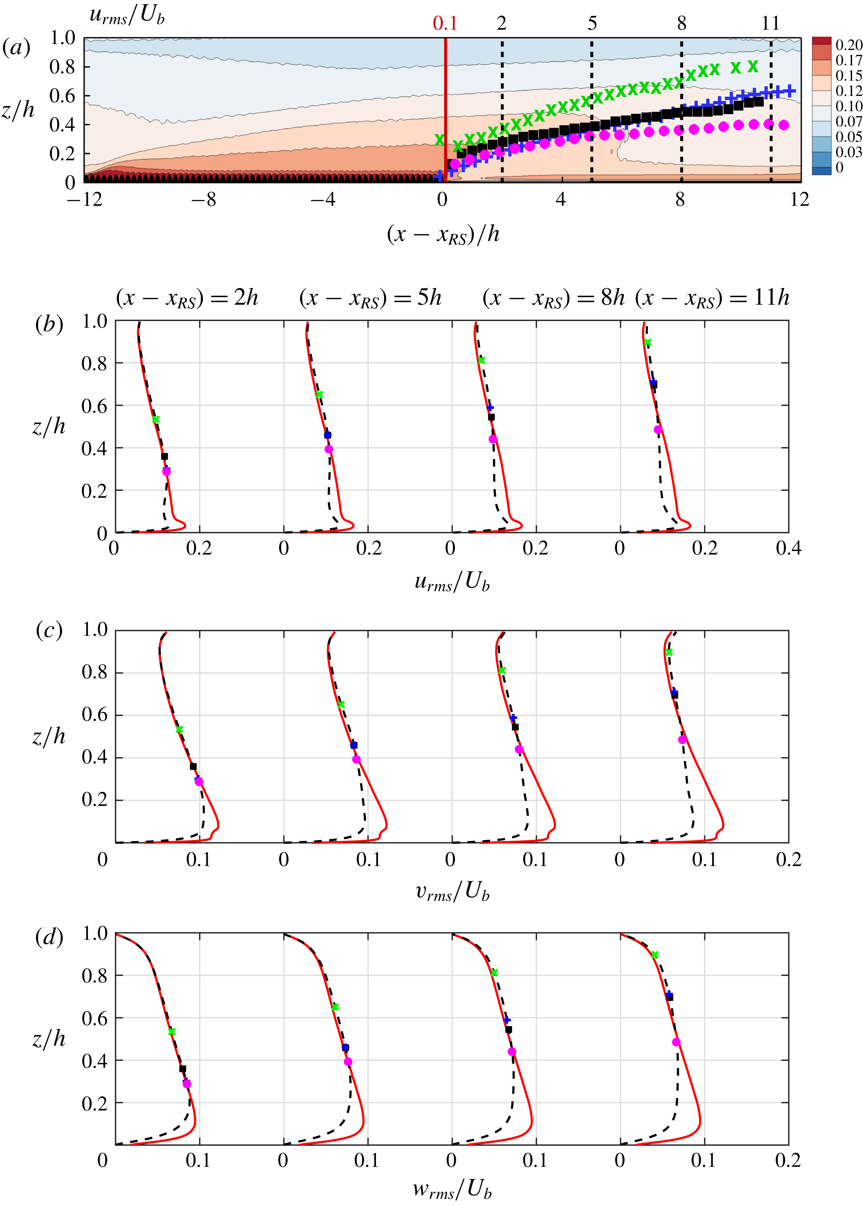
(a) The
 $u_{rms}$
field overlaid with the IBL definitions. Comparison of profiles of (b)
 $u_{rms}$
, (c)
 $v_{rms}$
and (d)
 $w_{rms}$
, after a fetch of
 $2h$
,
 $5h$
,
 $8h$
and
 $11h$
over the smooth patch (– – –), with their upstream counterparts after a fetch of
 $0.1h$
(——). The extracted locations are indicated in the
 $u_{rms}$
field in (a). The four overlaid IBL definitions are:
 $\unicode[STIX]{x1D6FF}_{AW}$
(▪),
 $\unicode[STIX]{x1D6FF}_{BMP}$
(+),
 $\unicode[STIX]{x1D6FF}_{SP}$
(
 $\times$
) and
 $\unicode[STIX]{x1D6FF}_{E}$
(●). The spanwise projection of the ‘egg-carton’ roughness is indicated with black colour.

Consistency of the IBL definitions with the IBL concept is examined through the r.m.s. quantities over the smooth patch in figure 22. Profiles of
 $u_{rms}$
(figure 22
b),
 $v_{rms}$
(figure 22
c) and
 $w_{rms}$
(figure 22
d), at a fetch of
 $2h,5h,8h$
and
 $11h$
over the smooth patch (– – –) are compared with their upstream counterparts immediately downstream of the rough-to-smooth step change, at a fetch of
 $0.1h$
(——). At each downstream location, the height up to which the r.m.s. profile departs from its upstream counterpart indicates the maximum height to which the new surface influence has reached (i.e. IBL concept based on r.m.s. quantities). Figure 22 shows that among the four overlaid
 $\unicode[STIX]{x1D6FF}_{i}$
definitions,
 $\unicode[STIX]{x1D6FF}_{E}$
(●) coincides better with the departure point for all three r.m.s. quantities; this is more evident in the most downstream profile at
 $(x-x_{RS})=11h$
. The same study was conducted over the rough patch (not shown), and with the exception of
 $\unicode[STIX]{x1D6FF}_{SP}$
the three other definitions agreed well with the departure point. Therefore, from turbulence characteristics and r.m.s. quantities it is concluded that
 $\unicode[STIX]{x1D6FF}_{E}$
is more consistent with the IBL concept. Based on either turbulence characteristics
 $S^{\ast }$
(figures 20 and 21) or any of the r.m.s. quantities (figure 22), Elliott’s (Reference Elliott1958) definition (
 $\unicode[STIX]{x1D6FF}_{E}$
, ●) is consistent with the IBL concept. Therefore, any new IBL definition that is derived from
 $S^{\ast }$
or Reynolds stresses would be no different from
 $\unicode[STIX]{x1D6FF}_{E}$
.
This section represents the first to analyse the IBL definitions so extensively, highlighting the large discrepancy in IBL growth rates from the various definitions for the same flow. We can thus propose the most physically consistent IBL definition.
4 Conclusions
In this study, DNS of open-channel flow over streamwise-alternating patches of smooth and fully rough walls were investigated. The computational domain was equally divided between the smooth patch and the rough patch. Owing to the streamwise periodicity, both rough-to-smooth and smooth-to-rough step changes were studied. With the detailed information provided by DNS, some aspects of this flow were investigated that were hard to explore through either experimental techniques or computational models. These aspects included: (1) the validity of the equilibrium assumptions and (2) a thorough study of the IBL definitions.
Before studying the above-mentioned aspects, it was ensured that the parameters of interest are invariant to the finite domain size, and its periodicity. For this aim, three cases with domain lengths varying from 6 to 24 times the channel height
 $h$
as well as a non-periodic rough-to-smooth case with fully developed inflow were simulated. The results showed that with a domain length of at least
 $12h$
(assigning
 $6h$
to each patch), the flow quantities within the IBL are not influenced by the domain length and periodicity. Above the IBL, due to the history effects, the flow remains sensitive. Nevertheless, the physics of interest occur within the IBL or at its edge, including the wall shear stress, the IBL thickness and the flow recovery.
Assessment of the mean velocity profiles revealed that the equilibrium assumptions are not entirely valid, in particular over the smooth patch. If an error of up to 5 % is noted acceptable and if the beginning of the log layer is classically noted as 30 wall units above the wall, over the rough patch the log-law assumption becomes valid after a fetch of
 $2.5h$
, while over the smooth patch it is valid after a fetch of
 $5h$
.
An extensive study was conducted of the IBL. Most commonly used definitions of the IBL thickness were tested with the current DNS. It was noticed that for the same dataset, depending on the definition, the resulting IBL thickness may differ by up to 100 %. To choose the proper definition, the authors started from the fundamental perception of the IBL, as a layer that separates the region influenced by the surface underneath from the uninfluenced one. Then, they applied this concept to the turbulence characteristics and r.m.s. quantities. Results showed that the definition by Elliott (Reference Elliott1958), which is based on the logarithmic slope change of the velocity profile, is more consistent with this perception of the IBL.
Acknowledgements
This research was supported by resources provided by the Pawsey Supercomputing Centre with funding from the Australian Government and the Government of Western Australia and by the National Computing Infrastructure (NCI), which is supported by the Australian Government. This research was partially supported under the Australian Research Councils Discovery Projects funding scheme (project DP160103619). The authors acknowledge the helpful comments by Professor E. Bou-Zeid and the two other anonymous referees.
Appendix A. Numerical scheme and the IBM
In this appendix details of the numerical scheme, the IBM and verification of the numerical set-up against a body-conforming grid solver are presented.
Equation (2.1) in § 2 is integrated in time using the fractional-step algorithm (Perot Reference Perot1993). The time-marching scheme is the third-order Runge–Kutta (Spalart et al.
Reference Spalart, Moser and Rogers1991), which divides each time step into three sub-steps. During each sub-step, the fractional-step algorithm consists of the following three steps to update the velocity from the current sub-step (
 $u_{i}^{n}$
) to the next sub-step (
 $u_{i}^{n+1}$
).
(1) Predicting the intermediate velocity (
 $u_{i}^{\ast }$
): (A 1)$$\begin{eqnarray}\displaystyle & \displaystyle \frac{u_{i}^{\ast }-u_{i}^{n}}{\unicode[STIX]{x1D6E5}_{t}}=\text{Explicit}+\unicode[STIX]{x1D708}\left(\frac{\unicode[STIX]{x2202}^{2}u_{i}}{\unicode[STIX]{x2202}x_{3}^{2}}\right)^{n,\ast }+F_{i}^{m}, & \displaystyle\end{eqnarray}$$
(A 2)$$\begin{eqnarray}\displaystyle & \!\!\displaystyle \text{Explicit}=\unicode[STIX]{x1D709}_{m}\left[-\frac{1}{\unicode[STIX]{x1D70C}}\left\langle \frac{\text{d}P}{\text{d}x}\right\rangle \unicode[STIX]{x1D719}_{u}\unicode[STIX]{x1D6FF}_{i1}-\frac{1}{\unicode[STIX]{x1D70C}}\left(\frac{\unicode[STIX]{x2202}\widetilde{p}}{\unicode[STIX]{x2202}x_{i}}\right)^{\!n}\right]\!+\left[\unicode[STIX]{x1D708}\!\left(\frac{\unicode[STIX]{x2202}^{2}}{\unicode[STIX]{x2202}x_{1}^{2}}+\frac{\unicode[STIX]{x2202}^{2}}{\unicode[STIX]{x2202}x_{2}^{2}}\right)u_{i}-\frac{\unicode[STIX]{x2202}u_{i}u_{j}}{\unicode[STIX]{x2202}x_{j}}\right]^{n,n-1}\!\!. & \displaystyle \nonumber\\ \displaystyle & & \displaystyle\end{eqnarray}$$
(2) Solving the Poisson equation:
(A 3)$$\begin{eqnarray}\frac{1}{\unicode[STIX]{x1D70C}}\frac{\unicode[STIX]{x2202}^{2}[\unicode[STIX]{x1D6FF}\widetilde{p}]}{\unicode[STIX]{x2202}x_{j}^{2}}=\frac{1}{\unicode[STIX]{x1D709}_{m}\unicode[STIX]{x1D6E5}_{t}}\frac{\unicode[STIX]{x2202}u_{i}^{\ast }}{\unicode[STIX]{x2202}x_{i}}.\end{eqnarray}$$
(3) Updating the velocity (
$u_{i}^{n+1}$
) and periodic pressure (
$\widetilde{p}^{n+1}$
) for the next sub-step: (A 4a,b )$$\begin{eqnarray}u_{i}^{n+1}=u_{i}^{\ast }-\frac{\unicode[STIX]{x1D709}_{m}\unicode[STIX]{x1D6E5}_{t}}{\unicode[STIX]{x1D70C}}\frac{\unicode[STIX]{x2202}[\unicode[STIX]{x1D6FF}\widetilde{p}]}{\unicode[STIX]{x2202}x_{i}},\quad \widetilde{p}^{n+1}=\widetilde{p}^{n}+\unicode[STIX]{x1D719}_{p}[\unicode[STIX]{x1D6FF}\widetilde{p}].\end{eqnarray}$$


The spatial discretisation is the fully conservative fourth-order, staggered, finite-difference scheme (Morinishi et al.
Reference Morinishi, Lund, Vasilyev and Moin1998; Verstappen & Veldman Reference Verstappen and Veldman2003). Parameter
 $\unicode[STIX]{x1D709}_{m}\unicode[STIX]{x1D6E5}_{t}$
is one sub-step size, i.e.
 $\unicode[STIX]{x1D6E5}_{t}=\unicode[STIX]{x1D709}_{1}\unicode[STIX]{x1D6E5}_{t}+\unicode[STIX]{x1D709}_{2}\unicode[STIX]{x1D6E5}_{t}+\unicode[STIX]{x1D709}_{3}\unicode[STIX]{x1D6E5}_{t}$
. The advection and the wall-parallel diffusion terms are advanced explicitly using the low-storage third-order Runge–Kutta,
 $(.)^{n,n-1}=\unicode[STIX]{x1D6FE}_{m}(.)^{n}+\unicode[STIX]{x1D701}_{m}(.)^{n-1}$
, while the wall-normal diffusion term is advanced implicitly,
 $(.)^{n,\ast }=\unicode[STIX]{x1D6FC}_{m}(.)^{n}+\unicode[STIX]{x1D6FD}_{m}(.)^{\ast }$
, where
 $\unicode[STIX]{x1D6FC}_{m},\unicode[STIX]{x1D6FD}_{m},\unicode[STIX]{x1D6FE}_{m}$
and
 $\unicode[STIX]{x1D701}_{m}$
depend on the sub-step (Spalart et al.
Reference Spalart, Moser and Rogers1991, its appendix).
To impose the no-slip condition on the bottom smooth and rough surfaces, the IBM force
 $$\begin{eqnarray}F_{i}^{m}=-(1-\unicode[STIX]{x1D719}_{i})[\text{Explicit}+\unicode[STIX]{x1D708}(\unicode[STIX]{x2202}^{2}u_{i}/\unicode[STIX]{x2202}x_{3}^{2})^{n,\ast }+u_{i}^{n}/\unicode[STIX]{x1D6E5}_{t}]\end{eqnarray}$$
is added such that
 $u_{i}^{\ast }=0$
when
 $\unicode[STIX]{x1D719}_{i}=0$
, as written in (A 1). Here
 $\unicode[STIX]{x1D719}_{i}$
is the fraction of each computational cell occupied by the fluid, computed during pre-processing for the staggered velocity components and pressure (
 $\unicode[STIX]{x1D719}_{u},\unicode[STIX]{x1D719}_{v}$
 $\unicode[STIX]{x1D719}_{w}$
and
 $\unicode[STIX]{x1D719}_{p}$
). Through substitution for
 $F_{i}^{m}$
in (A 1), step (1) can be recast into the following equation:
 $$\begin{eqnarray}\left(1-\unicode[STIX]{x1D708}\unicode[STIX]{x1D719}_{i}\unicode[STIX]{x1D6FD}_{m}\unicode[STIX]{x1D6E5}_{t}\frac{\unicode[STIX]{x2202}^{2}}{\unicode[STIX]{x2202}x_{3}^{2}}\right)u_{i}^{\ast }=\unicode[STIX]{x1D719}_{i}\left(1+\unicode[STIX]{x1D708}\unicode[STIX]{x1D6FC}_{m}\unicode[STIX]{x1D6E5}_{t}\frac{\unicode[STIX]{x2202}^{2}}{\unicode[STIX]{x2202}x_{3}^{2}}\right)u_{i}^{n}+\unicode[STIX]{x1D6E5}_{t}\unicode[STIX]{x1D719}_{i}\,\text{Explicit}.\end{eqnarray}$$
The term in the brackets on the left-hand side of (A 6) is a heptadiagonal matrix (owing to the fourth-order discretisation), which is solved directly for
 $u_{i}^{\ast }$
.
The wall shear stress at each time step at each
 $(x,y)$
location can be obtained through integration of the streamwise IBM force term
 $F_{1}^{m}$
over the
 $z$
-direction:
 $$\begin{eqnarray}\frac{\unicode[STIX]{x1D70F}_{w}}{\unicode[STIX]{x1D70C}}=-\mathop{\sum }_{m=1}^{3}\left[\int _{z_{min}}^{z_{max}}F_{1}^{m}\,\text{d}z\right],\end{eqnarray}$$
where the integrals are summed over the three sub-steps of Runge–Kutta (i.e.
 $m=1,2,3$
), and
 $z_{min}$
and
 $z_{max}$
are the minimum and maximum
 $z$
-coordinates of the computational domain (here
 $-4/3k$
and
 $h$
, respectively). The friction velocity
 $u_{\unicode[STIX]{x1D70F}}(x)=\sqrt{\langle \unicode[STIX]{x1D70F}_{w}\rangle /\unicode[STIX]{x1D70C}}$
is obtained through averaging
 $\unicode[STIX]{x1D70F}_{w}$
over time and spanwise direction. Over the rough patch
 $\langle .\rangle$
also indicates averaging over a finite streamwise window size, following the procedure described in § 2.
This IBM is of the direct-forcing category with the volume of fluid interpolation (Fadlun et al.
Reference Fadlun, Verzicco, Orlandi and Mohd-Yusof2000) suitable for implementing solid geometries in Cartesian codes. In this method the computational domain includes both the solid and fluid regions (figure 2
a), from
 $z_{min}=(-4/3)k$
to
 $z_{max}=h$
, placing a
 $(1/3)k$
solid gap between the roughness trough and the bottom computational boundary, with the no-slip condition imposed on the bottom boundary. To drive only the fluid zone,
 $\langle \text{d}P/\text{d}x\rangle$
has been multiplied by
 $\unicode[STIX]{x1D719}_{u}$
in (A 1). The direct-forcing IBM with the volume of fluid interpolation has been adopted in previous rough-wall simulations (Scotti Reference Scotti2006; Yuan & Piomelli Reference Yuan and Piomelli2014). However, the IBM adopted here has been slightly modified compared to the one adopted by Scotti (Reference Scotti2006) and Yuan & Piomelli (Reference Yuan and Piomelli2014) by adding (A 4b
) in step (3), which corrects the pressure by
 $\unicode[STIX]{x1D719}_{p}$
. With this modification,
 $F_{i}^{m}$
is non-zero only in the computational cells that intersect the solid–fluid interface. However, in the uncorrected approach
 $F_{i}^{m}$
is also non-zero in the non-intersecting in-solid cells. The modified approach yields
 $u_{\unicode[STIX]{x1D70F}}$
more directly in heterogeneous flows.
Comparison between cases
 $6h$
(——) and
 $6h$
verification (○). (a) Reynolds number
 $Re_{\unicode[STIX]{x1D70F}}$
based on local
 $u_{\unicode[STIX]{x1D70F}}$
and
 $h$
. Profiles of (b)
 $U$
and (c)
 $u_{rms}$
. The quantities in plus units are normalised by the local
 $u_{\unicode[STIX]{x1D70F}}$
and
 $\unicode[STIX]{x1D708}$
. Comparison is made in the middle of the smooth patch (lower curves in b,c) and in the middle of the rough patch (upper curves in b,c), demonstrated in the domains on the right-hand side.

Summary of the verification case using the body-conforming grid solver (Cascade Technologies, Inc.; Ham, Mattsson & Iaccarino Reference Ham, Mattsson and Iaccarino2006) for comparison with case
 $6h$
in table 1 using the IBM. The global Reynolds number
 $Re_{\unicode[STIX]{x1D70F}_{o}}=590$
, the same as case
 $6h$
.

The code that adopts the numerical schemes described above, without the IBM, has been verified in previous DNS studies (Chung, Monty & Ooi Reference Chung, Monty and Ooi2014; Chung et al.
Reference Chung, Chan, MacDonald, Hutchins and Ooi2015). To verify the IBM, a grid-refinement study and a comparison against a body-conforming grid solver were carried out. The grid-refinement study was conducted for homogeneous ‘egg-carton’ roughness (implemented with the IBM), at
 $Re_{\unicode[STIX]{x1D70F}}=590$
, and grid convergence was reached when
 $\unicode[STIX]{x1D706}/\unicode[STIX]{x1D6E5}_{x}=25.6$
and
 $\unicode[STIX]{x1D706}/\unicode[STIX]{x1D6E5}_{y}=48.0$
. Then case
 $6h$
(table 1) was repeated using a body-conforming grid solver, from Cascade Technologies, Inc. (Ham et al.
Reference Ham, Mattsson and Iaccarino2006), and is denoted as case
 $6h$
verification with the grid and domain size listed in table 6. All the physical parameters are identical to those of case
 $6h$
except the wall-normal grid (right-hand side of figure 23). For the body-conforming grid, the hyperbolic grid distribution starts from the bottom surface (as opposed to the roughness crest in case
 $6h$
). Despite the earlier grid stretching above the rough surface,
 $\unicode[STIX]{x1D6E5}_{z}^{+}$
(based on the local
 $u_{\unicode[STIX]{x1D70F}}$
) is maintained below unity up to the roughness crest. Figure 23 shows the comparison between cases
 $6h$
and
 $6h$
verification for the parameters of interest (including local
 $Re_{\unicode[STIX]{x1D70F}}$
, and profiles of
 $U$
and
 $u_{rms}$
), and good agreement (less than 3 % difference) is obtained between the two cases.
With the chosen grid resolution in table 6, one repeatable tile of ‘egg-carton’ roughness with an area of
 $\unicode[STIX]{x1D706}\times \unicode[STIX]{x1D706}$
is resolved by
 $\unicode[STIX]{x1D706}/\unicode[STIX]{x1D6E5}_{x}\times \unicode[STIX]{x1D706}/\unicode[STIX]{x1D6E5}_{y}\simeq 25\times 48=1200$
grid points in the
 $xy$
-plane. Scotti (Reference Scotti2006), who used IBM to implement the sand-grain roughness, resolved each roughness element by a maximum of 66 grid points in the
 $xy$
-plane. Yuan & Piomelli (Reference Yuan and Piomelli2014), who also adopted Scotti’s IBM and considered sand-grain roughness, resolved each roughness element by 16 grid points in the
 $xy$
-plane.
Appendix B. Periodic versus a rough-to-smooth non-periodic case
In this appendix the periodic case
 $12h$
(table 1) is compared with a non-periodic case with fully recovered inflow. Here, only the rough-to-smooth step change is considered due to the slow flow recovery over the smooth patch. For the non-periodic case, the concurrent precursor method (Stevens, Graham & Meneveau Reference Stevens, Graham and Meneveau2014; Munters, Meneveau & Meyers Reference Munters, Meneveau and Meyers2016) was adopted to simulate a non-periodic flow with a periodic code (figure 24). This method consists of a precursor simulation, which here is a fully recovered flow over homogeneous rough surface with a domain length of about
 $8h$
(figure 24
c), in addition to the main simulation, which here is a rough-to-smooth step change with a domain length of about
 $6h$
smooth and
 $2h$
rough (figure 24
b). Both simulations are run synchronously with the same time steps, domain sizes and number of grid points in each direction. The precursor simulation is driven by a pressure gradient, which here is adjusted such that
 $Re_{\unicode[STIX]{x1D70F}_{o}}=704$
, the asymptotic Reynolds number downstream of the smooth-to-rough step change (figure 3
b). The main simulation is driven by the imposed flow (
 $u_{prec,i}$
) from the precursor simulation (shaded area in figure 24
c) through the fringe force
 $f_{fr,i}=-\unicode[STIX]{x1D706}_{f}(u_{i}^{n}-u_{prec,i}^{n})$
, added to the right-hand side of (A 1). The masking function
 $\unicode[STIX]{x1D706}_{f}=\unicode[STIX]{x1D706}_{max}\{S_{f}[(x-x_{s})/\unicode[STIX]{x1D6E5}_{s}]-S_{f}[(x-x_{e})/\unicode[STIX]{x1D6E5}_{e}+1]\}$
(figure 24
a) is non-zero only in the fringe region (shaded area in figure 24
b). For
 $S_{f}$
the reader may refer to equation (4c) in Munters et al. (Reference Munters, Meneveau and Meyers2016). With this forcing technique, the flow over the precursor homogeneous rough-wall simulation is copied to the end of the main simulation over its rough patch (consider the arrow from figure 24
c to figure 24
b). The periodic boundary condition in the main simulation (figure 24
b) recycles the fully developed flow over the rough patch to the beginning of the smooth patch, and hence we simulate a rough-to-smooth step change with fully developed oncoming flow over the rough surface.
Illustration of concurrent precursor method (Stevens et al.
Reference Stevens, Graham and Meneveau2014; Munters et al.
Reference Munters, Meneveau and Meyers2016) for the rough-to-smooth non-periodic set-up with fully recovered inflow. (b) The main domain and (c) the precursor domain at
 $zu_{\unicode[STIX]{x1D70F}_{o}}/\unicode[STIX]{x1D708}=15$
. The shaded regions indicate the data extraction region in (c) and the fringe forcing region in (b). (a) The fringe masking function
 $\unicode[STIX]{x1D706}_{f}$
normalised by
 $\unicode[STIX]{x1D706}_{max}=3000$
.

Summary of the non-periodic case for the main simulation with
 $L_{y}/h=3.1808$
. For the precursor simulation, the domain size and number of grid points are the same as those of the main simulation, and the resolution is the same as that of the main simulation over the rough (fringe) region.

Comparison of statistics between case
 $12h$
(– - – - –) and non-periodic case (——) during rough-to-smooth step change. (a) Reynolds number
 $Re_{\unicode[STIX]{x1D70F}}$
; and contour lines of (b)
 $U^{+}$
and (c)
 $u_{rms}^{+}$
. Quantities in plus units are normalised by the local
 $u_{\unicode[STIX]{x1D70F}}$
and
 $\unicode[STIX]{x1D708}$
. The IBL thickness, defined by Elliott (Reference Elliott1958), is overlaid on the contour lines (– – ○ – –).

The smooth patch length and resolution of the non-periodic case (table 7) are almost identical to those of case
 $12h$
(table 1). A domain length of 20 roughness wavelengths (
 $20\unicode[STIX]{x1D706}\approx 8h$
) is considered, which for the precursor simulation is homogeneously rough, and for the main simulation is partially smooth (
 $15\unicode[STIX]{x1D706}\approx 6h$
) and partially rough (
 $5\unicode[STIX]{x1D706}\approx 2h$
), in its fringe region. The input parameters for
 $\unicode[STIX]{x1D706}_{f}$
are
 $\unicode[STIX]{x1D706}_{max}=3000$
,
 $x_{s}=0.8L_{x}$
,
 $x_{e}=L_{x}$
,
 $\unicode[STIX]{x1D6E5}_{s}=0.1L_{x}$
and
 $\unicode[STIX]{x1D6E5}_{e}=0.05L_{x}$
; these parameters are adjusted according to Munters et al. (Reference Munters, Meneveau and Meyers2016) to sufficiently damp the terms in (A 1) except
 $f_{fr,i}$
, yet low enough for numerical stability.
Comparison of the statistics between the non-periodic case and the periodic case
 $12h$
(figure 25) shows that the difference between these two cases in terms of
 $Re_{\unicode[STIX]{x1D70F}}$
(figure 25
a) is less than 1 % after a fetch of
 $0.8h$
. The difference in terms of
 $U^{+}$
and
 $u_{rms}^{+}$
(figure 25
b,c) is less than 1 % and 4 %, respectively, after a fetch of
 $0.3h$
within the IBL (– – ○ – –, region of interest). The discrepancy up to a fetch of
 $0.8h$
could be due to the forcing up to the very end of the fringe region (figure 24
a). Nevertheless, the conclusions drawn from the analysis of
 $U^{+}$
do not depend on this minor discrepancy: § 3.2 on equilibrium assumption and § 3.3 on the suitable IBL definition. Also, 4 % difference in
 $u_{rms}^{+}$
does not have an impact on the conclusions drawn in § 3.2. This appendix reinforces the domain length study in § 3.1.