





1. Introduction
In fluid mechanics, the conservation of momentum for an inviscid, adiabatic fluid is elegantly expressed by Euler’s equation – a cornerstone of the field whose significance cannot be overstated. Since its formulation in 1761 by Leonhard Euler, this equation has had a profound and lasting impact on mathematics, physics, and engineering (Euler Reference Euler1761). We define a three-dimensional (3-D) incompressible Euler fluid by its velocity and pressure fields. Let
 $\boldsymbol{u}: \varOmega \times [0,T) \rightarrow \mathbb{R}^3$
be a vector field and
 $p: \varOmega \times [0,T) \rightarrow \mathbb{R}$
be a scalar field, where
 $\varOmega \subseteq \mathbb{R}^3$
denotes the spatial domain and
 $[0,T) \subseteq [0,\infty )$
represents the time domain, with
 $T\gt 0$
. Because we will consider classical solutions and explicit formulae where the singularity time is computable in terms of the initial condition, we will assume these fields to be of class
 $C^k$
piecewise in terms of spatial derivatives, where
 $k$
is appropriately chosen. If
 \begin{align} \frac {\partial \boldsymbol{u}}{\partial t} + (\boldsymbol{u} \boldsymbol{\cdot }\boldsymbol{\nabla }) \boldsymbol{u} = -\boldsymbol{\nabla }\!p, \quad \boldsymbol{\nabla }\boldsymbol{\cdot }\boldsymbol{u} = 0, \quad \text{for all} \quad \boldsymbol{x} \in \varOmega , \quad t \in [0,T), \end{align}
where
 $\boldsymbol{\nabla}$
is the gradient operator, then
 $\boldsymbol{u}$
and
 $p$
represent the velocity and pressure fields of a 3-D incompressible Euler fluid, and (1.1) is referred to as the 3-D Euler equation for an incompressible fluid (the incompressibility condition is
 $\boldsymbol{\nabla }\boldsymbol{\cdot }\boldsymbol{u} = 0$
).
The vorticity, defined as
 $\boldsymbol{\omega } := \boldsymbol{\nabla }\times \boldsymbol{u}$
, satisfies the Helmholtz vorticity equation obtained by taking the curl of the 3-D Euler equation (1.1),
 \begin{align} \frac {\partial \boldsymbol{\omega }}{\partial t} + \left (\boldsymbol{u}\boldsymbol{\cdot }\boldsymbol{\nabla }\right )\boldsymbol{\omega } - \left (\boldsymbol{\omega }\boldsymbol{\cdot }\boldsymbol{\nabla }\right )\boldsymbol{u} = 0\, , \quad \boldsymbol{\nabla }\boldsymbol{\cdot }\boldsymbol{\omega } = 0\, , \quad \text{for all} \quad \boldsymbol{x} \in \varOmega , \quad t \in [0,T) . \end{align}
From its definition as a curl, it is obvious that
 $\boldsymbol{\nabla }\boldsymbol{\cdot }\boldsymbol{\omega }=0$
.
One of the most intriguing topics in mathematical fluid dynamics is whether a finite-time singularity emerges in the solution of the 3-D Euler fluid (1.1). Many numerical experiments have revealed the existence of a finite-time singularity, see for example Gibbon (Reference Gibbon2008), Luo & Hou (Reference Luo and Hou2014), Choi et al. (Reference Choi, Hou, Kiselev, Luo, Sverak and Yao2017), Larios et al. (Reference Larios, Petersen, Titi and Wingate2018) and Hou (Reference Hou2023). A milestone of the investigation of the regularity of the solution to the 3-D Euler equations is the so-called Beale–Kato–Majda theorem (Beale et al. Reference Beale, Kato and Majda1984) which points out that the convergence of the time integral of the supremum norm (over the spatial domain) of vorticity is a necessary and sufficient condition for 3-D Euler fluids to maintain regularity. Subsequently, Constantin et al. (Reference Constantin, Fefferman and Majda1996) proved that the finite norm of the velocity field along with vorticity direction vectors of class
 $C^1$
constitute a necessary condition to keep 3-D Euler flows regular within a finite time. Over the years, considerable research has been conducted on the regularity properties and local well-posedness of the 3-D Euler equations (see the recent work by Drivas & Elgindi (Reference Drivas and Elgindi2023)). While general approaches provide broad theoretical insights, they often do not yield detailed information about the structure or dynamics of potential singularities. In contrast, imposing additional structure – such as axisymmetry (Elgindi & Jeong Reference Elgindi and Jeong2020), self-similarity (Martínez-Argüello & Rica Reference Martínez-Argüello and Rica2024) or octahedral symmetries (Elgindi & Jeong Reference Elgindi and Jeong2021) – can significantly simplify the analysis and make it possible to probe singularity formation with greater precision.
When we further impose a simplifying ansatz, the properties of the Euler flows may even be manifested by explicit equations and solutions. One such ansatz is the stagnation-point-type flow proposed by Gibbon, Fokas and Doering (Gibbon et al. Reference Gibbon, Fokas and Doering1999), featuring the vortex stretching rate
 $\gamma (x,y,t)$
(see also Lundgren (Reference Lundgren1982) and Stuart (Reference Stuart1988)),
 \begin{align} \boldsymbol{u}(x,y,z,t) = \left (u_x(x,y,t), u_y(x,y,t), z\gamma (x,y,t)\right ), \end{align}
where
 \begin{align} (x,y,z,t)\in \varOmega _2 \times \mathbb{R} \times [0,T), \quad \varOmega _2 \subset \mathbb{R}^2. \end{align}
In the following, we will name this the ‘Gibbon–Fokas–Doering vorticity-stretching model’, or simply the ‘Gibbon–Fokas–Doering model’. Evidently, system (1.3) contains infinite energy, suggesting that if a finite-time singularity occurs then it will do so not at a point but on a one-dimensional manifold of the spatial domain. Physically speaking, this singularity with infinite energy demonstrates a change in some topological structure or the breakdown of the stagnation-type ansatz in (1.3). In what follows we list previous studies that, to the best of our knowledge, are relevant to the Gibbon–Fokas–Doering stagnation-type model.
As early as 1989, Childress, Ierley, Spiegel and Young exhibited blowup in their numerical analysis of two-dimensional stagnation flow (Childress et al. Reference Childress, Ierley, Spiegel and Young1989). As for the 3-D case, (1.3), the first numerical experiment was implemented by Ohkitani & Gibbon (Reference Ohkitani and Gibbon2000), discovering the finite-time blowup for specific initial conditions and finding the approximate inverse proportional relation
 $\mathop {\max }\nolimits _{(x,y)\in \varOmega _2\subseteq \mathbb{R}^2}|\gamma (x,y,t)|\propto (T_*-t)^{-c}$
with
 $c\approx 1$
, where
 $T_*$
denotes the singularity time and
 $\varOmega _2 = \mathbb{T}^2$
, the two-torus. Shortly afterwards, an analytic Lagrangian solution for the stretching rate
 $\gamma (x,y,t)$
was given by Constantin (Reference Constantin2000) in the same case
 $\varOmega _2 = \mathbb{T}^2$
. In the limiting case
 $\varOmega _2 = \mathbb{R}^2$
of an infinite domain, Gibbon, Moore and Stuart obtained, in the case of zero plane vorticity
 $\omega$
, explicit axisymmetric solutions for
 $\gamma$
and pathlines that indeed have finite-time singularity (Gibbon et al. Reference Gibbon, Moore and Stuart2003). All these solutions find their generalization in the work of Bustamante (Reference Bustamante2022) which introduces a rich Lie-algebra structure of infinitesimal contemporaneous symmetries, based on which a general Lagrangian solution of stretching rate and vorticity are attained analytically. Also, to model the corrections that would represent a finite-energy solution, Mulungye, Lucas and Bustamante put forward a pressure field modified on the second derivative in the vertical direction, modelled in terms of a free parameter, while Lagrangian solutions are still obtained analytically (Mulungye et al. Reference Mulungye, Lucas and Bustamante2015). Detailed analysis of the existence and asymptotic behaviours of the singular solutions to the 3-D Euler fluid equation under this modified pressure field are illustrated, where the asymptotic form of
 $\gamma$
is certainly derived as
 $\mathop {\max }\nolimits _{(x,y)\in \varOmega _2\subset \mathbb{R}^2}|\gamma (x,y,t)|\propto (T_*-t)^{-1}$
(Mulungye et al. Reference Mulungye, Lucas and Bustamante2015, Reference Mulungye, Lucas and Bustamante2016; Bustamante Reference Bustamante2022).
Of note is the numerical experiment by Luo & Hou (Reference Luo and Hou2014) of an axisymmetric solution of 3-D incompressible Euler equation inside a cylinder (with a slip boundary condition), which disclosed a ring-like singularity located at the cylindrical boundary. Note also that a similar ring-like grow-up (in a domain without boundary
 $\varOmega = \mathbb{T}^2 \times \mathbb{R}$
) was observed by Ohkitani and Gibbon in their numerical simulation of Gibbon–Fokas–Doering model (Ohkitani & Gibbon (Reference Ohkitani and Gibbon2000), initial condition 2). However, as we will explain at the end of § 4, that configuration does not lead to a finite-time singularity because the local profile of the vorticity stretching rate is ‘flat’ enough at the ring. Therefore, the axisymmetric solution of the Gibbon–Fokas–Doering vorticity-stretching model for a domain with boundary is worthy of an investigation. While it is known that finite-time singularity formation in this model depends on the initial stretching rate through an integral condition (Constantin Reference Constantin2000; Bustamante Reference Bustamante2022), the precise nature of this dependence – whether governed by local or global features, algebraic or geometric structure – has remained unclear. In this paper, we show that finite-time singularity formation in this model is governed entirely by the local power-law exponent of the initial stretching rate at its minimum: blowup occurs below a critical flatness threshold, and global regularity prevails above it.
Although the stagnation-point-like solution of Gibbon et al. (Reference Gibbon, Fokas and Doering1999) possesses infinite energy, it captures the essential local dynamics of a vortex tube embedded within a larger, finite-energy flow. The singularity criteria derived here are purely local: they depend only on the geometric structure of the initial stretching rate in a neighbourhood of its minimum. This implies that our results can serve as a diagnostic tool to assess whether a localized vortex tube in a realistic flow is prone to finite-time breakdown – after which the tube effectively ‘disappears’ from the perspective of this reduced description.
The rest of the paper is arranged as follows. In § 2, the Lagrangian solutions for the vorticity, its stretching rate and pathlines are derived explicitly, including a formula for the singularity time
 $T_*$
. Moreover, new explicit Lagrangian solutions for the velocity field components are obtained, thanks to the axisymmetry assumption. Next, § 3 discusses the existence of a finite-time singularity and the asymptotic behaviour of the solutions: § 3.1 gives a couple of examples of ‘parabolic’ initial stretching rate to exhibit how singularity behaves and to provide new explicit Eulerian solutions for the velocity field, the vorticity, its stretching rate and the pathlines; § 3.2 investigates the general case of initial stretching rate whose profile approaches the minimum value as a power law, with (possibly) kinks at the positions of the minimum, and how these power-law exponents determine singular behaviours. Finally, conclusions are given in § 4.
2. Axisymmetric solution of the 3-D Euler incompressible fluid equations within the Gibbon–Fokas–Doering vorticity-stretching model ansatz
In this section, we consider the 3-D incompressible Euler fluid under axisymmetric conditions, in the context of the ansatz from Gibbon et al. (Reference Gibbon, Fokas and Doering1999), and derive explicit Lagrangian solutions (i.e. solutions along the pathlines) for the vorticity, vortex stretching rate and the pathlines themselves, in terms of the initial conditions for the vorticity and the vortex stretching rate. A new feature arising from the axisymmetry condition is that implicit and explicit Lagrangian solutions for the velocity field components can be found. Moreover, Eulerian solutions for all these fields can be found for certain initial conditions. These solutions reveal the potential formation of singularities associated with the initial vortex stretching rate, which motivates the subsequent more detailed analysis of singularity behaviour in § 3.
To take advantage of the axisymmetric conditions, we further restrict the geometry of the fluid to a cylindrical region, specifically the following.
-
(a) Spatial Domain. The spatial coordinates are defined as
 $ \boldsymbol{X} = (r, \theta , z) \in \varOmega _C = [0, R] \times [0, 2\pi ) \times \mathbb{R}$
, indicating that the fluid is bounded by a cylindrical region of radius
$ R$
and extends infinitely along the vertical
$ z$
-axis. For convenience, we adopt cylindrical coordinates throughout the discussion, where
$ \hat {r}$
denotes the radial direction centred at the cylinder’s axis (
$ r = 0$
),
$ \hat {\theta }$
represents the azimuthal direction oriented anticlockwise around the central axis, and
$ \hat {z}$
is the vertical direction.
-
(b) Axisymmetry. The fluid is axisymmetric across the entire domain, meaning that both the velocity field components (in the radial and azimuthal directions) and the pressure field
$ p$
are independent of the azimuthal coordinate
$ \theta$
, on
$\varOmega _C$
and at all times
$t\in [0,T)$
.


2.1. Gibbon–Fokas–Doering stagnation-point-like solution: axisymmetric solution within a cylinder for an inviscid incompressible fluid
Gibbon, Fokas and Doering proposed a fluid model in (Gibbon et al. Reference Gibbon, Fokas and Doering1999) to describe the dynamics of vortical structures arising from vortex interactions. This model has been shown to admit singular Lagrangian solutions under xy-periodic boundary conditions. In this work, we extend that model to investigate the formation of singularities in solutions of the 3-D incompressible Euler equations under axisymmetric conditions within a cylindrical domain with one lid.
We consider an inviscid, incompressible 3-D fluid confined within a cylindrical spatial domain
 $\varOmega _C = [0,R] \times [0,2\pi ) \times \mathbb{R}$
, where the velocity field is assumed to take the following form:
 \begin{align} \boldsymbol{u}(r,z,t) = u_r(r,t)\hat {r} + u_{\theta }(r,t)\hat {\theta } + z\gamma (r,t)\hat {z}, \quad (r,\theta ,z,t) \in \varOmega _C \times [0,T), \end{align}
with
 $T \gt 0$
denoting the maximal time interval over which the solution remains regular. We impose that
 $u_r(r,t),u_{\theta }(r,t),\gamma (r,t)$
be continuous on
 $[0,R]\times [0,T)$
and piecewise in
 $C_r^2C^1_t ([0,R]\times [0,T) )$
, which denotes the space of functions with continuous second-order partial derivatives with respect to
 $r$
and continuous first-order partial derivatives with respect to
 $t$
. This prepares us to search for strong solutions of the Euler (1.1) and the Helmholtz vorticity (1.2). The velocity field exhibits a stagnation plane at
 $z=0$
, with radial and azimuthal components symmetric about this plane, while the vertical component is antisymmetric. Consequently, it suffices to analyse the fluid behaviour in the subregion where
 $z \geqslant 0$
.
To account for the cylindrical boundary, we impose the no-flow boundary condition at
 $r=R$
,
 \begin{align} u_r(r=R, t) = 0, \end{align}
which ensures that the radial velocity vanishes at the cylindrical wall. No explicit boundary conditions are imposed on the azimuthal or vertical components of the velocity field at the
 $r=R$
boundary.
Given the velocity field defined above, the corresponding vorticity field
 $\boldsymbol{\omega } = \boldsymbol{\nabla }\times \boldsymbol{u}$
is computed as
 \begin{align} \boldsymbol{\omega }(r,z,t) = - z\frac {\partial \gamma }{\partial r}(r,t)\hat {\theta } + \omega (r,t)\hat {z}, \end{align}
where the axial component
 $\omega (r,t) := \boldsymbol{\omega } \boldsymbol{\cdot }\hat {z}$
represents the vorticity restricted to the plane
 $z=0$
, referred to as the plane vorticity. It is explicitly given by
 \begin{align} \omega (r,t) = \frac {\partial u_\theta }{\partial r}(r,t) + \frac {u_\theta (r,t)}{r}. \end{align}
Moreover, the incompressibility condition
 $\boldsymbol{\nabla }\boldsymbol{\cdot }\boldsymbol{u} = 0$
leads to the relation
 \begin{align} \gamma (r,t) = - \frac {\partial u_r}{\partial r}(r,t) - \frac {u_r(r,t)}{r}. \end{align}
Remark 2.1.1.
The term ‘vorticity stretching rate’ (stretching rate, for short) for
 $\gamma$
in relation to the plane vorticity
 $\omega$
is justified by the following observation. By considering the two-dimensional restriction of the Gibbon–Fokas–Doering model on the plane
 $z = 0$
from (2.1), we can write the 3-D vorticity as
 $\omega \hat {z}$
and substitute it into the Helmholtz vorticity equation (1.2), resulting in
 \begin{align} {\left (\frac {\text{D}\omega }{\text{D}t} =\right ) \frac {\partial \omega }{\partial t} + u_r \frac {\partial \omega }{\partial r}= } \gamma \omega , \end{align}
where
 $({\text{D}}/{\text{D}t}):= ({\partial }/{\partial t}) + u_r ({\partial }/{\partial r}) + u_z ({\partial }/{\partial z})$
denotes the material time derivative. In this context,
 $\omega$
represents the vorticity of the reduced two-dimensional fluid. This equation shows that the material rate of change of
 $\omega$
is directly proportional to
 $\omega$
itself, with proportionality coefficient
 $\gamma$
. Hence, the quantity
 $\gamma$
in the Gibbon–Fokas–Doering model (2.1) is referred to as the stretching rate.
It is evident from (2.5) and (2.4) that, at a given time
 $t$
, they represent linear ordinary differential equations in
 $u_r$
and
 $u_\theta$
, respectively. Solving these yields explicit expressions for the radial and azimuthal velocity components:
 \begin{align} u_r(r,t) = -\frac {1}{r} \int _0^r \gamma (r',t) r' \, \mathrm{d}r', \quad u_\theta (r,t) = \frac {1}{r} \int _0^r \omega (r',t) r' \, \mathrm{d}r'. \end{align}
The velocity field is the centrepiece of the Eulerian description of a fluid, a role that the pathlines play in the Lagrangian description. Combining (2.7) with the velocity form given in (2.1), we deduce that the Eulerian velocity field can be fully expressed in terms of the plane vorticity
 $\omega$
, its stretching rate
 $\gamma$
, and the vertical coordinate
 $z$
. Consequently, the triplet
 $(\omega , \gamma , z)$
captures all information necessary for describing the fluid dynamics within the Eulerian framework.
From the requirement of physical consistency of axisymmetric flows in cylindrical coordinates, the velocity must be single-valued at the axis
 $r=0$
, which implies
 \begin{align} u_r(r=0, t) = u_\theta (r=0, t) = 0, \quad t \in [0,T), \end{align}
which we impose as boundary conditions from the outset and is consistent with (2.7) when taking the limit
 $r\rightarrow 0$
, thanks to the continuity assumptions on
 $\gamma$
and
 $\omega$
. These conditions eliminate the coordinate singularity at
 $r=0$
and are standard for physically admissible axisymmetric Euler flows (see Batchelor Reference Batchelor2000).
Furthermore, due to the no-flow boundary condition
 $u_r(r=R, t) = 0$
, and the relation between
 $u_r$
and
 $\gamma$
in (2.7), we deduce that
 \begin{align} \langle \gamma (\boldsymbol{\cdot },t) \rangle = 0, \quad t \in [0,T), \end{align}
where
 $\langle \boldsymbol{\cdot }\rangle$
denotes the volume-averaged integral over the cylindrical domain,
 \begin{align} \langle f(\boldsymbol{\cdot },t) \rangle := \frac {1}{\pi R^2} \int _0^{2\pi } \int _0^R f(r,t) r \, \mathrm{d}r \, \mathrm{d}\theta . \end{align}
Substituting the velocity and vorticity fields defined in (2.1) and (2.3) into the 3-D Euler equation (1.1) and the Helmholtz vorticity equation (1.2), we derive the evolution equations for
 $\gamma$
and
 $\omega$
:
 \begin{align} \begin{cases} \dfrac {\partial \gamma }{\partial t} + u_r \dfrac {\partial \gamma }{\partial r} + \gamma ^2 = 2\left \langle \gamma ^2 \right \rangle , \\ \\ \dfrac {\partial \omega }{\partial t} + u_r \dfrac {\partial \omega }{\partial r} - \gamma \omega = 0. \end{cases} \end{align}
It is worth remarking that the term
 $2\langle \gamma ^2 \rangle$
in the evolution equation for
 $\gamma$
is a non-local term that turns the system (2.5), (2.11) into a system of partial integrodifferential equations. This non-local term originates from the pressure field’s second derivative with respect to the
 $z$
coordinate. Because the vertical velocity is linear in
 $z$
, consistency of the Euler equations in all three directions requires that the combination
 $\partial _t \gamma + u_r \partial _r \gamma + \gamma ^2$
be spatially uniform (i.e. independent of
 $r$
). This uniform value is then determined by taking the volume average over the cross-section. Using the fact that
 $\langle \gamma \rangle = 0$
– a consequence of the incompressibility condition together with the no-flow boundary condition at
 $r=R$
– the advective term averages to
 $\langle \gamma ^2 \rangle$
, leaving precisely
 $2\langle \gamma ^2 \rangle$
. See Ohkitani & Gibbon (Reference Ohkitani and Gibbon2000) for a related derivation.
We note that the system of equations (2.4), (2.5), (2.11) is invariant under the following scale transformation:
 \begin{align} u_r \mapsto k u_r(kr, k^2 t), \quad u_\theta \mapsto k u_\theta (kr, k^2 t), \quad \omega \mapsto k^2 \omega (kr, k^2 t), \quad \gamma \mapsto k^2 \gamma (kr, k^2 t), \end{align}
for any positive constant
 $k$
and arbitrary fields
 $(u_r, u_\theta , \omega , \gamma )$
. Under this transformation, a solution defined on the cylindrical domain
 $\varOmega _C = [0,R] \times [0,2\pi ) \times \mathbb{R}$
with no-flow boundary condition
 $u_r(R,t) = 0$
is mapped to a new solution on the rescaled domain
 $\varOmega _C^{(k)} = [0, {R}/{k} ] \times [0,2\pi ) \times \mathbb{R}$
, satisfying the corresponding boundary condition
 \begin{align} u_r^{(k)}(R/k, t) = k u_r\left (k \boldsymbol{\cdot }\frac {R}{k}, k^2 t\right ) = ku_r(R, k^2 t) = 0. \end{align}
Thus, the scaling symmetry preserves the form of the problem, including the no-flow condition, provided the cylinder radius is rescaled accordingly. This property allows us to generate an infinite family of solutions from a single reference solution by varying
 $k \gt 0$
.
2.2. Solutions for plane vorticity, stretching rate, pathlines and velocity field
Analytical solutions for the stretching rate and plane vorticity can be derived by employing infinitesimal contemporaneous symmetries and associated constants of motion. This approach was first introduced by Bustamante (Reference Bustamante2022), where constants of motion are defined as conserved quantities in the Lagrangian framework, which plays a central role in the present study. Explicitly, under the context of axisymmetry, a scalar function
 $C(r,z,t)$
is a constant of motion if it obeys the conservation law
 \begin{align} {\frac {\text{D}C}{\text{D}t} =} \frac {\partial C}{\partial t} + u_r \frac {\partial C}{\partial r} + u_z \frac {\partial C}{\partial z} = 0, \quad \text{for all} \quad r \in [0,R], \quad z\in \mathbb{R}, \quad t \in [0,T), \end{align}
where
 $ u_r$
and
 $u_z$
denote, respectively, the radial and vertical components of the velocity field.
In this subsection we provide a summary of useful results obtained by Bustamante (Reference Bustamante2022), who carried out a systematic search of infinitesimal contemporaneous symmetries and constants of motion for Gibbon-type vortex stretching models. In that work, the time evolution of the system is encoded in a single scalar function
 $A(t)$
, which satisfies the following:
 \begin{align} \ddot {A}(t) + 2\big \langle \gamma ^2 \big \rangle A(t) = 0, \quad A(0) = 1,\quad \dot {A}(0) = 0, \quad t\in [0,T), \end{align}
where
 $ \langle \boldsymbol{\cdot }\rangle$
denotes the volume average over the cylindrical domain (see (2.10)). As we will see below, the definition (2.16) and the nonlinear ordinary differential (2.20) determine
 $A(t)$
by quadrature. However, it is useful to think of (2.15) as a linear ordinary differential equation for
 $A(t)$
. This equation establishes a direct relation between the pressure’s curvature
 $p_{zz}(t):=2\langle \gamma ^2\rangle$
and the function
 $A(t)$
: for any continuous
 $p_{zz}(t)$
, the initial value problem for (2.15) admits a unique twice continuously differentiable solution
 $A(t)$
by the Picard–Lindelöf theorem. Moreover, from our short-time continuity assumption for
 $\gamma$
, there exists a local time interval
 $[0,t_*)$
such that
 $A(t)\gt 0$
for any
 $t\in [0, t_*)$
. We introduce now the function
 $S(t)$
for
 $t\in [0, t_*)$
via
 \begin{align} S(t) := \int _0^t\frac {1}{A(t')^2}\text{d}t', \end{align}
with initial data
 $S(0) = 0, \,\dot {S}(0) = 1$
(and also
 $\ddot {S}(0) = 0$
), calculated directly from the initial conditions of
 $A(t)$
in (2.15). From this function one can construct several conserved quantities along fluid particle trajectories. For the purpose of our analysis, we adopt three of the constants of motion derived in Bustamante (Reference Bustamante2022) (see the paragraphs below their equations (3.15) and (3.16)),
 \begin{align} \begin{aligned} C_1(r,t) &= -\frac {1}{2}\omega (r,t)\dot {S}(t)^{-\frac {3}{2}}\left [\ddot {S}(t) + 2\gamma (r,t)\dot {S}(t)\right ]\!, \\[3pt] C_2(r,t) &= \frac {2\dot {S}(t)^2}{\ddot {S}(t) + 2\gamma (r,t)\dot {S}(t)} - S(t), \\[3pt] C_3(r,z,t) &= -\frac {1}{2} z \dot {S}(t)^{-\frac {3}{2}}\left [\ddot {S}(t) + 2\gamma (r,t)\dot {S}(t)\right ]\!. \end{aligned} \end{align}
These quantities remain invariant along Lagrangian trajectories:
 $({\text{D}C_{\!j}}/{\text{D}t}) = 0$
for
 $j=1,2,3$
, as can be verified from (2.11) after tedious but straightforward calculations. Consequently,
 \begin{align} C_1(r(r_0,t), t) = C_1(r_0, 0), \ \, C_2(r(r_0,t), t) = C_2(r_0, 0),\ \, C_3(r(r_0,t),z(r_0,z_0,t), t) = C_3(r_0,z_0, 0), \end{align}
where
 $r(r_0,t)$
denotes the solution to
 $\mathrm{d}r/\mathrm{d}t = u_r(r,t)$
with
 $ r(r_0,0) = r_0$
, and
 $r_0$
denotes the initial radial position, whereas
 $z(r_0,z_0,t)$
denotes the solution to
 $\mathrm{d}z/\mathrm{d}t = u_z(r,z,t)$
with
 $ z(r_0,z_0,0) = z_0$
, and
 $z_0$
denotes the initial vertical position.
Remark 2.2.1.
Among the conserved quantities derived in Bustamante (Reference Bustamante2022), the three constants of motion
 $C_1, C_2, C_3$
from (2.17) are particularly useful for our analysis:
 $C_1$
and
 $C_2$
allow us to reconstruct the Lagrangian evolution of
 $\gamma$
and
 $\omega$
, while
 $C_3$
determines the vertical pathline
 $z(t)$
. Although these constants of motion do not directly correspond to classical physical invariants such as energy or momentum, they encode the geometric structure of the flow along particle trajectories and are essential for constructing the Lagrangian solution.
From the invariant relations (2.17)–(2.18), the Lagrangian solutions for the stretching rate
 $ \gamma$
and the plane vorticity
 $ \omega$
are obtained directly. Specifically, the constancy of
 $C_2$
along pathlines gives a formula for the stretching rate
 $ \gamma$
, and combining such a formula with the constancy of
 $C_1$
gives a formula for the plane vorticity
 $ \omega$
. The result is as follows:
 \begin{align} \begin{aligned} \gamma \left (r(r_0, t), t\right ) &= \frac {\gamma _0(r_0)\dot {S}(t)}{1 + \gamma _0(r_0) S(t)} - \frac {\ddot {S}(t)}{2\dot {S}(t)}, \\[3pt] \omega \left (r(r_0, t), t\right ) &= \frac {\omega _0(r_0)\left [1 + \gamma _0(r_0) S(t)\right ]}{\sqrt {\dot {S}(t)}}, \end{aligned} \end{align}
where
 $ \gamma _0$
and
 $ \omega _0$
denote the initial values of the stretching rate and plane vorticity, respectively:
 $\gamma _0(r):= \gamma (r,0)$
and
 $\omega _0(r):= \omega (r,0)$
, and we have used
 $\dot {S}(0)=1, \,\, S(0)=\ddot {S}(0)=0$
. These solutions explicitly describe the evolution of vorticity and its stretching rate in terms of the function
 $ S(t)$
, which governs the temporal dynamics of the system.
Remark 2.2.2.
Along the pathlines, the quantities
 $\gamma$
,
 $\omega$
and
 $z$
are all functions of the initial conditions and of a single time-dependent variable
 $S(t)$
, which is a strictly increasing function of time
 $t$
. The evolution of
 $S(t)$
is governed by the following ordinary differential equation (to be shown in theorem
1
):
 \begin{align} \dot {S}(t) = \left \langle \frac {1}{1 + \gamma _0(\boldsymbol{\cdot }) S(t)} \right \rangle _0^{-2}, \quad S(0) = 0, \quad \dot {S}(0) = 1, \end{align}
where the angular brackets denote the volume-averaged integral over the initial cylindrical domain,
 \begin{align} \langle f(\boldsymbol{\cdot },t) \rangle _0 := \frac {1}{\pi R^2} \int _0^{2\pi } \int _0^R f(r_0,t)\, r_0 \, \mathrm{d}r_0 \, \mathrm{d}\theta _0. \end{align}
This average is taken over the Lagrangian coordinates
 $(r_0, \theta _0)$
at the initial time, distinguishing it from the Eulerian average (2.10) over current spatial coordinates. Despite the presence of an integral, (2.20) is an ordinary differential equation for the scalar function
 $ S(t)$
, as the integration is performed over the fixed initial data
 $ \gamma _0(r_0)$
and yields a deterministic function of
 $ S(t)$
alone. Since
 $\gamma _0$
is continuous on the compact interval
 $[0,R]$
, the map
 $S \mapsto \langle (1 + \gamma _0 S)^{-1} \rangle _0$
is smooth for
 $S \lt -1/\min \gamma _0$
(where
 $-1/\min \gamma _0 \gt 0$
because
 $\gamma _0 \not \equiv 0$
and
 $\langle \gamma _0\rangle _0 = 0$
), and hence its square multiplicative inverse is locally Lipschitz for
 $t\in [0,T_*)$
, where
 $T_*$
is the so-called singularity time, defined to be the first time at which
 $S = -1/\min \gamma _0$
. It obviously satisfies
 $t_*\leqslant T_*$
. The Picard–Lindelöf theorem thus guarantees a unique local solution.
Consequently, on the entire regularity interval
 $[0, T_*)$
, we have
 $1+\gamma _0 S \gt 0$
,
 $\dot {S}(t)$
is continuous and strictly positive, and
 \begin{align} A(t) = \dot {S}(t)^{-1/2} \gt 0 \quad \text{for all } t \in [0, T^*). \end{align}
Thus,
 $A^{-1} \in C^0([0,T_*)) \subset L^2_{\mathrm{loc}}(0,T_*)$
, extending the validity of the definition of
 $S(t)$
in (2.16) from the local time
 $t_*$
to the singularity time
 $T_*$
. Once
 $S(t)$
is determined on
 $[0,T_*)$
, it is straightforward to verify that the Lagrangian evolution of
 $\gamma$
,
 $\omega$
, and the pathlines in (2.19) and theorem
1
can be fully extended to the regularity interval
 $[0, T_*)$
. From here on, unless otherwise specified, all time-dependent functions are defined on the whole regularity time interval
 $[0, T_*)$
.
From (2.20), the second derivative of
 $S(t)$
is
 \begin{align} \ddot {S}(t) = 2 \dot {S}(t)^{\frac {5}{2}} \left \langle \frac {\gamma _0(r_0)}{(1 + \gamma _0(r_0) S(t))^2} \right \rangle _0. \end{align}
The derivation of (2.20) will be presented in the proof of theorem
1
below by integrating formula (2.28) from
 $r_0=0$
to
 $R$
and applying the no-flow boundary condition
 $u_r(r=R,t)$
. This equation is known in a slightly different context since the work by Constantin (Reference Constantin2000), where he uses the notation
 $\tau$
instead of
 $S$
: see (19) there. In its modern form, (2.20) was first introduced by Mulungye et al. (Reference Mulungye, Lucas and Bustamante2015) (see (3.4
) there).
A fundamental aspect of the Lagrangian formulation of fluid dynamics is the determination of pathlines, which describe the trajectories of fluid particles over time. Based on the assumptions and velocity structure introduced earlier, we derive explicit expressions for the pathline functions.
Theorem 1 (Pathline Solution and Lagrangian Velocity Field). Consider a 3-D incompressible Euler fluid with velocity field given by (2.1). Under the Lagrangian description, the radial, vertical and angular components of the pathline are expressed as follows:
 \begin{align} \begin{aligned} r(r_0, t) &= \dot {S}(t)^{\frac {1}{4}} \left [ \int _0^{r_0} \frac {2 r_0'}{1 + \gamma _0(r_0') S(t)} \, \mathrm{d}r_0' \right ]^{\frac {1}{2}}, \\[3pt] z(r_0, z_0, t) &= \frac {z_0 \left [1 + \gamma _0(r_0) S(t)\right ]}{\sqrt {\dot {S}(t)}}, \\[3pt] \theta (r_0, \theta _0, t) &= \theta _0 + \left ( \int _0^{r_0} \omega _0(r_0') r_0' \, \mathrm{d}r_0' \right ) \boldsymbol{\cdot }\left ( \int _0^{t} \frac {1}{r(r_0, t')^2} \, \mathrm{d}t' \right )\!, \end{aligned} \end{align}
where
 $r_0 = r(t=0)$
,
 $z_0 = z(t=0)$
and
 $\theta _0 = \theta (t=0)$
denote the initial radial, vertical and angular positions of the fluid particle at
 $t = 0$
.
Furthermore, the Lagrangian velocity field can be derived from the pathline solutions and is given by the following expressions:
 \begin{align} \begin{aligned} u_r(r(r_0, t), t) &= \dfrac {\int _0^{r_0} \dfrac {(1 + \gamma _0 S)\ddot {S} - 2\gamma _0 \dot {S}^2}{(1 + \gamma _0 S)^2} r_0' \, \mathrm{d}r_0'}{2 \dot {S}^{\frac {3}{4}} \left ( \int _0^{r_0} \dfrac {2 r_0'}{1 + \gamma _0 S} \, \mathrm{d}r_0' \right )^{\frac {1}{2}}}, \\[5pt] u_{\theta }(r(r_0, t), t) &= \dfrac {\int _0^{r_0} \omega _0(r_0') r_0' \, \mathrm{d}r_0'}{\left [ \int _0^{r_0} \dfrac {2 r_0' \sqrt {\dot {S}}}{1 + \gamma _0 S} \, \mathrm{d}r_0' \right ]^{\frac {1}{2}}}, \\[3pt] u_z(r(r_0, t),z(r_0,z_0,t), t) &= z_0 \gamma _0 \sqrt {\dot {S}} - \frac {1}{2} z_0 \ddot {S} \dot {S}^{-\frac {3}{2}} (1 + \gamma _0 S). \end{aligned} \end{align}
Proof: The expression for
 $z(r_0, z_0, t)$
is directly derived from the conservation law associated with the constant of motion
 $C_3$
in (2.17). Thus, the core of the proof lies in determining the relationship between the radial and angular components of the pathline,
 $r(r_0, t)$
and
 $\theta (r_0, \theta _0, t)$
, and their initial values.
To this end, we consider the Jacobian determinant of the transformation from
 $(r(r_0,t), \theta (r_0,t))$
to the initial coordinates
 $(r_0, \theta _0)$
, defined as
 \begin{align} J = \dfrac {\partial (r(r_0,t), \theta (r_0, \theta _0,t))}{\partial (r_0, \theta _0)} = \begin{vmatrix} \dfrac {\partial r}{\partial r_0} & \dfrac {\partial r}{\partial \theta _0} \\[13pt] \dfrac {\partial \theta }{\partial r_0} & \dfrac {\partial \theta }{\partial \theta _0} \end{vmatrix} = \begin{vmatrix} \dfrac {\partial r}{\partial r_0} & 0 \\[13pt] \dfrac {\partial \theta }{\partial r_0} & 1 \end{vmatrix} = \dfrac {\partial r}{\partial r_0}, \end{align}
where the relations
 $({\partial r}/{\partial \theta _0}) = 0$
and
 $({\partial \theta }/{\partial \theta _0} )= 1$
follow from axisymmetry.
The evolution equation for the Jacobian determinant follows from its definition as the rate of change of area under the flow map. Specifically, differentiating
 $J=({\partial r}/{\partial r_0})$
with respect to time and using the radial pathline evolution equation
 $\mathrm{d}r/\mathrm{d}t = u_r(r,t)$
yields
 \begin{align} \frac {\dot {J}}{J} = \frac {\partial u_r}{\partial r}, \quad J(0) = 1, \end{align}
which is a first-order linear ordinary differential equation.
To derive the radial pathline solution
 $r(r_0,t)$
, we note that the left-hand side of the Jacobian evolution (2.27) is a material time derivative. It turns out that the right-hand side of that equation is also a material time derivative. This will allow us to find a first integral. To see how the right-hand side is a material time derivative, we use the incompressibility condition (2.5) to get
 $({\partial u_r}/{\partial r}) = -\gamma -({u_r}/{r})$
. Now, from the Lagrangian solution (2.19) it is clear that
 $\gamma$
is a material time derivative. Finally, from the pathline definition
 $\dot {r} = u_r(r,t)$
, we get
 $({u_r}/{r}) = ( {\dot {r}}/{r})$
, again a material time derivative. Substituting these relations, integrating with respect to time from
 $0$
to
 $t$
, and then exponentiating, yields the following ordinary differential equation for the radial map:
 \begin{align} \frac {r}{r_0} \frac {\partial r}{\partial r_0} = \frac {\sqrt {\dot {S}(t)}}{1 + \gamma _0(r_0) S(t)}. \end{align}
Solving this equation yields the radial pathline function
 $r(r_0, t)$
, consistent with the expression (2.24) stated in theorem 1. Furthermore, using the area-preserving identity,
 \begin{align} \iint _{(r,\theta )\in \varOmega } r\,\text{d}r\,\mathrm{d}\theta = \pi R^2 = \iint _{(r_0,\theta _0)\in \varOmega } J r(r_0,t)\,\text{d}r_0\,\mathrm{d}\theta _0, \end{align}
and replacing
 $J$
from (2.26), we derive the relation
 \begin{align} \left \langle \frac {r}{r_0} \frac {\partial r}{\partial r_0} \right \rangle _0 = 1, \end{align}
where the angular brackets are defined in (2.21). Combining (2.30) and (2.28), we obtain the ordinary differential equation governing
 $S(t)$
, which was introduced in (2.20).
Next, we combine the angular pathline evolution equation
 $u_\theta = r \text{d} \theta /\text{d} t$
with the definition (2.7) of
 $u_\theta$
, the result (2.28) for the Jacobian, and the Lagrangian solution (2.19) for
 $\omega$
, to obtain the angular pathline function
 $\theta (r_0, \theta _0, t)$
via quadrature, matching the expression (2.24) stated in theorem 1.
Finally, the proof of (2.25) follows directly from the definitions
 $u_r = \mathrm{d}r/\mathrm{d}t, u_\theta = r \mathrm{d}\theta /\mathrm{d}t$
and
 $u_z = \mathrm{d}z/\mathrm{d}t$
.
This completes the derivation of all components of the pathline under the Lagrangian description.
Remark 2.2.3.
The Eulerian solution can be obtained by expressing the initial position
 $\boldsymbol{X}_0$
as a function of the current position
 $\boldsymbol{X}$
and time
 $t$
, i.e.
 $\boldsymbol{X}_0 = \boldsymbol{X}_0(\boldsymbol{X}, t)$
, and substituting this into the Lagrangian solution. However, for the Gibbon–Fokas–Doering model, the mapping
 $\boldsymbol{X}_0 = \boldsymbol{X}_0(\boldsymbol{X}, t)$
is implicit due to the structure of the pathline (2.24). As a result, the Eulerian solution cannot generally be expressed in an explicit closed form. Nevertheless, under certain specific initial conditions for the stretching rate, it is possible to derive explicit Eulerian expressions, one of which will be presented in §
3.1
.
Remark 2.2.4.
From (2.20), we observe that the temporal evolution of the function
 $S(t)$
depends solely on the initial stretching rate
 $\gamma _0(r_0)$
. Consequently, theorem
1
implies that each pair of Lagrangian vorticity and stretching rate
 $(\gamma , \omega )$
uniquely determines a corresponding horizontal pathline
 $(r, \theta )$
, a property analogous to that of the Eulerian description. For clarity, we define the pair
 $(\gamma , \omega )$
as the vorticity coordinate. Based on this observation, once the vorticity coordinate is determined, the full pathline solution for the Gibbon–Fokas–Doering model becomes known. Therefore, our subsequent analysis will focus exclusively on the dynamics of the vorticity coordinate.
Remark 2.2.5. There are two notable special cases in the pathline solution (2.24) of the Gibbon–Fokas–Doering model.
-
(a) Pathlines starting at the centre. If the initial radial position is
$r_0 = 0$
, then the radial component of the pathline satisfies
(2.31)indicating that such pathlines remain on the central axis (
\begin{align} r(r_0 = 0, t) = 0, \end{align}
$ r = 0$
) for all time.
-
(b) Pathlines starting at the boundary. For pathlines originating from the cylindrical boundary at
$r_0 = R$
, we obtain
(2.32)This shows that boundary pathlines do not leave the boundary and rotate with a constant angular velocity equal to
\begin{align} r(r_0 = R, t) = R, \quad \theta (r_0 = R, t) = \theta _0 + \frac {1}{2}\langle \omega _0 \rangle _0 t. \end{align}
$({1}/{2})\langle \omega _0 \rangle _0$
. These properties are consistent with the no-flow boundary condition and the axisymmetric nature of the flow.


Remark 2.2.6. According to the pathline solutions given in (2.19) and (2.24), the vertical component of the pathline satisfies
 \begin{align} z(r_0, z_0, t) = -z(r_0, -z_0, t), \end{align}
which indicates that the motion in the
 $z$
-direction is symmetric about the plane
 $z = 0$
. In contrast, the radial and angular components
 $r(r_0, t)$
and
 $\theta (r_0, \theta _0, t)$
are independent of
 $z_0$
. This implies that pathlines starting from the same horizontal position (i.e. the same
 $r_0$
and
 $\theta _0$
) exhibit identical behaviour in the
 $\hat {r}$
and
 $\hat {\theta }$
directions, regardless of their initial vertical position.
3. Singularity and asymptotic behaviour of the Gibbon–Fokas–Doering model
We observe that the stretching rate
 $\gamma$
, as defined by (2.19), may potentially become infinite. This occurs when the condition
 \begin{align} \ 1 + \gamma _0(r_0) S(t) = 0 \end{align}
is satisfied for some
 $r_0$
and
 $t$
, even if the initial data for
 $\gamma$
and
 $\omega$
are smooth. The specific values of
 $r_0$
and
 $t$
at which this condition is met are referred to as the blowup point, denoted
 $r_0 = r_-$
, and the singularity time, denoted
 $t = T_*$
, respectively. That is,
 \begin{align} 1 + \gamma _0(r_-) S(T_*) = 0. \end{align}
Remark 3.0.1.
In principle, the condition (3.1) does not necessarily imply a blowup of the stretching rate
 $\gamma$
, because there exists a special scenario in which the two terms
 $ (({\gamma _0(r_0)\dot {S}(t)})/({1 + \gamma _0(r_0) S(t)}))$
and
 $ (({\ddot {S}(t)})/({2\dot {S}(t)}))$
diverge at exactly the same rate, leading to their cancellation and leaving
 $\gamma$
regular, see the expression of
 $\gamma$
in (2.19). However, such a cancellation does not occur in the analysis presented below; hence, within the context of this paper, the fulfilment of (3.1) indeed implies a genuine blowup of
 $\gamma$
.
The singularity time
 $T_*$
can be either finite or infinite. An infinite value of
 $T_*$
implies the absence of a finite-time singularity. At each time
 $t\gt 0$
, the fact
 $S(t)\gt 0$
implies
 $1 + \gamma _0(r_0) S(t) \lt 1 + \gamma _0(r_1) S(t)$
if and only if
 $\gamma _0(r_0)\lt \gamma _0(r_1)$
. Now, because
 $S(0)=0$
the functions of time
 $h(r_0,t) := 1 + \gamma _0(r_0) S(t)$
all start at the value
 $1$
at
 $t=0$
:
 $h(r_0,0) = 1$
. These functions are ordered by the previous result, namely, when
 $t\gt 0$
we have
 $h(r_0,t) \lt h(r_1,t)$
if and only if
 $\gamma _0(r_0)\lt \gamma _0(r_1)$
. As these functions are continuous functions of time
 $t$
(because
 $S$
is continuous), the first function that can take the value
 $0$
is the one for which
 $\gamma _0(r_0)$
is minimal, and we will have
 $1 + \min _{r_0 \in [0,R]}\gamma _0(r_0) S(T_*) = 0$
, with
 $T_*$
the time at which this happens. As
 $S(T_*)\gt 0$
, a necessary condition for a finite-time singularity is
 $\min _{r_0 \in [0,R]}\gamma _0(r_0) \lt 0$
, which is satisfied in our case (except in the trivial case
 $\gamma _0 \equiv 0$
) because
 $\langle \gamma _0 \rangle _0 = 0$
. We denote a point where
 $\gamma _0(r_0)$
attains its minimum value as
 $r_- := \arg \min _{r_0 \in [0,R]} \gamma _0(r_0)$
. We conclude that any blowup must occur at the pathline starting at such a point
 $r_-$
, where
 $\gamma _0(r_0)$
attains its minimum value. This leads us to define the blowup pathline as the fluid trajectory starting from the minimum point
 $r_0 = r_-$
.
To further analyse the existence and magnitude of a finite singularity time
 $T_*$
, we examine the relationship between
 $S(t)$
and
 $\gamma _0(r_0)$
. From the blowup condition above, we deduce the corresponding critical value of
 $S$
at the singularity,
 \begin{align} S_* := S(T_*) = -\frac {1}{\inf _{r_0 \in [0,R]} \gamma _0(r_0)}, \end{align}
where
 $\inf _{r_0 \in [0,R]} \gamma _0(r_0)$
denotes the global minimum of the initial stretching rate over the domain
 $[0, R]$
.
Integrating the evolution (2.20) for
 $S(t)$
by separation of variables yields an explicit expression for the singularity time,
 \begin{align} T_* = \int _0^{S_*} \frac {1}{\dot {S}} \, \mathrm{d}S = \int _0^{S_*} \left \langle \frac {1}{1 + \gamma _0(r_0) S} \right \rangle _0^2 \mathrm{d}S, \end{align}
where
 $\langle \boldsymbol{\cdot }\rangle _0$
denotes the volume average over the initial cylindrical domain and is defined in (2.21). From the ordinary differential equation governing
 $S(t)$
, it follows that the function
 $S(t)$
is completely determined by the initial profile of
 $\gamma _0(r_0)$
. A direct inspection of (3.4) confirms that the nature of the singularity – whether it forms in finite time or not – is also dictated solely by the properties of
 $\gamma _0(r_0)$
.
In particular, the singularity time satisfies the following scaling relation:
 \begin{align} T_*(k\gamma _0) = \frac {1}{k} T_*(\gamma _0), \quad k \gt 0, \end{align}
which shows that proportionally scaling the initial stretching rate
 $\gamma _0(r_0)$
results in an inverse proportional change in the singularity time
 $T_*$
. Thus, a larger (in absolute value) negative minimum of
 $\gamma _0(r_0)$
leads to an earlier blowup.
It is important to emphasize that our analysis assumes regular initial conditions. We begin by examining the case where
 $\gamma _0(r_0)$
takes the form of an exact parabola, and then proceed to more general cases where
 $\gamma _0(r_0)$
is continuous but not necessarily differentiable near the blowup point.
3.1. Parabolic initial stretching rate
$\gamma _0(r_0)$

In this subsection, we consider a specific example where the initial stretching rate
 $\gamma _0(r_0)$
takes the form of an exact parabola satisfying the area-averaged condition
 $\langle \gamma _0 \rangle _0 = 0$
,
 \begin{align} \gamma _0(r_0) = {f} \left (1 - \frac {2}{R^2} r_0^2 \right )\!, \end{align}
where
 ${f} \neq 0$
is a constant. In this case, the minimum of
 $\gamma _0$
occurs at either
 $r_0 = 0$
or
 $r_0 = R$
, depending on the sign of
 $f$
. This choice offers several advantages:
-
(a) the profile of
$\gamma _0$
is controlled by a single parameter
$f$
, and its minimum is clearly defined; -
(b) the minimum and supremum of
$\gamma _0$
are negatives of each other, leading to the same value for the minimum,
$\min \gamma _0 = -|{f}|$
, regardless of whether
$f$
is positive or negative; -
(c) the integrals involved in the Lagrangian solutions can be evaluated explicitly, simplifying the analysis.


Firstly, substituting this form of
 $\gamma _0(r_0)$
into the expressions for
 $\dot {S}(t)$
and
 $\ddot {S}(t)$
given in (2.20) and (2.23), we obtain
 \begin{align} \dot {S}(t) &= 4 {f}^2 S(t)^2 \left [ \ln \left | \frac {1 - {f} S(t)}{1 + {f} S(t)} \right | \right ]^{-2}, \end{align}
 \begin{align} \ddot {S}(t) &= {32f^4 S(t)^3\left [ \ln \left | \frac {1 - {f} S(t)}{1 + {f} S(t)} \right | \right ]^{-5}\left [\ln \left | \frac {1 - {f} S(t)}{1 + {f} S(t)} \right | + \frac {2f S(t)}{1-f^2S(t)^2}\right ]}. \end{align}
It is important to note that changing the sign of
 $f$
does not alter the solution of
 $S(t)$
, as the right-hand sides of the above equations remain invariant under such a transformation. Furthermore, substituting formula (3.7) into the singularity time formula (3.4) and evaluating the resulting integral yields an explicit expression for the blowup time,
 \begin{align} T_* = \frac {\pi ^2}{6 |{f}|}, \end{align}
which confirms that the blowup occurs in finite time and depends inversely on the magnitude of
 $f$
.
Next, we compute the corresponding Lagrangian solutions for the vorticity coordinate
 $(\gamma , \omega )$
. Substituting the parabolic
 $\gamma _0(r_0)$
from (3.6) into the general expressions for the Lagrangian vorticity and stretching rate given in (2.19), we obtain
 \begin{align} \begin{aligned} \gamma (r(r_0,t), t) &= \frac {\dot {S} R^2}{2 {f} S^2 r_0^2 - R^2 S (1 + {f} S)} + \frac {\dot {S}}{S} - \frac {\ddot {S}}{2 \dot {S}}, \\[3pt] \omega (r(r_0,t), t) &= \omega _0(r_0) \left ( -\frac {2 {f} S}{\sqrt {\dot {S}} R^2} r_0^2 + \frac {1 + {f} S}{\sqrt {\dot {S}}} \right ). \end{aligned} \end{align}
The radial pathline function
 $r(r_0, t)$
and its inverse
 $r_0(r, t)$
are derived as
 \begin{align} \begin{aligned} r(r_0, t) &= \frac {\dot {S}^{1/4} R}{\sqrt {2 S}} \left [ -\frac {1}{{f}} \ln \left | 1 - \frac {2 {f} S r_0^2}{(1 + {f} S) R^2} \right | \right ]^{1/2}, \quad r_0(r, t) = \left [ \frac {R^2 (1 + {f} S)}{2 {f} S} \left ( 1 - \mathrm{e}^{- \frac {2 {f} S r^2}{\sqrt {\dot {S}} R^2}} \right ) \right ]^{1/2}. \end{aligned} \end{align}
The angular and vertical components of the pathline are expressed as
 \begin{align} \begin{aligned} \theta (\theta _0, r_0, t) &= \theta _0 - \frac {2 {f}}{R^2} \int _0^{r_0} \omega _0(r_0') r_0' \, \mathrm{d}r_0' \boldsymbol{\cdot }\int _0^t \frac {S(t')}{\sqrt {\dot {S}(t')} \ln \left | 1 - \frac {2 {f} S(t')}{R^2 [1 + {f} S(t')]} r_0^2 \right |} \mathrm{d}t', \\ z(r_0, z_0, t) &= {\frac {z_0}{\sqrt {\dot {S}}} \left [1 + {f} S\left (1-\frac {2 }{R^2} r_0^2\right )\right ]\!.} \end{aligned} \end{align}
Following the explicit Lagrangian solutions derived above, figure 1 provides a concrete visualization of the Gibbon–Fokas–Doering model’s pathline dynamics for the parabolic initial stretching rate, with enhanced values of the initial vorticity (chosen uniform for simplicity) to better visualize the particles’ rotation:
 $\omega _0 = 88$
in the case
 $f=10$
(singularity at the boundary, figure 1
a) and
 $\omega _0 = 380$
in the case
 $f=-10$
(singularity at the centre, figure 1
b). The plots illustrate how fluid particles undergo spiral motion, offering an intuitive grasp of the flow geometry dictated by theorem 1. Notably, figure 1(b) (
 $f=-10$
; blowup is at the centre) reveals a non-monotonic vertical motion for the trajectories that start close enough to the centre (red and green trajectories in figure 1): they initially descend before reversing direction and ascending. This behaviour arises directly from the competition between the two terms in the vertical velocity expression (2.25), and can also be understood by looking at the
 $z$
-component of (3.12), which shows that for
 $r_0\lt R/\sqrt {2}$
the particle’s height can have a non-monotonic behaviour.
Lagrangian pathlines for the Gibbon–Fokas–Doering model with parabolic initial stretching rate
 $\gamma _0(r_0) = f(1 - (({2r_0^2})/{R^2}))$
and uniform initial plane vorticity
 $\omega _0$
, for cylinder radius
 $R = 1$
. In both panels (a) and (b), trajectories are shown for three initial positions:
 $(r_0, \theta _0, z_0) = (0.25, 1.64\pi , 0.4)$
(red),
 $(0.4, 0.38\pi , 0.9)$
(green),
 $(0.6, 0.81\pi , 0.1)$
(blue). The width of each trajectory is artificially made proportional to the time to the singularity,
 $T_* - t$
, where
 $T_* = \pi ^2/6|f|$
. (a) Here
 $f = 10$
(blowup at boundary
 $r_- = R$
) and
 $\omega _0 = 88$
; all trajectories have a helical ascent (theoretically reaching the cylinder axis
 $r=0$
at an unbounded height
 $z\to \infty$
at the singularity time
 $t=T_*$
). (b) Here
 $f = -10$
(blowup at centre
 $r_- = 0$
) and
 $\omega _0 = 380$
; all trajectories have an initial helical descent followed by a helical ascent (theoretically reaching the cylinder boundary
 $r=R$
at an unbounded height
 $z\to \infty$
at the singularity time
 $t=T_*$
); because the red curve starts closer to the centre than the other curves, it takes longer to reverse its direction from descent to ascent. Explicit initial conditions: (a)
 $\gamma _0 = 10-20r_0^2,\: \omega _0 = 88$
; (b)
 $\gamma _0 = 20r_0^2 - 10,\: \omega _0 = 380$
.

Figure 1. Long description
This figure displays three-dimensional Lagrangian pathlines inside a cylinder of unit radius. A key visual feature is that the width of each trajectory line is artificially scaled to represent the time remaining until the singularity, meaning thicker lines indicate more time remaining. In panel a, where the parameter f equals 10, the flow blows up at the boundary. All three trajectories exhibit a continuous helical ascent, theoretically reaching the central axis at an infinite height. The red curve starts closest to the center at an initial radius of 0.25, the green curve starts at a radius of 0.4, and the blue curve starts furthest out at a radius of 0.6. In panel b, where f equals negative 10, the blowup occurs at the center. Here, all trajectories show an initial helical descent followed by a helical ascent toward the outer boundary. A notable difference is seen in the red curve. Because it starts closest to the center, it takes significantly longer to reverse its direction from descending to ascending, compared to the green and blue curves which start further away.
Furthermore, the Eulerian solutions for
 $\gamma (r, t)$
and
 $\omega (r, t)$
can also be written explicitly. Substituting the parabolic
 $\gamma _0(r_0)$
into the vorticity coordinate equations, we obtain
 \begin{align} \begin{aligned} \gamma (r, t) &= -\frac {\dot {S}}{S (1 + {f} S)} \exp \left ( \frac {2 {f} S r^2}{\sqrt {\dot {S}} R^2} \right ) + \frac {\dot {S}}{S} - \frac {\ddot {S}}{2 \dot {S}}, \\[3pt] \omega (r, t) &= \omega _0(r_0(r,t)) \frac {1 + {f} S}{\sqrt {\dot {S}}} \exp \left ( -\frac {2 {f} S r^2}{\sqrt {\dot {S}} R^2} \right )\!. \end{aligned} \end{align}
Using these expressions and substituting into (2.7), we derive the velocity components in the Eulerian frame,
 \begin{align} \begin{aligned} u_r(r, t) &= \frac {\dot {S}^{3/2} R^2}{4 {f} S^2 (1 + {f} S)} \boldsymbol{\cdot }\frac {1}{r} \left ( 1 - \mathrm{e}^{\frac {2 {f} S r^2}{\sqrt {\dot {S}} R^2}} \right ) + \frac {1}{2} \left ( \frac {\ddot {S}}{2 \dot {S}} - \frac {\dot {S}}{S} \right ) r, \\[3pt]u_\theta (r, t) &= \frac {1 + {f} S}{\sqrt {\dot {S}}} \boldsymbol{\cdot }\frac {1}{r} \int _0^r \omega _0(r_0(r', t)) r' \exp \left ( -\frac {2 {f} S r^{\prime 2}}{\sqrt {\dot {S}} R^2} \right ) \mathrm{d}r', \\[3pt] u_z(r, z, t) &= z \left [ -\frac {\dot {S}}{S (1 + {f} S)} \exp \left ( \frac {2 {f} S r^2}{\sqrt {\dot {S}} R^2} \right ) + \frac {\dot {S}}{S} - \frac {\ddot {S}}{2 \dot {S}} \right ]\!. \end{aligned} \end{align}
To further investigate the dynamical properties of this configuration, we now proceed to analyse the asymptotic behaviour of the blowup pathline as
 $t \to T_*$
. This will allow us to examine how the solution evolves near the singularity and determine the nature of the finite-time blowup. We will show that the blowup dynamics are governed by the local behaviour of the initial stretching rate near its minimum point, and that the singularity manifests in a self-similar fashion in both the Lagrangian and Eulerian descriptions.
Theorem 2.
If the initial stretching rate
 $\gamma _0$
takes the form given in (3.6), with a non-zero constant
 $f$
, then the blowup pathline exhibits the following asymptotic behaviour in the Lagrangian framework,
 \begin{align} \gamma (r_0 = r_-, t) \sim -\frac {1}{T_* - t}, \quad \omega (r_0 = r_-, t) &\sim \omega _0(r_-) {\frac {|f| (T_*-t)}{\left |W_{-1}\left (-\sqrt {|f|(T_* - t)}\right )\right |},}\\[3pt] \nonumber S(t) &\sim S_* - \mathrm{e}^{2 W_{-1}\left (-\sqrt {|f|(T_* - t)}\right )}, \end{align}
where
 $W_{-1}$
denotes the negative branch of the Lambert
 $W$
function, defined by the identity
 $W_{-1}(z) \mathrm{e}^{W_{-1}(z)} = z$
, with
 $-\mathrm{e}^{-1} \leqslant z \lt 0$
and
 $W_{-1}(z) \leqslant -1$
.
Proof: As
 $t \to T_*$
, along the blowup pathline we have
 \begin{align} 1 + \gamma _0 S = 1 - |{f}| S = 1 - \frac {S}{S_*}, \end{align}
namely
 $S_* = 1/|{f}|$
. Substituting this relation into (3.7) and (3.8), we derive the leading-order asymptotic expressions for the first and second time derivatives of
 $S(t)$
:
 \begin{align} \dot {S}(t) \sim 4 \left [ \ln \left (1 - \frac {S}{S_*}\right ) \right ]^{-2}, \quad \ddot {S}(t) \sim \frac {32 \left [ \ln \left (1 - \frac {S}{S_*}\right ) \right ]^{-5}}{S_* - S}. \end{align}
An explicit asymptotic solution for
 $S(t)$
at times
 $t$
near the singularity time
 $T_*$
can be obtained via first replacing
 $\dot {S}$
into the formula for the singularity time,
 \begin{align} \begin{aligned} T_* - t &= \int _S^{S_*} \frac {1}{\dot {S}} \mathrm{d}S \sim \frac {1}{4}\int _S^{S_*} \left [ \ln \left (1 - \frac {S}{S_*}\right ) \right ]^{2} \mathrm{d}S \\[3pt] &\sim {\frac {1}{4}S_*\left (1 - \frac {S}{S_*}\right )\left [\ln \left (1 - \frac {S}{S_*}\right )\right ]^2} = {S_*\left (\sqrt {1 - \frac {S}{S_*}}\ln \sqrt {1 - \frac {S}{S_*}}\right )^2,} \end{aligned} \end{align}
and then applying the definition of the negative branch of the Lambert
 $W$
function as in the statement of this theorem, yields the leading-order approximation
 \begin{align} S(t) \sim S_* - S_* \mathrm{e}^{2 W_{-1}\left (-\sqrt {|{f}|(T_* - t)}\right )}. \end{align}
Substituting the asymptotics (3.17) and (3.19) into the Lagrangian expressions for
 $\gamma$
and
 $\omega$
given in (2.19), we compute the asymptotic behaviour of the stretching rate along the blowup pathline,
 \begin{align} \gamma (r_0 = r_-, t) = \frac {\gamma _0 \dot {S}}{1 + \gamma _0 S} - \frac {\ddot {S}}{2 \dot {S}} \sim -\frac {4 \left [\ln \left (1 - \frac {S}{S_*}\right ) \right ]^{-2}}{S_* - S} - \frac {4 \left [\ln \left (1 - \frac {S}{S_*}\right ) \right ]^{-3}}{S_* - S} \sim -\frac {1}{T_* - t}, \end{align}
and for the plane vorticity we obtain
 \begin{align} \omega (r_0 = r_-, t) \sim \frac {\omega _0(r_-)(1 + \gamma _0 S)}{\sqrt {\dot {S}}} \sim \frac {\omega _0(r_-)\left (1 - \frac {S}{S_*}\right )}{2 \left |\ln \left (1 - \frac {S}{S_*}\right )\right |^{-1}} \sim \omega _0(r_-) {\frac {|f| (T_*-t)}{\left |W_{-1}\left (-\sqrt {|f|(T_* - t)}\right )\right |}.} \end{align}
The proof is complete.
Remark 3.1.1.
As noted by Gibbon and Ohkitani, a necessary condition for the breakdown of the Gibbon-type model – similar in spirit to the Beale–Kato–Majda theorem – is that the time integral of the
 $L^\infty$
-norm of the stretching rate diverges:
 \begin{align} \int _0^{T_*} \left \|\gamma (\boldsymbol{\cdot }, t)\right \|_{L^{\infty }(\varOmega _C)} \mathrm{d}t \to +\infty . \end{align}
This criterion is exemplified by theorem
2
, which demonstrates that such a divergence occurs precisely at the blowup time
 $T_*$
(Beale et al. Reference Beale, Kato and Majda1984; Ohkitani & Gibbon Reference Ohkitani and Gibbon2000).
Starting from the asymptotic behaviour of
 $S(t)$
,
 $\dot {S}(t)$
, and
 $\ddot {S}(t)$
given in (3.17) and (3.19), we now analyse the Eulerian vorticity coordinate as
 $t \to T_*$
.
-
(a) Case
${f} \lt 0$
. Blowup at the centre
$r = 0$
. When
${f} \lt 0$
, the minimum point of the initial stretching rate is located at
$r_- = 0$
. In this case, we have(3.23)Using the leading-order asymptotics derived in (3.17) and (3.19), we obtain the following asymptotic forms for the Eulerian vorticity coordinate:
\begin{align} \lim _{t \to T_*} (1 + {f} S(t)) = 0. \end{align}
(3.24)From the expression for
\begin{align} \begin{aligned} \gamma (r,t) &\sim -\frac {1}{T_* - t} \mathrm{e}^{-\frac {2r^2}{R^2} \left |W_{-1}\left (-\sqrt {|f|(T_* - t)}\right )\right |} - \frac {1}{2(T_* - t) \left |W_{-1}\left (-\sqrt {|f|(T_* - t)}\right )\right |}, \\[3pt] \omega (r,t) &\sim \omega _0(r_0)|f|^{1 - \frac {r^2}{R^2}} \left |W_{-1}\left (-\sqrt {|f|(T_* - t)}\right )\right |^{\frac {2r^2}{R^2} - 1} (T_* - t)^{1 - \frac {r^2}{R^2}}. \end{aligned} \end{align}
$\gamma (r,t)$
, we observe that the stretching rate blows up over the entire spatial domain
$\varOmega _C$
, with the most rapid growth occurring at the origin
$r = 0$
, where
$\gamma (0, t) \sim -({1}/({T_* - t}))$
, confirming that the singularity first emerges at the centre.
In contrast, the plane vorticity
$\omega (r,t)$
behaves differently: it decays to zero throughout the interior of the domain but diverges at the boundary
$r = R$
. This boundary blowup occurs more slowly than the blowup of stretching rate at the centre, with a scaling that is proportional to the negative branch of the Lambert
$W$
function:
$W_{-1} (-\sqrt {|{f}|(T_* - t)} )$
. Despite the slower growth rate, the presence of a finite-time singularity at the boundary confirms the non-regularity of the solution;an example of the above asymptotic behaviour for
$f\lt 0$
and its evolution is illustrated in figure 2 in the case
${f}=-10, R=1$
. -
(b) Case
${f} \gt 0$
. Blowup at the boundary
$r = R$
. For
${f} \gt 0$
, the blowup point is located at the cylindrical boundary
$r_- = R$
, where(3.25)The corresponding asymptotic behaviour of the Eulerian stretching rate and plane vorticity is given by
\begin{align} \lim _{t \to T_*} (1 - {f} S(t)) = 0, \quad \text{and} \quad \lim _{t \to T_*} (1 + {f} S(t)) = 2. \end{align}
(3.26)
\begin{align} \begin{aligned} \gamma (r,t) &\sim -\frac {1}{2} f^{1-\frac {r^2}{R^2}} \left |W_{-1}\left (-\sqrt {|f|(T_* - t)}\right )\right |^{2\left (\frac {r^2}{R^2} - 1\right )} (T_* - t)^{-\frac {r^2}{R^2}} - \frac {1}{2(T_* - t) W_{-1}\left (-\sqrt {|f|(T_* - t)}\right )}, \\ \omega (r,t) &\sim 2f^{\frac {r^2}{R^2}}\omega _0(r_0) \left |W_{-1}\left (-\sqrt {|f|(T_* - t)}\right )\right |^{1 - \frac {2r^2}{R^2}} (T_* - t)^{\frac {r^2}{R^2}}. \end{aligned} \end{align}
Similar to the previous case, here the stretching rate
$\gamma (r,t)$
becomes singular everywhere on the spatial domain
$\varOmega _C = [0, R] \times [0, 2\pi ) \times \mathbb{R}$
at
$t = T_*$
, but with the fastest growth rate occurring at the boundary
$r = R$
, where
$\gamma (R, t) \sim -({1}/({2(T_* - t)}))$
.As for the plane vorticity
$\omega (r,t)$
, it decays to zero at the singularity time everywhere except at the centre of the domain
$r=0$
, where it blows up. This indicates that the singularity formation mechanism differs depending on the sign of the initial stretching rate
$f$
, even though both cases share the same minimum value and singularity time.


Evolution of the parabolic initial stretching rate
 $\gamma _0(r_0) = 20r_0^2 - 10$
(hence
 $f=-10,R=1$
; blowup is at the centre) and the uniform initial plane vorticity
 $\omega _0(r_0) = 10$
in the Eulerian description. The singularity time is computed as
 $T_* = ({\pi ^2}/({6|{f}|})) \approx 0.16449$
. According to (3.24), the asymptotic behaviour of the stretching rate
 $\gamma$
is expected to take the form of a bell-shaped function, which is consistent with the spatial profile observed in this figure. While, at the centre (
 $r=0$
),
 $\gamma$
develops a finite-time singularity and
 $\omega$
develops a zero, at the boundary (
 $r=R$
)
 $\omega$
exhibits a divergent peak, confirming their mutually exclusive blowup locations. The slower growth of
 $\omega$
compared with
 $\gamma$
(visible in the
 $z$
-axis scale) aligns with its Lambert-W-type asymptotics derived in (3.24). Here (a)
 $t = 0$
, (b)
 $t = 0.0822$
, (c)
 $t = 0.1644$
, (d)
 $t = 0$
, (e)
 $t = 0.0822$
, (f)
 $t = 0.1644$
.

Figure 2. Long description
This figure consists of two rows of three 3D surface plots, illustrating the evolution of two variables over time. Reading from left to right, the time progresses from zero to 0.0822, and finally to 0.1644. The top row displays the evolution of the variable gamma. Initially, the surface appears as a smooth, upward-opening bowl, with colors transitioning smoothly from red at the base to deep blue at the top. As time advances, the center of the bowl begins to sink downward dramatically. By the final moment, the surface has transformed into an extremely deep and narrow funnel. The center plunges downward, remaining red at the very bottom and rapidly turning blue as it rises. The vertical scale has expanded by tens of thousands of times, visually emphasizing the intense downward stretching at the center. The bottom row shows the evolution of the variable omega. At the start, it looks like a flat, green disk. As time progresses, the edges of the disk begin to curl upward, gradually forming a shallow bowl. By the final moment, it has evolved into a deep, bucket-like structure with steep walls. The color again gradates from red at the bottom to blue at the top. Unlike the top row, the dramatic change here occurs at the outer edges, which stretch sharply upward. Furthermore, the vertical scale has only expanded by a factor of a hundred, indicating that its overall growth in height is much more gradual than the variable in the top row.
This behaviour for
 $f\gt 0$
is demonstrated numerically in figure 3 for
 ${f} = 10$
,
 $R = 1$
.
Evolution of the parabolic stretching rate
 $\gamma _0(r_0) = 10 - 20r_0^2$
(hence
 $f=10,R=1$
; blowup is at the boundary) and the uniform initial plane vorticity
 $\omega _0(r_0) = 10$
in the Eulerian description. According to (3.26), the asymptotic behaviour of the stretching rate
 $\gamma$
is expected to exhibit a highly skewed profile near the boundary as the solution approaches the singularity time. This characteristic is reflected in the spatial distribution observed in the figure. In contrast to the
 $\gamma$
blowup being focused at the boundary,
 $\omega$
concentrates its blowup at the centre (
 $r=0$
), demonstrating the complementary nature of their singularities. The milder growth rate of
 $\omega$
, evident from the
 $z$
-axis scaling, is consistent with its Lambert-W-dominated asymptotics as predicted by (3.26). Here (a)
 $t = 0$
, (b)
 $t = 0.0822$
, (c)
 $t = 0.1644$
, (d)
 $t = 0$
, (e)
 $t = 0.0822$
, (f)
 $t = 0.1644$
.

Figure 3. Long description
This figure has two rows of three 3D surface plots showing the evolution of two variables over time, from left to right at t = 0, 0.0822, and 0.1644. The top row shows the variable gamma. Initially, it is a smooth, bell-shaped hill with colors from red at the base to blue at the peak. As time passes, it grows taller and wider. By the final moment, it becomes a massive, flat-topped dome resembling a mushroom cap. The vertical scale expands by a factor of 1000, emphasizing significant height growth. The bottom row shows the variable omega. It starts as a flat, green disk. Over time, the center bulges upward into a gentle mound. By the end, this bulge sharpens into a steep, narrow peak, while the surrounding area remains flat. The vertical scale expands by a factor of 100, showing growth is concentrated at the center.
These results demonstrate that the parabolic initial profile of the stretching rate can lead to finite-time singularities in both Lagrangian and Eulerian descriptions of the Gibbon–Fokas–Doering model. The location and nature of the blowup are highly sensitive to the sign of
 $f$
, despite the fact that the minimum value of
 $\gamma _0(r_0)$
remains unchanged under the transformation
 $\gamma _0 \mapsto -\gamma _0$
. One way to understand physically this difference in behaviour is to notice that when
 $f\lt 0$
the blowup occurs at a point (
 $r_- = 0$
), whereas when
 $f\gt 0$
the blowup occurs on a curve (the ring
 $r_-=R$
).
Remark 3.1.2.
Figures 1
,
2
and
3
were generated by using the following approach: (i) for all figures, solving the ordinary differential equation for
 $S(t)$
in (2.20) via a standard fourth-order Runge–Kutta method for temporal integration with time step
 $\Delta t = 10^{-5}$
and with equation parameters specified in the captions of the respective figures, giving a numerical blowup time
 $T_*^{\textit{num}} = 0.1644$
, close to the theoretical blowup time
 $T_*$
(3.9) by less than
 $10^{-4}$
. The numerical solution was validated through a standard time step convergence analysis, evaluating the solution at a time
 $t = 0.8 T_*$
. (ii) For
figures 2
and
3
, using the information from point (i) above, reconstruction of
 $\gamma$
and
 $\omega$
in Eulerian coordinates via the explicit expressions in (3.13), taking a uniform initial vorticity field (so there is no need to map the pathlines), and using a regular grid of
 $1001$
points in the
 $r$
-direction and
 $10001$
points in the
 $\theta$
-direction. (iii) For
figure 1
, using the information from point (i) above, parametric plot of the pathlines
 $(r,\theta ,z)$
via the explicit expressions (3.11), (3.12), with enhanced values of initial vorticity (
 $\omega _0 = 88$
or
 $\omega _0 = 380$
) to better visualize the particles’ rotation. The corresponding MATLAB codes are available from the corresponding author upon reasonable request.
Furthermore, the asymptotic analysis reveals a clear self-similar character of the blowup, with both
 $\gamma$
and
 $\omega$
exhibiting power-law or logarithmic corrections governed by the Lambert
 $W$
function near the singularity time
 $T_*$
. These findings motivate further investigation into the general case, where the initial stretching rate
 $\gamma _0(r_0)$
is not restricted to a specific functional form but is only assumed to be continuous near its minimum point.
3.2. Initial stretching rate continuous at the minimum point
To gain deeper insight into the relationship between the initial stretching rate and the singular behaviour of the Gibbon–Fokas–Doering model, we consider a more general case in which the initial stretching rate
 $\gamma _0(r_0)$
is assumed to be continuous in the neighbourhood of its minimum point. For simplicity, we also assume that
 $\gamma _0(r_0)$
has only one minimum point – hence, only one potential blowup point.
Suppose there exist positive real numbers
 $ n_-, n_+ \in \mathbb{R}_{\gt 0}$
such that
 $ \gamma _0(r_0)$
satisfies the following asymptotic condition near the minimum point:
 \begin{align} \lambda _{\pm } = \lim _{r_0 \to r_-^{\pm }} \frac {\gamma _0(r_0) - {f}}{{f} |r_0 - r_-|^{n_{\pm }}} \in (-\infty , 0), \end{align}
where
 $ r_- \in [0,R]$
denotes the location of the minimum point of
 $ \gamma _0(r_0)$
, and
 $ {f} := \gamma _0(r_-) \lt 0$
is the minimum value (notice the abuse of notation: in § 3.1 we used
 $f$
for either the minimum or the maximum of
 $\gamma _0$
, whereas in this chapter
 $f$
refers to the minimum value of
 $\gamma _0$
, so it is necessarily negative). We will exclude the trivial case
 $ {f} = 0$
as it can only occur if
 $ \gamma _0(r_0) \equiv 0$
on
 $[0,R]$
, due to the constraint
 $ \langle \gamma _0 \rangle = 0$
.
We then define the exponents
 $ n_-$
and
 $ n_+$
as follows.
-
(a) Let
$ n_-$
be the positive number for which the limit
$\lambda _-$
in (3.27) (from the left) is finite and negative. If, in contrast, for all
$ n_- \gt 0$
, the limit vanishes (i.e.
$ \lambda _- = 0$
), then we define
$ n_- = +\infty$
. -
(b) Analogously,
$ n_+$
is defined as the positive number for which the limit
$\lambda _+$
in (3.27) (from the right) is finite and negative. If no such
$ n_+$
exists, then we set
$ n_+ = +\infty$
.


This definition ensures that
 $ n_\pm$
characterize the leading-order algebraic rate at which
 $ \gamma _0(r_0)$
approaches its minimum from either side. In particular,
 $ n_\pm \lt \infty$
corresponds to power-law behaviour near
 $ r_-$
, while
 $ n_\pm = \infty$
indicates that
 $ \gamma _0(r_0)$
approaches
 $ {f}$
faster than any power law – such as in the case of Gevrey-class regularity at
 $ r_-$
, (see, e.g. Rodino (Reference Rodino1993) and Kukavica & Vicol (Reference Kukavica and Vicol2011)).
Accordingly, we can express
 $ \gamma _0(r_0)$
in a neighbourhood of
 $ r_-$
via a power-law expansion,
 \begin{align} \gamma _0(r_0) = \begin{cases} \gamma _0^{(-)}(r_0) := {f} \left [1 + \lambda _{-}(r_- - r_0)^{n_-} - (r_- - r_0)^{n_-}\varepsilon _-(r_- - r_0)\right ]\!, & r_0 \in [0, r_-], \\[7pt] \gamma _0^{(+)}(r_0) := {f} \left [1 + \lambda _{+}(r_0 - r_-)^{n_+} - (r_0 - r_-)^{n_+}\varepsilon _+(r_0 - r_-)\right ]\!, & r_0 \in [r_-, R], \end{cases} \end{align}
where the functions
 $ \varepsilon _\pm (x)$
are bounded in a neighbourhood of
 $ x = 0$
and satisfy
 \begin{align} \lim _{x \to 0^+} \varepsilon _\pm (x) = 0. \end{align}
When
 $ r_- = 0$
, the left-hand branch
 $ \gamma _0^{(-)}$
is not applicable and
 $ n_-$
is not defined; similarly, when
 $ r_- = R$
, the right-hand branch
 $ \gamma _0^{(+)}$
is not applicable and
 $ n_+$
is not defined.
A useful quantity in what follows is the coefficient
 $n$
that depends on
 $n_-$
and
 $n_+$
, and dictates whether or not blowup occurs and the way it occurs. We define
 $n$
by
 \begin{align} n := \begin{cases} n_- & \text{if} \quad r_- = R,\\[5pt] \max \{n_-, n_+\} & \text{if} \quad 0 \lt r_- \lt R,\\[5pt] n_+ & \text{if} \quad r_- = 0. \end{cases} \end{align}
Remark 3.2.1.
The cases
 $0\lt n \lt \infty$
imply that
 $ \gamma _0(r_0)$
approaches
 $ {f}$
algebraically from the corresponding side, with leading exponent
 $ n$
. On the other hand,
 $ n = \infty$
indicates superpolynomial flatness at
 $ r_-$
. This refined definition correctly identifies the ‘flat’ case with
 $ n \to \infty$
.
Note that the case
 $ n = 0$
is excluded by construction, as we restrict to
 $ n_\pm \gt 0$
, and the limit behaviour for
 $ n \to 0^+$
does not correspond to constant behaviour in a meaningful asymptotic sense. Instead, a truly flat minimum would manifest as
 $ n = \infty$
, consistent with infinite differentiability and absence of a leading power-law term.
By inspecting the structure of the Lagrangian solutions for the vorticity coordinate given in (2.19), as well as the expression for the singularity time
 $T_*$
in (3.4), we observe that the key to analysing these quantities lies in understanding the asymptotic behaviour of the function
 $S(t)$
. To this end, we recall the governing equations for
 $S(t)$
derived from (2.20) and (2.23):
 \begin{align} \begin{aligned} \dot {S}(t) &= \left \langle \frac {1}{1 + \gamma _0(r_0) S(t)} \right \rangle _0^{-2} = \frac {R^4}{4} \left [\int _0^R \frac {r_0}{1 + \gamma _0(r_0) S(t)} \mathrm{d}r_0 \right ]^{-2}, \\[3pt] \ddot {S}(t) &= 2 \dot {S}^{\frac {5}{2}} \left \langle \frac {\gamma _0}{(1 + \gamma _0 S)^2} \right \rangle _0 = \frac {R^8}{8} \left [\int _0^R \frac {r_0}{1 + \gamma _0(r_0) S(t)} \mathrm{d}r_0 \right ]^{-5} \int _0^R \frac {\gamma _0(r_0) r_0}{\left [1 + \gamma _0(r_0) S(t)\right ]^2} \mathrm{d}r_0. \end{aligned} \end{align}
The evolution of
 $S(t)$
is governed by two dominant integrals:
 \begin{align} \varLambda _1(t) := \int _0^R \frac {r_0}{1 + \gamma _0(r_0) S(t)} \mathrm{d}r_0, \quad \varLambda _2(t) := \int _0^R \frac {\gamma _0(r_0) r_0}{\left [1 + \gamma _0(r_0) S(t)\right ]^2} \mathrm{d}r_0. \end{align}
It is important to note that
 $\varLambda _2(t)$
is the derivative of
 $\varLambda _1(t)$
with respect to
 $S(t)$
, i.e.
 \begin{align} \varLambda _2(t) = -\frac {\partial }{\partial S} \varLambda _1(t). \end{align}
This implies that divergence of
 $\varLambda _1(t)$
is sufficient – but not necessary – for
 $\varLambda _2(t)$
to diverge as
 $t \to T_*$
. This distinction will be critical in determining whether finite-time singularities occur and how they behave.
Notice that, because of (3.4), the absence of a finite-time singularity (namely, the case
 $T_* = \infty$
) necessarily requires
 $\lim _{t\to T_*}\varLambda _1(t) = \infty$
. Therefore, a careful analysis of the convergence or divergence properties of
 $\varLambda _1(t)$
and
 $\varLambda _2(t)$
as
 $t \to T_*$
is essential. These integrals become improper as
 $S(t) \to S_* = -1/{f}$
, due to the vanishing denominator at the minimum point
 $r_0 = r_-$
. In the following subsections, we examine their behaviour in detail under various assumptions on
 $n_-$
,
 $n_+$
and
 $r_-$
. We note that the presence of the max function in the definition of the coefficient
 $n$
in (3.30) is directly related to the fact that the original system’s regularity (
 $T_* = \infty$
) requires a divergent
 $\varLambda _1$
, which is realized in terms of the maximum between
 $n_-$
and
 $n_+$
, as we will see below in (3.37).
3.2.1. Convergence and divergence of the integrals
$\varLambda _1(t)$
and
$\varLambda _2(t)$


Given the identity
 $1 + {f} S_* = 0$
, the integrals
 $\varLambda _1(t)$
and
 $\varLambda _2(t)$
become improper as
 $t \to T_*$
. This singularity arises due to the vanishing denominator at the minimum point
 $r_0 = r_-$
, which lies within the domain
 $[0, R]$
.
To analyse their behaviour near the blowup time, we decompose each integral into a sum of improper integrals, where the essential discontinuity (i.e. the point where the integrand becomes singular) appears at the lower limit of integration. Specifically, we write
 \begin{align} \begin{aligned} \varLambda _1(t) &= r_- \int _0^{r_-} \frac {1}{1 + \gamma _0^{(-)}(r_- - r_0) S(t)} \, \mathrm{d}r_0 + r_- \int _0^{R - r_-} \frac {1}{1 + \gamma _0^{(+)}(r_0 + r_-) S(t)} \, \mathrm{d}r_0 \\[5pt] &\quad - \int _0^{r_-} \frac {r_0}{1 + \gamma _0^{(-)}(r_- - r_0) S(t)} \, \mathrm{d}r_0 + \int _0^{R - r_-} \frac {r_0}{1 + \gamma _0^{(+)}(r_- + r_0) S(t)} \, \mathrm{d}r_0, \end{aligned} \end{align}
and
 \begin{align} \begin{aligned} \varLambda _2(t) &= r_- \int _0^{r_-} \frac {\gamma _0^{(-)}(r_- - r_0)}{[1 + \gamma _0^{(-)}(r_- - r_0) S(t)]^2} \, \mathrm{d}r_0 + r_- \int _0^{R - r_-} \frac {\gamma _0^{(+)}(r_0 + r_-)}{[1 + \gamma _0^{(+)}(r_0 + r_-) S(t)]^2} \, \mathrm{d}r_0 \\[5pt] &\quad - \int _0^{r_-} \frac {\gamma _0^{(-)}(r_- - r_0) r_0}{[1 + \gamma _0^{(-)}(r_- - r_0) S(t)]^2} \, \mathrm{d}r_0 + \int _0^{R - r_-} \frac {\gamma _0^{(+)}(r_- + r_0) r_0}{[1 + \gamma _0^{(+)}(r_- + r_0) S(t)]^2} \, \mathrm{d}r_0. \end{aligned} \end{align}
Taking the limit as
 $t \to T_*$
, we evaluate the asymptotic behaviour of these integrals at the singularity time,
 \begin{align} \begin{aligned} \lim _{t \to T_*} \varLambda _1(t) &= -\frac {r_-}{\lambda _{-} - \varepsilon _-(\eta _0)} \lim _{\nu \to 0} \int _\nu ^{r_-} r_0^{-n_-} \mathrm{d}r_0 - \frac {r_-}{\lambda _{+} - \varepsilon _+(\eta _2)} \lim _{\nu \to 0} \int _\nu ^{R - r_-} r_0^{-n_+} \mathrm{d}r_0 \\[5pt] &\quad + \frac {1}{\lambda _{-} - \varepsilon _-(\eta _1)} \lim _{\nu \to 0} \int _\nu ^{r_-} r_0^{1 - n_-} \mathrm{d}r_0 - \frac {1}{\lambda _{+} - \varepsilon _+(\eta _3)} \lim _{\nu \to 0} \int _\nu ^{R - r_-} r_0^{1 - n_+} \mathrm{d}r_0, \end{aligned} \end{align}
and
 \begin{align} \begin{aligned} \lim _{t \to T_*} \varLambda _2(t) &= -{f} \lim _{t \to T_*} \varLambda _1(t) \\[3pt] &\quad + \frac {{f} r_-}{[\lambda _{-} - \varepsilon _-(\zeta _0)]^2} \lim _{\nu \to 0} \int _\nu ^{r_-} r_0^{-2n_-} \mathrm{d}r_0 + \frac {{f} r_-}{[\lambda _{+} - \varepsilon _+(\zeta _2)]^2} \lim _{\nu \to 0} \int _\nu ^{R - r_-} r_0^{-2n_+} \mathrm{d}r_0 \\[3pt] &\quad - \frac {{f}}{[\lambda _{-} - \varepsilon _-(\zeta _1)]^2} \lim _{\nu \to 0} \int _\nu ^{r_-} r_0^{1 - 2n_-} \mathrm{d}r_0 + \frac {{f}}{[\lambda _{+} - \varepsilon _+(\zeta _3)]^2} \lim _{\nu \to 0} \int _\nu ^{R - r_-} r_0^{1 - 2n_+} \mathrm{d}r_0, \end{aligned} \end{align}
where the constants
 $\eta _{\!j}$
,
 $\zeta _{\!j}$
(
 $j = 0, 1, 2, 3$
) arise from the application of the mean value theorem during the derivation.
It is important to note that modifying the upper limits of integration in (3.34) and (3.35) to any positive real number does not affect the convergence or divergence properties of
 $\varLambda _1(t)$
and
 $\varLambda _2(t)$
. Therefore, it is permissible to set these upper limits to small positive constants. As a result, the parameters
 $\eta _{\!j}$
and
 $\zeta _{\!j}$
do not influence the convergence behaviour at the singularity time, since they can be chosen arbitrarily close to zero such that the denominators in (3.36) and (3.37) remain non-zero.
The convergence or divergence of
 $\varLambda _1(t)$
and
 $\varLambda _2(t)$
is determined by the values of
 $r_-$
,
 $n_-$
and
 $n_+$
. Based on the limit as
 $t$
goes to
 $T_*$
of
 $\varLambda _1(t)$
and
 $\varLambda _2(t)$
in (3.36) and (3.37) under appropriate choices for
 $r_-$
,
 $n_-$
and
 $n_+$
, and using the fact that for any
 $\epsilon \gt 0, \lim _{\nu \to 0}\int _\nu ^\epsilon r_0^\alpha \mathrm{d}r_0 =\infty$
when
 $\alpha \leqslant -1$
, tables 1 and 2 summarize, respectively, the conditions under which the integrals
 $\varLambda _1(t)$
and
 $\varLambda _2(t)$
converge or diverge. More precisely, this classification reveals a clear dependence on the exponents
 $n_-$
and
 $n_+$
, as well as on the location of the minimum point
 $r_-$
. In particular, in terms of the coefficient
 $n$
defined in (3.30):
Convergence behaviour of
 $\varLambda _1(t)$
as
 $t \to T_*$
for different values of
 $n$
and
 $r_-$
, where
 $n$
is defined in (3.30).

Table 1. Long description
Table 1 shows the convergence of Lambda 1 of t as t approaches T* for different values of n and r-. The table has 3 rows and 5 columns. The first column shows r- values: 0 in row 2, and not equal to 0 in row 3. The header row lists 4 ranges for n: 0 to 1/2 (open), 1/2 to 1 (including 1/2), 1 to 2 (including 1), and 2 to infinity (including 2). For r- equals 0: it converges in the first 3 n ranges, and diverges when n is 2 or greater. For r- not equal to 0: it converges when n is less than 1, and diverges when n is 1 or greater. Parameter n is defined in equation 3.29.
Convergence behaviour of
 $\varLambda _2(t)$
as
 $t \to T_*$
for different values of
 $n$
and
 $r_-$
, where
 $n$
is defined in (3.30).

Table 2. Long description
Table 2 shows the convergence behavior of Lambda 2 of t as t approaches T* for different values of n and r-. The table has 3 rows and 5 columns. The first column shows r- values: 0 in row 2, and not equal to 0 in row 3. The header row lists 4 ranges for n: 0 to 1/2 (open interval), 1/2 to 1 (including 1/2), 1 to 2 (including 1), and 2 to infinity (including 2). For r- equals 0: it converges in the first 3 n ranges, and diverges when n is 2 or greater. For r- not equal to 0: it converges only in the first range (0 to 1/2), and diverges for all n greater than or equal to 1/2. Parameter n is defined in equation 3.29.
-
(a) when
$r_- = 0$
, both integrals converge if and only if
$0 \lt n \lt 1$
; -
(b) when
$r_- \neq 0$
, the threshold for divergence shifts:
$\varLambda _1(t)$
and
$\varLambda _2(t)$
converge if and only if
$0\lt n \lt ({1}/{2})$
, and diverge otherwise.


These results are crucial for determining whether finite-time blowup occurs in the vorticity coordinate
 $(\gamma , \omega )$
, as both
 $\dot {S}(t)$
and
 $\ddot {S}(t)$
depend directly on
 $\varLambda _1(t)$
and
 $\varLambda _2(t)$
via the governing equations derived earlier.
3.2.2. Asymptotic behaviour of the integrals
$\varLambda _1(t)$
and
$\varLambda _2(t)$
: divergent case


In this subsection, we focus on the asymptotic behaviour of the integrals
 $\varLambda _1(t)$
and
 $\varLambda _2(t)$
when they become divergent as
 $t \to T_*$
. By analysing (3.34) and (3.35), we observe that both
 $\varLambda _1(t)$
and
 $\varLambda _2(t)$
can be expressed as sums of improper integrals belonging to a family denoted by
 $I_{pq}(n_\pm ; x)$
, defined as
 \begin{align} I_{pq}(n_\pm ; x) := {\int }_0^{x} \frac {\left [\gamma _0^{(\pm )}(r_- \pm r_0)\right ]^{q-1} r_0^p}{\left [1 + \gamma _0^{(\pm )}(r_- \pm r_0) S(t)\right ]^q} \mathrm{d}r_0, \end{align}
where
 $p \geqslant 0$
and
 $q \geqslant 1$
are integers. Using this definition, the integrals
 $\varLambda _1(t)$
and
 $\varLambda _2(t)$
expressed in (3.34) and (3.35) can be rewritten in terms of these components as follows:
 \begin{align} \varLambda _{\!j}(t) = r_- \big [ I_{0j}(n_+; R - r_-) + I_{0j}(n_-; r_-) \big] + \big[ I_{1j}(n_+; R - r_-) - I_{1j}(n_-; r_-) \big], \quad j = 1, 2. \end{align}
Based on this decomposition, we derive the asymptotic behaviour of
 $\varLambda _1(t)$
and
 $\varLambda _2(t)$
under different assumptions on the exponents
 $n_-$
,
 $n_+$
, and the location of the minimum point
 $r_-$
.
Case 1. Here
 $n_-, n_+ \in \mathbb{R}_+$
when they are defined, namely irrespective of the value of
 $r_- \in [0,R]$
.
Substituting the expression for
 $\gamma _0^{(\pm )}$
into (3.38), we obtain the leading-order asymptotic form,
 \begin{align} \begin{aligned} I_{pq}(n_\pm ; x) &= \int _0^{x} \frac {\left [\gamma _0^{(\pm )}(r_- \pm r_0)\right ]^{q-1} r_0^p}{\left [1 + \gamma _0^{(\pm )}(r_- \pm r_0) S(t)\right ]^q} \mathrm{d}r_0 \\[5pt] &\sim \int _0^{x} \frac {\left [1 + (\lambda _{\pm } - \varepsilon _\pm ) r_0^{n_\pm } \right ]^{q-1} {f}^{q-1} r_0^p}{\left [1 - \frac {S}{S_*} - (\lambda _{\pm } - \varepsilon _\pm ) r_0^{n_\pm } \right ]^q} \mathrm{d}r_0 \\[5pt] &\sim (-1)^q \frac {{f}^{q-1}}{\lambda _{\pm }^q} \int _0^x \frac {r_0^p}{\left (r_0^{n_\pm } + B_\pm \right )^q} \mathrm{d}r_0 \\[5pt] &\sim (-1)^q \frac {{f}^{q-1}}{\lambda _{\pm }^q} \boldsymbol{\cdot }\frac {x^{p+1}}{(p+1)B_\pm ^q} {}_2F_1\left (q, \frac {1+p}{n_\pm }, 1+\frac {1+p}{n_\pm }; -\frac {x^{n_\pm }}{B_\pm }\right )\!, \end{aligned} \end{align}
where
 $B_\pm = ({{f}}/{\lambda _{\pm }})(S_* - S)$
, and
 ${}_2F_1$
denotes the Gaussian hypergeometric function.
To continue the derivation, we apply the series expansion of the Gaussian hypergeometric function
 ${}_2F_1(a,b;c;z)$
into (3.39), and find the leading-order term in terms of
 $B_{\pm }\rightarrow 0$
. Notice that
 $|-({x^{n_{\pm }}}/{B_\pm }) |\rightarrow \infty$
in this case. Thus, we need to select the series expansion of
 ${}_2F_1(a,b;c;z)$
at the branch
 $|z|\gt 1$
, and the special case
 $n_\pm = ({1+p}/{q})$
corresponds to the logarithmic leading-order term. Once this is noticed, we obtain the following asymptotic forms:
 \begin{align} I_{pq}(n_\pm ; x) \sim \begin{cases} (-1)^q \dfrac {{f}^{q-1}}{\lambda _{\pm }^q} \boldsymbol{\cdot }\dfrac {\varGamma \left (q - \frac {1+p}{n_\pm }\right )\varGamma \left (1 + \frac {1+p}{n_\pm }\right )}{(p+1)\varGamma (q)} B_\pm ^{\frac {1+p}{n_\pm } - q}, & n_\pm \gt \frac {1+p}{q}, \\[15pt] (-1)^q \dfrac {q! {f}^{q-1}}{(1+p)\lambda _{\pm }^q} \ln B_\pm , & n_\pm = \frac {1+p}{q}, \end{cases} \end{align}
as
 $t \to T_*$
, where
 $B_\pm \to 0$
. The integral
 $I_{pq}(n_\pm ; x)$
converges when
 $n_\pm \lt ({1+p}/{q})$
, which is why this case does not appear in the above classification.
It is worth noting that the asymptotics of
 ${}_2F_1$
differ depending on whether
 $({1+p}/{n_\pm }) - q$
is an integer or not. These two cases will be considered separately in the detailed analysis.
By substituting the asymptotic results from (3.41) into (3.39) and simplifying, we obtain the leading-order behaviour of
 $\varLambda _1(t)$
and
 $\varLambda _2(t)$
near the singularity time.
-
Subcase 1a. Case
$r_- = 0$
. -
For
$r_- = 0$
, only the right-hand side integral contributes. The asymptotic behaviour is given by(3.42)
\begin{align} \varLambda _1(t) \sim \begin{cases} -\dfrac {\pi }{n_+ \lambda _{+} \sin \left (\dfrac {2\pi }{n_+}\right )} B_+^{\frac {2}{n_+} - 1}, & n_+ \gt 2, \\[15pt] \dfrac {1}{2\lambda _+} \ln B_+, & n_+ = 2, \end{cases}\quad \varLambda _2(t) \sim \begin{cases} \dfrac {(n_+ - 2){f} \pi }{\lambda _{+}^2 n_+^2 \sin \left (\dfrac {2\pi }{n_+}\right )} B_+^{\frac {2}{n_+} - 2}, & n_+ \gt 1, \\[15pt] -\dfrac {{f}}{\lambda _+^2} \ln B_+, & n_+ = 1. \end{cases} \end{align}
-
Subcase 1b. Case
$r_- \neq 0$
. -
Let
$n$
be as defined in (3.30). Then we have(3.43)where
\begin{align} \varLambda _1(t) \sim \begin{cases} -\dfrac {\pi r_- \delta }{n \lambda _n \sin \left (\dfrac {\pi }{n}\right )} B^{\frac {1}{n} - 1}, & n \gt 1, \\[15pt] \dfrac {r_- \delta }{\lambda _1} \ln B, & n = 1, \end{cases}\quad \varLambda _2(t) \sim \begin{cases} \dfrac {(n - 1){f} \pi r_- \delta }{\lambda _n^2 n^2 \sin \left (\dfrac {\pi }{n}\right )} B^{\frac {1}{n} - 2}, & n \gt \dfrac {1}{2}, \\[15pt] -\dfrac {2 r_- {f} \delta }{\lambda _{0.5}^2} \ln B, & n = \dfrac {1}{2}, \end{cases} \end{align}
$\lambda _n := \lambda _\pm$
if
$n_\pm = n$
. Here, the coefficient
$\delta$
accounts for the symmetry between
$n_-$
and
$n_+$
, and is defined as(3.44)
\begin{align} {\delta } = \begin{cases} 1, & n_- \neq n_+, \\ 2, & n_- = n_+. \end{cases} \end{align}


Case 2. Here
 $n_-n_+ = +\infty$
when they are defined, namely irrespective of the value of
 $r_- \in [0,R]$
.
To analyse this scenario, we examine the limit when
 $n_\pm \to \infty$
of
 $I_{pq}(n_\pm ;x)$
, based on the fact that
 $\lim _{n_\pm \to \infty } \gamma _0^{(\infty )}(r_- \pm r_0) = f$
:
 \begin{align} \begin{aligned} \lim _{n_\pm \to \infty } I_{pq}(n_\pm ; x) & = \lim _{n_\pm \to \infty } \int _0^{x} \frac {\left [\gamma _0^{(\infty )}(r_- \pm r_0)\right ]^{q-1} r_0^p}{\left [1 + \gamma _0^{(\infty )}(r_- \pm r_0) S(t)\right ]^q} \mathrm{d}r_0\\[5pt] &\sim \frac {1}{{f}} \int _0^{x} \frac {(-1)^q r_0^p}{(S_* - S)^q} \mathrm{d}r_0\\[5pt] &\sim \frac {(-1)^q x^{p+1}}{(p+1){f}} (S_* - S)^{-q}. \end{aligned} \end{align}
Substituting this result together with (3.41) into (3.39), we find the asymptotic forms of
 $\varLambda _1(t)$
and
 $\varLambda _2(t)$
as
 $t \to T_*$
:
 \begin{align} \varLambda _1(t) \sim \begin{cases} -\dfrac {r_-^2}{2{f}}(S_* - S)^{-1}, & r_- \neq 0,\quad n_- = +\infty ,\quad n_+ \in \mathbb{R}_+, \\[11pt] \dfrac {r_-^2 - R^2}{2{f}}(S_* - S)^{-1}, & r_- \neq R,\quad n_- \in \mathbb{R}_+,\quad n_+ = +\infty , \\[11pt] -\dfrac {R^2}{2{f}}(S_* - S)^{-1}, & r_- \in [0,R],\quad n_- = n_+ = +\infty , \end{cases} \end{align}
and
 \begin{align} \varLambda _2(t) \sim \begin{cases} -\dfrac {1}{2} r_-^2(S_* - S)^{-2}, & r_- \neq 0,\quad n_- = +\infty ,\quad n_+ \in \mathbb{R}_+, \\[11pt] \dfrac {1}{2}(r_-^2 - R^2)(S_* - S)^{-2}, & r_- \neq R,\quad n_- \in \mathbb{R}_+,\quad n_+ = +\infty , \\[11pt] -\dfrac {1}{2} R^2(S_* - S)^{-2}, & r_- \in [0,R],\quad n_- = n_+ = +\infty . \end{cases} \end{align}
These results confirm that the divergence properties of
 $\varLambda _1(t)$
and
 $\varLambda _2(t)$
depend crucially on the values of
 $n_-$
,
 $n_+$
and the location of the minimum point
 $r_-$
. This classification provides the foundation for determining whether finite-time blowup occurs and how it behaves asymptotically.
3.2.3. Asymptotic behaviour of the integrals
$\varLambda _1(t)$
and
$\varLambda _2(t)$
: convergent case


In this subsection, we consider the case where the integrals
 $\varLambda _1(t)$
and
 $\varLambda _2(t)$
remain finite as
 $t \to T_*$
. In such situations, there is no need to decompose them into multiple improper components as was done in (3.34) and (3.35). We define
 \begin{align} \varLambda _{\!j*}:= \lim _{t \to T_*} \varLambda _{\!j}(t), \quad j = 1, 2, 3, \end{align}
and analyse their asymptotic behaviour near the singularity time.
Starting from the definition of
 $\varLambda _1(t)$
, we expand it as follows:
 \begin{align} \begin{aligned} \varLambda _1(t) &= \int _0^R \frac {r_0}{1 + \gamma _0(r_0) S(t)} \mathrm{d}r_0 \\[5pt] &= \int _0^R \frac {r_0}{1 + \gamma _0(r_0) S_*} \mathrm{d}r_0 + (S_* - S) \int _0^R \frac {\gamma _0(r_0) r_0}{(1 + \gamma _0(r_0) S)(1 + \gamma _0(r_0) S_*)} \mathrm{d}r_0 \\[5pt] &= \varLambda _{1*} + \frac {\lambda _n B}{{f}} \int _0^R \frac {\gamma _0(r_0) r_0}{(1 + \gamma _0(r_0) S)(1 + \gamma _0(r_0) S_*)} \mathrm{d}r_0, \end{aligned} \end{align}
where
 $B = ({{f}}/{\lambda _n})(S_* - S)$
tends to zero as
 $t \to T_*$
, and
 $\varLambda _{1*}$
denotes the limiting value of
 $\varLambda _1(t)$
at the singularity time.
Similarly, for
 $\varLambda _2(t)$
, we obtain
 \begin{align} \begin{aligned} \varLambda _2(t) &= \int _0^R \frac {\gamma _0(r_0) r_0}{[1 + \gamma _0(r_0) S(t)]^2} \mathrm{d}r_0 = \varLambda _{2*} + \frac {\lambda _n B}{{f}} \int _0^R \frac {[2 + \gamma _0(S_* + S)] \gamma _0^2 r_0}{(1 + \gamma _0 S)^2 (1 + \gamma _0 S_*)^2} \mathrm{d}r_0. \end{aligned} \end{align}
It is important to note that the second term in (3.49) has already been analysed in § 3.2.2, and its limit as
 $t \to T_*$
can be directly used to derive the asymptotic behaviour of
 $\varLambda _1(t)$
.
The key challenge lies in analysing the integral appearing in the second term of (3.50), particularly whether it diverges as
 $t \to T_*$
. To this end, we observe that
 \begin{align} \lim _{t \to T_*} \int _0^R \frac {[2 + \gamma _0(S_* + S)] \gamma _0^2 r_0}{(1 + \gamma _0 S)^2 (1 + \gamma _0 S_*)^2} \mathrm{d}r_0 = \lim _{t \to T_*} \int _0^R \frac {2 \gamma _0^2 r_0}{(1 + \gamma _0 S)^3} \mathrm{d}r_0 =: 2 \lim _{t \to T_*} \varLambda _3(t). \end{align}
We can express
 $\varLambda _3(t)$
in terms of the family of integrals
 $I_{pq}(n_\pm ; x)$
defined earlier:
 \begin{align} 2 \varLambda _3(t) = 2 r_- \left [ I_{03}(n_+; R - r_-) + I_{03}(n_-; r_-) \right ] + 2 \left [ I_{13}(n_+; R - r_-) - I_{13}(n_-; r_-) \right ]\!. \end{align}
Applying the asymptotics of
 $I_{pq}$
-type integral in (3.41) and extracting the leading-order term, we derive the following asymptotic forms:
 \begin{align} 2 \varLambda _3(t) \sim \begin{cases} \dfrac {\varGamma \left (3 - \dfrac {1}{n}\right )\varGamma \left (1 + \dfrac {1}{n}\right ) {f}^2 r_- {\delta }}{\lambda _n^3} B^{\frac {1}{n} - 3}, & r_- \neq 0,\quad n \in \left (\frac {1}{3}, \frac {1}{2}\right )\!, \\[15pt] - \dfrac {6 {f}^2 r_- {\delta }}{\lambda _n^3} \ln B, & r_- \neq 0,\quad n = \frac {1}{3}, \\[15pt] \dfrac {2 {f}^2 {\delta }}{\lambda _n^3} \boldsymbol{\cdot }\dfrac {(1 - n)(2 - n)\pi }{n^3 \sin \left (\dfrac {2\pi }{n}\right )} B^{\frac {2}{n} - 3}, & r_- = 0,\quad n \in \left (\frac {2}{3}, 1\right ), \\[15pt] - \dfrac {3 {f}^2 {\delta }}{\lambda _n^3} \ln B, & r_- = 0,\quad n = \frac {2}{3}, \\[15pt] 2 \varLambda _{3*} + o(1), & \begin{cases} r_- \neq 0,\quad n \in \left (0, \frac {1}{3}\right )\!, \\[5pt] r_- = 0,\quad n \in \left (0, \frac {2}{3}\right )\!, \end{cases} \end{cases} \end{align}
where
 $n$
is defined in (3.30), and the coefficient
 $\delta$
is defined in (3.44).
Asymptotic expressions for
 $\varLambda _1(t)$
and
 $\varLambda _2(t)$
when
 $r_- = 0$
.

Table 3. Long description
This table summarizes the asymptotic expressions for the integrals Lambda_1 and Lambda_2 when the minimum point is at the center (r- = 0). The behavior depends on the exponent n+: for small n+ < 2/3, both integrals converge to finite limits Lambda_1* and Lambda_2* with small corrections. At critical values n+ = 2/3, 1, and 2, logarithmic terms appear, indicating slower convergence or divergence. For larger n+ up to infinity, power-law divergence occurs with B raised to fractional powers. These different regimes determine whether finite-time singularity forms: convergence of Lambda_1 implies T* < infinity (blowup), while divergence implies T* = infinity (regular solution). The critical threshold at n+ = 4 separates singular from regular behavior.
Based on these results, we summarize the asymptotic behaviours of
 $\varLambda _1(t)$
and
 $\varLambda _2(t)$
in tables 3 and 4, where the constants
 $G_n$
and
 $L_{\!j}$
are defined as
 \begin{align} G_n = \varGamma \left (3 - \frac {1}{n}\right )\varGamma \left (1 + \frac {1}{n}\right ), \quad L_{\!j} = \frac {\pi j}{n \sin \left (\frac {\pi j}{n}\right )}, \quad j = 1, 2. \end{align}
Table 3 corresponds to the case
 $r_- = 0$
, while table 4 applies to
 $r_- \in (0, R]$
. These results, together with those derived in (3.46) and (3.47) for the special cases where
 $n_- n_+ = \infty$
, allow us to determine the structure of singular solutions in the Gibbon–Fokas–Doering model.
Asymptotic expressions for
 $\varLambda _1(t)$
and
 $\varLambda _2(t)$
when
 $r_- \in (0,R]$
.

Table 4. Long description
This table shows the asymptotic expressions for Lambda_1 and Lambda_2 when the minimum point is away from the center. The convergence and divergence thresholds shift compared to the central case: convergence occurs for n < 1/3, logarithmic behavior appears at n = 1/3, 1/2, and 1, and power-law divergence dominates for larger n. The presence of the radial position r- introduces geometric factors r*delta that explicitly affect the asymptotics. The coefficient delta accounts for symmetry between left and right exponents. These results reveal that the blowup threshold is now at n = 2 (lower than the central case’s n = 4), indicating that ring-shaped minima require less flatness to avoid finite-time singularity compared to point minima at the center.
This classification provides a comprehensive understanding of how the integrals behave when they converge as
 $t \to T_*$
. Notably, the convergence or divergence depends heavily on the exponents
 $n_-$
and
 $n_+$
, as well as the location of the minimum point
 $r_-$
.
From this analysis, we see that, regarding the asymptotic behaviour of
 $\varLambda _1$
and
 $\varLambda _2$
as
 $t\to T_*$
:
-
(i) for small values of
$n_{\pm }$
, the integrals remain close to their limiting values
$\varLambda _{1*}$
and
$\varLambda _{2*}$
, indicating convergent behaviour; -
(ii) as
$n$
increases, divergent behaviour appears and becomes more pronounced; -
(iii) the presence of logarithmic terms suggests a slower divergence, whereas power-law terms indicates a faster divergence or convergence, depending on the value of
$n$
.


These asymptotic results will serve as the foundation for determining the regularity or blowup nature of the vorticity coordinate
 $(\gamma , \omega )$
and the vertical pathline
 $z(z_0, r_0, t)$
in the subsequent analysis. Recall that a convergent behaviour of
 $\varLambda _1$
as
 $t\to T_*$
implies a finite-time singularity of the solution to the original fluid equations (i.e.
 $T_*\lt \infty$
).
3.2.4. Asymptotic behaviours of the vorticity coordinate
Having established the properties and limiting values of the integrals
 $\varLambda _1(t)$
and
 $\varLambda _2(t)$
in §§ 3.2.1–3.2.3, we now proceed to derive the asymptotic behaviour of the vorticity coordinate
 $(\omega , \gamma )$
and the vertical pathline component
 $z$
as
 $t \to T_*$
. The time-dependent functions
 $\dot {S}(t)$
and
 $\ddot {S}(t)$
are obtained from the governing equations in (3.31) and take the following form:
 \begin{align} \dot {S}(t) = \frac {R^4}{4\varLambda _1^2(t)}, \quad \ddot {S}(t) = \frac {R^8 \varLambda _2(t)}{8\varLambda _1^5(t)}, \quad T_* = \frac {4}{R^4} \int _0^{S_*} \varLambda _1^2(t)\, \text{d}S. \end{align}
Using these expressions, the components of the vorticity coordinate and the vertical position can be rewritten near the singularity time as
 \begin{align} \begin{aligned} \gamma (r(r_-,t), t) &\sim -\frac {R^4}{4\varLambda _1^2(t)} (S_* - S)^{-1} - \frac {R^4 \varLambda _2(t)}{4\varLambda _1^3(t)}, \\[3pt] \omega (r(r_-,t), t) &\sim {f} \omega _0(r_-) \frac {2\varLambda _1(t)}{R^2} (S_* - S), \\[3pt] z(z_0, r(r_-,t), t) &\sim {f} z_0 \frac {2\varLambda _1(t)}{R^2} (S_* - S). \end{aligned} \end{align}
Based on the asymptotics of
 $\varLambda _1(t)$
and
 $\varLambda _2(t)$
derived earlier, we classify the blowup behaviours into three distinct cases, depending on the structure of the initial stretching rate
 $\gamma _0(r_0)$
, again referring to the coefficient
 $n$
defined in (3.30).
-
(a) Flat minimum. When
$n = +\infty$
, i.e. at least one side of
$\gamma _0(r_0)$
is flat at the minimum point. -
(b) Central minimum. When
$n$
is finite and the minimum point lies at the centre:
$r_- = 0$
. -
(c) Non-central minimum. When
$n$
is finite and the minimum point lies away from the centre:
$r_- \in (0, R]$
.


To simplify the notation and streamline the presentation of asymptotic results, we define the following auxiliary variables:
 \begin{align} \begin{aligned} K_{\!j^{\pm }} &= \frac {n(2j - n)\lambda _{\pm } {f} R^4 \sin ^2\left (\frac {\pi j}{n}\right )}{4\pi ^2 (r_- {\delta })^{4 - 2j}}, \quad L_{\!j} = \frac {\pi j}{n \sin \left (\frac {\pi j}{n}\right )}, \\[3pt] G_n &= \varGamma \left (3 - \frac {1}{n}\right ) \varGamma \left (1 + \frac {1}{n}\right )\!, \quad \varDelta _{\!jt^{\pm }} = \sqrt {\lambda _{\pm } {f} (T_* - t)}, \quad j = 1, 2. \end{aligned} \end{align}
These quantities appear frequently in the asymptotic expressions for
 $\omega$
,
 $\gamma$
and
 $z$
, and their definitions encapsulate the dependence on the cylinder radius
 $R$
, the location of the blowup point
 $r_-$
, and the exponents
 $n_-, n_+$
that characterize the local behaviour of
 $\gamma _0(r_0)$
near its minimum.
The subsequent analysis will focus on how the vorticity coordinate and vertical pathline behave near the singularity time under these different scenarios. In particular, we examine the blowup scaling laws and determine whether the divergence occurs in finite time or not.
(a) Flat minimum. Firstly, table 5 summarizes the case of flat minimum, where
 $n_- n_+ = +\infty$
, meaning that at least one side (either left- or right-hand side) of the blowup point remains flat within a neighbourhood. The result showing an infinite singularity time
 $T_* = \infty$
indicates that the Gibbon–Fokas–Doering model remains regular for all finite times. Consequently, it is not meaningful to discuss the asymptotic behaviour of the flow near the singularity in this scenario.
Asymptotic behaviours in the case of flat minimum (
 $n_- n_+ = \infty$
), where
 $\varLambda _1(t)$
and
 $\varLambda _2(t)$
diverge as
 $t \to T_*$
.

Table 5. Long description
This table presents the asymptotic behavior for the flat minimum case, where n-n+ = infinity, meaning at least one side of the minimum point is infinitely flat (super-polynomial behavior). The key result is that the singularity time T* equals infinity in all scenarios, indicating that the Gibbon-Fokas-Doering model remains regular for all finite times. Both integrals Lambda_1 and Lambda_2 diverge as 1/(S* − S) and 1/(S* − S)^2 respectively. This demonstrates a crucial physical insight: sufficiently flat initial stretching rate profiles suppress finite-time singularity formation entirely. Whether the flat side is on the left, right, or both, the solution exhibits global regularity, confirming that flatness is the mechanism that prevents blowup in this model.
This observation implies a key physical insight: the flatter the initial stretching rate
 $\gamma _0(r_0)$
near its minimum point, the less likely it is for a finite-time singularity to occur in the Lagrangian description of the flow. In more quantitative terms, in the case
 $r_-=0$
(singularity at the centre of the cylinder), an initial profile
 $\gamma _0(r_0) \sim r_0^{n}$
near the centre will look ‘flatter’ if
 $n(\gt 0)$
is chosen larger: for
 $n\geqslant 4$
there is ‘grow-up’ (the singularity time is equal to infinity) while for
 $0\lt n\lt 4$
the singularity time is finite, but grows without bound as
 $n$
gets closer to
 $4$
from below. In other words, a sufficiently ‘flat’ initial configuration suppresses the formation of singularities.
(b) Central minimum. Secondly, we consider the case of central minimum, where
 $r_- = 0$
and
 $n_{+} \gt 0$
, corresponding to a flow that becomes singular at the axis of symmetry with the stretching rate exhibiting a local minimum at the minimum point
 $r_0 = r_-$
. These asymptotic behaviours are summarized in table 6. A critical threshold emerges at
 $n_+ = 4$
, which we refer to as the blowup threshold. This means that the 3-D Euler fluid under Lagrangian description remains regular if the local power-law approximation of the initial stretching rate satisfies
 $n_+ \geqslant 4$
, but develops a finite-time singularity when
 $n_+ \lt 4$
.
Asymptotic behaviour of vorticity coordinate for central minimum (
 $r_- = 0$
), where
 $K_{2^{+}}$
,
 $L_{2^{+}}$
and
 $\varDelta _{2t^{+}}$
are defined in (3.57).

Table 6. Long description
This table summarizes the asymptotic behavior of the vorticity coordinate (omega, gamma) and vertical pathline z for central minimum (r- = 0), where n+ > 0. A critical blowup threshold emerges at n+ = 4: for n+ < 4, finite-time singularity occurs with T* given explicitly; for n+ ≥ 4, the solution remains regular (T* = infinity). Within the singular regime, a secondary blowup-rate threshold appears at n+ = 2, distinguishing different convergence speeds. For n+ in (0, 2), both omega and z decay linearly with (T*-t); for n+ in (2, 4), they follow slower power-law decay. In contrast, the stretching rate gamma diverges universally as -1/(T*-t) across all n+ in (0, 4), though with different prefactors. The expressions involve Lambert W functions and auxiliary variables K2+, L2+, and Δ2T+ defined in equation (3.56).
Since larger values of
 $n$
correspond to flatter profiles of
 $\gamma _0(r_0)$
, we conclude that a qualitatively flat region around the minimum point significantly reduces the likelihood of singularity formation within finite time.
Another notable feature is the asymptotic behaviour of the Lagrangian vorticity coordinate
 $(\omega , \gamma )$
and the vertical pathline component
 $z$
at the blowup point when the singularity time
 $T_*$
is finite. We divide the discussion into three main aspects:
-
(b i) the structure and finiteness of the singularity time
$T_*$
; -
(b ii) the evolution of the plane vorticity
$\omega$
and the vertical position
$z$
; -
(b iii) the growth rate of the stretching rate
$\gamma$
, which determines the nature of the blowup.


These aspects provide a systematic framework for analysing how the local geometry of the initial stretching rate
 $\gamma _0(r_0)$
influences the global regularity or singularity of the solution.
-
(b i) Central Minimum. Singularity time and its scaling behaviour.
-
As shown in table 6, for
$n \in (0, 2)$
, the singularity time
$T_*$
is given by(3.58)where
\begin{align} T_* = \frac {4\varLambda _{1*}^2}{|{f}| R^4}, \end{align}
$\varLambda _{1*} = \lim _{t \to T_*} \varLambda _1(t)$
is a finite constant representing the limiting value of the integral
$\varLambda _1(t)$
at the blowup point. Substituting the definition of
$\varLambda _{1*}$
from (3.32), we obtain the explicit dependence on the initial stretching rate,(3.59)where
\begin{align} T_* = \frac {4}{|{f}| R^4} \left ( \int _0^R \frac {{f} r_0}{\gamma _0(r_0) - {f}} \mathrm{d}r_0 \right )^2 = \left [\frac {1}{\lambda _n - \varepsilon (\eta )}\right ]^2 \frac {4}{(2 - n)^2 |{f}| R^{2n}}, \end{align}
$\eta \in (0, R)$
is a constant derived from the integral mean value theorem.
From this expression, it follows that:
-
(i)
$T_* \propto |{f}|^{-1}$
, consistent with the scaling law established earlier in (3.5). This implies that increasing the magnitude of the minimum of
$\gamma _0(r_0)$
leads to an earlier singularity; -
(ii)
$T_* \propto R^{-2n}$
, meaning that a larger cylindrical domain results in a shorter blowup time, as expected due to the enhanced spatial development of vorticity.
For
$n \in [2, 4)$
, deriving an explicit formula for
$T_*$
becomes significantly more involved. The asymptotic approximation of the integral
$I_{pq}(n; x)$
used in (3.38) and (3.41) retains only the dominant term, omitting many subleading
$O(1)$
contributions. Consequently, the full expression for the singularity time in this regime would be lengthy and cumbersome. We therefore refrain from presenting it explicitly here; -
-
(b ii) Central Minimum. Asymptotic behaviour of plane vorticity (
$\omega$
) and vertical pathline (
$z$
). -
We analyse the Lagrangian plane vorticity
$\omega$
and vertical pathline
$z$
together due to their similar functional forms in (2.19). According to table 6, the behaviour of these quantities near the blowup point depends strongly on the exponent
$n$
:-
(i) for
$n \in (0, 2)$
, both
$\omega$
and
$z$
decay linearly with
$(T_* - t)$
; -
(ii) for
$n \in (2, 4)$
, they follow a faster power-law decay:(3.60)
\begin{align} \omega , z \propto \left (T_* - t\right )^{\frac {2}{4 - n}}. \end{align}
This distinction indicates that:
-
(a) at the blowup point
$r_- = 0$
, the plane vorticity
$\omega$
and the vertical position
$z$
tend to zero as
$t \to T_*$
; -
(b) the convergence speed differs between the two regimes – for
$n \in (0, 2)$
, the decay is independent of
$n$
, while for
$n \in (2, 4)$
, the convergence becomes faster as
$n$
increases within that interval; -
(c) the dependence on the cylinder radius is given by
$\omega , z \propto R^{{8}/({4 - n}) - 2} = R^{{2n}/({4-n})}$
, showing that, for
$n \in (0,4)$
, larger radii slow down the decay of these quantities to zero.
At the critical case
$n = 2$
, the decay no longer follows a simple power law. Instead, we observe that(3.61)where
\begin{align} \omega , z \propto \sqrt {T_* - t} \boldsymbol{\cdot }\mathrm{e}^{W_{-1}\left (k \sqrt {T_* - t}\right )}, \end{align}
$k$
is a constant. This decay is faster than linear but slower than any
$(T_* - t)^{\frac {2}{4 - n}}$
for
$n \in (2, 4)$
, preserving the ordering of convergence speeds across values of
$n$
;
-
-
(b iii) Central Minimum. Divergence rate of the stretching rate
$\gamma$
.In contrast to the convergence behaviour of
$\omega$
and
$z$
, the stretching rate
$\gamma$
diverges at the blowup point with the same leading-order scaling across the entire range
$n \in (0, 4)$
:(3.62)However, the coefficient of this divergence differs depending on whether
\begin{align} \gamma (r(r_-,t),t) \propto -\frac {1}{T_* - t}. \end{align}
$n \in (0, 2]$
or
$n \in (2, 4)$
, as seen in table 6. In particular, there is an extra prefactor
$({2}/({4 - n})) \geqslant 1$
for
$n \in [2, 4)$
, so the growth of
$\gamma$
is relatively faster in the latter interval compared with the former. Thus, the blowup of
$\gamma$
occurs more rapidly for
$n \in (2,4)$
, indicating a stronger singularity.


Based on this analysis, we identify a second critical threshold at
 $n = 2$
, which governs the transition in the asymptotic structure of the solution. We refer to this as the blowup-rate threshold, distinguishing different rates of convergence and divergence among the vorticity coordinate components. Incidentally, the example shown in § 3.1 for the parabolic initial stretching rate (with minimum at
 $r_-=0$
) corresponds to this critical blowup-rate threshold
 $n=2$
.
(c) Non-central minimum. Thirdly, we consider the case of non-central minimum, where the minimum point of the initial stretching rate lies away from the axis of symmetry, i.e.
 $r_- \in (0, R]$
, and
 $\gamma _0(r_0)$
is continuous near this point with positive exponents
 $n_{\pm } \in \mathbb{R}_+$
. The asymptotic behaviour of the vorticity coordinate
 $(\omega , \gamma )$
and vertical pathline component
 $z$
in this scenario is summarized in table 7.
The asymptotic behaviours of vorticity coordinate for non-central minimum with
 $r_- \in (0, R]$
,
 $n_{\pm }\in \mathbb{R}_+$
, where
 $K_{1^{\pm }}$
,
 $L_{1^{\pm }}$
and
 $\varDelta _{{1t}^{\pm }}$
are defined in (3.57).

Table 7. Long description
This table shows the asymptotic behaviors of the vorticity coordinate for non-central minimum with r- ∈ (0, R] and n± belongs to positive real number. The blowup threshold shifts to n = 2: for n < 2, finite-time singularity develops; for n ≥ 2, the solution remains regular. A blowup-rate threshold appears at n = 1, distinguishing universal scaling (n < 1) from geometry-dependent scaling (1 < n < 2). For n ∈ (0, 1), the asymptotic behavior is universal across all minimum positions, independent of r-. For n in (1, 2), the decay rates of omega and z depend explicitly on n and r- through the coefficient K1±, showing that blowup points closer to the axis result in faster convergence. The stretching rate gamma retains universal scaling -1/(T*-t) regardless of position. The coefficient delta quantifies asymmetry between n- and n+, with asymmetric profiles (n- ≠ n+) exhibiting faster blowup than symmetric ones.
Comparing these results with those obtained for central minimum (table 6), we observe several qualitative similarities (with quantitative differences) in the structure of singularities and critical thresholds.
(c i) The non-central minimum’s blowup threshold is now at
 $n = 2$
, indicating that:
-
(i) for
$n \in [2, +\infty )$
, the solution remains regular for all finite times; -
(ii) for
$n \in (0, 2)$
, a finite-time singularity occurs.


(c ii) The non-central minimum’s blowup-rate threshold appears now at
 $n = 1$
, distinguishing different blowup speeds within the singular regime:
-
(i) for
$n \in (0, 1)$
, the asymptotic behaviour of the vorticity coordinate is universal across all minimum positions (central or non-central), regardless of the radial position
$r_- \in [0, R]$
; -
(ii) for
$n = 1$
, logarithmic corrections emerge; -
(iii) for
$n \in (1, 2)$
, the decay rates of
$\omega$
and
$z$
depend explicitly on
$n$
, with faster convergence as
$n$
approaches 2.


These findings confirm that the local structure of the initial stretching rate
 $\gamma _0(r_0)$
near its minimum plays a dominant role in determining whether and how the Gibbon–Fokas–Doering model develops a finite-time singularity. The critical thresholds
 $n = 1$
(blowup-rate threshold) and
 $n = 2$
(blowup threshold) define distinct regimes of behaviour:
-
(i) non-central minimum’s no finite-time blowup:
$n \geqslant 2$
; -
(ii) non-central minimum’s finite-time blowup with universal scaling:
$n \lt 1$
; -
(iii) non-central minimum’s finite-time blowup with geometry-dependent scaling:
$1 \lt n \lt 2$
.


Incidentally, the example shown in § 3.1 for the parabolic initial stretching rate (with minimum at
 $r_-=R$
) corresponds to the critical case of blowup-rate threshold
 $n=1$
.
Summary of key features across central and non-central blowups. Now, we collect the following key observations regarding the relative strength of blowups, regardless of whether the blowup is central or non-central:
-
(i) for
$n \in (0, 1)$
, all non-flat scenarios exhibit identical blowup asymptotics, independent of the location of the blowup point (central or non-central); -
(ii) for
$n \in [1, 2)$
, the blowup for central minimum (i.e. at
$r_- = 0$
) develops more rapidly than the blowup for non-central minimum (i.e. at
$r_- \in (0, R]$
); -
(iii) for
$n \in [2, 4)$
, blowup occurs only when the minimum point lies at the centre; otherwise, for a non-central minimum, the solution remains regular; -
(iv) for
$n \in [4, +\infty )$
, no finite-time blowup occurs, irrespective of the location
$r_-$
of the minimum of the vorticity stretching rate.


Thus, the closer the blowup point is to the cylinder’s axis of symmetry, the faster the development of the singularity just before the blowup time.
The coefficient
 $K_{1^{\pm }}$
, which appears in the asymptotic forms of
 $\omega$
and
 $z$
, introduces an explicit dependence on
 $r_-$
, the radial position of the blowup point. Since
 $r_-$
appears in the denominator of
 $K_{1^{\pm }}$
, it follows that blowup points closer to the axis result in faster convergence of
 $\omega$
and
 $z$
to zero. However, this spatial sensitivity does not extend to the divergence rate of
 $\gamma$
, which retains the universal scaling,
 \begin{align} \gamma \propto -(T_* - t)^{-1}, \end{align}
regardless of whether the blowup occurs at the centre or away from it.
In addition to
 $r_-$
, another parameter influencing the asymptotic behaviour is
 $\delta$
, defined in (3.44), which quantifies the asymmetry between the left- and right-hand exponents
 $n_-$
and
 $n_+$
of
 $\gamma _0(r_0)$
near its minimum. Since
 $\delta$
also appears in the denominator of
 $K_{1^{\pm }}$
, it affects the blowup dynamics in the interval
 $n \in (1, 2)$
. Specifically, flows with asymmetric initial data – where
 $n_- \neq n_+$
– exhibit faster blowup than those with symmetric profiles (
 $n_- = n_+$
). In other words, a non-smooth or asymmetric profile of the initial stretching rate at the minimum point accelerates the formation of the singularity.
We emphasize a crucial physical distinction between central and non-central minimum scenarios. While the central minimum occurs on a point, the non-central minimum occurs on a ring, namely a degenerate case when compared with the point case. The ring case, due to the axisymmetry, has a perfectly ‘flat’ profile in the azimuthal direction, which therefore changes the asymptotics in favour of more regular behaviour, hence the required parameter
 $n$
for regular behaviour is smaller compared with the central minimum case.
Finally, we briefly address the question: What happens when the location of the minimum of the initial stretching rate is shared by several rings, or by a combination of rings and the central point? Namely, when the set
 $\{x \in \varOmega \quad |\quad \gamma _0(x) = \min \gamma _0\}$
is the union of two or more elementary sets of the form
 $\{x \in \varOmega \quad |\quad |x|=r_-\}$
, with
 $r_- \geqslant 0$
. In such a case, the dominant ring (or centre point) is the one for which the integral
 $\varLambda _1$
grows faster asymptotically as
 $t\to T_*$
. Thus, for example, if the minima of
 $\gamma _0$
were at a ring with
 $n=2$
and at the centre with
 $n=2$
, then the asymptotic behaviour of the system would be dominated by the ring with
 $n=2$
because the integral
 $\varLambda _1$
would diverge due to the stretching rate’s profile at the ring, and thus the singularity time would still be
 $T_*=\infty$
, even though a solitary initial minimum at the centre with
 $n=2$
would lead to a finite-time singularity. As another example, a ring with
 $n=1$
combined with a centre point with
 $n=4$
would lead to no finite-time singularity because the integral
 $\varLambda _1$
would diverge due to the stretching rate’s profile at the centre, even though a solitary initial minimum at the ring with
 $n=1$
would lead to a finite-time singularity.
4. Conclusion
We have applied the vorticity-stretching ansatz by Gibbon et al. (Reference Gibbon, Fokas and Doering1999) on cylindrical domains with boundaries, to explore the potential formation of singularities in the 3-D incompressible Euler equations. The study incorporates axisymmetry, a cylindrical spatial domain and no-flow boundary conditions. By employing the Lagrangian framework, explicit solutions for the planar vorticity, its stretching rate and fluid pathlines are obtained through the use of conserved quantities – constants of motion – that remain invariant along particle trajectories. A key new result stemming from our axisymmetry assumption is that explicit solutions for the Eulerian velocity components can be obtained under specific initial stretching rate, such as the parabolic initial
 $\gamma _0(r_0)$
discussed in § 3.1.
The analysis reveals that the key factor determining whether or not a singularity forms in finite time is the local behaviour of the initial vorticity stretching rate near the position of its minimum. Specifically, the position of this minimum (whether it is at the centre point or at a ring) and the way the initial vorticity stretching rate behaves in its vicinity dictate the development of blowup in the solution. These are considered local properties of the initial data and do not depend on the global configuration of the flow. An exception to this result occurs when the minimum of
 $\gamma$
is initially attained at several places. Then, the structure of the minimum at each of these places needs to be considered in order to determine which one dominates, based on the asymptotic behaviour of the corresponding auxiliary integrals
 $\varLambda _1$
defined in (3.34).
Further investigation into the asymptotic behaviour of the system shows that different power-law approximations of the initial vorticity stretching rate near the position of its minimum lead to distinct types of singularity. We identified two critical thresholds: one marking the transition from regular to singular solutions (in terms of the formula for the singularity time
 $T_*$
), and another one distinguishing different rates of blowup or vanishing near the singularity time. When the minimum is located at the centre (
 $r_0=0$
), no finite-time singularity occurs if the exponent
 $n$
of the local power-law approximation satisfies
 $n \geqslant 4$
(e.g.
 $\gamma _0(r_0) = 3r_0^4 - 1$
where
 $n=4$
), whereas a finite-time singularity develops for
 $0 \lt n \lt 4$
(e.g.
 $\gamma _0(r_0) = 2r_0^2 - 1$
where
 $n=2$
). Conversely, when the minimum lies off-centre at
 $r_0 \gt 0$
, the critical threshold shifts to
 $n \geqslant 2$
for the absence of a finite-time singularity (e.g.
 $\gamma _0(r_0) = 40(r_0-0.5)^{3} - 1$
where
 $n=3$
), while
 $0 \lt n \lt 2$
leads to finite-time singularity formation (e.g.
 $\gamma _0(r_0) = 5\sqrt {2}|r_0-0.5|^{({3}/{2})} - 1$
where
 $n={3}/{2}$
). The detailed dependence of the singularity time on the local behaviour of
 $\gamma _0(r_0)$
at its minimum is summarized in tables 5, 6 and 7.
The emergence of a ring-shaped blowup region at the ‘corner’ boundary of a cylinder brings to mind the numerical observations in Luo & Hou (Reference Luo and Hou2014), where a ring-localized singularity was detected in the 3-D axisymmetric Euler equations. Our theoretical framework, although in a different class of solutions with respect to the reflection
 $z\to -z$
(in our case both
 $u_r$
and
 $u_\theta$
are even functions of
 $z$
, while in Luo & Hou (Reference Luo and Hou2014) only
 $u_r$
is even in
 $z$
, while
 $u_\theta$
is odd in
 $z$
), allows for ring-shaped minimum profiles of
 $\gamma _0(r_0)$
, provides analytical support for such non-central singularities and explains the lower blowup threshold in this configuration due to geometric inhibition.
Interestingly, there is a work in the literature that belongs to the class studied in our paper, and therefore can be discussed quantitatively in terms of our results: the paper by Ohkitani & Gibbon (Reference Ohkitani and Gibbon2000, Section II), where two ring-like solutions were computed numerically: initial condition 2 (in Section II B) and initial condition 3 (in Section II C). Initial condition 2 corresponds to a non-central minimum with
 $n = 2$
, while initial condition 3 corresponds to a central minimum with
 $n = 2$
. According to our theoretical framework, for initial condition 2 the exponent
 $n$
lies at the blowup threshold (hence regular behaviour is expected), while for initial condition 3 the exponent
 $n$
lies in the blowup-rate threshold (hence singular behaviour is expected). This prediction is in agreement with the numerical results reported in their study: compare figure 8 (for initial condition 2), showing a tame behaviour, with figure 11 (for initial condition 3), showing a singular behaviour. This consistency between our theoretical predictions and prior numerical simulations underscores the validity and predictive power of the proposed framework in characterizing singularity formation in such systems.
Our work not only provides a platform for studying the fundamental question of regularity in 3-D Euler flows but also serves as a mathematical illustration of vortex interactions under the Gibbon–Fokas–Doering vorticity-stretching model. It highlights how local geometric features of the initial conditions can drive the formation of singularities, offering insight into the mechanisms underlying turbulent behaviour in idealized flows.
Acknowledgements
For the purpose of Open Access, the authors have applied a CC BY public copyright licence to any Author Accepted Manuscript version arising from this submission. AI tools were used for translation and language editing; all scientific content, analysis and conclusions were produced by the authors.
Funding
This publication has emanated from research supported in part by a grant from Taighde Éireann – Research Ireland under grant no. 18/CRT/6049.
Declaration of interests
The authors report no conflict of interest.

 γ0(r0)=f(1−((2r02)/R2))
 ω0
 R=1
 (r0,θ0,z0)=(0.25,1.64π,0.4)
 (0.4,0.38π,0.9)
 (0.6,0.81π,0.1)
 T∗−t
 T∗=π2/6|f|
 f=10
 r−=R
 ω0=88
 r=0
 z→∞
 t=T∗
 f=−10
 r−=0
 ω0=380
 r=R
 z→∞
 t=T∗
 γ0=10−20r02,ω0=88
 γ0=20r02−10,ω0=380

 γ0(r0)=20r02−10
 f=−10,R=1
 ω0(r0)=10
 T∗=(π2/(6|f|))≈0.16449
 γ
 r=0
 γ
 ω
 r=R
 ω
 ω
 γ
 z
 t=0
 t=0.0822
 t=0.1644
 t=0
 t=0.0822
 t=0.1644

 γ0(r0)=10−20r02
 f=10,R=1
 ω0(r0)=10
 γ
 γ
 ω
 r=0
 ω
 z
 t=0
 t=0.0822
 t=0.1644
 t=0
 t=0.0822
 t=0.1644

 Λ1(t)
 t→T∗
 n
 r−
 n
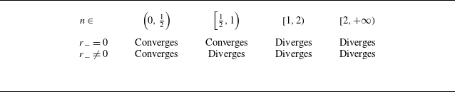
 Λ2(t)
 t→T∗
 n
 r−
 n

 Λ1(t)
 Λ2(t)
 r−=0

 Λ1(t)
 Λ2(t)
 r−∈(0,R]

 n−n+=∞
 Λ1(t)
 Λ2(t)
 t→T∗

 r−=0
 K2+
 L2+
 Δ2t+

 r−∈(0,R]
 n±∈R+
 K1±
 L1±
 Δ1t±

 Open access

