1 Introduction
When a liquid droplet is placed on a flat plate which is either colder or hotter than the ambient atmosphere two major forces drive the fluid motion within the droplet. The thermocapillary effect due to temperature-induced surface-tension variations along the interface causes surface stresses and can drive a significant flow (Scriven & Sternling Reference Scriven and Sternling1960). Furthermore, buoyant forces act in the bulk due to an inhomogeneous thermal expansion of the liquid.
Thermocapillary–buoyant flows in droplets have been studied thoroughly in recent decades due to their importance in many technical applications. An example is the coating of surfaces from binary solutions. Depending on the application either uniform or patterned surface layers are desired. In these processes multiple sequential Marangoni flows can arise as well as particle–surface interactions due to a surfactant-driven Marangoni effect (Kim et al. Reference Kim, Boulogne, Um, Jacobi, Button and Stone2016; Marin et al. Reference Marin, Liepelt, Rossi and Kahler2016). Another application is the so-called lotus effect which was first studied by Johnson & Dettre (Reference Johnson and Dettre1964) using rough hydrophobic surfaces. Technical applications are self-cleaning surfaces due to superhydrophobicity at microscopic and nanoscopic scales (Guo et al. Reference Guo, Zhou, Hao and Liu2005; Cheng et al. Reference Cheng, Rodak, Wong and Hayden2006). A more recent application concerns droplet migration by means of Marangoni convection, which has been treated, e.g. by Chen & Stebe (Reference Chen and Stebe1997), Nguyen & Chen (Reference Nguyen and Chen2010) and Schmitt & Stark (Reference Schmitt and Stark2016), and, more generally, by surface stresses (Darhuber & Troian Reference Darhuber and Troian2005). Further applications are the control of deposition patterns due to droplets ejected by ink-jet printers (Park & Moon Reference Park and Moon2006), droplet and bubble migration under reduced gravity (Wu & Hu Reference Wu and Hu2011) and many more.
The effect of thermocapillarity on droplets and bubbles has been taken into account early in the past century starting with Bond & Newton (Reference Bond and Newton1928). Much later the field became more attractive and many experimental and numerical studies with focus on natural convection, evaporation and Marangoni flows in sessile or hanging droplets have been carried out. Picknett & Bexon (Reference Picknett and Bexon1977) investigated the evaporation of droplets on surfaces experimentally and theoretically and found three general modes of evaporation: constant contact angle, constant radius and the mixed mode, for a large range of contact angles. They also observed that if the evaporation starts with the constant radius, it continues until a certain contact angle and then switches to the constant angle mode. Good & Koo (Reference Good and Koo1979) established an experimental set-up to study the effect of the droplet size on the contact angle employing solid surfaces of different materials. Yekta-Fard & Ponter (Reference Yekta-Fard and Ponter1988) studied the influence of ambient liquid vapour on the contact angle as well as the droplet size. The vigorous interior flow in evaporating droplets was underlined by Hegseth, Rashidnia & Chai (Reference Hegseth, Rashidnia and Chai1996) who established a relation for the droplet lifetime. Mollaret et al. (Reference Mollaret, Sefiane, Christy and Veyret2004) developed a numerical model to describe the hydrodynamics inside the evaporating drop and the effect of the humidity on the evaporation process, assuming the droplet to be a spherical cap. They confirmed the model by comparing the results with their own experiments as well as the previous experimental results. McHale et al. (Reference McHale, Aqil, Shirtcliffe, Newton and Erbil2005) investigated the evaporation of water drops on superhydrophobic surfaces experimentally and observed that the superhydrophobic textured surfaces allow a starting contact angle of more than
 $150^{\circ }$
. In this case the evaporation mode is constant radius initially followed by a step-like contact line retreat. Barash et al. (Reference Barash, Bigioni, Vinokur and Shchur2009) introduced a numerical method to simulate the evaporation of a non-spherical sessile droplet to treat gravity-induced shape deformations. They confirmed, however, that the flow characteristics are well described by the spherical-cap approximation. Numerical simulations of evaporating drops taking into account a moving contact line were carried out by Karapetsas et al. (Reference Karapetsas, Matar, Valluri and Sefiane2012). They observed the formation of stationary cells and travelling hydrothermal waves (Smith & Davis Reference Smith and Davis1983), in qualitative agreement with experimental observations.
The so-called coffee-ring effect was first introduced by Deegan et al. (Reference Deegan, Bakajin, Dupont, Huber, Nagel and Witten1997) who addressed the surface patterns left from the edge of an evaporating droplet containing colloidal particles. Hu & Larson (Reference Hu and Larson2006) showed experimentally and theoretically that the thermocapillary-driven flow reverses the coffee-ring phenomenon and leads to depositions at the droplet centre rather than the edge. Ristenpart et al. (Reference Ristenpart, Kim, Domingues, Wan and Stone2007) considered the thermal conductivity of the substrate and concluded that the direction of the Marangoni flow in a sessile droplet depends on the relative thermal conductivities of the substrate and the liquid, an effect which can significantly alter the resulting particle-deposition patterns. Dunn et al. (Reference Dunn, Wilson, Duffy, David and Sefiane2009) also reported a vigorous influence of substrate conductivity on droplet evaporation using a mathematical model.
An important aspect of the fluid mechanics of liquid droplets is the thermocapillary effect. The influence of thermocapillary-driven flow on the evaporation lifetime of a droplet was investigated numerically by Shih & Megaridis (Reference Shih and Megaridis1996). They showed that the thermocapillary flow amplifies the tangential velocity along the free surface, and consequently enhances the internal circulation within the droplet, which reduces the evaporation lifetime. Savino, Paterna & Favaloro (Reference Savino, Paterna and Favaloro2002) studied buoyancy and thermocapillary effects in hanging evaporating drops comparing the fluid flow for octane, which exhibits the Marangoni effect, and water, in which the thermocapillary effect can be neglected. In their numerical model, they assumed a fixed and undeformable liquid–air interface focusing on small intervals of time at the earlier stages of the evaporation process. Hydrothermal waves in ethanol droplets under normal gravity and microgravity conditions have been investigated by Carle, Sobac & Brutin (Reference Carle, Sobac and Brutin2012) in order to confirm the purely thermocapillary origin of the observed flow instabilities. More recently, Sáenz et al. (Reference Sáenz, Sefiane, Kim, Matar and Valluri2015) studied the evaporation of non-axisymmetric droplets both experimentally and numerically. They reported three-dimensional azimuthal currents in the droplet’s bulk. They also discussed the effect of thermal conduction and thermocapillary convection on the temperature distribution within the droplet for different substrate temperatures.
Many past investigations have focused on the flow and temperature fields, rate of evaporation and, qualitatively, on the interaction among different driving forces within the droplet. Quantitative numerical investigations of the droplet flow are made difficult by the curved and/or moving interface. To circumvent these difficulties we consider the limit of large mean surface tension. By means of orthogonal toroidal coordinates the spherical liquid–gas interface of a droplet of any contact angle can be fitted to a coordinate line. This type of discretisation prevents the necessity of coordinate transforms for droplets of different shapes. The use of toroidal coordinates enables an efficient and accurate numerical treatment of the internal convection in droplets taking into account thermocapillary and buoyant forces. It allows a comprehensive treatment of the problem clarifying, e.g. the role of thermal instabilities for the combined thermocapillary–buoyant convection. A systematic study, moreover, makes possible the identification of scaling laws for asymptotically large Marangoni numbers. Toroidal coordinates have been used before to describe the flow in droplets. These investigations were restricted, however, to the case when the flow is solely driven by evaporation. Evaporation-driven flows have been obtained analytically for inviscid (Masoud & Felske Reference Masoud and Felske2009a ) and for Stokes flows (Masoud & Felske Reference Masoud and Felske2009b ), (see also Kang et al. Reference Kang, Vandadi, Felske and Masoud2016).
We numerically investigate the thermocapillary and buoyant flow in sessile and hanging droplets for a wide range of liquid materials, droplet shapes, levels of gravity, temperature differences as well as heat-transfer coefficients between the liquid and the ambient atmosphere. The problem formulation is provided in § 2 introducing the governing equations and the properties of the coordinate system employed. In § 3 the numerical method is explained and the computational code is verified by means of an exact solution of the Navier–Stokes equations. Numerical results for both sessile and hanging droplets on heated or cooled plates are presented in § 4. The flow structure and its properties are comprehensively studied varying the contact angle and the Reynolds, Prandtl, Biot and Grashof numbers. Finally, § 5 closes with a summary of the results.
2 Problem formulation
We consider a droplet in contact with a plane solid wall which is kept at a constant temperature
 $T_{0}$
. The liquid is assumed incompressible and Newtonian and characterised by its density
 $\unicode[STIX]{x1D70C}$
, surface tension
 $\unicode[STIX]{x1D70E}$
, kinematic viscosity
 $\unicode[STIX]{x1D708}$
and thermal diffusivity
 $\unicode[STIX]{x1D705}$
. The ambient atmosphere is assumed to be a passive gas within which the temperature
 $T_{a}(z)=T_{0}+bz$
varies linearly with the distance
 $z$
from the wall. Owing to the heat transfer between the droplet and ambient gas the surface temperature and thus the surface tension
 $\unicode[STIX]{x1D70E}(T)$
will vary. In a linear approximation
 $\unicode[STIX]{x1D70E}=\unicode[STIX]{x1D70E}_{0}-\unicode[STIX]{x1D6FE}(T-T_{0})$
, where
 $\unicode[STIX]{x1D70E}_{0}$
is the surface tension at the reference (wall) temperature and
 $\unicode[STIX]{x1D6FE}=-\unicode[STIX]{x2202}\unicode[STIX]{x1D70E}/\unicode[STIX]{x2202}T|_{T_{0}}$
the negative surface-tension coefficient. Due to the thermocapillary effect a fluid motion is generated along the interface.
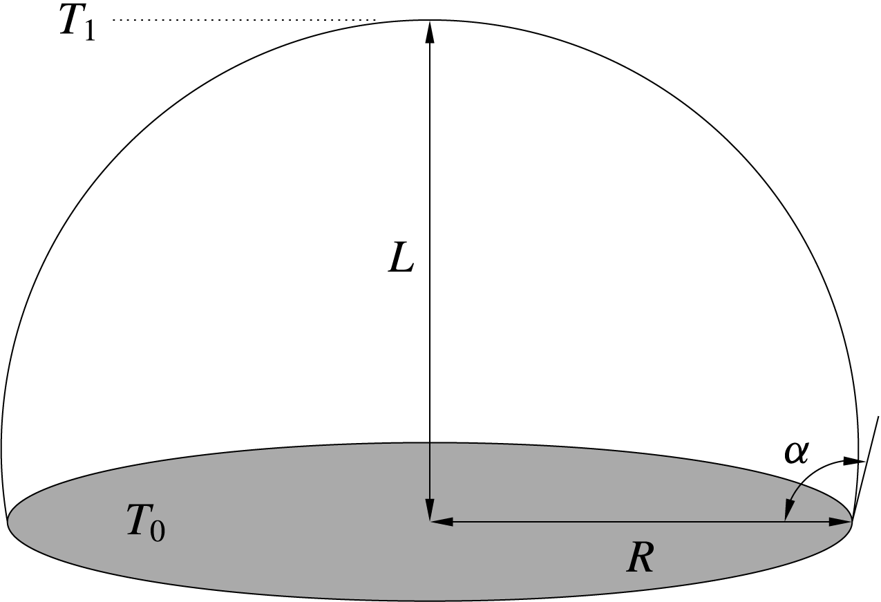
Droplet of height
 $L$
with base radius
 $R$
in contact with a flat plate (grey) at temperature
 $T_{0}$
. The temperature in the passive gas at the level of the droplet’s apex is
 $T_{1}$
. The contact angle
 $\unicode[STIX]{x1D6FC}$
is indicated.

We consider the limit of a non-deformable interface in which the static Bond number
 $Bo=\unicode[STIX]{x1D70C}gL^{2}/\unicode[STIX]{x1D70E}_{0}\rightarrow 0$
vanishes, where
 $L$
is height of the droplet and
 $g$
the acceleration due to gravity which is supposed to be oriented perpendicular to the plate. Furthermore, the limit of vanishingly small capillary number
 $Ca=\unicode[STIX]{x1D6FE}|\unicode[STIX]{x0394}T|/\unicode[STIX]{x1D70E}_{0}\rightarrow 0$
is assumed, where
 $\unicode[STIX]{x0394}T$
, which can be positive or negative, is a measure of the characteristic variation of the temperature of the liquid–gas interface. In this double limit static and dynamic (flow-induced) surface deformations are absent and the liquid–gas interface will be spherical with a circular contact line of radius
 $R$
(see Rienstra Reference Rienstra1990). Figure 1 shows the configuration for a contact angle
 $\unicode[STIX]{x1D6FC}=100^{\circ }$
between droplet and wall. Finally, the liquid is assumed to be non-volatile which renders the domain occupied by the liquid time independent. These assumptions considerably facilitate the calculation of the flow and temperature fields inside the droplet.
2.1 Governing equations
For
 $Bo\rightarrow 0$
and
 $Ca\rightarrow 0$
the flow is governed by the non-dimensional Navier–Stokes, continuity and temperature equations in the Boussinesq approximation
 $$\begin{eqnarray}\displaystyle & \displaystyle Re(\unicode[STIX]{x2202}_{t}+\boldsymbol{U}\boldsymbol{\cdot }\unicode[STIX]{x1D735})\boldsymbol{U}=-\unicode[STIX]{x1D735}P+\unicode[STIX]{x1D6FB}^{2}\boldsymbol{U}+\frac{Gr}{Re}\unicode[STIX]{x1D703}\boldsymbol{k}, & \displaystyle\end{eqnarray}$$
 $$\begin{eqnarray}\displaystyle & \displaystyle \unicode[STIX]{x1D735}\boldsymbol{\cdot }\boldsymbol{U}=0, & \displaystyle\end{eqnarray}$$
 $$\begin{eqnarray}\displaystyle & \displaystyle Re\,Pr(\unicode[STIX]{x2202}_{t}+\boldsymbol{U}\boldsymbol{\cdot }\unicode[STIX]{x1D735})\unicode[STIX]{x1D703}=\unicode[STIX]{x1D6FB}^{2}\unicode[STIX]{x1D703}, & \displaystyle\end{eqnarray}$$
 $U^{\star }$
being the characteristic thermocapillary velocity. The temperature is scaled by
 $\unicode[STIX]{x0394}T=|T_{1}-T_{0}|$
, where
 $T_{1}=bL$
is the temperature in the ambient atmosphere at the apex of the droplet located at a distance
 $L$
above the plate. Defining the mean temperature
 $T_{m}=(T_{0}+T_{1})/2$
we consider the reduced temperature
 $\unicode[STIX]{x1D703}=(T-T_{m})/\unicode[STIX]{x0394}T+1/2$
. The definition is such that the temperature distribution in the ambient atmosphere is
 $\unicode[STIX]{x1D703}_{a}(z=0)=\unicode[STIX]{x1D703}_{0}=0$
and
 $\unicode[STIX]{x1D703}_{a}(z=l)=1$
in the case of a cold plate in a hot environment and
 $\unicode[STIX]{x1D703}_{a}(z=0)=\unicode[STIX]{x1D703}_{0}=1$
and
 $\unicode[STIX]{x1D703}_{a}(z=l)=0$
in the case of a hot plate in a cold environment, where
 $l=L/R$
is the scaled height (aspect ratio) of the droplet.
The dimensionless parameters in (2.1) are
 $$\begin{eqnarray}Re=\frac{U^{\star }R}{\unicode[STIX]{x1D708}}=\frac{\unicode[STIX]{x1D6FE}\unicode[STIX]{x0394}TR}{\unicode[STIX]{x1D70C}\unicode[STIX]{x1D708}^{2}},\quad Pr=\frac{\unicode[STIX]{x1D708}}{\unicode[STIX]{x1D705}},\quad Gr=\frac{g\unicode[STIX]{x1D6FD}\unicode[STIX]{x0394}TR^{3}}{\unicode[STIX]{x1D708}^{2}},\end{eqnarray}$$
where
 $\unicode[STIX]{x1D6FD}=-\unicode[STIX]{x1D70C}^{-1}\unicode[STIX]{x2202}\unicode[STIX]{x1D70C}/\unicode[STIX]{x2202}T|_{p}$
is the isobaric thermal expansion coefficient of the liquid. On the flat plate we impose no-slip conditions
 $\boldsymbol{U}=0$
and a constant temperature of
 $\unicode[STIX]{x1D703}=1$
or
 $\unicode[STIX]{x1D703}=0$
, respectively, in the case of heating or cooling from the plate.
Scaling of the variables with
 $Re$
according to (2.2).

In the absence of mass transfer at the interface the normal velocity must vanish on the interface, i.e.
 $\boldsymbol{U}\boldsymbol{\cdot }\boldsymbol{n}=0$
. Furthermore, thermocapillary stresses on the interface must be balanced by tangential viscous stresses
 $$\begin{eqnarray}\boldsymbol{t}\boldsymbol{\cdot }(\unicode[STIX]{x1D64E}\boldsymbol{\cdot }\boldsymbol{n})=-\boldsymbol{t}\boldsymbol{\cdot }\unicode[STIX]{x1D735}\unicode[STIX]{x1D703},\end{eqnarray}$$
where
 $\unicode[STIX]{x1D64E}=\unicode[STIX]{x1D735}\boldsymbol{U}+(\unicode[STIX]{x1D735}\boldsymbol{U})^{\text{T}}$
is the viscous stress tensor in the liquid phase,
 $\boldsymbol{n}$
and
 $\boldsymbol{t}$
are the unit normal and tangent vectors to the interface and viscous stresses in the gas phase have been neglected.
The heat transfer between the droplet and the ambient gas is modelled using Newton’s law
 $$\begin{eqnarray}\boldsymbol{n}\boldsymbol{\cdot }\unicode[STIX]{x1D735}\unicode[STIX]{x1D703}=-Bi(\unicode[STIX]{x1D703}-\unicode[STIX]{x1D703}_{a}),\quad \text{with }\unicode[STIX]{x1D703}_{a}(z)=\left\{\begin{array}{@{}ll@{}}1-z/l, & \text{if }b<0\text{ (hot plate)},\\ z/l, & \text{if }b>0\text{(cold plate)},\end{array}\right.\end{eqnarray}$$
where
 $Bi=hR/k$
is the Biot number with heat-transfer coefficient
 $h$
and
 $k$
the thermal conductivity.
2.2 Toroidal coordinates
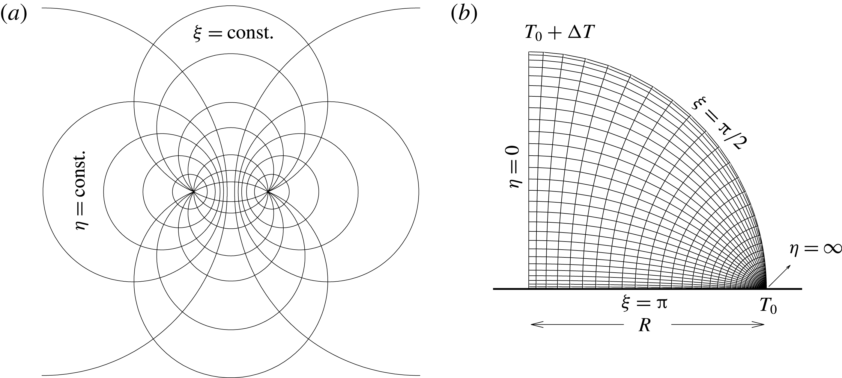
For a numerical treatment of the problem body-fitted coordinates are of great advantage. Since the interface is a spherical cap, we use toroidal coordinates (
 $\unicode[STIX]{x1D702},\unicode[STIX]{x1D709},\unicode[STIX]{x1D719}$
). As can be seen from figure 2(a) the spherical interface of the droplet coincides with a coordinate line, independent of the contact angle.
(a) Toroidal coordinates. (b) A coarse non-uniform mesh corresponding to toroidal coordinates
 $(\unicode[STIX]{x1D702},\unicode[STIX]{x1D709})$
.

Toroidal coordinates are obtained by rotating planar bipolar coordinates about the
 $y$
-axis (Arfken Reference Arfken1985). The coordinates have two foci which are located at
 $(\pm a,0)$
. The transformation equations between Cartesian and toroidal coordinates as well as the scale factors are (here given in three dimensions)
 $$\begin{eqnarray}x=\frac{a\sinh \unicode[STIX]{x1D702}\cos \unicode[STIX]{x1D719}}{\cosh \unicode[STIX]{x1D702}-\cos \unicode[STIX]{x1D709}},\quad y=\frac{a\sinh \unicode[STIX]{x1D702}\sin \unicode[STIX]{x1D719}}{\cosh \unicode[STIX]{x1D702}-\cos \unicode[STIX]{x1D709}},\quad z=\frac{a\sin \unicode[STIX]{x1D709}}{\cosh \unicode[STIX]{x1D702}-\cos \unicode[STIX]{x1D709}},\end{eqnarray}$$
 $$\begin{eqnarray}h_{\unicode[STIX]{x1D702}}=h_{\unicode[STIX]{x1D709}}=\frac{a}{\cosh \unicode[STIX]{x1D702}-\cos \unicode[STIX]{x1D709}},\quad h_{\unicode[STIX]{x1D719}}=\frac{a\sinh \unicode[STIX]{x1D702}}{\cosh \unicode[STIX]{x1D702}-\cos \unicode[STIX]{x1D709}},\end{eqnarray}$$
and the unit vectors
 $(\boldsymbol{e}_{\unicode[STIX]{x1D702}},\boldsymbol{e}_{\unicode[STIX]{x1D709}},\boldsymbol{e}_{\unicode[STIX]{x1D719}})$
can be expressed by the Cartesian unit vectors
 $(\boldsymbol{i},\boldsymbol{j},\boldsymbol{k})$
using
 $$\begin{eqnarray}\displaystyle & \displaystyle \boldsymbol{e}_{\unicode[STIX]{x1D702}}=\frac{\cos \unicode[STIX]{x1D719}(1-\cosh \unicode[STIX]{x1D702}\cos \unicode[STIX]{x1D709})}{q}\boldsymbol{i}+\frac{\sin \unicode[STIX]{x1D719}(1-\cosh \unicode[STIX]{x1D702}\cos \unicode[STIX]{x1D709})}{q}\boldsymbol{j}-\frac{\sinh \unicode[STIX]{x1D702}\sin \unicode[STIX]{x1D709}}{q}\boldsymbol{k},\quad & \displaystyle\end{eqnarray}$$
 $$\begin{eqnarray}\displaystyle & \displaystyle \boldsymbol{e}_{\unicode[STIX]{x1D709}}=-\frac{\sinh \unicode[STIX]{x1D702}\sin \unicode[STIX]{x1D709}\cos \unicode[STIX]{x1D719}}{q}\boldsymbol{i}-\frac{\sinh \unicode[STIX]{x1D702}\sin \unicode[STIX]{x1D709}\sin \unicode[STIX]{x1D719}}{q}\boldsymbol{j}+\frac{\cosh \unicode[STIX]{x1D702}\cos \unicode[STIX]{x1D709}-1}{q}\boldsymbol{k}, & \displaystyle\end{eqnarray}$$
 $$\begin{eqnarray}\displaystyle & \displaystyle \boldsymbol{e}_{\unicode[STIX]{x1D719}}=-\!\sin \unicode[STIX]{x1D719}\boldsymbol{i}+\cos \unicode[STIX]{x1D719}\boldsymbol{j}, & \displaystyle\end{eqnarray}$$
 $q=\cosh \unicode[STIX]{x1D702}-\cos \unicode[STIX]{x1D709}$
. The vector operators gradient, divergence, curl and Laplacian, respectively, are written as
 $$\begin{eqnarray}\displaystyle & \displaystyle \unicode[STIX]{x1D735}\unicode[STIX]{x1D713}=\frac{q}{a}\left(\boldsymbol{e}_{\unicode[STIX]{x1D702}}\frac{\unicode[STIX]{x2202}\unicode[STIX]{x1D713}}{\unicode[STIX]{x2202}\unicode[STIX]{x1D702}}+\boldsymbol{e}_{\unicode[STIX]{x1D709}}\frac{\unicode[STIX]{x2202}\unicode[STIX]{x1D713}}{\unicode[STIX]{x2202}\unicode[STIX]{x1D709}}+\boldsymbol{e}_{\unicode[STIX]{x1D719}}\frac{1}{\sinh \unicode[STIX]{x1D702}}\frac{\unicode[STIX]{x2202}\unicode[STIX]{x1D713}}{\unicode[STIX]{x2202}\unicode[STIX]{x1D719}}\right), & \displaystyle\end{eqnarray}$$
 $$\begin{eqnarray}\displaystyle & \displaystyle \unicode[STIX]{x1D735}\boldsymbol{\cdot }\boldsymbol{U}=\frac{q}{a}\left[\frac{\unicode[STIX]{x2202}U_{\unicode[STIX]{x1D702}}}{\unicode[STIX]{x2202}\unicode[STIX]{x1D702}}+\frac{\unicode[STIX]{x2202}U_{\unicode[STIX]{x1D709}}}{\unicode[STIX]{x2202}\unicode[STIX]{x1D709}}+\frac{1}{\sinh \unicode[STIX]{x1D702}}\frac{\unicode[STIX]{x2202}U_{\unicode[STIX]{x1D719}}}{\unicode[STIX]{x2202}\unicode[STIX]{x1D719}}-2U_{\unicode[STIX]{x1D709}}\frac{\sin \unicode[STIX]{x1D709}}{q}+U_{\unicode[STIX]{x1D702}}\left(\frac{\cosh \unicode[STIX]{x1D702}}{\sinh \unicode[STIX]{x1D702}}-\frac{2\sinh \unicode[STIX]{x1D702}}{q}\right)\right], & \displaystyle \nonumber\\ \displaystyle & & \displaystyle\end{eqnarray}$$
 $$\begin{eqnarray}\displaystyle & \displaystyle \unicode[STIX]{x1D735}\times \boldsymbol{U}=\frac{q^{3}}{a^{3}\sinh \unicode[STIX]{x1D702}}\left|\begin{array}{@{}ccc@{}}\boldsymbol{e}_{\unicode[STIX]{x1D702}}(a/q) & \boldsymbol{e}_{\unicode[STIX]{x1D709}}(a/q) & \boldsymbol{e}_{\unicode[STIX]{x1D719}}(a/q)\sinh \unicode[STIX]{x1D702}\\ \unicode[STIX]{x2202}_{\unicode[STIX]{x1D702}} & \unicode[STIX]{x2202}_{\unicode[STIX]{x1D709}} & \unicode[STIX]{x2202}_{\unicode[STIX]{x1D719}}\\ (a/q)U_{\unicode[STIX]{x1D702}} & (a/q)U_{\unicode[STIX]{x1D709}} & (a/q)\sinh \unicode[STIX]{x1D702}U_{\unicode[STIX]{x1D719}}\end{array}\right|, & \displaystyle\end{eqnarray}$$
 $$\begin{eqnarray}\displaystyle & \displaystyle \unicode[STIX]{x1D6FB}^{2}\unicode[STIX]{x1D713}=\frac{q^{2}}{a^{2}}\left[\unicode[STIX]{x2202}_{\unicode[STIX]{x1D702}\unicode[STIX]{x1D702}}\unicode[STIX]{x1D713}+\unicode[STIX]{x2202}_{\unicode[STIX]{x1D709}\unicode[STIX]{x1D709}}\unicode[STIX]{x1D713}+\frac{1}{\sinh ^{2}\unicode[STIX]{x1D702}}\unicode[STIX]{x2202}_{\unicode[STIX]{x1D719}\unicode[STIX]{x1D719}}\unicode[STIX]{x1D713}-\left(\frac{\cosh \unicode[STIX]{x1D702}\cos \unicode[STIX]{x1D709}-1}{q\sinh \unicode[STIX]{x1D702}}\right)\unicode[STIX]{x2202}_{\unicode[STIX]{x1D702}}\unicode[STIX]{x1D713}-\frac{\sin \unicode[STIX]{x1D709}}{q}\unicode[STIX]{x2202}_{\unicode[STIX]{x1D709}}\unicode[STIX]{x1D713}\right], & \displaystyle \nonumber\\ \displaystyle & & \displaystyle\end{eqnarray}$$
 $\boldsymbol{U}=(U_{\unicode[STIX]{x1D702}},U_{\unicode[STIX]{x1D709}},U_{\unicode[STIX]{x1D719}})$
is the (velocity) vector in toroidal coordinates. These expressions are used to formulate the Navier–Stokes and energy equations in toroidal coordinates. The coordinates are illustrated in figure 2(b) for a contact angle
 $\unicode[STIX]{x1D6FC}=\unicode[STIX]{x03C0}/2$
and constant
 $\unicode[STIX]{x1D719}$
. The focus coordinate is given by the non-dimensional radius of the base such that
 $a=1$
. The contact angle can be expressed as a function of the interface coordinate
 $\unicode[STIX]{x1D709}_{min}$
as
 $$\begin{eqnarray}\unicode[STIX]{x1D6FC}(\unicode[STIX]{x1D709}_{min})=\unicode[STIX]{x03C0}-\unicode[STIX]{x1D709}_{min}.\end{eqnarray}$$
2.3 Steady axisymmetric flow
The steady axisymmetric boundary conditions allow for a steady axisymmetric basic flow. For
 $\unicode[STIX]{x2202}_{t}=U_{\unicode[STIX]{x1D719}}=\unicode[STIX]{x2202}_{\unicode[STIX]{x1D719}}=0$
the flow only depends on
 $\unicode[STIX]{x1D709}$
and
 $\unicode[STIX]{x1D702}$
. Therefore, we introduce the streamfunction
 $\unicode[STIX]{x1D6F9}$
by
 $$\begin{eqnarray}\displaystyle & \displaystyle U_{\unicode[STIX]{x1D702}}=\frac{q^{2}}{\sinh \unicode[STIX]{x1D702}}\frac{\unicode[STIX]{x2202}\unicode[STIX]{x1D6F9}}{\unicode[STIX]{x2202}\unicode[STIX]{x1D709}}, & \displaystyle\end{eqnarray}$$
 $$\begin{eqnarray}\displaystyle & \displaystyle U_{\unicode[STIX]{x1D709}}=-\frac{q^{2}}{\sinh \unicode[STIX]{x1D702}}\frac{\unicode[STIX]{x2202}\unicode[STIX]{x1D6F9}}{\unicode[STIX]{x2202}\unicode[STIX]{x1D702}}, & \displaystyle\end{eqnarray}$$
 $\boldsymbol{U}$
is tangent to the isolines
 $\unicode[STIX]{x1D6F9}=\text{const.}$
or, equivalently,
 $\boldsymbol{U}\boldsymbol{\cdot }\unicode[STIX]{x1D735}\unicode[STIX]{x1D6F9}=0$
. Thus
 $\unicode[STIX]{x1D6F9}$
is the Stokes streamfunction.
The vorticity is
 $$\begin{eqnarray}\unicode[STIX]{x1D6FA}=-\frac{q^{3}}{\sinh \unicode[STIX]{x1D702}}\left[\unicode[STIX]{x2202}_{\unicode[STIX]{x1D702}\unicode[STIX]{x1D702}}+\unicode[STIX]{x2202}_{\unicode[STIX]{x1D709}\unicode[STIX]{x1D709}}+\frac{\cosh \unicode[STIX]{x1D702}\cos \unicode[STIX]{x1D709}-1}{q\sinh \unicode[STIX]{x1D702}}\unicode[STIX]{x2202}_{\unicode[STIX]{x1D702}}+\frac{\sin \unicode[STIX]{x1D709}}{q}\unicode[STIX]{x2202}_{\unicode[STIX]{x1D709}}\right]\unicode[STIX]{x1D6F9}.\end{eqnarray}$$
Taking the curl of (2.1a ) to eliminate the pressure we obtain the momentum and temperature equations in the form
 $$\begin{eqnarray}\displaystyle & & \displaystyle q^{2}\left[\unicode[STIX]{x2202}_{\unicode[STIX]{x1D702}\unicode[STIX]{x1D702}}+\unicode[STIX]{x2202}_{\unicode[STIX]{x1D709}\unicode[STIX]{x1D709}}-\frac{\cosh \unicode[STIX]{x1D702}\cos \unicode[STIX]{x1D709}-1}{q\sinh \unicode[STIX]{x1D702}}\unicode[STIX]{x2202}_{\unicode[STIX]{x1D702}}-\frac{\sin \unicode[STIX]{x1D709}}{q}\unicode[STIX]{x2202}_{\unicode[STIX]{x1D709}}\right]\unicode[STIX]{x1D6FA}=Re\frac{q^{3}}{\sinh \unicode[STIX]{x1D702}}(\unicode[STIX]{x2202}_{\unicode[STIX]{x1D709}}\unicode[STIX]{x1D6F9}\unicode[STIX]{x2202}_{\unicode[STIX]{x1D702}}-\unicode[STIX]{x2202}_{\unicode[STIX]{x1D702}}\unicode[STIX]{x1D6F9}\unicode[STIX]{x2202}_{\unicode[STIX]{x1D709}})\unicode[STIX]{x1D6FA}\nonumber\\ \displaystyle & & \displaystyle \quad -\,\frac{Gr}{Re}[(\cosh \unicode[STIX]{x1D702}\cos \unicode[STIX]{x1D709}-1)\unicode[STIX]{x2202}_{\unicode[STIX]{x1D702}}+(\sinh \unicode[STIX]{x1D702}\sin \unicode[STIX]{x1D709})\unicode[STIX]{x2202}_{\unicode[STIX]{x1D709}}]\unicode[STIX]{x1D703},\end{eqnarray}$$
 $$\begin{eqnarray}\left[\unicode[STIX]{x2202}_{\unicode[STIX]{x1D702}\unicode[STIX]{x1D702}}+\unicode[STIX]{x2202}_{\unicode[STIX]{x1D709}\unicode[STIX]{x1D709}}-\frac{\cosh \unicode[STIX]{x1D702}\cos \unicode[STIX]{x1D709}-1}{q\sinh \unicode[STIX]{x1D702}}\unicode[STIX]{x2202}_{\unicode[STIX]{x1D702}}-\frac{\sin \unicode[STIX]{x1D709}}{q}\unicode[STIX]{x2202}_{\unicode[STIX]{x1D709}}\right]\unicode[STIX]{x1D703}=Ma\frac{q}{\sinh \unicode[STIX]{x1D702}}(\unicode[STIX]{x2202}_{\unicode[STIX]{x1D709}}\unicode[STIX]{x1D6F9}\unicode[STIX]{x2202}_{\unicode[STIX]{x1D702}}-\unicode[STIX]{x2202}_{\unicode[STIX]{x1D702}}\unicode[STIX]{x1D6F9}\unicode[STIX]{x2202}_{\unicode[STIX]{x1D709}})\unicode[STIX]{x1D703},\end{eqnarray}$$
where the Marangoni number is defined as
 $Ma=Re\,Pr=U^{\star }R/\unicode[STIX]{x1D705}$
, acting as a Péclet number. The streamfunction, vorticity and temperature fields must satisfy the boundary conditions
 $$\begin{eqnarray}\displaystyle & \displaystyle \unicode[STIX]{x2202}_{\unicode[STIX]{x1D702}}\unicode[STIX]{x1D703}=0,\quad \unicode[STIX]{x1D6F9}=\unicode[STIX]{x1D6FA}=0,\quad \text{on }\unicode[STIX]{x1D702}=0\text{ (vertical axis),} & \displaystyle\end{eqnarray}$$
 $$\begin{eqnarray}\displaystyle & \displaystyle \unicode[STIX]{x1D703}=\unicode[STIX]{x1D703}_{0},\quad \unicode[STIX]{x1D6F9}=\unicode[STIX]{x2202}_{\unicode[STIX]{x1D702}}\unicode[STIX]{x1D6F9}=0,\quad \text{on }\unicode[STIX]{x1D702}\rightarrow \infty \text{(contact line),} & \displaystyle\end{eqnarray}$$
 $$\begin{eqnarray}\displaystyle & \displaystyle \unicode[STIX]{x1D703}=\unicode[STIX]{x1D703}_{0},\quad \unicode[STIX]{x1D6F9}=\unicode[STIX]{x2202}_{\unicode[STIX]{x1D709}}\unicode[STIX]{x1D6F9}=0,\quad \text{on }\unicode[STIX]{x1D709}=\unicode[STIX]{x03C0}\text{ (bottom plate).} & \displaystyle\end{eqnarray}$$
On the spherical free surface we impose
 $$\begin{eqnarray}\left.\begin{array}{@{}c@{}}\displaystyle \unicode[STIX]{x1D6F9}=0,\\ \displaystyle \unicode[STIX]{x2202}_{\unicode[STIX]{x1D709}}\unicode[STIX]{x1D703}=Bi(\unicode[STIX]{x1D703}-\unicode[STIX]{x1D703}_{a}),\\ \displaystyle \unicode[STIX]{x1D6FA}=-\unicode[STIX]{x2202}_{\unicode[STIX]{x1D702}}\unicode[STIX]{x1D703}+\displaystyle \frac{2q^{2}\sin \unicode[STIX]{x1D709}}{\sinh \unicode[STIX]{x1D702}}\unicode[STIX]{x2202}_{\unicode[STIX]{x1D709}}\unicode[STIX]{x1D6F9}\end{array}\right\}\quad \text{on }\unicode[STIX]{x1D709}=\unicode[STIX]{x1D709}_{min}\text{ (free surface)}.\end{eqnarray}$$
3 Numerical solution and code verification
Toroidal coordinates exhibit a singularity at the three-phase contact line where
 $\unicode[STIX]{x1D702}\rightarrow \infty$
. In order to manage this coordinate singularity numerically we truncate the full range
 $\unicode[STIX]{x1D702}\in [0,\infty ]$
to
 $\unicode[STIX]{x1D702}\in [0,\unicode[STIX]{x1D702}_{max}]$
with
 $\unicode[STIX]{x1D702}_{max}=6.5$
sufficiently large. As a result a circular segment with a very small radius of
 $1-\sinh \unicode[STIX]{x1D702}_{max}/(1+\cosh \unicode[STIX]{x1D702}_{max})=3.00\times 10^{-3}$
around the triple point is excluded from the computational domain. Along
 $\unicode[STIX]{x1D702}=\unicode[STIX]{x1D702}_{max}$
no slip and wall temperature conditions are imposed. Equations (2.10a
)–(2.10c
) are then discretised using second-order central finite differences on a non-uniform toroidal grid (see figure 2
b). The discontinuity of the boundary conditions is not affected and remains located at
 $(\unicode[STIX]{x1D702},\unicode[STIX]{x1D709})=(\unicode[STIX]{x1D702}_{max},\unicode[STIX]{x1D709}_{min})$
. As in similar investigations this integrable singularity is regularised by the filtering imposed by the finite-difference method.
The system of nonlinear equations is solved by Newton–Raphson iteration implemented within a Matlab code. Under-relaxation is applied to stabilise the iteration. The resulting linear equations are solved using Matlab’s backslash operator.
The value of
 $\unicode[STIX]{x1D702}_{max}$
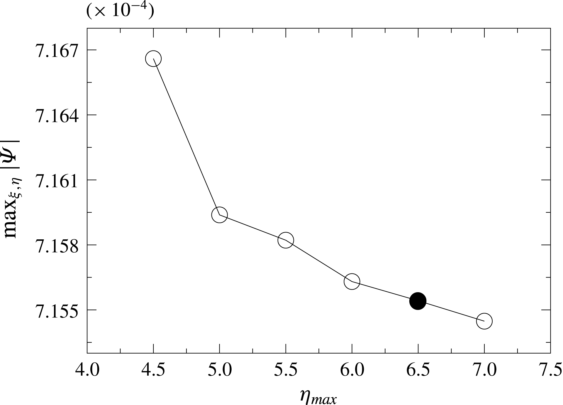
has been selected based on a trade-off between minimising the cutout area and to prevent an excessive accumulation of grid points. The effect of the cutoff length
 $\unicode[STIX]{x1D702}_{max}$
on the maximum absolute value of the streamfunction is shown in figure 3 for a test case. As can be seen
 $\text{max}\,|\unicode[STIX]{x1D6F9}|$
levels off for increasing
 $\unicode[STIX]{x1D702}_{max}$
. A further increase of
 $\unicode[STIX]{x1D702}_{max}$
would lead to an unnecessary grid refinement close to the three-phase point. As a compromise
 $\unicode[STIX]{x1D702}_{max}=6.5$
was selected.
Maximum
 $\max _{\unicode[STIX]{x1D709},\unicode[STIX]{x1D702}}|\unicode[STIX]{x1D6F9}|$
as a function of
 $\unicode[STIX]{x1D702}_{max}$
. The parameters are
 $Re=100,Pr=4,Gr=0,Bi=0.1$
and
 $\unicode[STIX]{x1D6FC}=\unicode[STIX]{x03C0}/2$
. The full dot indicates the selected cutoff
 $\unicode[STIX]{x1D702}_{max}=6.5$
. Note the relative range of the ordinate.

To verify the correct implementation of the discrete momentum equations numerical results are compared with the Kovasznay flow (Kovasznay Reference Kovasznay1948) which is an exact closed-form solution of the steady two-dimensional Navier–Stokes equations. The Kovasznay flow reads
 $$\begin{eqnarray}\displaystyle & \displaystyle \unicode[STIX]{x1D6F9}=y-\frac{\text{e}^{\unicode[STIX]{x1D706}x}}{2\unicode[STIX]{x03C0}}\sin 2\unicode[STIX]{x03C0}y, & \displaystyle\end{eqnarray}$$
 $$\begin{eqnarray}\displaystyle & \displaystyle \unicode[STIX]{x1D6FA}=\frac{\unicode[STIX]{x1D706}^{2}-4\unicode[STIX]{x03C0}^{2}}{2\unicode[STIX]{x03C0}}\text{e}^{\unicode[STIX]{x1D706}x}\sin 2\unicode[STIX]{x03C0}y, & \displaystyle\end{eqnarray}$$
 $\unicode[STIX]{x1D706}=(Re/2)-\sqrt{4\unicode[STIX]{x03C0}^{2}+(Re^{2}/4)}$
.
In order to treat such plane flow we modified the numerical implementation to plane bipolar coordinates rather than toroidal. For the verification we selected a domain in the bipolar plane bounded by arbitrary coordinate lines. Here we use
 $\unicode[STIX]{x1D709}\times \unicode[STIX]{x1D702}\in [\unicode[STIX]{x03C0}/2,3\unicode[STIX]{x03C0}/2]\times [-1.5,2.25]$
. For the numerical computations a uniform grid in both
 $\unicode[STIX]{x1D702}$
and
 $\unicode[STIX]{x1D709}$
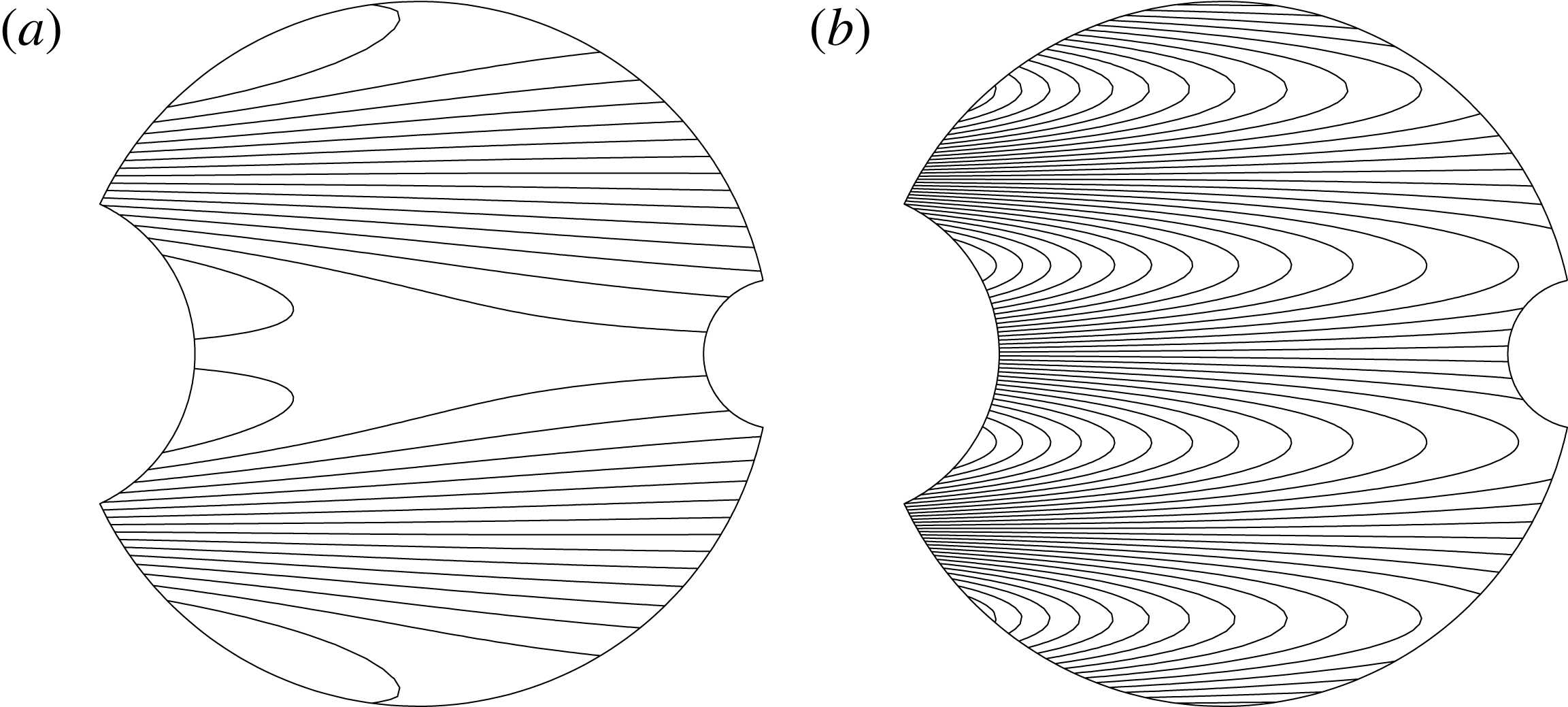
directions is employed. Dirichlet boundary conditions for the streamfunction and vorticity are specified on all boundaries using the exact solution (3.1). Computed streamline and vorticity contours within this domain are shown in figure 4. The contour lines visually agree with those for the exact solution.
Computed streamfunction (a) and vorticity (b) for the Kovasznay flow at
 $Re=40$
in the domain
 $\unicode[STIX]{x1D709}\times \unicode[STIX]{x1D702}\in [\unicode[STIX]{x03C0}/2,3\unicode[STIX]{x03C0}/2]\times [-1.5,2.25]$
.

To show grid convergence, calculations were carried out for different grid sizes, from
 $40\times 40$
up to
 $240\times 240$
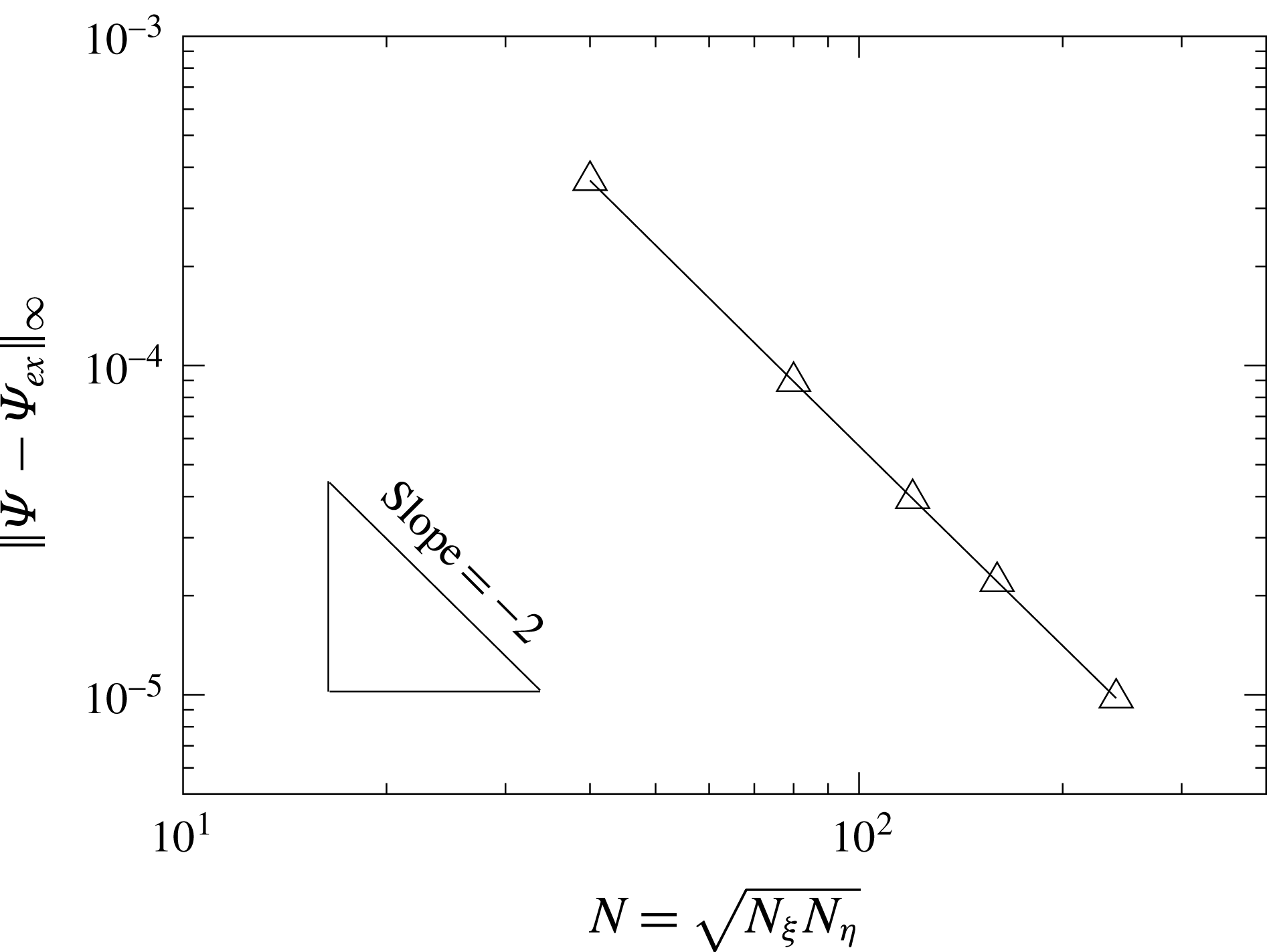
. Figure 5 shows the infinity norm of the deviation of the computed streamfunction from the exact solution as a function of the grid size. The slope of the curve confirms the second-order convergence rate of the numerical scheme.
Infinity norm of the numerical error of
 $\unicode[STIX]{x1D6F9}$
(deviation from the exact streamfunction
 $\unicode[STIX]{x1D6F9}_{ex}$
of the Kovasznay flow (3.1)) on an equidistant grid as a function of the root mean number of grid points for
 $N_{\unicode[STIX]{x1D709}}=N_{\unicode[STIX]{x1D702}}$
.

The energy equation is verified by considering a creeping flow (
 $Re\rightarrow 0$
) in the absence of gravity (
 $Gr=0$
) in the sessile droplet with
 $Bi\rightarrow \infty$
(imposed surface temperature
 $\unicode[STIX]{x1D703}_{a}=1-z/l$
). With these assumptions the convective heat transfer is negligible. The solution of the temperature equation yields the conducting state as required (see the isotherms illustrated in figure 13
e).
Finally, a grid refinement study is performed. To take into account of the developing boundary layers the grid is stretched towards all boundaries using
 $$\begin{eqnarray}\displaystyle & \displaystyle \unicode[STIX]{x1D702}=12.26\;[\tanh ^{-1}(x_{1})]^{1.06},\quad x_{1}\in [0,0.5], & \displaystyle\end{eqnarray}$$
 $$\begin{eqnarray}\displaystyle & \displaystyle \unicode[STIX]{x1D709}=\unicode[STIX]{x1D709}_{mid}+\tanh (x_{2}),\quad x_{2}\in [\tanh ^{-1}(-\unicode[STIX]{x1D709}_{sym}),\tanh ^{-1}(\unicode[STIX]{x1D709}_{sym})], & \displaystyle\end{eqnarray}$$
 $N_{\unicode[STIX]{x1D702}}$
and
 $N_{\unicode[STIX]{x1D709}}$
points in the intervals of
 $x_{1}$
and
 $x_{2}$
, respectively. The intervals of
 $x_{1}$
and
 $x_{2}$
are mapped to
 $\unicode[STIX]{x1D702}\in [0,6.5]$
and
 $\unicode[STIX]{x1D709}\in [\unicode[STIX]{x1D709}_{min},\unicode[STIX]{x1D709}_{max}]$
, where the solid wall is represented by
 $\unicode[STIX]{x1D709}_{max}=\unicode[STIX]{x03C0}$
and
 $\unicode[STIX]{x1D709}_{min}$
depends on the contact angle. The grid in
 $\unicode[STIX]{x1D709}$
is stretched symmetrically from the midpoint
 $\unicode[STIX]{x1D709}_{mid}=(\unicode[STIX]{x1D709}_{max}+\unicode[STIX]{x1D709}_{min})/2$
by defining
 $\unicode[STIX]{x1D709}_{sym}=(\unicode[STIX]{x1D709}_{max}-\unicode[STIX]{x1D709}_{min})/2$
. The mapping (3.2) ensures that the stretching factor is always in the range
 $[0.9,1.1]$
.
To assess grid convergence the extrema of the Stokes streamfunction,
 $|\unicode[STIX]{x1D6F9}|_{max}$
, as well as the vorticity at the location of the streamfunction extrema,
 $\unicode[STIX]{x1D6FA}_{core}$
, are monitored. Based on the results listed in table 2 a grid size of
 $N_{\unicode[STIX]{x1D702}}\times N_{\unicode[STIX]{x1D709}}=200\times 100$
has been selected for all further computations, except for cases in which thin thermal boundary layers call for a higher resolution. In such cases, finer grids up to
 $N_{\unicode[STIX]{x1D702}}\times N_{\unicode[STIX]{x1D709}}=400\times 200$
are employed.
Extrema
 $|\unicode[STIX]{x1D6F9}|_{max}$
of the Stokes streamfunction and vorticity
 $\unicode[STIX]{x1D6FA}_{core}$
at the locations of the streamfunction extrema for different non-uniform grids
 $N_{\unicode[STIX]{x1D702}}\times N_{\unicode[STIX]{x1D709}}$
. The parameters are
 $Re=100$
,
 $Bi=0.1$
and
 $Gr=0$
.

4 Results
The numerical steady states have been calculated varying
 $Re$
,
 $Pr$
,
 $Gr$
,
 $Bi$
as well as the contact angle
 $\unicode[STIX]{x1D6FC}$
. Results are provided in form of streamfunction and temperature isolines which are shown in the left and right quadrant, respectively, in the following graphs.
4.1 Heated plate
4.1.1 Thermocapillary-driven flow
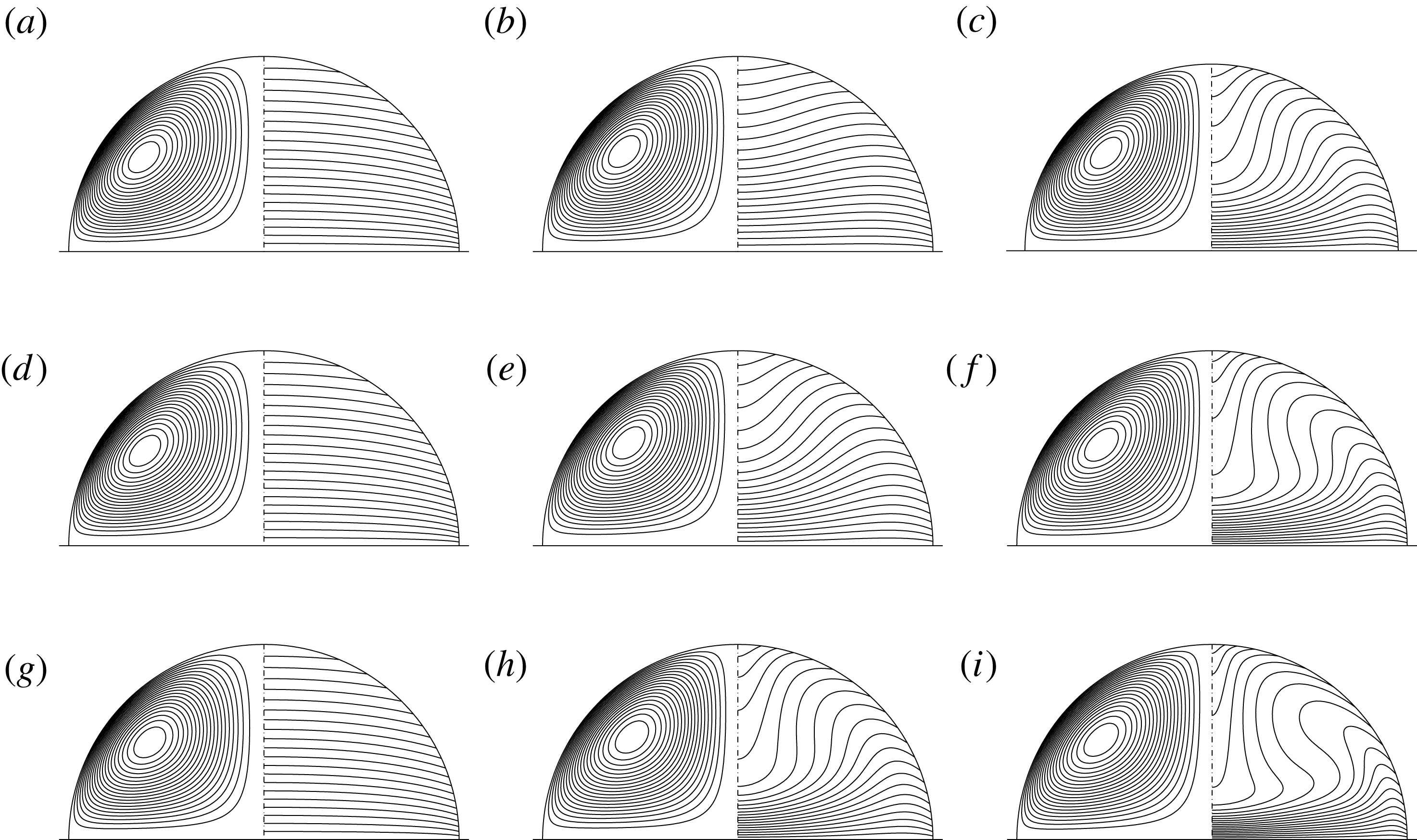
Figure 6 shows the influence of the Reynolds number on the flow patterns for three different Prandtl numbers (columns) and three Reynolds numbers (rows) in the absence of gravity. For
 $Pr=0.02$
and up to
 $Re=1000$
the thermocapillary flow has little effect on the temperature field. For
 $Pr=4$
and 28, however, convective effects are clearly visible with a tendency to develop thermal boundary layers on the heated plate.
Reynolds number variation for
 $Pr=0.02$
(a,d,g),
 $Pr=4$
(b,e,h) and
 $Pr=28$
(c,f,i), for
 $Gr=0$
and
 $Bi=0.1$
. (a–c)
 $Re=100$
, (d–f)
 $Re=250$
, (g–i)
 $Re=1000$
. For each droplet: streamlines (left quadrants) and isotherms (right quadrants).

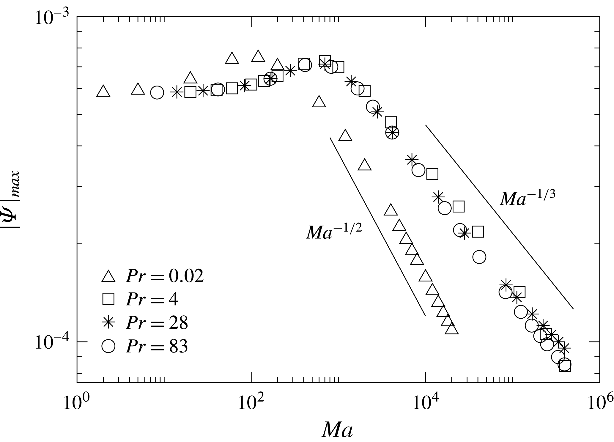
Maximum of
 $|\unicode[STIX]{x1D6F9}|$
as a function of
 $Ma$
for thermocapillary flow in a droplet on a heated plate (thermocapillary scaling, see table 1). The parameters are
 $Gr=0$
and
 $Bi=0.1$
.

Figure 7 shows the strength of the flow expressed by the absolute streamfunction extremum as a function of the Marangoni number. In all cases
 $\unicode[STIX]{x1D6F9}<0$
corresponding to a clockwise rotation of the vortex shown in the left quadrants in figure 6. For small Marangoni numbers, in the thermally conducting regime, the strength of the flow increases linearly with the Reynolds number. In the present scaling of
 $\unicode[STIX]{x1D6F9}$
with
 $\unicode[STIX]{x1D708}Re$
this corresponds to a constant streamfunction extremum. As convective effects take over thermal boundary layers develop (figure 6) and the apex of the droplet is convectively heated. Both effects reduce the driving of the flow such that, beyond a weak intermediate maximum,
 $\text{max}\,|\unicode[STIX]{x1D6F9}|$
diminishes with increasing
 $Ma$
. For larger Prandtl numbers we find a different scaling which seems to approach
 $\text{max}\,|\unicode[STIX]{x1D6F9}|\sim Ma^{-1/3}$
as
 $Pr$
is increased, most clearly visible for
 $Pr=83$
. Table 3 provides quantitative data together with the respective apex temperatures for the cases considered in figure 6.
(a) Streamfunction
 $\unicode[STIX]{x1D6F9}$
as a function of
 $\unicode[STIX]{x1D709}$
along the coordinate
 $\unicode[STIX]{x1D702}$
at which the streamfunction takes its extremum
 $\unicode[STIX]{x1D6F9}_{min}$
; see (b). The parameters are
 $Ma=Re\,Pr=2800$
,
 $Bi=0.1$
,
 $Gr=0$
and
 $\unicode[STIX]{x1D6FC}=\unicode[STIX]{x03C0}/2$
.

Temperature
 $\unicode[STIX]{x1D703}_{apex}$
at the droplets’ apex and
 $|\unicode[STIX]{x1D6F9}|_{max}$
for the cases shown in figure 6 (
 $Gr=0$
and
 $Bi=0.1$
).

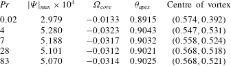
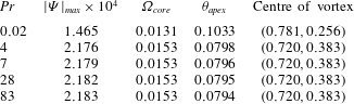
Streamfunction extremum, vorticity at the vortex core, apex temperature and coordinate of the centre of the vortex in Cartesian coordinates
 $(x,y)$
for different Prandtl numbers. The parameters are the same as in figure 8.
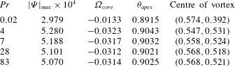
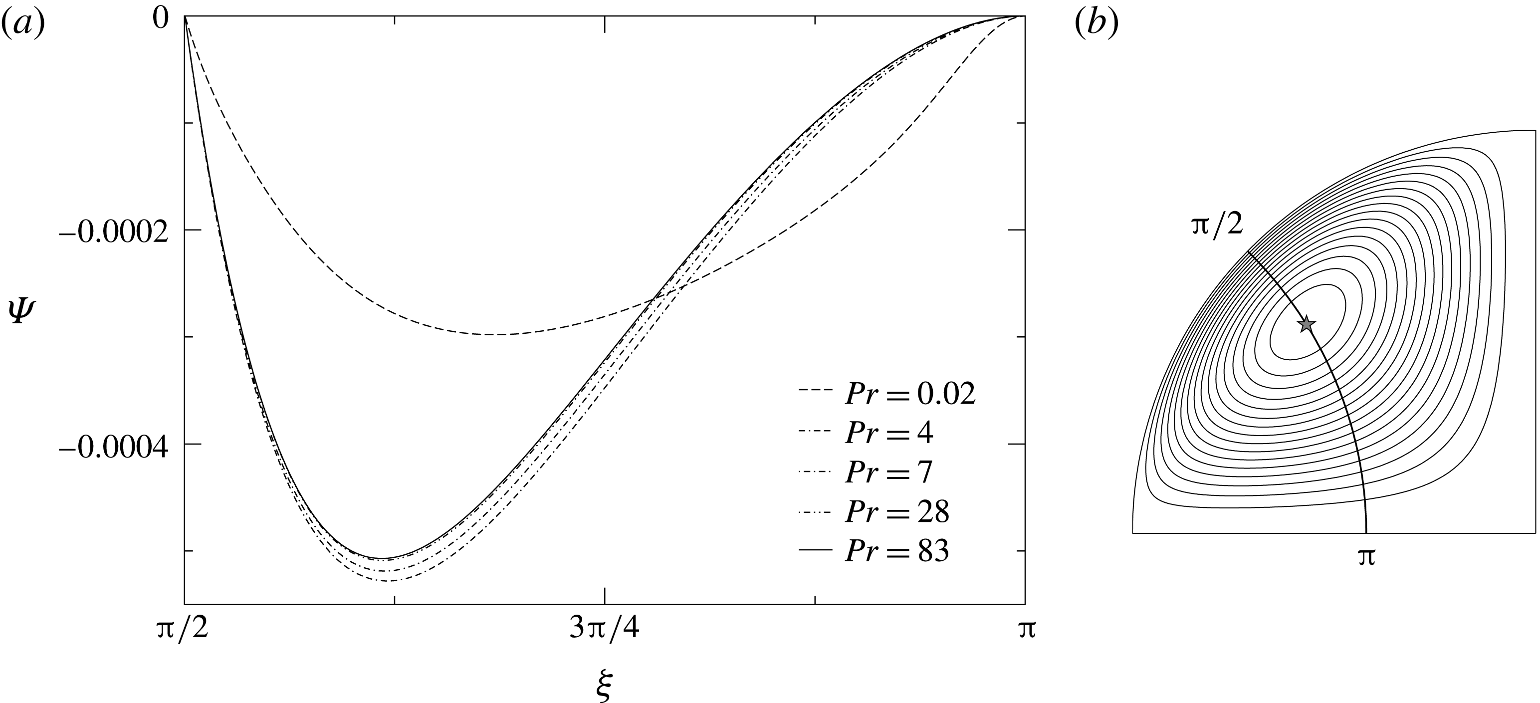
To characterise the structure of the toroidal vortex streamfunction profiles are shown in figure 8(a) for different Prandtl numbers considering
 $Ma=Re\,Pr=2800$
and keeping all other parameters constant. In the figure the streamfunction is displayed as a function of
 $\unicode[STIX]{x1D709}$
along the
 $\unicode[STIX]{x1D702}$
-coordinate which passes through the global maximum of
 $|\unicode[STIX]{x1D6F9}|$
(see figure 8
b). For the low Prandtl number
 $Pr=0.02$
the flow is inertial with
 $Re=140\,000$
. For the higher Prandtl numbers the Reynolds number is much smaller and the vortex structure is very similar in these cases. More quantitative data, including the coordinate of the vortex centre, temperature at the drop’s apex as well as the vorticity at the core of the vortex are presented in table 4 in order to provide a better comparison between different cases. The listed data confirm the different flow behaviour for low and high Prandtl numbers. Comparing the temperature at the apex shows a lower temperature for the low Prandtl number case than the others which means that the convective heat transport is more influential in case of higher Prandtl numbers for a constant Marangoni number.
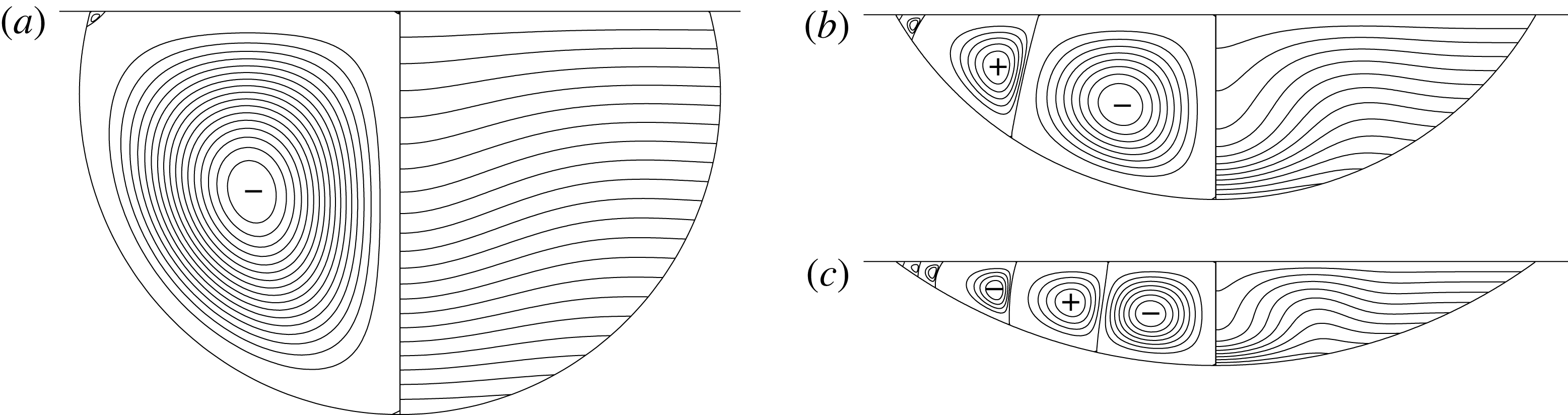
For all the cases considered in figure 8(a) (
 $Ma=\text{const.}$
) the temperature field is visually quite similar as illustrated in figure 9 for three selected cases. However, the streamlines of low and high Prandtl number cases are quite different. For the low Prandtl number case (figure 9
a) in which the flow is inertial, the centre of the vortex shifts away from the free surface. Furthermore, a flow separation is observed close to the contact line. In case of higher Prandtl numbers (figure 9
b,c) no visual difference can be observed comparing the streamlines and isotherms.
Constant Marangoni number,
 $Ma=2800$
for (a)
 $Pr=0.02$
, (b)
 $Pr=4$
and (c)
 $Pr=28$
.

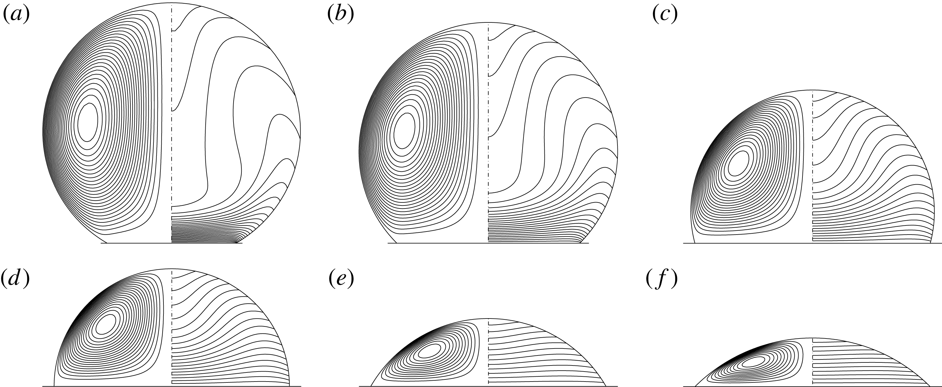
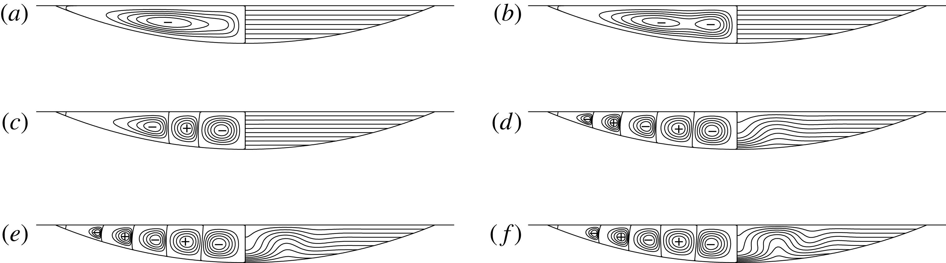
Streamlines and isotherms for different contact angles. The parameters are
 $Re=250$
,
 $Pr=4$
,
 $Gr=0$
and
 $Bi=0.1$
. (a)
 $\unicode[STIX]{x1D6FC}=150^{\circ }$
, (b)
 $\unicode[STIX]{x1D6FC}=120^{\circ }$
, (c)
 $\unicode[STIX]{x1D6FC}=105^{\circ }$
, (d)
 $\unicode[STIX]{x1D6FC}=90^{\circ }$
, (e)
 $\unicode[STIX]{x1D6FC}=60^{\circ }$
and (f)
 $\unicode[STIX]{x1D6FC}=45^{\circ }$
.

The contact angle is an important parameter for a droplet’s internal flow. Owing to the toroidal coordinates, droplets with a wide range of contact angles are easily realised by adjusting
 $\unicode[STIX]{x1D709}_{min}$
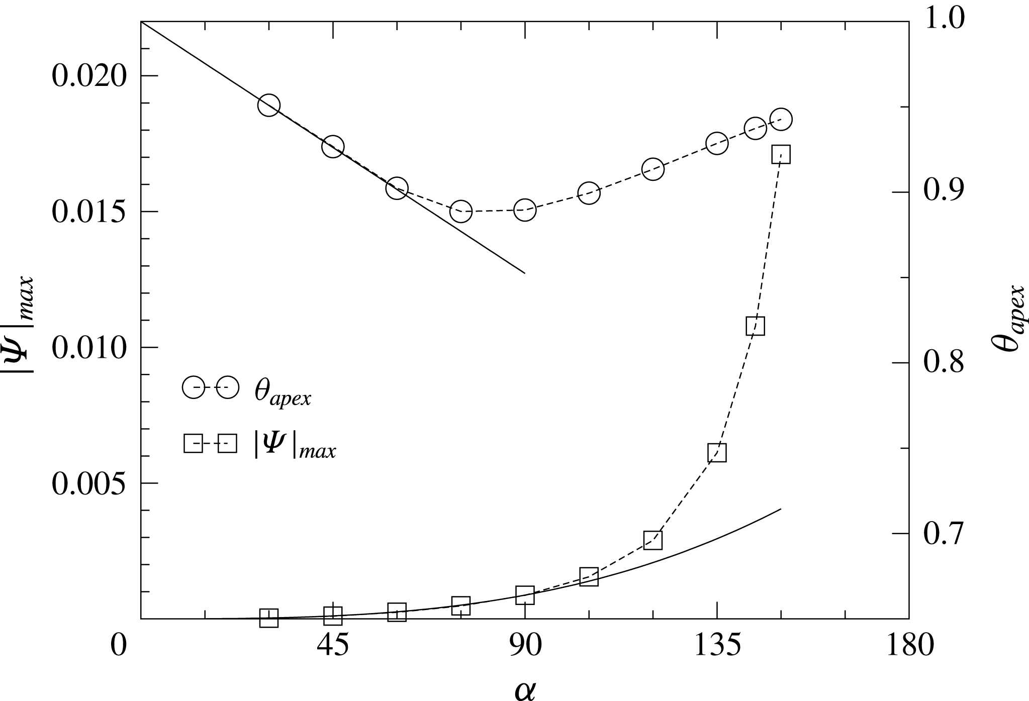
. Figure 10 shows streamlines as well as temperature isolines for a wide range of contact angles keeping the remaining parameters constant. In the asymptotic limit of shallow droplets the maximum thickness
 $l\sim \unicode[STIX]{x1D6FC}$
is proportional to the contact angle. An order of magnitude estimate of the heat-transfer boundary condition of (2.11d
) then shows that the effective driving temperature difference
 $1-\unicode[STIX]{x1D703}_{apex}\sim \unicode[STIX]{x1D6FC}$
scales linearly with the contact angle. Moreover, the balance between viscous and thermocapillary stresses in (2.11d
) yields a cubic scaling
 $\text{max}\,|\unicode[STIX]{x1D6F9}|\sim \unicode[STIX]{x1D6FC}^{3}$
of the streamfunction. Both scalings are confirmed by the numerical results for the given parameters shown in figure 11. For
 $Bi=0.1$
the effective temperature difference for the driving
 $1-\unicode[STIX]{x1D703}_{apex}$
takes a maximum value near
 $\unicode[STIX]{x1D6FC}=\unicode[STIX]{x03C0}/2$
which is approximately 10 % of the available temperature difference in the gas phase. For larger contact angles
 $1-\unicode[STIX]{x1D703}_{apex}$
shrinks. This effect is traced back to the enhanced convective heat transport from the wall to the apex, visible by the strong increase of the
 $\text{max}\,|\unicode[STIX]{x1D6F9}|$
. This enhanced convection for large contact angles is supported by the geometry (see also Kuhlmann, Nienhüser & Rath Reference Kuhlmann, Nienhüser and Rath1999; Nienhüser & Kuhlmann Reference Nienhüser and Kuhlmann2002): the highest surface stresses arise near the contact line on the hot wall. The larger the contact angle the less the flow is deflected near the contact line. As a result the flow acceleration is larger than for small contact angles which leads to an enhanced convective transport. This also leads to a crowding of isotherms near the contact line and thermal boundary layers begin to develop along the hot wall.
Streamfunction maximum
 $|\unicode[STIX]{x1D6F9}|_{max}$
(left axis, squares) and apex temperature
 $\unicode[STIX]{x1D703}_{apex}$
(right axis, circles) as functions of the contact angle
 $\unicode[STIX]{x1D6FC}$
. Parameters as in figure 10. Dotted lines are guides to the eye. The full lines represents the approximations
 $|\unicode[STIX]{x1D6F9}|_{max}=1.2\times 10^{-9}\unicode[STIX]{x1D6FC}^{3}$
and
 $\unicode[STIX]{x1D703}_{apex}=1{-}1.64\times 10^{-3}\unicode[STIX]{x1D6FC}$
.

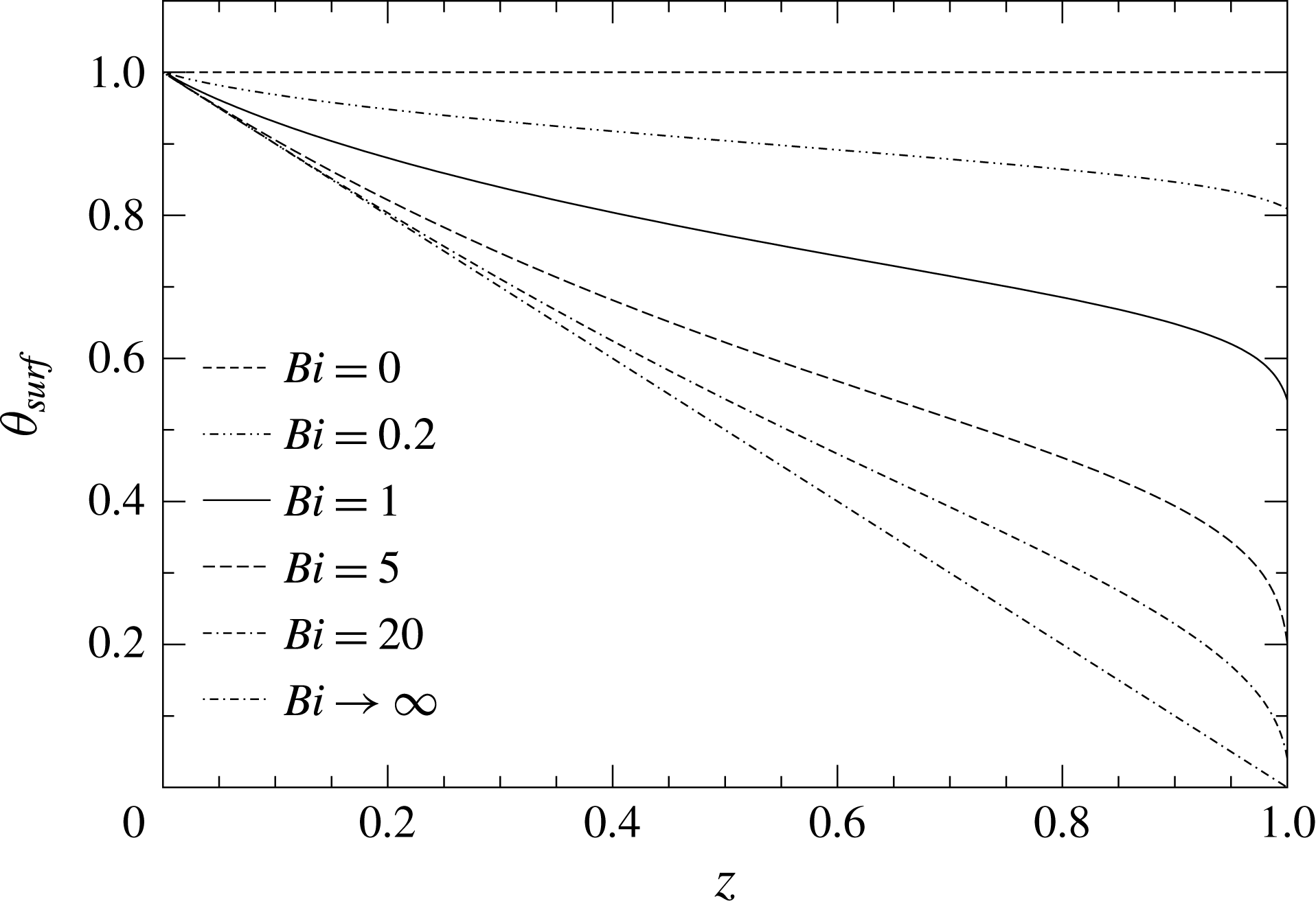
Another influential parameter on thermocapillary convection in the present setting is the Biot number. Figure 12 shows the temperature distribution on the free surface for different Biot numbers. For
 $Bi=0$
the free surface is adiabatic and the temperature is uniform along the free surface (and in the whole domain) corresponding to the wall temperature
 $\unicode[STIX]{x1D703}_{0}=1$
. In this case the fluid is at rest, since the thermocapillary driving forces vanish. In contrast, for large Biot numbers the surface temperature is nearly imposed by the ambient gas and the apex temperature of the droplet tends to
 $\unicode[STIX]{x1D703}_{apex}\rightarrow 0$
. The surface temperature distribution for
 $Bi=20$
is already close to the asymptotic case when
 $Bi\rightarrow \infty$
.
Temperature distribution along the free surface
 $\unicode[STIX]{x1D703}_{surf}$
as a function of the distance
 $z$
from the plate for different Biot numbers. The parameters are
 $Re=250$
,
 $Pr=4$
,
 $Gr=0$
and
 $\unicode[STIX]{x1D6FC}=\unicode[STIX]{x03C0}/2$
.

4.1.2 Buoyancy-driven flow
On small length scales thermocapillarity dominates buoyancy, since
 $Gr/Re\sim R^{2}$
vanishes as
 $R\rightarrow 0$
. Nevertheless, we investigate the effect of buoyancy for a large range of Grashof numbers
 $0<Gr<5000$
to better understand the combined thermocapillary–buoyant flow. For a sessile droplet on a hot plate, a thermal stratification for
 $\unicode[STIX]{x1D6FD}>0$
can be unstable, whereas for a pending droplet a thermal stratification is buoyantly stable. Therefore, we consider the more interesting the case of a sessile drop. In a first step we treat the purely buoyant flow and employ a viscous scaling in which
 $U^{\star }=\unicode[STIX]{x1D708}/R$
. The governing equations can then be obtained from (2.1) by setting
 $Re=1$
and by replacing the thermocapillary stress boundary condition (2.3) by a free-slip condition.
Isotherms for zero gravity and no thermocapillarity. The parameters are
 $Pr=28$
,
 $\unicode[STIX]{x1D6FC}=\unicode[STIX]{x03C0}/2$
and (a)
 $Bi=0.1$
, (b)
 $Bi=1$
, (c)
 $Bi=10$
, (d)
 $Bi=100$
, (e)
 $Bi=10^{5}$
.

In the formal limit
 $Bi\rightarrow \infty$
the surface temperature is imposed and the isotherms are horizontal in the state of rest. For such an unstable density stratification the onset of convection can be correlated by the Rayleigh number
 $Ra=GrPr$
. When the Rayleigh number exceeds the critical value
 $Ra_{c}\approx 3080\pm 50$
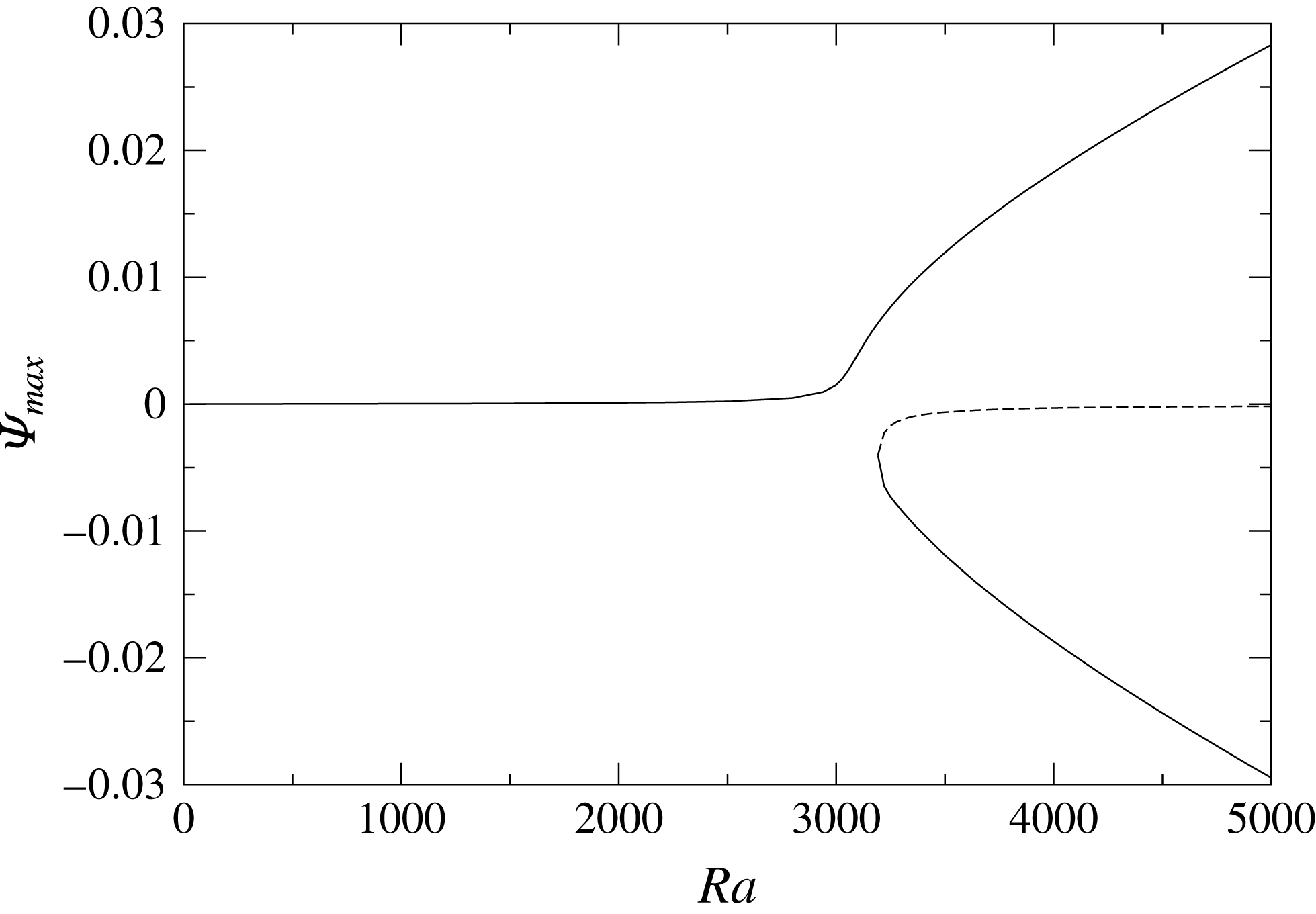
a flow arises in form of toroidal vortices. Owing to the symmetry of the linear stability equations two neutral solutions (two directions of rotation of the vortices) bifurcate from the basic state through a pitchfork bifurcation. For a finite Biot number, weak horizontal temperature gradients exist (for pure conduction see figure 13) which drive a weak flow for any non-zero Rayleigh number such that the bifurcation is perturbed. For a heated plate and contact angle
 $\unicode[STIX]{x1D6FC}=\unicode[STIX]{x03C0}/2$
the horizontal temperature gradient is directed radially inward, driving a toroidal vortex with up-flow on the axis. Apart from this favoured flow direction a stable and an unstable state with down-flow on the axis are created via a saddle-node bifurcation near
 $Ra=Ra_{c}(Bi\rightarrow \infty )$
. An example for the imperfect bifurcation is shown in figure 14 for
 $Bi=100$
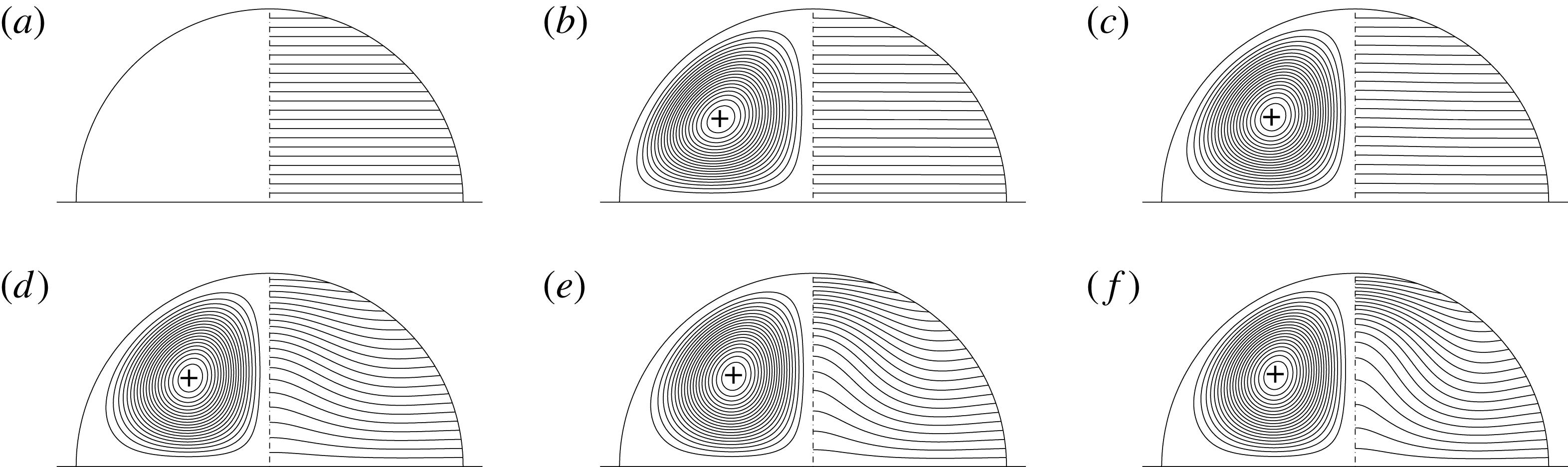
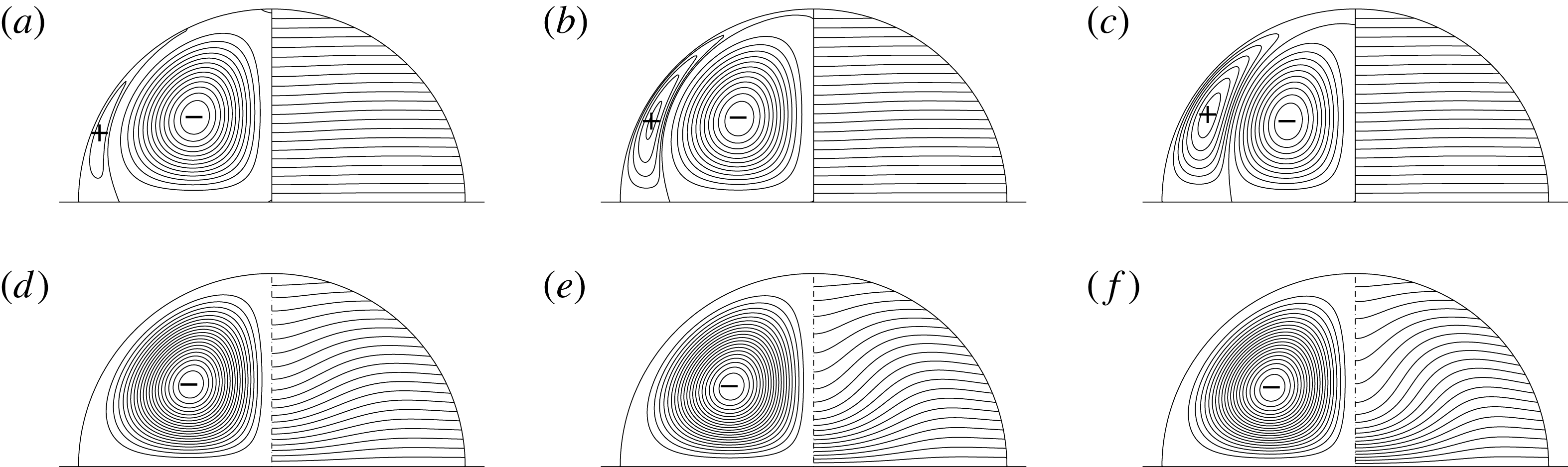
. Figures 15 and 16(d–f) show the streamlines and isotherms as a function of the Rayleigh number for the two different stable solutions with up- and down-flow on the axis, respectively. Moreover, the unstable solutions are shown in figure 16(a–c).
Perturbed pitchfork bifurcation showing the maximum of
 $\unicode[STIX]{x1D6F9}$
as a function of the Rayleigh number for
 $Bi=100$
.

Streamlines and isotherms for pure buoyant flow with up-flow on the axis (
 $+$
sign) corresponding to the upper full line in figure 14. The parameters are
 $Pr=28$
,
 $\unicode[STIX]{x1D6FC}=\unicode[STIX]{x03C0}/2$
,
 $Bi=100$
and (a)
 $Ra=0$
, (b)
 $Ra=1400$
, (c)
 $Ra=2800$
, (d)
 $Ra=3360$
, (e)
 $Ra=3920$
, (f)
 $Ra=4480$
.

Streamlines and isotherms for pure buoyant flow with down-flow on the axis. The unstable case (a–c): dashed line in figure 14 and second stable case (d–f): lower solid branch of the bifurcation diagram. The minus/plus sign (
 $\mp$
) indicates the clockwise/counterclockwise rotation. The parameters are
 $Pr=28$
,
 $\unicode[STIX]{x1D6FC}=\unicode[STIX]{x03C0}/2$
,
 $Bi=100$
and (a,d)
 $Ra=3360$
, (b,e)
 $Ra=3920$
, (c,f)
 $Ra=4480$
.

4.1.3 Thermocapillary–buoyant flow
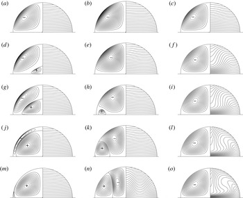
Figure 17 shows the evolution of the flow as a function of the Grashof number for
 $Pr=0.02$
(a,d,g,j,m),
 $Pr=4$
(b,e,h,k,n) and
 $Pr=83$
(c,f,i,l,o) when the Reynolds number is small. In the absence of buoyancy
 $(Gr=0)$
the thermocapillary flow drives a single toroidal vortex with down-flow on the centreline (
 $-$
). Depending on the temperature field of the thermocapillary flow at
 $Gr=0$
different thermocapillary–buoyant flow structures evolve upon an increase of
 $Gr$
.
Streamlines and isotherms for mixed buoyant–thermocapillary flow for
 $\unicode[STIX]{x1D6FC}=\unicode[STIX]{x03C0}/2$
,
 $Bi=0.5$
. (a,d,g,j,m)
 $Pr=0.02$
and
 $Re=25$
for
 $Gr=100,1300,1600,2400,3000$
(from top to bottom). (b,e,h,k,n)
 $Pr=4$
and
 $Re=10$
for
 $Gr=100,1000,1400,2000,4000$
. (c,f,i,l,o)
 $Pr=83$
and
 $Re=1$
for
 $Gr=10,100,200,500,1000$
.

For
 $Pr=0.02$
the Marangoni number is
 $Ma=0.5$
. Due to the minute convective effect the radial temperature distribution has a maximum at the centreline
 $r=0$
. As a result, a toroidal buoyantly driven vortex (
 $+$
) is created at
 $r=0$
on the bottom plate. As
 $Gr$
increases the buoyantly driven vortex increases in size and the thermocapillary driven vortex is squeezed to the free surface before it is completely suppressed by the buoyancy-driven vortex.
In the intermediate Prandtl number case (figure 17
b,e,h,k,n) the Marangoni number is
 $Ma=40$
and the maximum temperature at constant height
 $z$
arises at an intermediate radial distance. In this situation buoyancy forces augment the thermocapillary flow in the inner region near the axis, while buoyancy is opposing the thermocapillary flow in the radially outer region. This seems to be the reason why a buoyantly driven vortex
 $(+)$
is created on the bottom plate near the contact line. For the present parameters the buoyancy-driven vortex grows as
 $Gr$
increases and also occupies part of the free surface. Therefore, the thermocapillary-driven vortex is displaced toward the axis.
Finally, for the highest Prandtl number considered (figure 17
c,f,i,l,o), the Marangoni number
 $Ma=415$
is sufficiently large such that the convective deformation of the temperature field is much larger than the conductive part of the temperature field. The temperature maximum at constant height
 $z$
arises close to the free surface. Due to the high Rayleigh number buoyant forces are strongly augmenting the vortex with down-flow on the centreline, which amplifies the thermocapillary-driven vortex. Apparently, the radial temperature gradients in the outer region near the free surface are too weak to lead to a separated buoyantly driven vortex as for lower Prandtl numbers.
To provide quantitative data we consider
 $Pr=0.02$
and
 $Gr=3000$
and vary
 $Re$
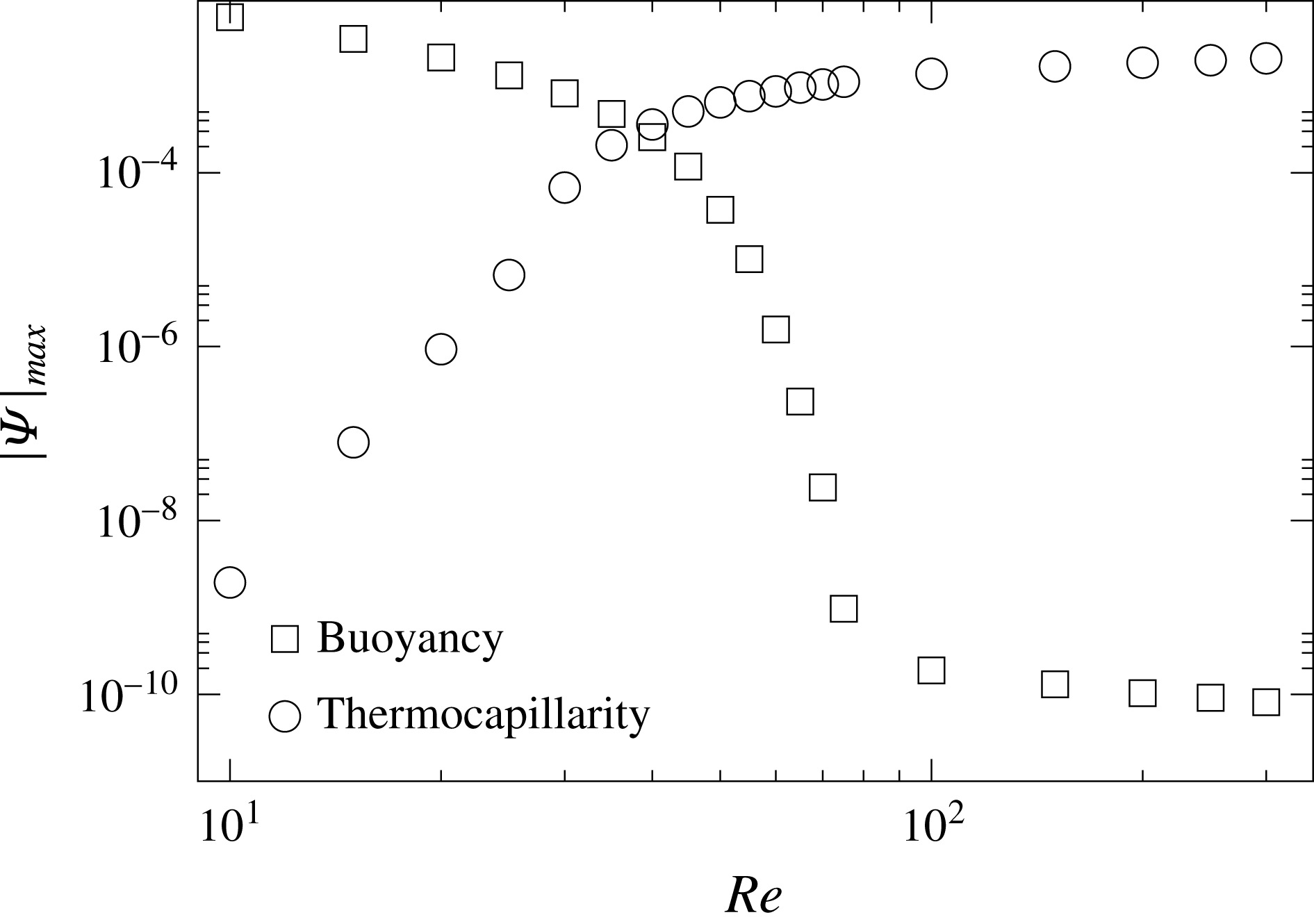
. The competition between the buoyancy- and thermocapillary-driven vortices is quantified in figure 18 by the values of the two extrema of different signs of the streamfunction. For small Reynolds numbers, the buoyant vortex dominates. By increasing
 $Re$
the thermocapillary forces become stronger and the thermocapillary vortex replaces the buoyant one. The cross-over when both streamfunction extrema have the same magnitude occurs at
 $Re\approx 40$
. As shown before, due to the increased convective effect on the temperature field the buoyancy-force field changes and a buoyancy-driven separated vortex may be completely suppressed.
Absolute values of the streamfunction extrema
 $|\unicode[STIX]{x1D6F9}|_{max}$
for the vortices driven by buoyancy
 $(\unicode[STIX]{x1D6F9}_{max}>0)$
and thermocapillarity
 $(\unicode[STIX]{x1D6F9}_{min}<0)$
as functions of the Reynolds number. The parameters are
 $Gr=3000$
,
 $Pr=0.02$
,
 $Bi=0.5$
and
 $\unicode[STIX]{x1D6FC}=\unicode[STIX]{x03C0}/2$
.

4.1.4 Latent heat of evaporation – homogeneous mass flux
If the droplet is not too small the relative rate of change of the droplet volume
 $\dot{V}/V$
due to evaporation is small in a gas which is quiescent far away from the droplet. Under such conditions the main effect of evaporation on the flow inside the droplet is caused by the latent heat. Therefore, the assumption of a quasi-steady evaporation process which does not affect the shape of the spherical-cap-shaped free surface is valid (Savino et al.
Reference Savino, Paterna and Favaloro2002). Since we do not solve the transport equations in the ambient gas the release of latent heat of evaporation has to be modelled. The modelling is facilitated by considering a contact angle
 $\unicode[STIX]{x1D6FC}=\unicode[STIX]{x03C0}/2$
for which the evaporative mass flux is nearly uniformly distributed over the liquid–gas interface (Stauber et al.
Reference Stauber, Wilson, Duffy and Sefiane2015). Under these conditions the total dimensional heat flux through the free surface due to evaporation can be written as
 $$\begin{eqnarray}\dot{Q}_{ev}=\unicode[STIX]{x1D70C}q_{ev}\dot{V},\end{eqnarray}$$
where
 $q_{ev}$
is the heat of vaporisation. Using the scales of table 1 the non-dimensional average heat-flux density through the free surface area
 $S$
becomes
 $$\begin{eqnarray}j=\unicode[STIX]{x1D70C}q_{ev}\frac{\dot{V}}{S}\frac{R}{k\unicode[STIX]{x0394}T}=\frac{q_{ev}\unicode[STIX]{x1D6FE}R^{3}}{3k\unicode[STIX]{x1D708}^{2}}\frac{\dot{V}}{V}\frac{1}{Re},\end{eqnarray}$$
where the time scale is arbitrary. In the second step we used
 $S=3V/R$
for a droplet with
 $\unicode[STIX]{x1D6FC}=\unicode[STIX]{x03C0}/2$
and expressed
 $\unicode[STIX]{x0394}T$
through
 $Re$
. For a radius of
 $R=2.5~\text{mm}$
and the material data of acetone (Simic-Stefani, Kawaji & Yoda Reference Simic-Stefani, Kawaji and Yoda2006) one obtains the estimate
 $j\approx 1.5\times 10^{7}~\text{s}^{-1}(\dot{V}/V)Re^{-1}$
. Together with the measured volume loss from millimetric liquid bridges of
 $\dot{V}/V(R=2.5~\text{mm})=2\times 10^{-4}\cdots 10^{-3}~\text{s}^{-1}$
(Simic-Stefani et al.
Reference Simic-Stefani, Kawaji and Yoda2006) and
 $Re=O(10^{3})$
the heat current density is of order one in our scaling.
Influence of the latent heat of vaporisation on flow and temperature fields for (a)
 $j=0.1$
, (b)
 $j=0.25$
and (c)
 $j=1$
. The parameters are
 $Re=1000$
,
 $Pr=4$
,
 $Bi=0.1$
,
 $Gr=0$
and
 $\unicode[STIX]{x1D6FC}=\unicode[STIX]{x03C0}/2$
.

To take into account the effect of evaporation the average heat-flux density due to the latent heat of evaporation is added to Newton’s heat-flux density to obtain the modified heat-transfer boundary condition
 $$\begin{eqnarray}\unicode[STIX]{x2202}_{\unicode[STIX]{x1D709}}\unicode[STIX]{x1D703}=j+Bi(\unicode[STIX]{x1D703}-\unicode[STIX]{x1D703}_{a}).\end{eqnarray}$$
Figure 19 shows the flow and temperature fields in a sessile droplet for three different values of the latent-heat flux (
 $j=0.1,0.25,$
and
 $1$
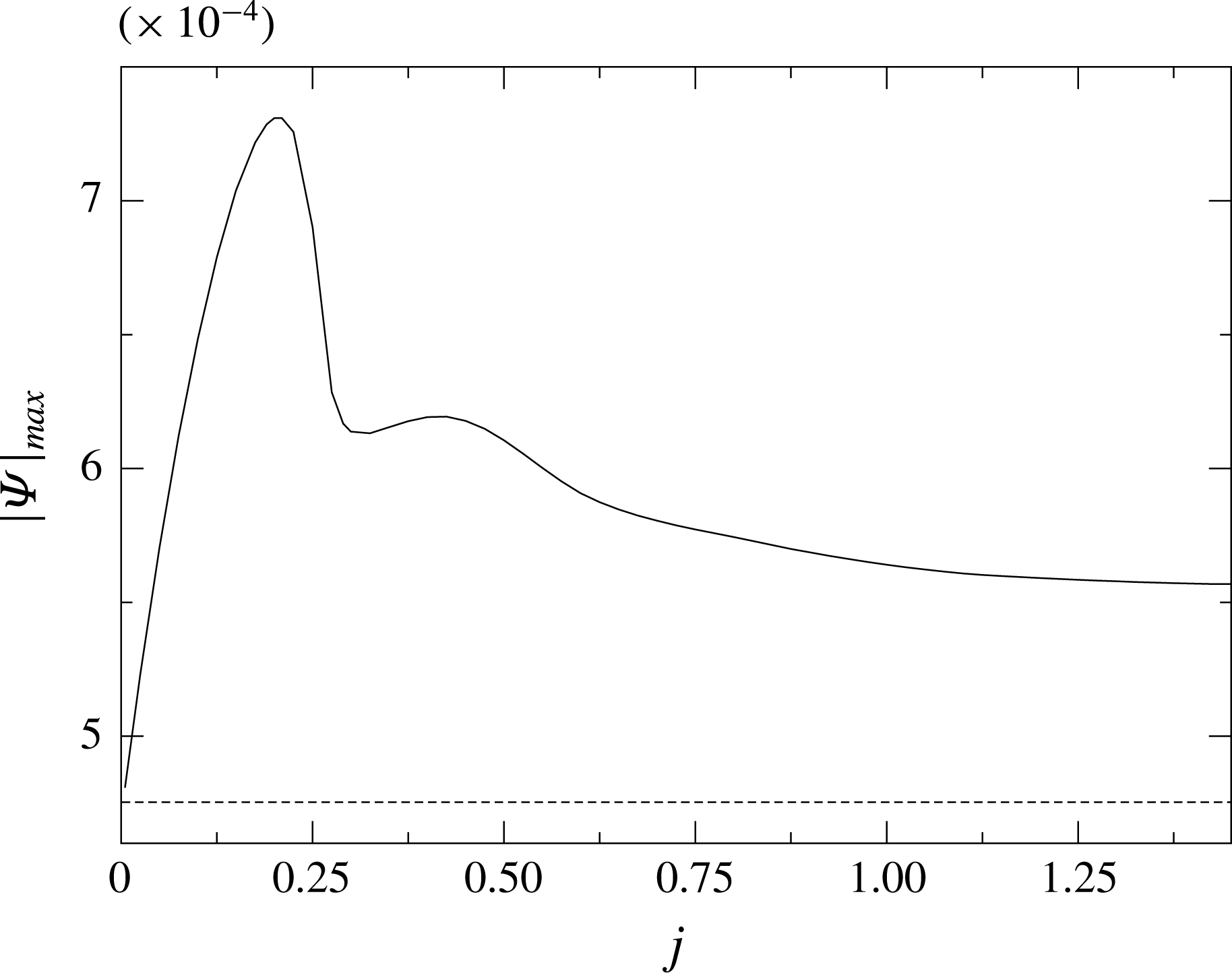
). The flow pattern is not very much influenced by the latent-heat effect in this range. The strength of the flow,
 $|\unicode[STIX]{x1D6F9}|_{max}$
, exhibits two local maxima by varying the latent heat of evaporation as shown in figure 20. However, the variation of
 $|\unicode[STIX]{x1D6F9}|_{max}(j)$
with
 $j$
is significantly less than the value
 $|\unicode[STIX]{x1D6F9}|_{max}(0)$
in the absence of evaporation (dashed line in figure 20).
Absolute value of the streamfunction extrema
 $|\unicode[STIX]{x1D6F9}|_{max}$
as a function of the heat flux due to latent heat. The parameters are the same as in figure 19. The dashed line is to ease the comparison of the plotted values with the case in which the latent heat is neglected.

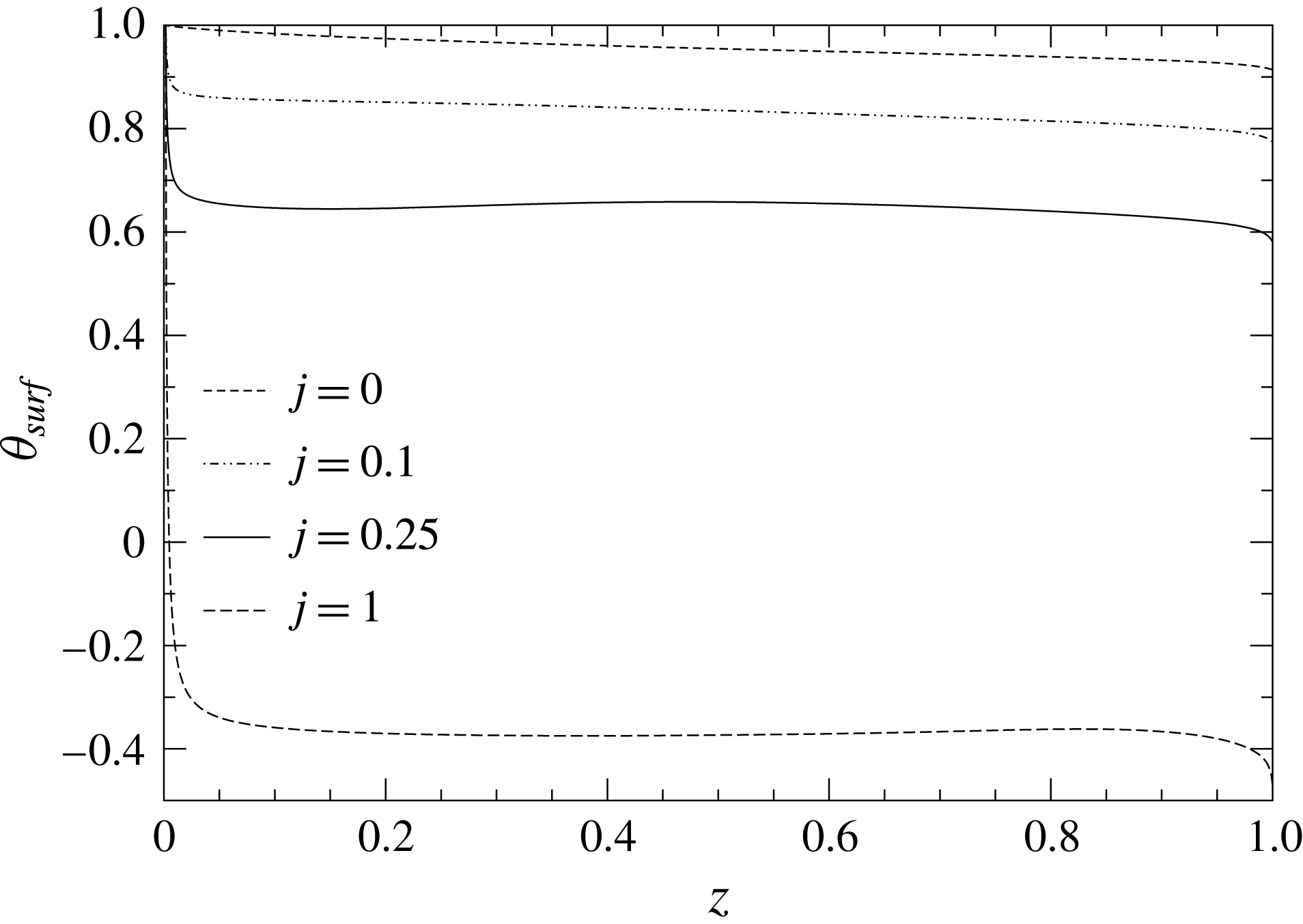
A comparison between the evaporative cases shown in figure 19 is provided in figure 21 by displaying surface temperature profiles. In all cases the surface temperature does not vary much except for a small region near the contact line. This observation is consistent with the approximation of homogeneously distributing the total heat flux over the entire surface in (4.3). The mean surface temperature of the droplet is strongly reduced as the evaporation effect becomes more intense. For
 $j=1$
the free surface temperature even drops below the minimum ambient temperature at the apex level of the sessile droplet. In the absence of evaporation the flow is driven all along the free surface (short-dashed line in figure 21). Since the evaporative cooling reduces the interfacial temperature, large temperature gradients are created near the contact line which enhance the flow (see figure 20 for
 $j<0.2$
). As the evaporative cooling becomes stronger a temperature plateau with a weak maximum develops at midheight levels which reduces the diving force over most part of the interface except for the corner region. This causes the first maximum of
 $|\unicode[STIX]{x1D6F9}|_{max}$
in figure 20. Apparently, the strongly localised temperature gradient near the contact line is not able to further increases the intensity of the flow as
 $j$
is increased beyond
 $j=0.5$
.
Temperature distribution along the free surface
 $\unicode[STIX]{x1D703}_{surf}$
as a function of the distance
 $z$
from the plate for different values of
 $j$
. The parameters are
 $Re=1000$
,
 $Pr=4$
,
 $Gr=0$
,
 $Bi=0.1$
and
 $\unicode[STIX]{x1D6FC}=\unicode[STIX]{x03C0}/2$
.

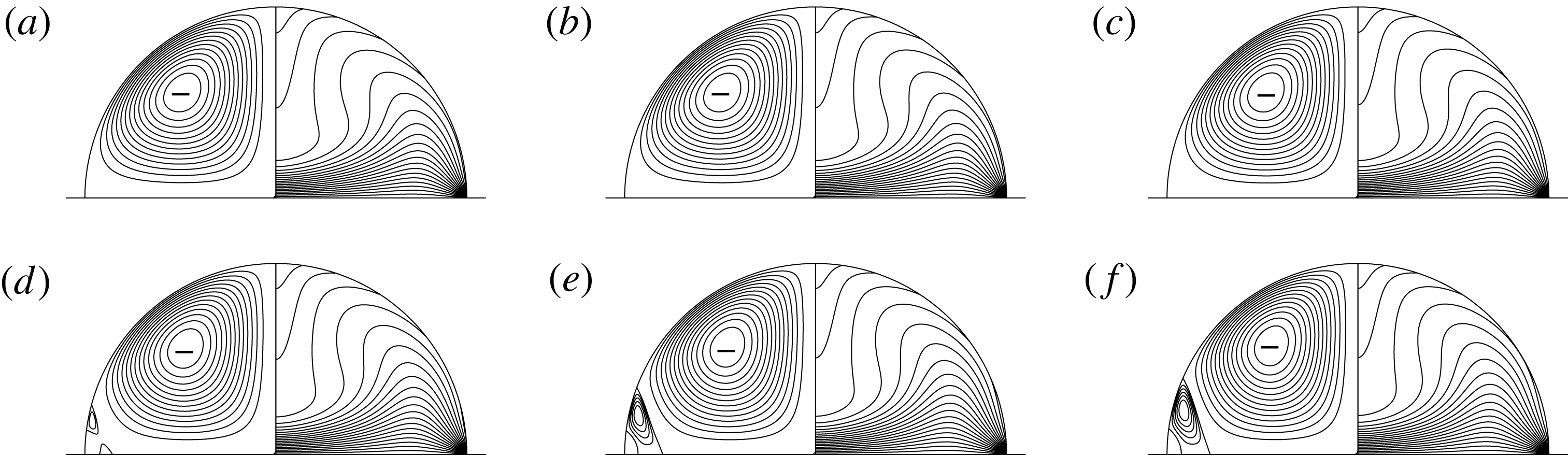
An example for the combined effect of buoyancy, thermocapillarity and evaporation is shown figure 22 for
 $j=0.25$
. As the buoyancy level is increased the isotherm pattern does not change qualitatively. However, due to the increased surface forces as a result of evaporation the flow separates near the contact line as the Grashof number is increased. Initially, we find two small distinguished separation zones, one on the free surface and another one on the hot wall (figure 22
d). For larger Grashof numbers both separation zones merge and result in two small counter-rotating toroidal vortices near the contact line (figure 22
e). A similar flow structure has been observed experimentally by Al-Sharafi et al. (Reference Al-Sharafi, Ali, Yilbas, Sahin, Khaled, Al-Aqeeli and Al-Sulaiman2016) for droplets of large contact angles sitting on hydrophobic surfaces. They reported a pair of counter-rotating circulation cells in a sessile droplet.
Variation of the gravity level for
 $Re=1000$
,
 $Pr=4$
,
 $j=0.25$
and
 $Bi=0.1$
. (a)
 $Gr=25$
, (b)
 $Gr=100$
, (c)
 $Gr=500$
, (d)
 $Gr=800$
, (e)
 $Gr=1000$
and (f)
 $Gr=1050$
.

4.1.5 Latent heat of evaporation – inhomogeneous mass flux
To investigate evaporating droplets for contact angles other than
 $90^{\circ }$
, the non-uniformity of the evaporation mass flux over the liquid–gas interface has to be taken into account. Since the transport equations in the ambient gas are not solved in the present approach, we use the analytical expressions for the local evaporation mass flux developed by Deegan et al. (Reference Deegan, Bakajin, Dupont, Huber, Nagel and Witten2000) and Hu & Larson (Reference Hu and Larson2002). Their correlations very accurately approximate the solution of the stationary diffusion equation in the ambient gas when the Stefan flow is neglected. Defining the dimensionless evaporation number
 $$\begin{eqnarray}E=\frac{\unicode[STIX]{x1D70C}\unicode[STIX]{x1D708}q_{ev}}{k\unicode[STIX]{x0394}T},\end{eqnarray}$$
the heat-transfer boundary condition between the droplet and the ambient gas can be written as
 $$\begin{eqnarray}\unicode[STIX]{x2202}_{\unicode[STIX]{x1D709}}\unicode[STIX]{x1D703}=EJ_{0}(\unicode[STIX]{x1D6FC})+Bi(\unicode[STIX]{x1D703}-\unicode[STIX]{x1D703}_{a}),\end{eqnarray}$$
where
 $J_{0}(\unicode[STIX]{x1D6FC})$
is the evaporation mass flux at the surface of the droplet. According to Hu & Larson (Reference Hu and Larson2002)
 $J_{0}(\unicode[STIX]{x1D6FC})$
can be modelled as
 $$\begin{eqnarray}J_{0}(\unicode[STIX]{x1D6FC})=J_{0}\left(\frac{\unicode[STIX]{x03C0}}{2}\right)\left[0.6381-0.2239\left(\unicode[STIX]{x1D6FC}-\frac{\unicode[STIX]{x03C0}}{4}\right)^{2}\right](0.27\unicode[STIX]{x1D6FC}^{2}+1.3)\left[1-\left(\frac{r}{R}\right)^{2}\right]^{-0.5+\unicode[STIX]{x1D6FC}/\unicode[STIX]{x03C0}},\end{eqnarray}$$
in which
 $J_{0}(\unicode[STIX]{x03C0}/2)$
represents the uniform evaporation mass flux the effect of which was discussed in the previous subsection. The evaporation mass flux, diffusively scaled with
 $\unicode[STIX]{x1D70C}\unicode[STIX]{x1D708}/R$
, can be written as (Hu & Larson Reference Hu and Larson2002)
 $$\begin{eqnarray}J_{0}\left(\frac{\unicode[STIX]{x03C0}}{2}\right)=\frac{D(1-H)c_{v}}{\unicode[STIX]{x1D70C}\unicode[STIX]{x1D708}},\end{eqnarray}$$
where
 $D$
is the vapour diffusivity,
 $c_{v}$
the saturated vapour concentration and
 $H$
the relative humidity in the ambient gas. The remainder of the right-hand side of (4.6) depends only on the contact angle and the relative radial distance of the surface point from the axis which can be written as
 $r/R=\sinh \unicode[STIX]{x1D702}[\cosh \unicode[STIX]{x1D702}-\cos \unicode[STIX]{x1D709}]^{-1}$
.
In order to solve the problem numerically, we consider acetone with
 $\unicode[STIX]{x1D70C}=791~\text{kg}~\text{m}^{-3}$
,
 $\unicode[STIX]{x1D708}=4\times 10^{-7}~\text{m}^{2}~\text{s}^{-1}$
,
 $k=0.165~\text{W}~(\text{m}~\text{K})^{-1}$
,
 $c_{v}=563~\text{g}~\text{m}^{-3}$
,
 $D=0.103~\text{cm}^{2}~\text{s}^{-1}$
and assume
 $H=0.9$
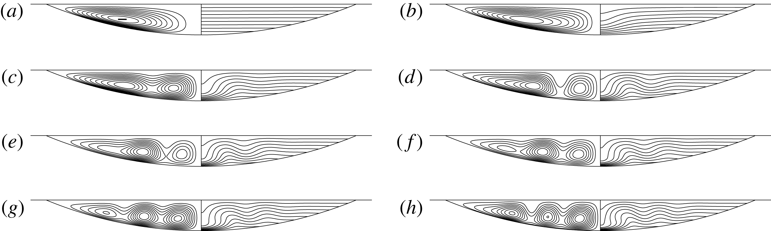
. Figure 23 illustrates the flow and temperature fields of droplets with different contact angles (
 $\unicode[STIX]{x1D6FC}<90^{\circ }$
) considering uniform (a,c,e,g) and non-uniform (b,d,f,h) evaporation mass flux for
 $Re=1000$
,
 $Pr=4$
,
 $Bi=0.1$
and
 $Gr=0$
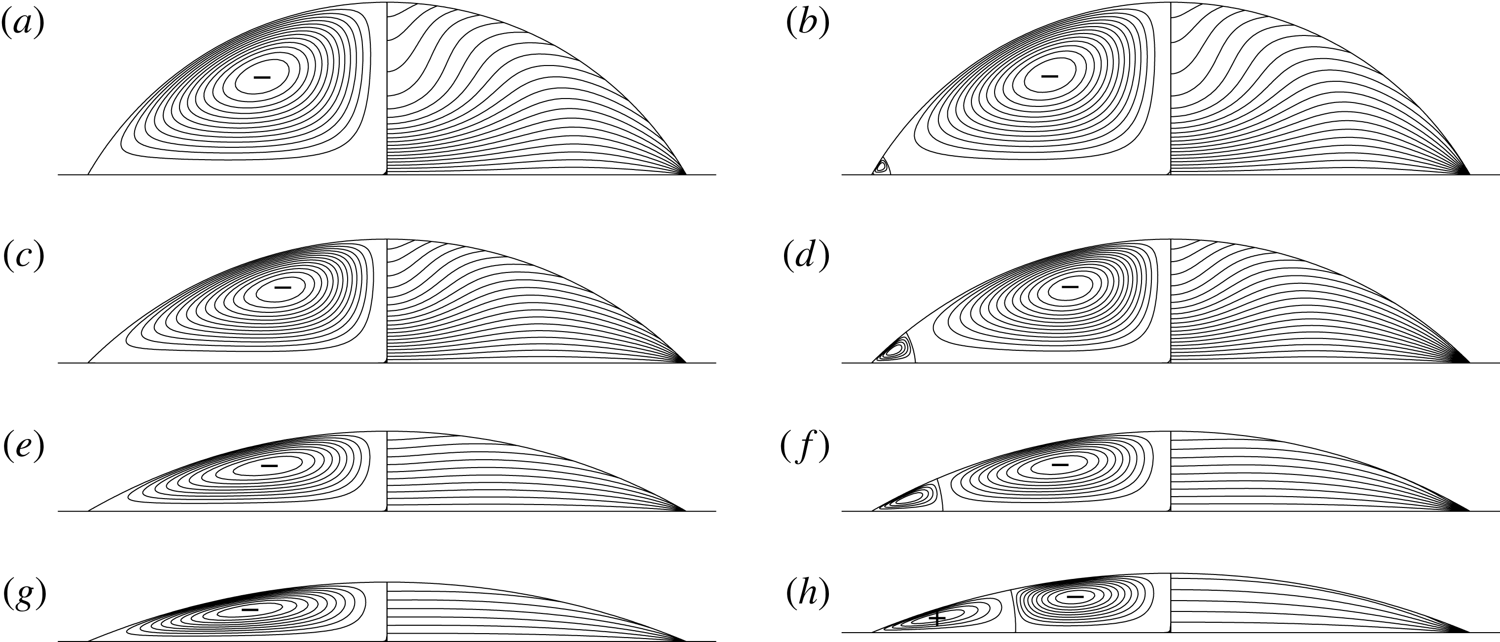
. In case of a non-uniform evaporation mass flux a minimum of the surface temperature arises close to the contact line, since the mass flux and evaporative cooling are strongest there. As a result, a single counter-rotating vortex (driven by thermocapillarity) is generated close to the contact line for all droplet shapes. The corner vortex is stronger (in terms of the streamfunction extremum) and extends over a larger radial distance the smaller the contact angle is, as the evaporation flux becomes stronger for shallower droplets (see Stauber et al.
Reference Stauber, Wilson, Duffy and Sefiane2015). Therefore, it can be concluded that the inhomogeneity of the evaporation mass flux has a strong effect on the flow for shallow droplets (
 $\unicode[STIX]{x1D6FC}<90^{\circ }$
). In particular, it is responsible for a strong corner vortex for which the surface velocity is directed towards the contact line.
Streamfunction and temperature fields for an evaporating acetone droplet for different contact angles (from a–h:
 $60^{\circ }$
,
 $45^{\circ }$
,
 $30^{\circ }$
,
 $22.5^{\circ }$
) and
 $Re=1000$
,
 $Pr=4$
,
 $Bi=0.1$
and
 $Gr=0$
. (a,c,e,g) Shows results for a homogeneous evaporation with
 $EJ_{0}(\unicode[STIX]{x03C0}/2)=0.47$
, (b,d,f,h) for an inhomogeneous evaporation according to (4.6).

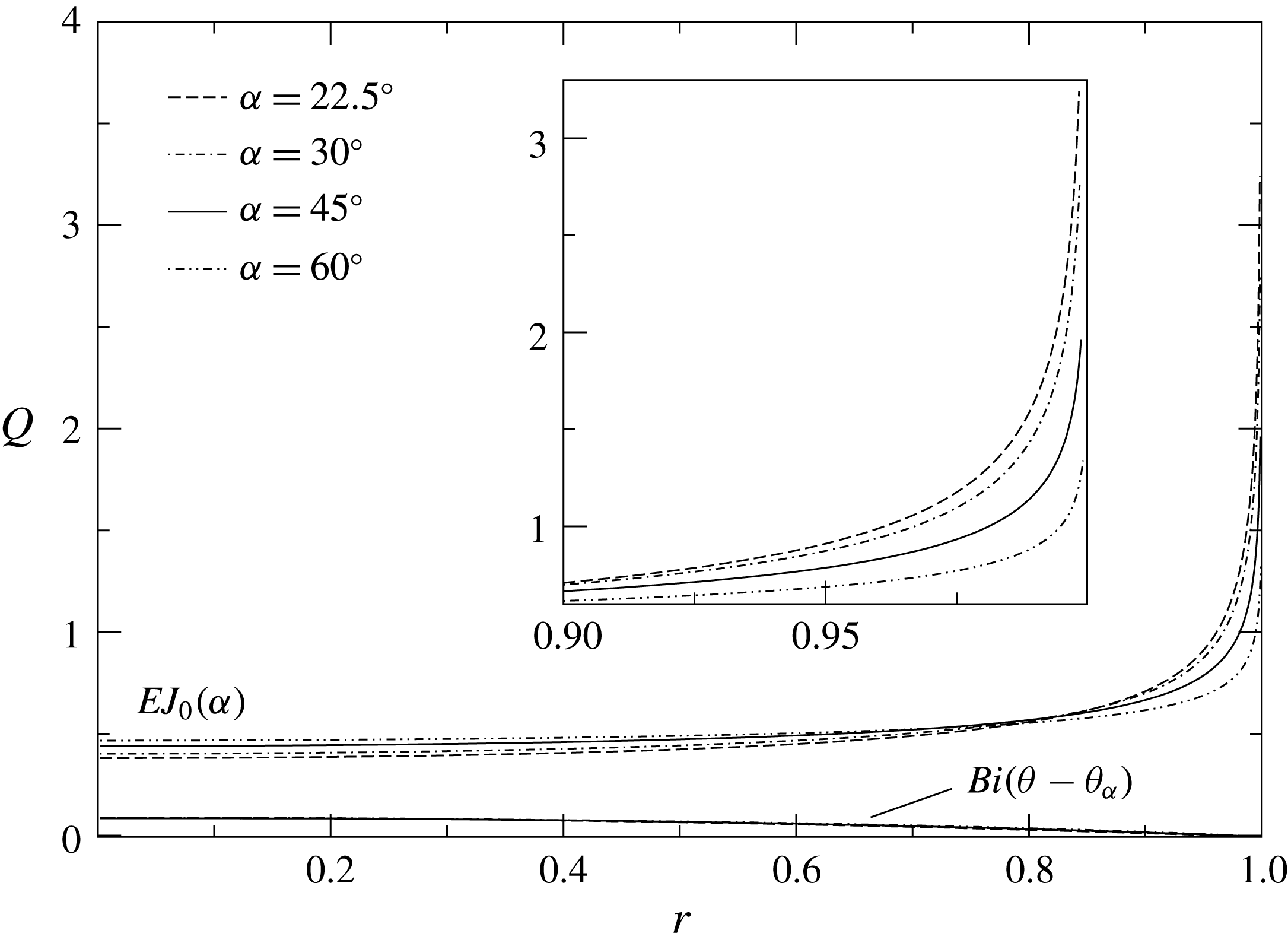
Figure 24 shows the two contributions to the heat-flux density at the liquid–gas interface due to evaporation
 $(EJ_{0}(\unicode[STIX]{x1D6FC}))$
and due to Newton’s heat transfer
 $(Bi(\unicode[STIX]{x1D703}-\unicode[STIX]{x1D703}_{a}))$
, both as functions of the radial distance from the axis. The parameters are the same as in figure 23(b,d,f,h). Owing to the high volatility of acetone the heat flux due to evaporation dominates. While the heat flux due to evaporation does not vary much over most part of the interface, it becomes very strong as the contact line is approached. This effect is more pronounced the smaller the contact angle is (Cazabat & Guena Reference Cazabat and Guena2010; Erbil Reference Erbil2012; Stauber et al.
Reference Stauber, Wilson, Duffy and Sefiane2015). On the contrary, the heat flux due to Newton’s heat transfer diminishes towards the contact line. This result underlines that the heat transfer due to evaporation becomes dominant near the contact line when the liquid is volatile and the droplet is very shallow.
Heat flux density
 $Q$
through the liquid–gas interface due to evaporation (
 $EJ_{0}(\unicode[STIX]{x1D6FC})$
) and Newton’s law (
 $Bi(\unicode[STIX]{x1D703}-\unicode[STIX]{x1D703}_{a})$
) as a function of radial distance from the droplets centre for the cases shown in figure 23(b,d,f,h).

4.2 Cooled plate
4.2.1 Thermocapillary flow
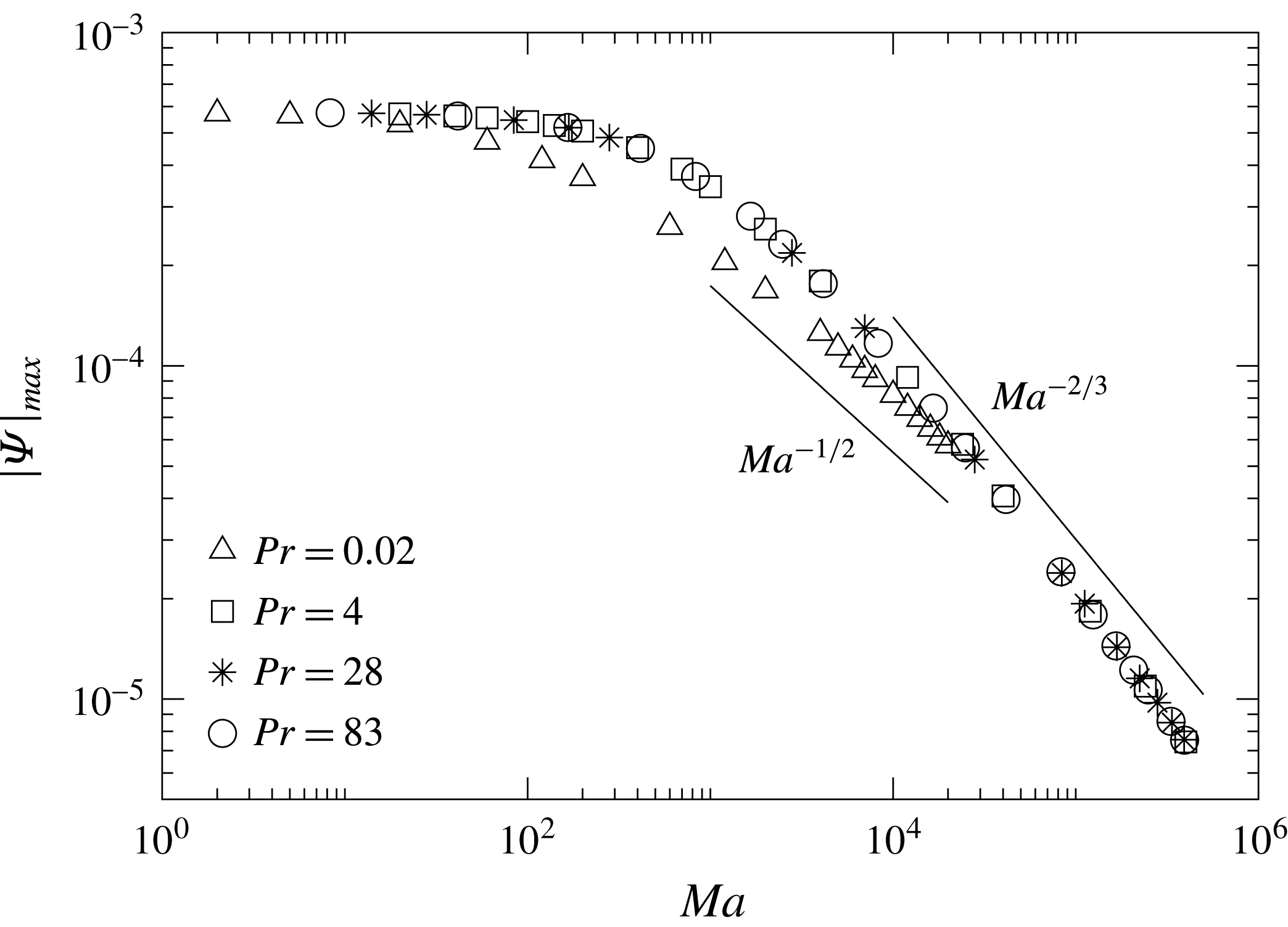
In the case of a cooled plate in a hot ambient, the thermocapillary flow is reversed, i.e. it is directed from the apex of the droplet toward the contact line along the free surface. The flow structure is illustrated in figure 25 for different parameters. As the Marangoni number increases the vortex centre arises closer to the contact line. For a more quantitative comparison, table 5 lists the apex temperature as well as
 $|\unicode[STIX]{x1D6F9}|_{max}$
for the cases presented in figure 25. Unlike the case of a heated plate in which
 $|\unicode[STIX]{x1D6F9}|_{max}$
as a function of Marangoni number exhibits a weak maximum (see figure 7) it decreases monotonically for all Prandtl numbers considered for the cooled plate as shown in figure 26. For low Prandtl numbers
 $(Pr=0.02)$
the streamfunction extremum scales like
 $\text{max}\,|\unicode[STIX]{x1D6F9}|\sim Ma^{-1/2}$
for
 $Ma>10^{3}$
, as for the case of a heated plate. For all the higher Prandtl numbers the strength of the flow scales with
 $\text{max}\,|\unicode[STIX]{x1D6F9}|\sim Ma^{-2/3}$
as the Marangoni number increases. The stronger decay of the streamfunction as compared to the case of a heated plate can be explained considering the temperature distribution within the droplet: by increasing the Reynolds number, the temperature along the free surface becomes almost constant (figure 25
i), except very close to the contact line where a large temperature gradient appears. The reduction of the length over which the thermocapillary stresses act leads to a reduced net driving of the flow.
Reynolds number variation for
 $Pr=0.02$
(a,d,g),
 $Pr=4$
(b,e,h) and
 $Pr=28$
(c,f,i), for
 $Gr=0$
and
 $Bi=0.1$
. (a–c)
 $Re=100$
, (d–f)
 $Re=250$
, (g–i)
 $Re=1000$
. For each droplet: streamlines (left quadrant) and isotherms (right quadrant).

Temperature at the droplets’ apex and
 $|\unicode[STIX]{x1D6F9}|_{max}$
for the cases shown in figure 25.

Maximum of
 $|\unicode[STIX]{x1D6F9}|$
as a function of
 $Ma$
.

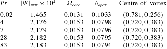
Table 6 lists some reference data for different Prandtl numbers when the Marangoni number is constant,
 $Ma=2800$
. Similar to the heated plate case (see table 4), there is a clear difference between the flow behaviour for low and high Prandtl numbers. However, unlike the heated plate case, for
 $Pr>1$
the characteristics of the flow remain almost unchanged. As it is explained before, in this case the temperature distribution is very similar which leads to the identical driving force within the flow field. This similar fluid flow is confirmed for a wide range of Marangoni numbers in figure 25.
Streamfunction extremum, vorticity at the vortex core, apex temperature and coordinate of the centre of the vortex in Cartesian coordinates
 $(x,y)$
for different Prandtl numbers. The parameters are
 $Ma=2800$
,
 $Bi=0.1$
,
 $Gr=0$
and
 $\unicode[STIX]{x1D6FC}=\unicode[STIX]{x03C0}/2$
.
4.2.2 Buoyant flow: influence of the contact angle
The temperature distribution in a droplet hanging from a cooled wall in a hot environment can be unstable for
 $\unicode[STIX]{x1D6FD}>0$
. The pure buoyant flow is calculated as for the heated plate case in the limit
 $Bi\rightarrow \infty$
. We find the same pitchfork bifurcation as in figure 14, as it should be due to the invariance with respect to
 $(g,\unicode[STIX]{x0394}T)\rightarrow (-g,-\unicode[STIX]{x0394}T)$
for
 $Re=0$
of the linearised equations and boundary conditions for perturbations of the conductive state. Therefore, we do not need to consider
 $\unicode[STIX]{x1D6FC}=\unicode[STIX]{x03C0}/2$
as in § 4.1.2. Instead, the dependence on the contact angle of pure buoyancy-driven flow in hanging droplets is considered. In the asymptotic limit of dominating surface tension the Rayleigh–Taylor instability is suppressed.
Pure buoyant flow in a shallow hanging droplet; gravity level variation for
 $Pr=28$
,
 $\unicode[STIX]{x1D6FC}=22.5^{\circ }$
and
 $Bi=100$
. (a)
 $Ra=280$
, (b)
 $Ra=980$
, (c)
 $Ra=1680$
, (d)
 $Ra=2240$
, (e)
 $Ra=2800$
and (f)
 $Ra=3360$
. For each droplet: streamlines (left quadrants) and isotherms (right quadrants).

Pure buoyant flow in hanging droplets of different contact angles. (a)
 $\unicode[STIX]{x1D6FC}=105^{\circ }$
, (b)
 $\unicode[STIX]{x1D6FC}=60^{\circ }$
and (c)
 $\unicode[STIX]{x1D6FC}=36^{\circ }$
. Parameters are
 $Ra=3360$
,
 $Pr=28$
and
 $Bi=100$
.

Figure 27 shows a shallow droplet for contact angle
 $\unicode[STIX]{x1D6FC}=22.5^{\circ }$
. For the low Rayleigh numbers
 $Ra=280$
the flow arises as a single-cell flow. Also for
 $Ra=980$
the flow is characterised by a global circulation, except for a weak cat’s eye structure. These flows are presumably due to the imperfect nature of the bifurcation at bounded Biot numbers. For
 $Ra=1680$
and larger, however, distinct but weak convective cells arise due to a thermal instability. The existence of weak convection cells in the shallow droplet at
 $Ra=1680$
is compatible, at least in order of magnitude, with the linear stability threshold
 $Ra_{c}=1100.65$
for a plane layer with mixed free and rigid boundary conditions at
 $k_{c}=2.682$
(Chandrasekhar Reference Chandrasekhar1961) and also compares favourably with the results of Vrentas, Narayanan & Agrawal (Reference Vrentas, Narayanan and Agrawal1981) for the onset of axisymmetric convection of high Prandtl number liquids in circular cylinders. As the Rayleigh number increases to
 $Ra=2240$
and beyond additional toroidal convection cells are created (figure 27
d). These eddies are generated, because the conductive state becomes locally unstable in the tapered region. In addition, viscous eddies may be driven by the stronger ones (Moffatt Reference Moffatt1964). Additional buoyancy-driven flow patterns for larger contact angles are shown in figure 28.
4.2.3 Thermocapillary–buoyant flow in a hanging droplet
For the combined thermocapillary–buoyant flow we consider only
 $Pr=83$
and
 $\unicode[STIX]{x1D6FC}=\unicode[STIX]{x03C0}/2$
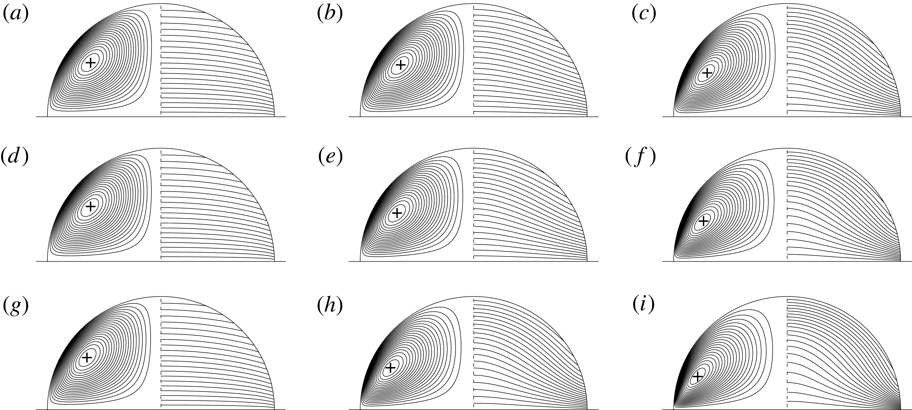
. The results for other Prandtl numbers are similar. Figure 29 shows a case of weak thermocapillarity with
 $Re=5$
. As buoyancy increases the single vortex flow becomes stronger, but the flow pattern does not change much. The reason is the buoyancy forces augmenting the thermocapillary flow. Thus no competition between the buoyant and thermocapillary forces arises as is the case of sessile droplets on a heated plate (figure 17).
Hanging droplet from a cooled plate. Streamlines and isotherms for mixed buoyant–thermocapillary flow;
 $Re=5$
,
 $Pr=83$
,
 $Bi=0.5$
, (a)
 $Gr=0$
; (b)
 $Gr=1000$
; (c)
 $Gr=3000$
.

The combined thermocapillary buoyant flow is more interesting for shallow hanging droplets. To enable a comparison with the pure buoyant flow, we consider similar parameters as in figure 27. For the moderate Reynolds number
 $Re=20$
shown in figure 30 the cellular flow is replaced by a multi-roll structure of co-rotating vortices with a global circulation. We find this multi-roll structure only in a narrow range of Reynolds numbers and for shallow droplets, when the Biot number is quite large. For droplets with larger contact angles, the thermocapillarity dominates the flow leading to a single-vortex flow.
Mixed buoyant–thermocapillary flow in a shallow hanging droplet; gravity level variation for
 $Re=20$
,
 $Pr=28$
,
 $Bi=100$
and
 $\unicode[STIX]{x1D6FC}=22.5^{\circ }$
. (a)
 $Ra=0$
, (b)
 $Ra=1120$
, (c)
 $Ra=1960$
, (d)
 $Ra=2240$
, (e)
 $Ra=2800$
, (f)
 $Ra=3360$
, (g)
 $Ra=3920$
and (h)
 $Ra=4480$
. For each droplet: streamlines (left quadrant) and isotherms (right quadrant).

5 Summary and conclusions
The steady two-dimensional incompressible axisymmetric flow in a wall-bounded droplet has been calculated numerically using body-fitted toroidal coordinates in the limit of dominating mean surface tension. The liquid droplet is either sitting on or hanging from an isothermal perfectly conducting flat horizontal plate. The flow is driven by buoyant body forces and thermocapillary surface forces which are caused by a non-uniform interfacial temperature. The temperature non-uniformity of the interface is created by the heat transfer between the droplet and a passive ambient atmosphere in which the temperature is assumed to vary linearly with the distance from the wall. The governing equations were solved in streamfunction–vorticity formulation and discretised by second-order finite differences. The flow and temperature fields have been analysed varying the thermocapillary Reynolds, Prandtl, Grashof and Biot numbers, as well as the contact angle. The effect of evaporation on the flow and temperature field has been modelled as a homogeneous cooling for semi-spherical droplets and as an inhomogeneous evaporation for shallow droplets (
 $\unicode[STIX]{x1D6FC}<\unicode[STIX]{x03C0}/2$
).
In the limit of low Prandtl numbers the strength of the pure thermocapillary-driven flow, measured by the absolute extremum of the streamfunction, was found to scale like
 $Ma^{-1/2}$
for both sessile and hanging droplets. In the limit of large Prandtl numbers the high Marangoni number pure thermocapillary flow scales differently,
 ${\sim}Ma^{-1/3}$
for a heated plate and
 ${\sim}Ma^{-2/3}$
for a cooled plate. The reason is the different thermal boundary layers on the wall which arise on the axis and near the contact line, respectively, for a heated and a cooled plate.
In case of a buoyantly destabilising temperature gradient in the limit of perfect heat transfer
 $(Bi\rightarrow \infty )$
the onset of thermal convection is identical for a sessile droplet on a hot wall and a droplet pending from a cool ceiling. A limited heat transfer through the interface leads to an imperfect bifurcation. For shallow droplets the Rayleigh numbers for the onset of convection are of the same order of magnitude as those for a plane liquid layer heated from below with mixed free–rigid boundary conditions. For given parameters the strength of the axisymmetric toroidal convection rolls in the tapered periphery of the droplet strongly depend on the contact angle.
For typical parameters the flow is predominantly driven by thermocapillary forces, slightly modified by buoyancy effects. For small thermocapillary Reynolds numbers, however, these forces are of comparable magnitude. In this situation the eddy structure, in particular the separation of the flow from the wall, depends sensitively on the balance between
 $Re$
and
 $Ra$
. The relative importance of buoyant and thermocapillary forces also determines the structure of the flow in shallow droplets with thermocapillarity promoting a global circulation whereas toroidal cells are promoted by destabilising buoyancy.
Owing to the high accuracy which can be achieved using body-fitted toroidal coordinates the data presented should have benchmark quality for testing other methods which include additional effects such as, e.g. the flow in the ambient atmosphere. The present results particularly apply to non-volatile droplets in situations when a strong temperature gradient is imposed externally. Such a situation arises, for example, when a thermocapillary liquid bridge breaks (see e.g. Nagy & Neitzel Reference Nagy and Neitzel2009). Further extensions are possible by carrying out a linear stability analysis of the axisymmetric flow and to analyse the respective instability mechanisms. Moreover, a theoretical scaling analysis would be of interest to explain the different asymptotic scalings of the streamfunction which were obtained numerically.
The method developed can be applied to a range of other problems which involve circular cylindrical or spherical boundaries. Examples are the flow in lid-driven cavities in which one wall is made by a section of a circular cylinder (see e.g. Glowinski, Guidoboni & Pan Reference Glowinski, Guidoboni and Pan2006). Another example is the liquid flow in a partially liquid-filled rotating horizontal cylinder (Thoroddsen & Mahadevan Reference Thoroddsen and Mahadevan1997) under conditions when the liquid–gas interface can be approximated as flat, i.e. in the limit of small capillary and even smaller Froude numbers.