1. Introduction
Under certain conditions, supersonic impinging jets can emit intense impinging tone noises, which has aroused significant interest ever since this phenomenon was discovered by Marsh (Reference Marsh1961). Because the discrete-frequency tone is intensive, it poses significant threats to structural safety in applications such as rocket launch and recovery, and spacecraft attitude adjustment. Therefore, understanding the underlying physical mechanism is crucial for controlling this tone noise.
In the pioneering work of Powell (Reference Powell1953a ,Reference Powell b ), the proposed feedback loop mechanism elucidates the current widely accepted generation process of supersonic free jet screech (Tam Reference Tam1995; Raman Reference Raman1998; Edgington-Mitchell Reference Edgington-Mitchell2019). Ho & Nosseir (Reference Ho and Nosseir1981) conducted detailed experiments and proved the existence of feedback loops in impinging jets. Powell (Reference Powell1988) extended the feedback loop mechanism to impinging tones, providing a comprehensive explanation of this phenomenon. A schematic diagram of the feedback loop mechanism is presented in figure 1, illustrating its four key processes: (a) instability wave growth; (b) tone generation; (c) acoustic feedback and (d) receptivity. These processes are interconnected in a chain-like manner. Initially, the shear layer of the jet plume, marked by inherent Kelvin–Helmholtz (KH) instability, can be triggered by external disturbances, amplifying as it draws energy from the mean jet flow. As a result, vortices spawned by this instability propagate to the impinging area, generating tone noise. The tone then propagates back to the nozzle lip, reigniting a fresh initial disturbance, thereby completing the loop.
Powell (Reference Powell1988) proposed a phase criterion to predict the impinging tone frequency:
 \begin{equation} \frac {N+p}{f} = \int _0^h \frac {{\rm d}h}{u_c} +\frac {h}{u_a }, \end{equation}
where
 $N$
is an integer value representing the number of cycles in the feedback loop,
 $f$
is the tone frequency,
 $h$
is the impinging distance,
 $u_c$
represents the convection speed of the downstream propagating waves,
 $u_a$
is the speed of the upstream propagating sound waves and
 $p$
is the possible phase lag in the processes of tone noise generation or receptivity. Powell (Reference Powell1988) used a mean value of the convection speed of downstream propagation waves along the impinging path and he set the phase lag
 $p$
to 0. Henderson & Powell (Reference Henderson and Powell1993) took the averaged value of the convection speeds upstream and downstream of the standoff shock, and the phase lag
 $p$
in their formula also equals to zero. However, as pointed out by Powell (Reference Powell1988), the phase lag
 $p$
does not have to be zero. Dauptain, Gicquel & Moreau (Reference Dauptain, Gicquel and Moreau2012) computed impinging jets using large eddy simulation. In their study, the
 $p$
was set to be 0.444. Meanwhile, they found the upstream propagating waves reach the nozzle lip and the edge of the Mach disk at the same time, and the path of the feedback loop behind the Mach disk is curvilinear. Based on these findings, they modified the definition of the impinging distance
 $h$
in (1.1).
A sketch illustrating the feedback loop mechanism of impinging jet tones.

Tam & Ahuja (Reference Tam and Ahuja1990) proposed an alternative theory to explain the feedback loop mechanism. According to the vortex sheet jet model of Tam & Hu (Reference Tam and Hu1989), the derived neutral wave can propagate upstream in the jet plume. Additionally, Tam & Ahuja (Reference Tam and Ahuja1990) believed that this neutral wave takes the role of the upstream propagating wave in the feedback loop of subsonic impinging tones. Gojon, Bogey & Marsden (Reference Gojon, Bogey and Marsden2016) and Bogey & Gojon (Reference Bogey and Gojon2017) extended this theory to supersonic impinging jet tones and demonstrated that predictions based on the neutral waves agrees well with the experimental data. Liu et al. (Reference Liu, Li, Liu, Hao, Zhang and He2021) conducted a dynamical mode decomposition (DMD) analysis on the impinging jet flow field and discovered evidence corroborating the presence of neutral waves.
According to the discussion presented above, it is known that in (1.1), different researchers adopt varying values of phase lag, distinct feedback loop path lengths and different types of upstream feedback waves, indicating a limited understanding of the supersonic impinging jet tone noise generation mechanism. This underscores the necessity for a comprehensive investigation into it.
The study of the steady flow field structure of impinging jets can be traced back to the work of Donaldson & Snedeker (Reference Donaldson and Snedeker1971), who segmented the impinging jet into three parts: the main jet, the impinging region and the wall jet. Subsequently, Carling & Hunt (Reference Carling and Hunt1974); Henderson & Powell (Reference Henderson and Powell1993); Henderson, Bridges & Wernet (Reference Henderson, Bridges and Wernet2005) and others conducted many experiments to explore the impact of parameters such as nozzle pressure ratio on the jet structure. Pamadi (Reference Pamadi1982) and Iwamoto (Reference Iwamoto1990) investigated the variation of the position and shape of the standoff shock with the changes in the impinging distance. In particular, the recirculation bubble in the impinging region has received considerable attention. As early as 1971, Donaldson & Snedeker (Reference Donaldson and Snedeker1971) reported the existence of recirculation bubbles. Subsequently, Gummer & Hunt (Reference Gummer and Hunt1971) explored the connection between the recirculation bubble and standoff shock. Carling & Hunt (Reference Carling and Hunt1974) investigated the relationship between the appearance of recirculation bubbles and the surface roughness of the impinging plane.
Researchers have also paid much attention to the unsteady motion of supersonic impinging jets. Experimental studies on shock oscillations in supersonic impinging jets have been conducted by Ginzburg et al. (Reference Ginzburg, Semiletenko, Terpigor’ev and Uskov1970); Back & Sarohia (Reference Back and Sarohia1978) and others. According to Nakatogawa, Hirata & Kukita (Reference Nakatogawa, Hirata and Kukita1971), the standoff shock exhibits violent oscillations if the impinging plate is located in the deceleration region of the jet. Krothapalli (Reference Krothapalli1985) and Krothapalli et al. (Reference Krothapalli, Rajkuperan, Alvi and Lourenco1999) measured the impinging tone frequencies and convective velocities of large-scale coherent structures, and revealed the strong correlation between the lift loss and both the impinging tones and the jet oscillations. Ginzburg et al. (Reference Ginzburg, Semiletenko, Terpigor’ev and Uskov1970) analysed the dynamic process of the recirculation bubble and standoff shock motion, and proposed an explanation for the relationship between these two oscillatory phenomena. Risborg & Soria (Reference Risborg and Soria2009) employed high-speed Schlieren measurements to investigate the oscillatory behaviour of supersonic impinging jets. Their findings revealed that these jets can exhibit up to eight distinct oscillatory modes, providing valuable insights into the impinging jet mechanism. A significant number of scholars have conducted research into the unsteady motion of flow field structures in supersonic impinging jets, with a particular emphasis on part of the flow field structures such as shock or recirculation bubble. However, given that impinging jets are inherently driven by a nonlinear feedback loop, the shear layer, shock and recirculation bubble are inextricably linked, with their dynamics being intertwined and mutually influential. It is insufficient to study these key elements separately to elucidate the mechanism of the feedback loop. Accordingly, the present study aims to investigate the unsteady motions of the entire jet flow field, with the objective of elucidating the connections and relationships among key structures in the loop.
One significant challenge in the study of supersonic impinging jet tones lies in identifying the sound source location and elucidating its generation mechanism. At present, there is a diversity of perspectives on the generation of impinging jet tone noise, as evidenced by Edgington-Mitchell (Reference Edgington-Mitchell2019). According to Ho & Nosseir (Reference Ho and Nosseir1981) and Tam & Ahuja (Reference Tam and Ahuja1990), impinging jet tones are generated by the interaction of Kelvin–Helmholtz vortices with the plate. However, Henderson et al. (Reference Henderson, Bridges and Wernet2005) observed synchronous oscillations of wall jets with tone noise suggesting a direct link between wall jet dynamics and tone generation. Furthermore, Weightman et al. (Reference Weightman, Amili, Honnery, Soria and Edgington-Mitchell2017) identified the sound source as being in the vicinity of wall jets through high-speed Schlieren measurements. Another alternative mechanism associates tone noise with standoff shock oscillation, as evidenced by Weightman et al. (Reference Weightman, Amili, Honnery, Edgington-Mitchell and Soria2019), who identified tone generation at standoff shock edges, and attributed it to shock leakage induced by KH vortices interacting with standoff shocks. Brehm, Housman & Kiris (Reference Brehm, Housman and Kiris2016) used the casualty method to distinguish the sound-producing fluctuations and the ‘silent’ unsteadiness. They found that the non-compact noise generation is related to the shock oscillation induced by the motion of downstream convected vortical flow structures.
In this study, a numerical simulation of the supersonic perpendicular impinging jet is conducted to enhance our understanding of the tone noise generation mechanism by analysing the entire jet flow structure as a cohesive entity. Furthermore, the paper addresses the location of the sound source and the associated generation mechanism.
The paper is organised as follows. In the subsequent section, the numerical methods, including the spatial discretisation and the time marching schemes, the boundary conditions, and the mesh used in the simulation, are introduced briefly. The numerical results and comparison with data from other researchers are presented in § 3. The analysis of the tone noise generation mechanism is detailed in § 4, including the phase-locked averaged flow field on the oscillation of the impinging jet, the unsteady motion of the recirculation bubble and the tone noise source location identification by the sound ray method. In § 5, an improved understanding of the supersonic impinging jet structure oscillation and tone generation mechanism is proposed. The conclusion is given in § 6.
2. Numerical methods
The three-dimensional compressible Favre-filtered Navier–Stokes equations in Cartesian coordinates are used as governing equations
 \begin{equation} \frac {\partial \boldsymbol {Q} }{\partial t}+ \frac {\partial (\boldsymbol {F}-\boldsymbol {F_{\nu }}) }{\partial x_1 } + \frac {\partial (\boldsymbol {G}-\boldsymbol {G_{\nu }}) }{\partial x_2 } + \frac {\partial (\boldsymbol {H}-\boldsymbol {H_{\nu }}) }{\partial x_3 } =0 , \end{equation}
where
 \begin{equation} \boldsymbol {Q}= \left ( \begin{matrix} \bar \rho \\[3pt] \bar \rho \tilde {u}_1\\[3pt] \bar \rho \tilde {u}_2\\[3pt] \bar \rho \tilde {u}_3\\[3pt] \bar \rho \tilde {e} \end{matrix} \right ), \boldsymbol {F}= \left ( \begin{matrix} \bar \rho \tilde {u}_1 \\[3pt] \bar \rho \tilde {u}_1 \tilde {u}_1 + \bar {p} \\[3pt] \bar \rho \tilde {u}_1 \tilde {u}_2 \\[3pt] \bar \rho \tilde {u}_1 \tilde {u}_3 \\[3pt] (\bar \rho \tilde {e} + \bar {p}) \tilde {u}_1 \end{matrix} \right ), \boldsymbol {G}= \left ( \begin{matrix} \bar \rho \tilde {u}_2 \\[3pt] \bar \rho \tilde {u}_2 \tilde {u}_1 \\[3pt] \bar \rho \tilde {u}_2 \tilde {u}_2 + \bar {p} \\[3pt] \bar \rho \tilde {u}_2 \tilde {u}_3 \\[3pt] (\bar \rho \tilde {e} + \bar {p}) \tilde {u}_2 \end{matrix} \right ), \boldsymbol {H}= \left ( \begin{matrix} \bar \rho \tilde {u}_3 \\[3pt] \bar \rho \tilde {u}_3 \tilde {u}_1 \\[3pt] \bar \rho \tilde {u}_3 \tilde {u}_2 \\[3pt] \bar \rho \tilde {u}_3 \tilde {u}_3 + \bar {p} \\[3pt] (\bar \rho \tilde {e} + \bar {p}) \tilde {u}_3 \end{matrix} \right ), \end{equation}
 \begin{align}\begin{split} \boldsymbol {F_{\nu }} = \left ( \begin{matrix} 0\\ \tilde {\sigma }_{11} + \tau _{11} \\[1pt] \tilde {\sigma }_{12} + \tau _{12} \\[1pt] \tilde {\sigma }_{13} + \tau _{13} \\[1pt] \tilde {u}_j(\tilde {\sigma }_{1j} + \tau _{1j}) + q_1 +\tilde q_1 \end{matrix} \right ), \boldsymbol {G_{\nu }}= \left ( \begin{matrix} 0\\ \tilde {\sigma }_{21} + \tau _{21} \\[1pt] \tilde {\sigma }_{22} + \tau _{22} \\[1pt] \tilde {\sigma }_{23} + \tau _{23} \\[1pt] \tilde {u}_j(\tilde {\sigma }_{2j} + \tau _{2j}) + q_2 + \tilde q_2 \end{matrix} \right ), \\[1pt]\boldsymbol {H_{\nu }} = \left ( \begin{matrix} 0\\ \tilde {\sigma }_{31} + \tau _{31} \\[1pt] \tilde {\sigma }_{32} + \tau _{32} \\[1pt] \tilde {\sigma }_{33} + \tau _{33} \\[1pt] \tilde {u}_j(\tilde {\sigma }_{3j} + \tau _{3j}) + q_3 + \tilde q_3 \end{matrix} \right ), \end{split}\end{align}
where
 $\bar \rho , \tilde {u}_1,\tilde {u}_2,\tilde {u}_3$
and
 $\bar p$
are the density, velocities in
 $x,y,z$
directions and pressure, respectively. Here,
 $\tilde {e}$
is the specific energy, which is defined as
 \begin{equation} \tilde {e} = \frac {\bar {p}}{\bar \rho (\gamma -1)} + \frac {\tilde {u}_1^2+\tilde {u}_2^2+\tilde {u}_3^2}{2}. \end{equation}
The stress tensor
 $\tilde \sigma _{ij}$
and heat flux vector
 $\tilde {q}_i$
are calculated by
 \begin{equation} \tilde \sigma _{ij} = \tilde {\mu } \left ( \frac {\partial \tilde {u}_i}{\partial x_j} + \frac {\partial \tilde {u}_j}{\partial x_i} - \frac {2}{3}\delta _{ij}\boldsymbol {\nabla } \boldsymbol {\cdot } \boldsymbol {u} \right ), \end{equation}
 \begin{equation} \tilde q_i = \frac {1}{(\gamma -1)} \frac {\tilde {\mu }}{Pr} \frac {\partial \tilde {T}}{ \partial x_i}, \end{equation}
where
 $\tilde {\mu }$
is the molecular viscosity coefficient calculated by the Sutherland formula, and
 $\tau _{ij}$
and
 $q_i$
are the subgrid-scale stress and heat flow, respectively. The Prandtl number is
 $Pr=0.7$
. All the variables in this simulation are non-dimensionalised based on nozzle exit diameter
 $D$
, atmospheric density
 $\rho _\infty$
and atmospheric acoustic speed
 $c_\infty$
.
In the simulation of this study, a fourth-order dispersion-relation-preserving (DRP) (Tam & Webb Reference Tam and Webb1993) scheme is used for spatial discretisation. A low-dissipation and low-dispersion Runge–Kutta scheme in the 2N storage form (Stanescu & Habashi Reference Stanescu and Habashi1998) is employed for time integration. To eliminate the grid spurious oscillations, a high-order explicit spatial filter (Berland et al. Reference Berland, Bogey, Marsden and Bailly2007) is applied at each time step. An adaptive shock capturing method based on the variable stencil Reynolds number method of Tam & Shen (Reference Tam and Shen1993) is used to capture the shock structures in the jet plume, which has little influence on the other components in the flow field. The specific expression is
 \begin{equation} D=\sigma _s \sum _{-3}^{3} {\rm d}_j f_{l+j}, \end{equation}
where
 ${\rm d}_j$
is the optimised 7-point artificial selective damping coefficients given by Tam & Shen (Reference Tam and Shen1993) and
 $\sigma _s$
is the damping strength for shock-capturing, which is estimated from the flow variables. In the present simulation, it is measured by the pressure-based method (Jameson, Schmidt & Turkel Reference Jameson, Schmidt and Turkel1981)
 \begin{equation} \sigma _s = A \frac {\left \vert D^2 p \right \vert }{\bar {p}}, \end{equation}
where
 $A$
is a constant, the value of which is set to 0.02 in the present simulation. Here,
 $D^2p$
represents the second-order difference of pressure and
 $\bar {p}$
is the averaged pressure over the stencil points.
There are two ways to consider the effects of the subgrid-scale stress and heat flux in large eddy simulation. One way is the subgrid-scale (SGS) model, such as the Smagorinsky SGS model, dynamic SGS model and so on. The other way is by applying an explicit high-order filtering or numerical damping in the simulation. In this study, the second method is selected.
A convergent nozzle with an exit diameter
 $D=1$
inch and a lip thickness of
 $0.05D$
is used in this simulation. The nozzle pressure ratio
 $NPR=p^*/p_\infty =4.03$
, where
 $p^*$
is the nozzle total pressure and
 $p_\infty$
is the ambient static pressure. This
 $NPR$
value corresponds to a fully expanded Mach number
 $Ma_j\approx 1.5639$
. The impinging distance
 $L/D$
measured from the nozzle exit to the impinging plate is
 $2.08$
, which is the same as the experimental set-up of Henderson et al. (Reference Henderson, Bridges and Wernet2005). The computational domain ranges from
 $-5D$
to
 $2.08D$
in the flow direction and extends up to
 $12D$
radially.
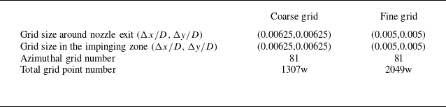
We have performed a grid independence check using two sets of grids, which is detailed in Appendix A. The mean flow field results obtained from these two grids are in good agreement. Additionally, the frequency and amplitude of the impinging tone, which is the main focus of this study, demonstrate minimal variation between the two grids. Therefore, the grid convergence is believed to be achieved, and the finer grid is selected for subsequent analysis. The total number of grid points is approximately 20.49 million. The grid is axisymmetric in the domain where the radial distance
 $r/D\gt 0.01$
, with 81 points uniformly distributed in the azimuthal direction, while a Cartesian grid block is put in the centre of the computational domain to avoid singularity. The specific grid distribution in the x–r plane is shown in figure 2(a). In the vicinity of the nozzle exit, as well as in the vicinity of the impinging region near the plate, the grid sizes are constantly
 $0.005D$
axially. In the jet core region, the grid axial sizes have a slight stretch, but the maximum grid size is only
 $0.0053D$
. The radial grid sizes are kept homogeneous as
 $0.005D$
in the range where radial distance
 $r/D \le 0.75D$
. The radial grid sizes are kept homogeneous as
 $0.005D$
in the range where radial distance
 $r/D \le 0.75D$
, and stretched with a constant stretch ratio of approximately
 $1\,\%$
where
 $r/D \gt 0.75D$
.
Figure 2(b) illustrates the computation domain as well as the boundary condition (BC) configuration. In this simulation, non-reflective radiation and outflow boundary conditions (Tam & Webb Reference Tam and Webb1993; Tam & Dong Reference Tam and Dong1996) are used at far-field boundaries. The no-slip boundary conditions incorporated with the ghost point method proposed by Tam & Dong (Reference Tam and Dong1994) are implemented on the nozzle lip, nozzle wall and the impinging plate. At the nozzle exit, all non-dimensional flow variables are given as follows:
 \begin{align} \rho _e=\frac {\gamma (\gamma +1) p_e }{ 2T_r }, \ \ p_e=\frac {1}{\gamma }\ \ \left [ \frac {2+(\gamma -1)Ma_j^2}{\gamma +1}\right ]^\frac {\gamma }{\gamma -1}, \ \ u_e=\left (\frac {2}{\gamma +1} \right )^\frac 12, v_e=0, w_e=0 \end{align}
where
 $T_r=T^* /T_\infty$
is the nozzle temperature ratio which is set to be 1 since the present case is a cold nozzle and the subscript
 $e$
represents the exit state.
(a) Grid distribution in the x–r plane displayed every 10 points. (b) Simulation domain and boundary condition configuration.

3. Simulation results
3.1. Mean flow fields
In this simulation, the CFL number is set to 0.4. The final data are beginning to be exported when the simulation runs after approximately 200 000 time steps and any start-up transients have left the computational domain. The mean flow field is obtained by averaging data from 300 000 time steps.
The density gradient amplitude field presented in figure 3(a) clearly shows the shock structures of the supersonic impinging jet. As illustrated in the figure, an expansion fan is observed to emanate from the nozzle lip, accompanied by the oblique shock generated by its reflection at the shear layer. Because the jet is highly under-expanded and the impinging plate is presented downstream, a normal shock (Mach disk) appears in the core. The Mach disk serves to terminate the oblique shock and is accompanied by a shock triple point and a slip line. The slip line, an axisymmetric embedded shear layer, separates the subsonic flow downstream of the Mach disk from the supersonic flow downstream of the reflected shock. This can be seen in the mean density field and streamline distribution in figure 3(b). In this context, the flow downstream of the Mach disk and the reflected shock are designated as central flow and peripheral flow, respectively. Since the reflected shock is bounded between the outer shear layer and the slip line, the reflection of shock-expansion waves will recur in the peripheral flow region.
Computed mean density in the x–y plane: (a) density gradient amplitude and (b) density and streamlines.

The stagnation pressure
 $p^*$
distribution in the x–y plane is presented in figure 4(a). The static pressure distribution is also shown where the jet structures are clearer. It can be observed that the central flow passes through the Mach disk, while the peripheral flow undergoes a series of oblique shocks. Because the stagnation pressure loss across the normal shock is considerably greater than that across the oblique shock, the stagnation pressure in the peripheral flow region is much higher than that in the central flow region, which is shown clearly in figure 4(b). Consequently, the static pressure of the peripheral flow is higher than that of the central flow near the wall, which drives the peripheral flow moving towards the centre and the formation of the recirculation bubble shown in figure 3(b).
(a) Mean stagnation pressure (upper half) and static pressure (lower half) distribution in the x–y plane. (b) Mean stagnation pressure distribution in the y–z plane in the wall surface.

The comparison of the computed mean axial velocity along the jet axis with the experimental results (Henderson et al. Reference Henderson, Bridges and Wernet2005) is presented in figure 5(a), in addition to the numerical results by other researchers (Dauptain, Cuenot & Gicquel Reference Dauptain, Cuenot and Gicquel2010; Gojon & Bogey Reference Gojon and Bogey2017). It is shown that the Mach disk is located at approximately
 $x/D=1.0$
, which agrees well with the experimental data and the two referenced numerical results. Upstream of the Mach disk, the present simulation results are consistent with the other two numerical simulations, but they are all larger than the experimental values. According to Dauptain et al. (Reference Dauptain, Cuenot and Gicquel2010), this discrepancy is attributed to the inertial effect of the digital particle imaging velocimetry (DPIV) measurement method employed in the experiments. This effect manifests in regions of strong acceleration, resulting in smaller measurement values. Downstream of the Mach disk, a distinct recirculation bubble with negative axial velocity is observed. The intensity and distribution range of this recirculation bubble in the present simulation agree well with the experimental measurement. Figure 5(b–d) present a comparison of the mean axial velocity distributions in the radial direction at
 $x/D = 0.75, 1.5$
and
 $1.8$
in the x–y plane, respectively. At
 $y/D = 0$
in figure 5(b,c), the numerical simulation results differ from the experiments due to the inertial effect of DPIV. Apart from this discrepancy, the results of this study are generally consistent with the reference data, affirming the accuracy of the present simulation.
Mean axial velocity distribution along different lines: (a) axis; (b)
 $x/D=0.75$
; (c)
 $x/D=1.5$
and (d)
 $x/D=1.8$
. The black solid lines represent the present simulation results. The red and green dashed lines represent the simulation data from Gojon & Bogey (Reference Gojon and Bogey2017) and Dauptain et al. (Reference Dauptain, Cuenot and Gicquel2010), respectively. The blue dashed lines represent the experimental data provided by Henderson et al. (Reference Henderson, Bridges and Wernet2005).

3.2. Instantaneous flow fields
The instantaneous density gradient amplitude field in the x–y plane, as shown in figure 6(a), distinctly reveals the presence of expansion waves, shock cells and the wall jet. Notably, the shear layer is marked by considerable instability, leading to the formation of KH vortices. These vortices are amplified as they convect downstream, and then impinge on the wall and alter their trajectory towards the radial direction. The slip stream, which is also a shear layer, generates KH vortices, too. These vortices convect downstream and merge into the wall jet.
The instantaneous pressure field in the x–y plane, depicted in figure 6(b), reveals strong acoustic waves emanating from the impingement region. These waves appear to be concentric and nearly equally spaced, suggesting that the current supersonic impinging jet produces significant tonal noise. The instantaneous pressure distribution in the y–z plane at
 $x/D=-1.5$
is shown in figure 6(c), where the impinging tone displays distinct axisymmetric feature.
Instantaneous flow fields of (a) density gradient amplitude in the x–y plane, (b) pressure in the x–y plane and (c) pressure in the y–z plane.

A sketch of sampling points location (in
 $x=0$
plane).

3.3. Acoustic results
As illustrated in figure 7, 40 points uniformly spaced in the azimuthal direction at
 $r/D=1$
in the nozzle exit plane are used for time tracing the pressure signal. The computed power spectral density (PSD) and sound pressure level (SPL) of the sampled pressure signals are presented in figure 8. The PSD data are averaged over all the monitor points, generating a azimuthal averaging result. The SPL data are from the monitor point that has the maximum main tone amplitude. It is clear that there are multiple distinctive tone components, with the dominant component having a Strouhal number of
 $St=fD_j/u_j=0.5262$
, where
 $D_j$
and
 $u_j$
represent the fully expanded diameter and velocity, respectively. The frequencies of the other tone components are
 $St=0.386,1.062$
. The component with
 $St=1.062$
corresponds to the second harmonic of the dominant tone, while that with
 $St=0.386$
represents another distinct tone, termed as the secondary tone.
Computed noise spectra: (a) power spectral density; (b) sound pressure level.

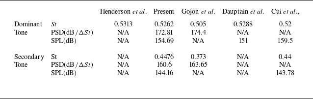
Figure 8 presents a comparison of the present noise spectra with the data from three other researchers (Dauptain et al. Reference Dauptain, Cuenot and Gicquel2010; Gojon, Bogey & Marsden Reference Gojon, Bogey and Marsden2015; Gojon & Bogey Reference Gojon and Bogey2017; Cui et al. Reference Cui, Xu, Wang, Zhang and Qin2021). A summary of the tone noise component comparison is provided in table 1. The dominant tone frequency results of the reference are
 $St=0.505,0.5288$
and
 $0.52$
. Furthermore, the experimental value is
 $0.531$
(Henderson et al. Reference Henderson, Bridges and Wernet2005; Dauptain et al. Reference Dauptain, Cuenot and Gicquel2010). The present simulation result closely aligns with those of Dauptain et al. (Reference Dauptain, Cuenot and Gicquel2010) and Cui et al. (Reference Cui, Xu, Wang, Zhang and Qin2021), both of which exhibit a high degree of concordance with the experimental data. However, the dominant tone frequency reported by Gojon et al. (Reference Gojon, Bogey and Marsden2015); Gojon & Bogey (Reference Gojon and Bogey2017) is slightly lower. The present simulation yields a PSD of the dominant tone at
 $172.81 \, {\rm dB}/\Delta St$
, and the value reported by Gojon et al. (Reference Gojon, Bogey and Marsden2015); Gojon & Bogey (Reference Gojon and Bogey2017) is
 $174.4 \, {\rm dB}/\Delta St$
. The present simulation yields an SPL result of
 $154.7 \, {\rm dB}$
. The value reported by Dauptain et al. (Reference Dauptain, Cuenot and Gicquel2010) is
 $151 \, {\rm dB}$
, while Cui et al. (Reference Cui, Xu, Wang, Zhang and Qin2021) documented a higher result of
 $159.5\, {\rm dB}$
. Although there is a discrepancy in the amplitude, the value of the present simulation falls in between.
In addition to the tone components, the amplitudes of broadband shock-associated noise in this simulation are in agreement with those reported by Gojon et al. (Reference Gojon, Bogey and Marsden2015); Gojon & Bogey (Reference Cui, Xu, Wang, Zhang and Qin2017) and Cui et al. (Reference Gojon and Bogey2021). However, the broadband noise level reported by Dauptain et al. (Reference Dauptain, Cuenot and Gicquel2010) is considerably lower. This discrepancy can be primarily attributed to the Taylor–Galerkin method employed for spatial discretisation in their study, which introduced much more dissipation and constrained the capture of small-scale structures, resulting in a reduced intensity of broadband noise. Overall, the spectrum results of the present simulation show good agreement with the reference data.
Comparison of the tone frequencies and amplitudes.

To determine the azimuthal modes of the tones in the present simulation, an azimuthal correlation analysis is conducted on the pressure signals sampled at the 40 points shown in figure 7. The variations of the relative phase
 $\varphi$
for the dominant and secondary tones are presented in figure 9(a). The amplitude variation of tones along the azimuthal direction is also plotted in figure 9(b). It is shown that the variation of the relative phase for the dominant tone is less than
 $15^\circ$
, and the variation of the SPL in the azimuthal direction is less than
 $3.5\,{\rm dB}$
. Therefore, it can be concluded that the mode of the dominant tone is axisymmetric.
Azimuthal characteristics of the dominant and secondary tones: (a) relative phase distribution; (b) amplitude directivity pattern.

Gojon & Bogey (Reference Gojon and Bogey2017) analysed the modes of the impinging tones by Fourier decomposition of the pressure field. According to their results, the mode of the secondary tone was helical. The variations of the azimuthal phase and the SPL are plotted in figure 9 for the secondary tone in this simulation. It is shown that the relative phase angle
 $\varphi$
varies in a sinusoidal mode in the azimuthal direction, and the amplitude directivity pattern consists of two lobes with a significant difference in intensity. It implies that the secondary tone obtained in the present simulation is flapping mode.
DMD analysis results: (a) the norms of the DMD modes; (b) the amplitude distribution of the dominant mode in
 $z=0$
plane; (c) the amplitude distribution of the dominant mode in
 $x=0.53$
plane.

3.4. Dynamic mode decomposition analysis
The dynamic mode decomposition (DMD) (Schmid Reference Schmid2010) is employed in this study to further investigate the dominant modes of the flow field. One-hundred-and-twenty-five snapshots of the density field are used for analysis, in which the time interval between two adjacent snapshots is
 $0.0828D_j /U_j$
. Figure 10(a) demonstrates the distribution of the resultant DMD mode norms. It is evident that, apart from the mean mode with
 $St=0$
, the supersonic impinging jet flow field is dominated by the mode with frequency
 $St=0.529$
. This frequency is coincident with the dominant tone frequency, revealing a relationship between the flow field and the tone noise.
The contour of the dominant mode in the
 $z=0$
plane is plotted in figure 10(b), in which there are clearly tone waves. Figure 10(c) demonstrates the contour of the dominant mode in the
 $x/D=1.53$
plane. It can also be observed that both the dominant modes of the flow and acoustic fields are axisymmetric.
The DMD results show that the dominant oscillatory mode of the flow field not only possesses the same frequency as that of the dominant tone, but also the axisymmetric mode. This indicates an inherent connection between the dominant modes of the flow field and the impinging tone. In the next section, a phase-locked averaging analysis is conducted to provide insights into the underlying mechanisms and the relationship between the flow field oscillation and impinging tone generation.
4. Phase-locked averaging analysis
To observe the oscillation process of the jet structure more clearly, a phase-locked averaging analysis is performed to eliminate irrelevant disturbances. The impinging jet flow fields are sampled with time interval
 $\Delta t = 0.02376D_j/u_j$
. Reminding that the dominant tone frequency in the present simulation is
 $St=0.5262$
, there are 80 snapshots in a single period of the dominant tone with this sampling frequency. Totally, 2960 snapshots are sampled for phase-locked averaging, corresponding to 27 tone periods. Therefore, it is reasonable to believe that the resulted phase-locked averaged fields basically retain only the oscillatory processes associated with the dominant tone.
As mentioned previously, both the dominant tone and DMD mode are in axisymmetric mode. Therefore, only the results in the x–y plane are demonstrated in the following subsections.
4.1. The motion of the Mach disk and the reflected shock
The evolution of the near-field streamlines and pressure within one period is depicted in figure 11. In each panel of figure 11, the two black vertical bars near the Mach disk indicate the extreme positions of the Mach disk movement. To illustrate the motion of shocks more clearly, the pressure distribution along the axis and the line at
 $y/D=0.35$
during one dominant tone period are shown in figures 12(a) and 12(b).
Supersonic impinging jet structure and streamline oscillation, and the progression of pressure variation.
 $V1$
,
 $V2$
and
 $V3$
represent three KH vortices.
 $R1$
and
 $R2$
indicate the recirculation bubbles.
 $H$
labels the high-pressure fluid mass. The white arrows indicate the local streamline directions. The vertical black bars in the axis are extreme positions of the Mach disk movement.

Pressure distribution variation at different times within one dominant tone period, across (a) the Mach disk and (b) the reflected shock. The location and pressure variation at (c) the tail of the Mach disk, (d) the head of the reflected shock and (e) the tail of the reflected shock within one dominant tone period, where the black and red dots represent the shock location and pressure variation, respectively, and the black and red curves represent the fitted sinusoidal curves.

As shown in figure 12(a), the axial pressure distribution varies periodically, indicating that the Mach disk is oscillating in a periodic horizontal motion. The flow field upstream of the Mach disk is almost steady, while the pressure downstream of the Mach disk oscillates periodically. To show the trajectory of the Mach disk movement, the tail of the Mach disk is labelled with magenta circles in figure 12(a). These circles are defined as the points where the pressure derivative along the axis is closest to 6. The corresponding location
 $\xi$
and the pressure of the tail are plotted in figure 12(c). It can be seen that the Mach disk moves upstream in the first half-period and downstream in the second half-period. The pressure at the tail also exhibits a similar sinuous trend, but with a
 $T/4$
phase lag, where
 $T$
is the period of the dominant tone.
The pressure variation of the reflected shock is presented in figure 12(b). Similar to the Mach disk, the reflected shock is also oscillating in a periodic motion. Differently, the flow fields upstream and downstream of the shock are both notably disturbed. The magenta circles in figure 12(b) indicate the head and the tail positions of the shock, and the corresponding location
 $\xi$
and pressure variation are plotted in figures 12(d) and 12(e), respectively. It is clear that the location and the pressure are oscillating in the same sinuous mode as that of the Mach disk. Comparing the location variations of the head and tail of the reflected shock, there is a phase difference of
 $0.0018 \pi$
. There is also a phase difference between the pressure variations, which is approximately
 $0.00215 \pi$
. These phase differences are a result of the time taken by pressure disturbance propagating through the shock, which is so small that the head and the tail of the reflected shock are believed to be moved synchronically.
Comparing the location variations of the Mach disk and the reflected shock, it can be seen that there is also a phase difference of approximately
 $0.0003 \pi$
, which is also so small that the oscillation motion of these shocks can be considered to be synchronised. Comparing the pressure variations between the Mach disk and the reflected shock, the phase downstream of the reflected shock is
 $T/4$
ahead of the Mach disk. If we assume the pressure disturbance was propagating from the downstream of the reflected shock to that of the Mach disk, the propagation speed can be estimated to be approximately
 $0.85 c_\infty$
with the phase lag and distance between the two sampling positions, which are at
 $y/D=0.35$
and
 $y/D=0$
, respectively. The time averaged mean sound speed
 $c_a$
of the flow is plotted in figure 13. It is found that the acoustic speed downstream of the reflected shock is very close to that of the Mach disk, which is approximately
 $0.9 c_\infty$
. Furthermore, if we integrate the actual propagation speed,
 $c_a -v$
from
 $y/D=0.35$
to the axis to take the convection effect into consideration, the resultant value is
 $0.8405 c_\infty$
. This value is very close to the estimated speed above with the phase lag and distance between the two sampling points. This suggests that the phase difference in pressure variation arises due to the time required for the propagation of pressure disturbances.
Note that when the pressure around the reflected shock changes, it will not move significantly due to the constraints imposed by the Mach disk in the presence of shock triple reflection. The reflected shock will only move if the pressure disturbance propagates downstream of the Mach disk, causing it to move.
Contour of the mean acoustic speed
 $c_a$
in the x–y plane.

As to the cause of the pressure variation, the answer can be found by observing the motion of the jet plume in the vicinity of the shocks, as shown in figure 11. In the time interval
 $t/T=0{-}4/8$
, the corresponding snapshots of which are figure 11(a–e), the vortex
 $V2$
convects from upstream of the shock to downstream. It is known that the pressure in the region between vortices
 $V1$
and
 $V2$
is higher than that at the vortex centre. Therefore, as the vortex passes through the shock, the pressure downstream of the shock should decrease, which is consistent with the pressure variation trend shown in figure 12(d–e). In the time interval from
 $4/8T$
to
 $T$
, the corresponding snapshots of which are shown in figure 11(e–i), the vortex
 $V2$
convects away from the reflected shock and another vortex
 $V3$
approaches the reflected shock tip. This causes the pressure downstream of the shock to increase, as shown in figure 12(d,e). The pressure around the reflected shock varies in coordination with the convective motion of the KH vortices, so it is the convective motion of KH vortices that causes the pressure perturbation around the reflected shock. As analysed previously, this pressure perturbation will propagate to the downstream of the Mach disk, causing the Mach disk as well as the reflected shock to oscillate.
4.2. The oscillation process in the recirculation region
The oscillation process in the recirculation region is analysed in detail in this subsection, and the entire oscillation period is divided into four stages based on the Mach disk oscillation. The first stage is shown in figure 11(a–c). During this stage, the Mach disk moves upstream from the rightmost position. The shock motion is more evident in figure 12(c). At the same time, a mass of high-pressure fluid
 $H$
is observed to shed from the Mach disk and compress the recirculation bubble
 $R1$
.
In the second stage shown in figure 11(c–e), the Mach disk continues its upstream movement, eventually reaching the leftmost position. Meanwhile, the recirculation bubble
 $R1$
is compressed as the high-pressure fluid mass
 $H$
continues to approach the impinging plate. After figure 11(d), the recirculation bubble
 $R1$
is compressed into the corner region of the central flow and the recirculation structure eventually disappears from the centre. Subsequently, as shown in figure 11(e), a new recirculation bubble
 $R2$
is rapidly generated in the flow field.
In the process shown in figure 11(d,e), it can be seen that the central flow recirculation nearly vanishes with the evolution of the recirculation bubble
 $R2$
. The pressure in the vicinity of the impinging plate reaches a very high level and the velocity approaches zero. Consequently, the flow field in this region is in an unstable state, which inevitably leads to the formation of a recirculation. Figure 14 shows the
 $Q$
-criterion distribution and the streamlines at the instance when
 $R2$
is generated. The
 $Q$
-criterion is defined as the difference between the anti-symmetric tensor
 $B$
and the symmetric tensor
 $A$
of the strain tensor
 \begin{equation} Q=(|B|_F^2-|A|_F^2)/2, \end{equation}
where
 $|\ |_F$
is the Frobenius norm of the matrix. In the context of the
 $Q$
-criterion, a positive value of the
 $Q$
indicates the dominance of fluid rotation, signalling the presence of vortices. Conversely, a negative value of
 $Q$
suggests shear dominance. According to the
 $Q$
-value contour shown in figure 14, there are periodically distributed positive Q values at the shear layer of the jet and the slip line downstream of the Mach disk. These positive values denote the presence of KH vortex structures in these regions. The recirculation bubble
 $R2$
is formed at the position
 $P$
labelled in figure 14, where a slip line KH vortex just reaches. Furthermore, based on the velocity difference between the central and peripheral flow, it can be determined that the vortex rotates counterclockwise, which is consistent with the direction of the recirculation bubble. Due to the unstable state of the local flow, the KH vortex acts as a trigger, and a new recirculation bubble
 $R2$
appears at point
 $P$
.
 $Q$
-criterion and streamlines distribution in the second stage of oscillation (
 $Q$
values in the contour are uniformly distributed from –10 to 10 in 21 layers).

In the third stage shown in figure 11(e–g), the Mach disk moves downstream. Downstream of the Mach disk, a high-pressure fluid mass
 $H$
begins to detach, convecting downstream and compressing the newly formed recirculation bubble
 $R2$
which gradually merges with
 $R1$
.
In the final stage of the oscillation demonstrated in figure 11(g–i), the Mach disk continues to move downstream and eventually reaches the rightmost position. Meanwhile, the high-pressure fluid mass
 $H$
continues to move downstream, compressing the recirculation bubble
 $R1$
, and persists until the start of the next cycle.
4.3. Recirculation bubble oscillation mechanism
According to Ginzburg et al. (Reference Ginzburg, Semiletenko, Terpigor’ev and Uskov1970), the motion of the recirculation bubble is closely related to the oscillation of the Mach disk. They believed that the pressure in the recirculation region is lower than that in the peripheral flow, resulting in the fluid accumulation in the central region. The pressure then rises, making the bubble size increase and the Mach disk to move upstream. The fluid in the central region leaks into the peripheral region, causing the pressure to drop and the Mach disk to move downstream. This reduces the size of the recirculation bubble. According to this view, the recirculation bubble is characterised by a periodic reciprocating motion, and the direction of the recirculation bubble boundary motion is the same as that of the Mach disk.
However, according to the analysis of the motion of the recirculation bubble presented in figure 11, the oscillation process is characterised by a periodic ‘compression–generation–merging’ cycle, which is different from the view of Ginzburg et al. (Reference Ginzburg, Semiletenko, Terpigor’ev and Uskov1970). The Mach disk moves upstream during the first half of the period (i.e. Figure 11 a–e), and the recirculation bubble gradually becomes smaller until it is compressed into the corner of the central flow. In the second half of the period (i.e. Figure 11(e–i), the Mach disk moves downstream, and the recirculation bubble undergoes generation, merging and compression. It is evident that the recirculation bubble is compressed until its disappearance in the central region, after which a new bubble is generated and continues to be compressed. This periodic motion was not anticipated by the perspective of Ginzburg et al.
According to the previous analysis, the pressure disturbance downstream of the Mach disk, which is propagated from the KH vortex, induces the Mach disk to oscillate. As the Mach disk begins to move downstream, i.e. Figure 11(f–h), the high-pressure fluid mass
 $H$
starts to shed, and this mass directly drives the motion of the recirculation bubble. Thus, in our view, the motion of the recirculation bubble is the resultant manifestation of the motion of the Mach disk, rather than the interaction between these two structures as the view of Ginzburg et al., holds. Therefore, the KH vortices are the fundamental driving force for the periodic motion of the recirculation bubble.
4.4. Streamline oscillation analysis
The oscillation process of the pressure and streamlines near the wall jet is presented in figure 15. It is observed that the KH vortices are emanated from the nozzle lip and amplified in the shear layer as they convect downstream. When the KH vortices reach the impingement region, they become large enough to be recognised from streamlines. The KH vortices then turn towards the wall jet, gradually weaken and eventually merge with the wall jet. As the KH vortex convects and passes through the wall jet boundary, it disturbs the shear layer of the wall jet, causing the streamline to oscillate.
In figure 15, the white arrows labelled in the wall jet indicate the direction of the streamline in the outer area of the wall jet. From figure 15(a–c), the streamlines gradually flap to the right and align with the wall jet. At the same time, the upper edge of the KH vortex
 $V1$
passes through the position marked by the white arrow. Then, from figure 15(c–g), the streamlines continue to flap to the right, pointing towards the wall. Meanwhile, the lower edge of
 $V1$
passes through this point gradually. From figure 15(g–i) and the beginning of the next cycle, the streamlines flap to the left, accompanied by the departure of
 $V1$
and the approach of
 $V2$
. Similar observations were made by Henderson et al. (Reference Henderson, Bridges and Wernet2005), who reported periodic variation of the direction of the velocity vector and wall jet oscillations at the radial position
 $1.3D$
. They attributed impinging flow oscillations to the periodic motion of the wall jet and the consequent generation of the impinging tone. Based on the flow field motion illustrated in figure 15, it can be seen that the oscillation of the streamline and the passage of KH vortices are synchronised; therefore, it is believed that the oscillation of the streamline is the entrained flow caused by the passage of the KH vortex.
Additionally, the process of tone wave emission, as presented in figure 15(a,b), is synchronised with the impingement of KH vortices. This means when the KH vortex impinges on the wall jet, the tone wave is emitted from the impingement point at the same time. Thus, it can be hypothesised that the tone generation mechanism may also be related to the impinging collision of KH vortices. In the next subsection, more evidence will be provided to support this view.
Progression of the wall jet streamline oscillation and pressure variation. The labels are the same as those in figure 11.

4.5. Sound ray analysis
In this section, the sound ray method is applied to investigate the phase field of the dominant tone. Using the phase-locked averaged data, the phase field can be calculated by Fourier transform, as shown in figure 16(a). Assuming that the region far away from the jet plume has little variation in sound velocity, the phase contour lines are assumed to be the wavefronts and the corresponding sound source information can be derived from the direction of the inner normal lines using the Huygens principle. These lines are referred to as sound rays. First, seven wavefronts with phases ranging from
 $0.2$
to
 $6$
are extracted. Then they are shifted along the sound rays to the line with the phase
 $\pi$
, as shown in figure 16(b). These lines are almost coincident with each other with only a small deviation. The small deviation is due to the fact that some wavefronts have touched the nozzle wall, resulting in the shape being influenced by the reflected sound waves and gradually becoming perpendicular to the nozzle wall. The sound source information in these wavefronts is contaminated. In this study, the wavefront with a phase of 0.5 is chosen for the sound ray analysis, which is marked as a white line in figure 16(a).
(a) Phase field of the phase-locked averaged fields and the feedback loop path. (b) Comparison of phase contour lines which are shifted to the same phase
 $\pi$
along the sound rays.

As shown in figure 17, by retracing the sound rays, it is indicated that the wavefront can be divided into two parts, implying the tone is emitted from two distinct sources. The upper part of the wavefront converges at the location where the KH vortices impinge on the plate. Recalling the analysis of the streamline oscillation in figure 11, it is evident that the emission of tone waves is synchronised with the KH vortex impinging on the wall. Therefore, it can be deduced that this part of the wavefront originates from the KH vortices impinging on the wall, i.e. the vortex collision mechanism (Tam & Ahuja Reference Tam and Ahuja1990; Edgington-Mitchell Reference Edgington-Mitchell2019). The lower part of the wavefront is directed towards the wall jet area, with its source roughly located at the radial position
 $1.1D{-}1.4D$
. This position coincides with the location of the wall jet oscillation, as observed in figure 15 and corroborated by the data from Henderson et al. (Reference Henderson, Bridges and Wernet2005) and Jia, Gao & Hu (Reference Jia, Gao and Hu2023). This consistency confirms the presence of the wall jet oscillation mechanism proposed by Henderson et al. (Reference Henderson, Bridges and Wernet2005) in the current simulation. Therefore, based on the analysis of the present numerical results, it can be concluded that these two tone generation mechanisms coexist and contribute to the impinging tone acoustic field.
Gojon & Bogey (Reference Gojon and Bogey2017) also found that there are two sound sources in the impinging region in their numerical simulations, and they suggested that the source near the axial position plays a role in the feedback loop. However, according to the theory of the feedback loop mechanism (shown in figure 1), the feedback waves should propagate back to the nozzle lip, inducing a new initial disturbance in the shear layer. As illustrated in figure 17, the two sound sources have different directivity. The sound waves from vortex collision propagate mainly at an angle less than
 $50^\circ$
inclined with the wall, while the sound waves from the wall jet oscillation propagate primarily towards the nozzle lip. Therefore, it is the wall jet oscillation mechanism that drives the tone generation process in the feedback loop.
Results of sound ray analysis and pressure field. The white and the magenta arrows indicate the propagation direction of the waves generated by the wall jet oscillation and vortex collision, respectively.

Phase variation along the feedback loop path. The line colours are consistent with that of the path in figure 16(a).

The feedback loop path can be inferred from the phase distribution, as shown by the solid lines in figure 16(a). The phase variation along the feedback loop is shown in figure 18. The KH vortices propagate downstream along the magenta line, resulting in a gradual decrease in phase along the
 $x$
-direction. It is observed that the amplitude of the instability waves is significantly smaller than that of the tone waves near the nozzle lip. Consequently, the phase variation is predominantly influenced by the tone waves, leading to an increase along the
 $x$
-direction within the range of
 $x\lt 0.4$
, as shown in figure 18. The tone waves propagate back to the nozzle lip along the cyan solid line, with their phase gradually increasing along the
 $x$
-direction.
In most of the proposed views on the impinging tone (Dauptain et al. Reference Dauptain, Gicquel and Moreau2012; Edgington-Mitchell Reference Edgington-Mitchell2019), the tone is generated at the wall and the length of the feedback loop path is equal to the impinging distance. However, as shown in figure 16(a), the tone waves are actually emitted from the intersection of the cyan and black lines, the distance from which to the wall is approximately
 $1.636D$
. Along the black solid line, the phase varies little as shown in figure 18, indicating that the tone generation occurs in a distributed region. Additionally, the phase contour lines in the wall jet region are approximately perpendicular to the wall. This suggests that the wall jet oscillates as a whole to generate tone waves.
From the data on phase variation, it can be obtained that the distance over which the KH vortices convect in the feedback loop is approximately
 $1.4D$
, and the distance for the tone waves to propagate back to the nozzle lip is roughly
 $1.636D$
. This suggests that the average convection speed of the KH vortices is approximately
 $0.428c_\infty$
, which is smaller than the value range of
 $0.6\sim 0.8 c_\infty$
proposed by André (Reference André2012). This discrepancy may be attributed to the influence of the plate that is placed too close. Considering (1.1), if we take into consideration the difference between the upstream and the downstream propagating distances as well as the averaged value of the downstream propagation speed, the tone frequency prediction formula can be rewritten as follows:
 \begin{equation} f = \frac {N+p}{ h_1/\bar {u}_c + h_2/u_a }. \end{equation}
According to the phase variation in figure 18, there are two periods for the downstream propagating waves and one period for the upstream propagating tone in the feedback loop. Therefore,
 $N=3$
and
 $p=0$
are obtained. The downstream convection distance is
 $h_1=1.4D$
and the upstream propagation distance of tone waves is
 $h_2=1.636D$
. Taking the averaged convection speed of the downstream propagating instabilities as
 $\bar {u}_c=0.428c_\infty$
and the propagation speed of the tone as
 $u_a=c_\infty$
, the predicted frequency is
 $St=0.5273$
according to (4.2). This is consistent with the value
 $0.5262$
computed in the simulation directly. This implies that the above analysis about the feedback loop and tone generation mechanism is reasonable.
It is worth emphasising that, according to the previous analysis, the feedback loop is established outside the jet. While the motion of jet structures, such as the Mach disk and the recirculation bubble, is fundamentally driven by the pressure change due to the passage of KH vortices, it can be argued that the oscillations of jet structure are merely a byproduct of the feedback loop. They oscillate simply because they are interconnected with and thus influenced by the feedback loop. Additionally, Henderson et al. (Reference Henderson, Bridges and Wernet2005) analysed a series of experimental data and found that impinging jets can emit tone noise regardless of the presence or absence of recirculation bubbles, indicating that the recirculation bubble is not a key element in tone generation. This is consistent with the analysis in this study.
5. The feedback loop and jet oscillation mechanism of the supersonic perpendicular impinging tone
Summarising the previous analysis, we propose an improved view of the tone generation and the oscillation of the supersonic perpendicular impinging jet, as well as their relationship. Two mechanism sketches are illustrated in figure 19.
Sketches explaining the tone generation and the jet structures oscillation of supersonic perpendicular impinging jets. (a) The shock structures move to the right. (b) The shock structures move to the left.

First, the feedback loop mechanism occurring outside the jet is the fundamental mechanism for the impinging tone. The large-scale instability wave originating from the KH instability, the wall jet oscillation, the upstream propagating tone waves and the nozzle lip receptivity constitute the four key elements of the loop.
Second, the sound field of tone is contributed by two sources, the wall jet oscillation source in the feedback loop and the vortex collision source. In the loop, the KH vortices induced by the KH instability grow stronger by drawing energy from the main flow. When they impinge on the wall, they break up and can also generate acoustic waves. These acoustic waves, together with those from the wall jet oscillation in the feedback loop, make up the entire sound field. The waves from these two sources have different directivity. As shown in figure 19, waves from the vortex collision propagate mainly in the downstream direction of the wall jet, while the others propagate towards the nozzle lip. This difference in directivity explains why the wall jet oscillation mechanism participates in the feedback loop while the other does not.
Third, the impinging jet plume is motivated by KH vortices and thus suffers forced oscillation. The presence of KH vortices in the jet shear layer also implies the presence of periodic pressure perturbations: the pressure is relatively low in the centre of KH vortices, while the pressure is relatively high in the region between the two adjacent vortices. These pressure perturbations are illustrated in figure 19 with the red and blue band at the jet shear layer. The region where vortices appear possesses relatively lower pressure and is indicated in blue, and vice versa in red. At the tip of the reflected shock, the periodic passage of KH vortices results in pressure perturbations around the shock, leading to oscillations of both the reflected shock and the Mach disk. The Mach disk interacts with the pressure perturbations and generates a mass of high-pressure flow as the Mach disk moves to the right shown in figure 19(a). This mass of high-pressure flow moves downstream and drives the motion of the recirculation bubble to undergo a periodic ‘compression–generation–merging’ process. When convecting downstream, the high-pressure flow mass compresses the bubble to the central flow region corner. Upon reaching the plate, as shown in figure 19(b), it makes the pressure near the plate higher than that behind the Mach disk. Along with KH vortices as a triggering factor, the fluid generates another recirculation bubble suddenly which merges with the previous one quickly.
Finally, the relationship among key elements in the feedback loop and jet plume oscillation is summarised and illustrated in figure 20. It is worth noting that the oscillatory behaviours of the reflected shock, the Mach disk and the recirculation bubbles are fundamentally driven by KH vortices. This implies that the oscillatory process within the jet structure is due to an additive effect of the feedback loop. Due to the spatial contact, these jet structure oscillations occur as forced oscillations.
Relationship among key elements in the feedback loop and jet plume oscillation.

6. Conclusions
To enhance the understanding of the impinging tone generation mechanism and the flow structure oscillation, a supersonic perpendicular impinging jet with a pressure ratio of 4.03 and an impingement distance of
 $2.08D$
is simulated. The computed mean flow field and noise spectra are compared with the experimental and numerical results of other researchers, and good agreement is obtained.
The oscillation process of the jet plume is discussed in detail. First, it is found that the recirculation bubbles show a periodical ‘compression–generation–merging’ motion process, and a mass of high-pressure fluid is found which plays a significant role in the bubble’s oscillation. In addition, the KH vortex convection serves as the driving force for not only the oscillation of the shock structures but also the oscillation of the recirculation bubble. As for the tone generation, it is found that two impinging tone noise sources, vortex collision and wall jet oscillation mechanisms, coexist in the impinging jet. Considering the different propagation directivity, the wall jet oscillation mechanism is believed to be the generation process in the feedback loop.
To summarise, an improved view is proposed. The KH instability in the jet shear layer and the wall jet oscillation mechanism constitute the downstream process and the generation process of the feedback loop, and this feedback loop mainly occurs outside the jet core. In addition, the impinging KH vortices also radiate acoustic waves, which compose the acoustic field in conjunction with those from the wall jet oscillations, but they do not contribute to forming the feedback loop. Finally, the periodic convection of KH vortices drives shocks to oscillate, which pulsates the fluid behind the Mach disk, especially the recirculation bubbles, causing them to oscillate periodically as well.
Funding.
This work is supported by National Natural Science Foundation of China (Grant number NSFC-51876003); National Science and Technology Major Project (Grant number J2019-II-0006-0026); and Science Center for Gas Turbine Project of China (Grant number P2022-A-II-003-001).
Declaration of interests.
The authors report no conflict of interest.
Appendix A. Grid independence test
To ensure grid independence, another coarser grid is tested in addition to that used in the main text. The grid employed in the main text is referred to as the fine grid, while the coarser grid is called the coarse grid. Both grids share the same topology, and the grid parameter comparison is summarised in table 2.
Grid parameters of the coarse mesh and fine mesh.

Comparison of mean axial velocity distribution for fine mesh and coarse mesh along different lines: (a) axis; (b)
 $x/D=0.75$
; (c)
 $x/D=1.5$
; (d)
 $x/D=1.8$
. The black solid lines and red dotted lines represent the results of the fine grid and coarse grid, respectively.

The comparison of the mean axial velocity along the jet axis is presented in figure 21(a). Although there are slight discrepancies behind the Mach disk, the axial velocity distributions for both the coarse and fine grids are consistent. The mean axial velocity distributions in the radial direction at
 $x/D = 0.75, 1.5$
and
 $1.8$
in the x–y plane are also compared, as shown in figure 21(b–d), which also demonstrate good agreement.
The power spectral density (PSD) spectra sampled from both grid sets are presented in figure 22. The main tone is captured in both grids, with a frequency difference of
 $\Delta St=0.0088$
and an amplitude difference of
 $\Delta {\rm PSD}=0.573\,{\rm dB}/\Delta St$
, indicating a very small deviation. Additionally, the overall broadband noise levels are consistent, with a small difference of approximately
 $1.5\,{\rm dB}/\Delta St$
.
In summary, the results from the coarse grid and the fine grid are consistent, confirming the mesh used in the context is sufficient for impinging jet and tone simulation.
Spectrum comparison for fine mesh and coarse mesh. The red and black lines represent the results from the coarse grid and fine grid, respectively.