1. Introduction
Planar jets are commonly found in a broad range of industrial applications and in several natural environments; examples include propulsion, injection of fluids, enhancement of mixing and many geophysical flows. The combination of a fundamental and practical interest drove many early experimental studies to characterise this flow configuration, mainly focusing on the well-known self-similar region, which arises at around 40 inlet-slot widths downstream of the injection point for large Reynolds numbers (Bradbury Reference Bradbury1965; Heskestad Reference Heskestad1965; Gutmark & Wygnanski Reference Gutmark and Wygnanski1976). Within the self-similar region, all flow quantities are independent of the streamwise distance from the inlet, once they are suitably rescaled using the similarity variables, i.e. the averaged streamwise velocity at the centreline and the jet thickness (Townsend Reference Townsend1980). In the self-similar region, the similarity variables show a constant-exponent power law scaling as a function of the distance from the inlet. However, planar jets present other intriguing properties, e.g. flow instabilities close to the injection point, vortex pairing, large- and small-scale entrainment at the jet interface, whose relevance changes with the Reynolds number. In this work, we address via direct numerical simulations (DNS) the Reynolds number dependence of the spatial development of an incompressible planar jet.
The relative simplicity of the planar-jet flow configuration has led to the development of asymptotic theories that hold in the limit of very large Reynolds numbers, and predict power-law behaviours in the self-similar turbulent region (Bradbury Reference Bradbury1965; Heskestad Reference Heskestad1965). More recently, a modified mean-field theory has been proposed by Cafiero & Vassilicos (Reference Cafiero and Vassilicos2019), which still predicts power-law behaviours but with reduced exponents. A theory has been derived also for laminar jets in the limit of vanishing Reynolds number (Mei Reference Mei2001), with power-law predictions for the centreline velocity and the jet width. Based on these theories, we have thus a fair understanding of the planar jet in the low-Reynolds-number laminar regime and in the high-Reynolds-number turbulent regime, where indeed the self-similar region provides a reasonable description of the entire flow field. However, theoretical predictions for intermediate Reynolds numbers, when the jet is in a transitional state being neither completely laminar nor completely turbulent, are missing. Several recent works (mainly based on experiments) have investigated planar jets at intermediate Reynolds numbers, in the range
 $10^2 \lesssim Re \lesssim 10^4$
, reporting the absence of a self-similar behaviour and a strong dependence of the flow properties on the actual Reynolds number (Namer & Ötügen Reference Namer and Ötügen1988; Deo, Mi & Nathan Reference Deo, Mi and Nathan2008; Suresh et al. Reference Suresh, Srinivasan, Sundararajan and Das2008).
A variation of the Reynolds number largely influences the near-inlet flow, i.e. the onset of the flow instabilities and the transition to turbulence. Close to the inlet, the centreline velocity is almost constant in the so-called potential core, which spans around 10 inlet-slot widths from the inlet. When the Reynolds number increases, the length of the potential core tends to decrease due to an anticipated flow transition (Namer & Ötügen Reference Namer and Ötügen1988; Deo et al. Reference Deo, Mi and Nathan2008; Suresh et al. Reference Suresh, Srinivasan, Sundararajan and Das2008). The Reynolds number also determines the leading mode that promotes transition to turbulence in the near-inlet region. The generation of the Kelvin–Helmholtz (KH) vortices in the shear layers is indeed antisymmetric (sinusoidal mode) with respect to the centreline for low Reynolds numbers, while symmetric (varicose mode) for large Reynolds numbers (Sato Reference Sato1960; Beavers & Wilson Reference Beavers and Wilson1970; Wygnanski & Gutmark Reference Wygnanski and Gutmark1971; List Reference List1982; Antonia et al. Reference Antonia, Browne, Rajagopalan and Chambers1983; Thomas & Goldschmidt Reference Thomas and Goldschmidt1986; Thomas & Chu Reference Thomas and Chu1989; Thomas & Prakash Reference Thomas and Prakash1991; Da Silva & Métais Reference Da Silva and Métais2002; Stanley, Sarkar & Mellado Reference Stanley, Sarkar and Mellado2002; Deo et al. Reference Deo, Mi and Nathan2008). The different symmetry of the unstable modes also leads to a different frequency of vortex formation, which is generally lower for the varicose mode. The non-dimensional frequency (Strouhal number)
 $St = f h/V_0$
of the two modes has been found to be roughly independent of the Reynolds number, when large enough (
 $Re \gtrapprox 2000$
): for the sinusodal mode, Deo et al. (Reference Deo, Mi and Nathan2008) found a value of
 $St\approx 0.1$
, while Ko & Davies (Reference Ko and Davies1971), Namer & Ötügen (Reference Namer and Ötügen1988) and Deo et al. (Reference Deo, Mi and Nathan2008) report values in the
 $St \in (0.2,0.4)$
range for the varicose mode.
The Reynolds number determines not only the frequency of vortex formation at the inlet, but also their eventual decay into smaller turbulent eddies, thus affecting the overall lateral spreading of the jet. In fact, as the jet flow develops, the ambient fluid is entrained into the jet stream. Two different entrainment mechanisms have been identified (Mistry et al. Reference Mistry, Philip, Dawson and Marusic2016): engulfment and nibbling. Engulfment is the inviscid mechanism by which irrotational fluid parcels are entrained by large-scale turbulent vortices at the jet interface; nibbling, instead, is the entrainment mechanism associated with small-scale viscous diffusion (Corrsin & Kistler Reference Corrsin and Kistler1955). Despite some early works (Brown & Roshko Reference Brown and Roshko1974; Dahm & Dimotakis Reference Dahm and Dimotakis1987; Liepmann & Gharib Reference Liepmann and Gharib1992) suggesting that engulfment plays a major role in the entrainment process, there is more recent evidence that nibbling is the dominant factor governing the transfer of vorticity between the jet core and the external irrotational fluid (Mathew & Basu Reference Mathew and Basu2002; Westerweel. Reference Westerweel, Hofmann, Fukushima and Hunt2002, Reference Westerweel, Fukushima, Pedersen and Hunt2005; Holzner & Lüthi Reference Holzner and Lüthi2011; Taveira et al. Reference Taveira, Diogo, Lopes and da Silva2013; Mistry et al. Reference Mistry, Philip, Dawson and Marusic2016; Wolf et al. Reference Wolf, Holzner, Lüthi, Krug, Kinzelbach and Tsinober2013). The transfer of vorticity from the turbulent jet flow (high-vorticity content region) to the ambient flow (irrotational region) occurs at the turbulent–non-turbulent interface (TNTI), a thin layer characterised by a sharp drop in the magnitude of vorticity. The TNTI can be understood as a surface that envelopes the turbulent region of the jet flow and distinguishes it from the surrounding ambient fluid. The TNTI can be identified as a threshold value of the vorticity magnitude (Bisset, Hunt & Rogers Reference Bisset, Hunt and Rogers2002; Westerweel et al. Reference Westerweel, Hofmann, Fukushima and Hunt2002; da Silva & Pereira 2005, Reference da Silva and Pereira2008), of the enstrophy (Krug et al. Reference Krug, Chung, Philip and Marusic2017; Er, Laval & Vassilicos Reference Er, Laval and Vassilicos2023), or of a scalar field (Zubair & Catrakis Reference Zubair and Catrakis2009; Wu et al. Reference Wu, Sakai, Nagata, Ito, Terashima and Hayase2014; Mistry et al. Reference Mistry, Philip, Dawson and Marusic2016, Reference Mistry, Dawson and Kerstein2018; Lee et al. Reference Lee, Sun, Huisman and Lohse2022, Reference Lee, Huisman and Lohse2023). In particular, the TNTI exhibits self-similarity on a wide range of scales, thus possessing fractal characteristics (Mandelbrot Reference Mandelbrot1974, Reference Mandelbrot1975, Reference Mandelbrot1982; Sreenivasan & Meneveau Reference Sreenivasan and Meneveau1986), which change with the Reynolds number. Indeed, a variation of the inlet Reynolds number modifies the shape and properties of the TNTI, thus modifying the overall entrainment process. The fractal dimension of the TNTI is expected to hold a value between
 $D_f=2$
(smooth interface) and
 $D_f=3$
(fully space-filling and convoluted interface). In the limit of large Reynolds number, Sreenivasan, Ramshankar & Meneveau (Reference Sreenivasan, Ramshankar and Meneveau1989) and Sreenivasan (Reference Sreenivasan1991) analytically derived
 $D_f=7/3\approx 2.33$
, with early and more recent experimental measurements (Sreenivasan & Meneveau Reference Sreenivasan and Meneveau1986; Zubair & Catrakis Reference Zubair and Catrakis2009; Mistry et al. Reference Mistry, Philip, Dawson and Marusic2016, Reference Mistry, Dawson and Kerstein2018) confirming this theoretical prediction, reporting values in the
 $2.3\leqslant D_f\leqslant 2.4$
range. At lower Reynolds numbers (
 $Re=3200$
), instead, Er et al. (Reference Er, Laval and Vassilicos2023) numerically found values of the fractal dimension in the
 $2.09 \leqslant D_f \leqslant 2.18$
range for a temporally evolving planar jet, in agreement with the absence of the smallest scales of the flow, which leads to a smoother and less convoluted interface.
Despite the great interest and the large number of works, further studies that consider a spatially developing planar jet and systematically investigate the influence of the Reynolds number on the flow statistics are needed. Most of the studies were indeed based on experiments, conducted at large Reynolds numbers, and mostly limited to a single value. Only a few works have indeed carried out a systematic investigation of the effect of the Reynolds number, among which we mention the experimental works by Namer & Ötügen (Reference Namer and Ötügen1988), Oosthuizen & Lemieux (Reference Oosthuizen and Lemieux1985), Deo et al. (Reference Deo, Mi and Nathan2008) and Suresh et al. (Reference Suresh, Srinivasan, Sundararajan and Das2008). Oosthuizen & Lemieux (Reference Oosthuizen and Lemieux1985) and Namer & Ötügen (Reference Namer and Ötügen1988) considered a limited range of
 $Re$
(
 $Re \lt 7000$
) and did not reach the fully turbulent regime; Suresh et al. (Reference Suresh, Srinivasan, Sundararajan and Das2008) limited their study to low Reynolds numbers in the range
 $250 \leqslant Re \leqslant 6500$
. Deo et al. (Reference Deo, Mi and Nathan2008), instead, provided a more complete characterisation of the Reynolds number effect, by spanning the range
 $1500 \leqslant Re \leqslant 16\,500$
, with few measurements also at
 $Re=57\,500$
. These studies are, however, based on experiments, and reliable numerical simulations, which are free from external disturbances and allow the direct inspection of the complete flow field, are thus needed to corroborate the results. In this work we advance in this direction: we investigate the spatial development of an incompressible planar jet via DNS at various Reynolds numbers. We vary the Reynolds number between
 $500 \leqslant Re \leqslant 13\,500$
, which is the widest range and the largest values considered so far in DNS. The specific aims of the present work are (i) to address the effect of the Reynolds number on different flow features, ranging from the instabilities in the near-inlet region to the fractal properties of the TNTI, (ii) to determine the Reynolds number beyond which asymptotic theories hold and self-similarity is attained and (iii) detail high-
 $Re$
flow features that are beyond the reach of current experimental techniques. Whenever possible, we provide a direct comparison with previous experimental, numerical and analytic results. This work offers a unique DNS database ranging from
 $Re=500$
up to
 $Re=13\,500$
and provides a detailed characterisation of the low Reynolds transitional regime (
 $Re\lt 4500$
) and of the high Reynolds fully developed turbulence regime (
 $Re\geqslant 4500$
). To date, experimental studies have not achieved this level of detail, primarily due to the inherent challenges in capturing the full three-dimensional flow field. This is particularly true for complex aspects such as the turbulent kinetic energy (TKE) budget and the three-dimensional structure of the TNTI.
The remainder of the work is structured as follows. In § 2 we introduce the numerical method and the simulation set-up. In § 3 we present our main findings; we start by characterising the flow in the near-inlet region and then provide a complete characterisation of the mean and turbulence flow statistics for different Reynolds numbers. Section 3 closes with an in-depth characterisation of the influence of the Reynolds number on the TNTI, with a particular focus on its fractal dimension. Lastly, a concluding discussion and perspectives are provided in § 4.
Instantaneous fields visualised with isosurfaces of
 $\lambda _2=-0.01$
, coloured by the spanwise vorticity. The inset in each panel shows the bottom view of the domain (
 $x{-}y$
plane):
 $(a)$
 $Re=500$
;
 $(b)$
 $Re=1500$
;
 $(c)$
 $Re=4500$
;
 $(d)$
 $Re=13\,500$
.

2. Numerical method
We consider a spatially evolving turbulent planar jet issued with velocity
 $V_0$
from a slit of height
 $h$
, see figure 1. A Cartesian reference system is placed at the inlet, with the
 $y$
axis being aligned with the flow direction, and the
 $x$
and
 $z$
axes denoting the spanwise and jet-normal directions, respectively. The Reynolds numbers is based on the slit height
 $h$
and inlet velocity
 $V_0$
, and is defined as
 $Re = V_0 h / \nu$
, where
 $\nu$
is the kinematic viscosity of the fluid. Four different Reynolds number are considered,
 $Re = 500, 1500, 4500$
and
 $13\,500$
, to investigate the dynamics of the jet from the laminar regime at low Reynolds numbers to the fully developed turbulent regime at large Reynolds numbers. The flow is governed by the incompressible Navier–Stokes equations for the velocity
 $\boldsymbol{u}=(u,v,w)$
and pressure
 $p$
,
 \begin{equation} \frac {\partial \boldsymbol{u}}{\partial t} + \boldsymbol{\nabla } \boldsymbol{\cdot} \boldsymbol{u} \boldsymbol{u} = - \boldsymbol{\nabla } p + \frac {1}{Re} \boldsymbol{\nabla }^2 \boldsymbol{u}, \;\;\;\;\;\;\; \boldsymbol{\nabla } \boldsymbol{\cdot} \boldsymbol{u} = 0. \end{equation}
No-slip and no-flux boundary conditions are enforced at the
 $y=0$
boundary, but for the inlet slit where a top-hat profile with smooth edges, the streamwise velocity is imposed (Da Silva & Métais Reference Da Silva and Métais2002; Stanley et al. Reference Stanley, Sarkar and Mellado2002), i.e.
 \begin{equation} \left .\frac {v}{V_0}\right |_{y=0}=\frac {1+\alpha }{2}-\frac {1-\alpha }{2} \tanh \left [{\frac {h}{4\vartheta }\left ( \frac {2|z|}{h}-1 \right )} \right ], \end{equation}
where
 $\vartheta$
is the shear layer momentum thickness at the inlet, set to
 $\vartheta =h/60$
, while
 $\alpha V_0$
is the small coflow velocity, with
 $\alpha = 0.1$
(Bradbury Reference Bradbury1965; Guimarães et al. Reference Guimarães, Pimentel, Pinho and da Silva2020). The effect of the coflow is accounted for in the following results by removing the average value between the top and bottom boundaries from the streamwise velocity component (see Guimarães et al. (Reference Guimarães, Pimentel, Pinho and da Silva2020) for a similar approach). Free-slip and no-flux boundary conditions for the velocity are imposed at the top and bottom boundaries, periodic boundary conditions are used in the spanwise direction to account for homogeneity and a non-reflective outflow boundary condition (Orlanski Reference Orlanski1976) is enforced at the outlet boundary.
The Navier–Stokes equations are numerically integrated in time using the in-house solver Fujin (https://www.oist.jp/research/research-units/cffu/fujin), which employs second-order finite differences in the three directions. The momentum equation is advanced in time by a fractional step method using a second-order Adams–Bashforth scheme, and the Poisson equation for the pressure is solved using an efficient approach based on a fast Poisson solver. The computational domain extends for
 $0 \leqslant x \leqslant L/4$
,
 $0 \leqslant y \leqslant L$
and
 $-L/2 \leqslant z \leqslant L/2$
in the spanwise, streamwise and vertical directions, corresponding to
 $L_x=L/4$
,
 $L_y=L$
and
 $L_z=L$
, where we change
 $L$
with the Reynolds number to account for the larger flow structures that arise at lower Reynolds numbers, being
 $L=100h, 90h, 80h$
and
 $70h$
for
 $Re=500, 1500, 4500$
and
 $13\,500$
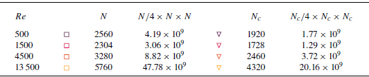
, respectively. The computational domain is discretised with
 $(N_x,N_y,N_z) = (640,2560,2560)$
for
 $Re=500$
,
 $(N_x,N_y,N_z)=(576,2304,2304)$
for
 $Re=1500$
,
 $(N_x,N_y,N_z) = (820,3280,3280)$
for
 $Re=4500$
and
 $(N_x,N_y,N_z) = (1440,5760,5760)$
for
 $Re=13\,500$
, for a total of more than
 $47\times 10^9$
grid points for the largest
 $Re$
considered. The distribution of points is uniform in the three directions with a grid spacing of
 $\Delta x = \Delta y = \Delta z \approx 0.039h$
for
 $Re=500$
and
 $Re=1500$
and of
 $0.0244h$
and
 $0.0121h$
for
 $Re=4500$
and
 $Re=13\,500$
, which leads to
 $26$
,
 $26$
,
 $41$
and
 $83$
grid points placed along the inlet slit, respectively. Grid resolution adequacy was verified by ensuring that the grid spacing is of the order of the local Kolmogorov scale, with
 $\eta _k/\varDelta \approx 1$
throughout the spreading region of the jet, see figure 19. For each Reynolds number, we have carried out an additional simulation on a coarser grid by reducing the number of points by a factor of approximately
 $0.75$
in the three directions, and observed only a marginal variation of the results; for more details on the convergence studies with respect to the grid spacing, we refer the reader to Appendix A. The time step has been fixed to a value of
 $\Delta t = 10^{-3} h/V_0$
for all cases, to ensure that the Courant–Friedrichs–Lewy number remains well below unity. After reaching statistical convergence, the four simulations are advanced for more than
 $1000 h/V_0$
(
 $Re=500$
),
 $800 h/V_0$
(
 $Re=1500$
),
 ${1065} h/V_0$
(
 $Re=4500$
),
 ${715} h/V_0$
(
 $Re=13\,500$
) time units to collect the flow statistics. Details of the numerical simulations are summarised in table 1.
Summary of the simulated cases. The colour code shown in the left-hand column is adopted throughout the work.

In the following, if not otherwise indicated, all quantities are made dimensionless with
 $V_0$
and
 $h$
. The classical Reynolds decomposition is used, i.e.
 $\{\boldsymbol{u},p\} = \{\boldsymbol{U}, P\} + \{\boldsymbol{u}',p'\}$
, with
 $\boldsymbol{U}=\langle \boldsymbol{u} \rangle$
and
 $P=\langle p \rangle$
, where the operator
 $\langle \cdot \rangle$
indicates averaging in time, along the spanwise homogeneous direction, and over the top and bottom halves of the jet (due to symmetry), while the prime
 $\cdot '$
indicates the fluctuating component.
3. Results
3.1. Inlet flow characterisation
In this section, we use instantaneous snapshots to illustrate the development of the jet from the potential core region at the inlet to the far-field region. The focus is on the effect of the inlet Reynolds number on the structures of the flow, and on the transition to turbulence. We use the
 $\lambda _2$
criterion, that has been proved to be an effective criterion to identify coherent structures in different configurations (Jeong & Hussain Reference Jeong and Hussain1995).
Figure 1 highlights that the flow close to the inlet is laminar and two-dimensional. The
 $\lambda _2$
isosurfaces show that the flow is smooth until pairs of spanwise aligned vortices appear due to the KH instability. The positions of the first appearance of the KH instability moves upstream as the Reynolds number is increased, being
 $y \approx 17h$
for
 $Re=500$
,
 $y \approx 7h$
for
 $Re=1500$
,
 $y \approx 3h$
for
 $Re=4500$
and
 $y \approx 2h$
for
 $Re=13\,500$
. When comparing with the experimental and numerical works found in the literature (see for example Da Silva & Métais Reference Da Silva and Métais2002 and Stanley et al. Reference Stanley, Sarkar and Mellado2002), our results predict that the flow becomes unstable at larger distances from the inlet, as we do not add any disturbance at the inlet to induce an earlier flow transition. Moving farther downstream, the KH rolls are deformed and modulated along the spanwise direction under the action of the velocity gradients, promoting thus a quick transition to turbulence. They first roll-up forming hairpin-like structures, and then break down into smaller and smaller scales. At intermediate distances, the large-scale structures that result from the flow instabilities coexist with the small-scale turbulent structures, whereas in the downstream self-similar region the flow is dominated by the small scales only, especially at high Reynolds numbers. Moving downstream, the vertical spreading of the jet in the vertical direction is clearly visible, especially for the largest Reynolds numbers considered, i.e.
 $Re=4500$
and
 $13\,500$
. The lateral view clearly shows that, as the inlet Reynolds number increases, the overall flapping motion of the jet decreases and the flow becomes progressively more dominated by the small scales of turbulence. Note also that the intensity of the vorticity at each
 $y$
position becomes larger as the Reynolds number increases, with the flow structures becoming smaller and smaller.
The inlet Reynolds number clearly influences the early stage of the flow instabilities. At small
 $Re$
, the KH vortices along the top and bottom shear layers exhibit an asymmetric arrangement, which is consistent with the growth of a sinusoidal mode. At large
 $Re$
, instead, the KH vortices are symmetric with respect to the centreline, showing the amplification of a varicose mode. Notably, both modes are amplified for intermediate
 $Re$
, and a clear arrangement of the KH vortices is not visible. The existence of the symmetric and asymmetric modes has been well documented in previous experimental (Sato Reference Sato1960; Beavers & Wilson Reference Beavers and Wilson1970; Wygnanski & Gutmark Reference Wygnanski and Gutmark1971; Antonia et al. Reference Antonia, Browne, Rajagopalan and Chambers1983; Thomas & Goldschmidt Reference Thomas and Goldschmidt1986; Deo et al. Reference Deo, Mi and Nathan2008) and numerical (Stanley et al. Reference Stanley, Sarkar and Mellado2002) studies. The presence of the two modes can also be detected with the temporal energy spectra: as shown by Sato (Reference Sato1960), indeed, the passage frequency of the KH vortices is lower for the antisymmetric mode than for the symmetric one. In figure 2, we show the temporal energy spectra computed along the centreline at
 $(x,y,z) = (0,0.15L_y,0)$
. As anticipated, the spectrum shows a distinct peak at
 $f \approx 0.04 h/V_0$
for
 $Re=500$
, while the energy spectrum peaks at approximately twice the frequency for
 $Re=13\,500$
, i.e. at
 $f \approx 0.105 h/V_0$
, values that are close to the frequencies detected in the experiments by Deo et al. (Reference Deo, Mi and Nathan2008). Instead, no clear peak is observed in the energy spectrum for
 $Re=1500$
, suggesting that the two modes interact giving rise to a wider range of frequencies at intermediate
 $Re$
.
Temporal spectra of the energy, for different Reynolds numbers, computed from probes located at the centreline at
 $y=0.15L_y$
; data is shifted upwards for ease of reading. The vertical dashed lines highlight the dominant frequency near the inlet (asymmetric mode, low frequency peak – symmetric mode, high frequency peak, see Deo et al. Reference Deo, Mi and Nathan2008).

 $(a)$
Dependence of the centreline velocity
 $V_c$
on
 $Re$
; the power law scaling
 $V_c/V_0\propto (y/h)^{-1/2}$
is reported with a black dashed line.
 $(b)$
Reynolds-dependence of the slope
 $\alpha _{V_c}$
, such that
 $(V_o/V_c)^2 = \alpha _{V_c} y/h$
. In panel
 $(b)$
, data from previous experimental works are also reported for comparison, i.e. DMN-2008a (Deo et al. Reference Deo, Mi and Nathan2008, with nozzle aspect ratio of
 ) DMN-2008b (Deo et al. Reference Deo, Mi and Nathan2008, with
 ) DMN-2008c (Deo et al. Reference Deo, Mi and Nathan2008, with
 ) NO-1988 (Namer & Ötügen Reference Namer and Ötügen1988 with (
 )) and SSSD-2008 (Suresh et al. Reference Suresh, Srinivasan, Sundararajan and Das2008 width
 ).

3.2. Mean flow statistics
We now move onto the effect of the Reynolds number on the bulk statistics of the planar jet.
In terms of mean-field quantities, the spatial evolution of a jet can be described by looking at the centreline velocity
 $V_c$
and at the jet thickness
 $\delta _{0.5}$
. The centreline velocity
 $V_c$
, defined as the time and space (
 $x$
) average of the streamwise velocity at the jet centreline
 $V_c(y)= V(y,0)$
, is reported in figure 3
 $(a)$
. The centreline velocity shows a non-monotonic behaviour for increasing values of the Reynolds number. At low Reynolds numbers (
 $Re \leqslant 1500$
), the decay of the centreline velocity is low up to approximately
 $60h$
, and only then a sharp reduction in the centreline velocity is reported. As seen in figure 1, the flow at the lowest value of the Reynolds number is characterised by large, coherent and quasi-two-dimensional spanwise structures up to approximately
 $y/h\approx 50$
, that merge and decay only away from the inlet, causing the sharp decay observed in the centreline velocity. The centreline velocity at
 $Re=1500$
shows the largest decay rate for all cases, due to the coexistence of large spanwise vortices and small turbulent structures, the former providing large-scale mixing and the latter small-scale mixing. For larger values of the Reynolds number
 $Re\geqslant 4500$
, the centreline velocity shows the smallest decay rate: here, the large-scale spanwise vortices are quickly dissipated close to the inlet, and both
 $Re=4500$
and
 $Re=13\,500$
show similar values of the centreline velocity at all
 $y$
, suggesting that the value of the centreline velocity of a planar jet becomes independent of the Reynolds number for
 $Re\gtrsim 4500$
. Figure 3
 $(a)$
clearly shows the presence of the expected power law scaling
 $V_c \propto y^{-1/2}$
(Bradbury Reference Bradbury1965; Pope Reference Pope2000) for the larger Reynolds numbers for
 $y/h\geqslant 20$
. For the cases at lower Reynolds number, instead, a power law scaling steeper than
 $-1/2$
is reported. Linear regression has been performed to infer the value of the slope
 $\alpha _{V_c}$
, such that
 $(V_0/V_c)^2=\alpha _{V_c} y/h$
. For the linear regression, we set the power law scaling to
 $V_c \propto y^{-1/2}$
for all values of
 $Re$
; this is done in order to compare our data with the experimental results from Suresh et al. (Reference Suresh, Srinivasan, Sundararajan and Das2008), where this power law exponent was used for Reynolds numbers as low as
 $Re=250$
. Linear regression was performed over a range of streamwise coordinate where the derivative of
 $(V_0/V_c)^2$
fluctuates around a constant value. The dependence of the slope
 $\alpha _{V_c}$
on the Reynolds number is shown in figure 3
 $(b)$
, together with data from experiments (Namer & Ötügen Reference Namer and Ötügen1988; Deo et al. Reference Deo, Mi and Nathan2008; Suresh et al. Reference Suresh, Srinivasan, Sundararajan and Das2008). In agreement with the results from previous studies, we find a decreasing trend of
 $\alpha _{V_c}$
for increasing values of the Reynolds number (the first point at
 $Re=500$
shows a different behaviour due to the different level of noise at the inlet between the simulations and experiments). According to the experimental data, the value of the slope
 $\alpha _{V_c}$
becomes almost independent of the Reynolds number for
 $Re\gtrsim 4500$
, and our simulations at the larger
 $Re$
confirm the trend.
 $(a)$
Dependence of the streamwise evolution of the jet thickness
 $\delta _{0.5}/h$
on
 $Re$
; the scaling
 $\delta _{0.5}/h \propto y/h$
is reported with a black dashed line. The inset shows the ratio
 $\delta _{mom}/\delta _{0.5}$
for different
 $Re$
.
 $(b)$
Dependence of the slope
 $\alpha _{\delta _{0.5}}$
such that
 $\delta _{0.5} = \alpha _{\delta _{0.5}} y/h$
on
 $Re$
. In panel
 $(b)$
data from previous experimental works are also reported for comparison, i.e. DMN-2008c (Deo et al. Reference Deo, Mi and Nathan2008, with
 ) NO-1988 (Namer & Ötügen Reference Namer and Ötügen1988 with
 ) and SSSD-2008 (Suresh et al. Reference Suresh, Srinivasan, Sundararajan and Das2008 with
 ).

The jet thickness
 $\delta _{0.5}$
, defined as the distance from the centreline at which the mean streamwise velocity equals half the centreline velocity
 $V(y,\delta _{0.5}(y))=0.5V_c(y)$
, is reported in figure 4
 $(a)$
. Similarly to what is observed for the centreline velocity, the jet thickness exhibits a non-monotonic trend with the Reynolds number. At the lowest value, the jet has the lowest spreading rate up to around
 $50h$
, while beyond this streamwise position a sharp increase of the jet thickness is observed. This change in the spreading rate of the jet is consistent with the roll-up of the large, quasi-two-dimensional spanwise vortices previously mentioned. At the intermediate Reynolds number,
 $Re=1500$
, we observe a similar transition at
 $y \approx 50h$
, but with an initial larger spreading rate. Finally, at the high Reynolds numbers,
 $Re \geqslant 4500$
, the jet widens at a constant rate. We perform a linear regression of the jet thickness, in a range of streamwise coordinates where the growth rate of the jet fluctuates about a constant value as well. For all values of the Reynolds number, we observe a linear growth of the jet thickness with the streamwise coordinate, which agrees with the linear scaling
 $\delta _{0.5} \propto y$
reported in previous works (Bradbury Reference Bradbury1965; Gutmark & Wygnanski Reference Gutmark and Wygnanski1976; Pope Reference Pope2000). In figure 4
 $(b)$
, we report the growth rate coefficient
 $\alpha _{\delta _{0.5}}$
of the linear scaling
 $\delta _{0.5}=\alpha _{\delta _{0.5}} y$
, and observe a good agreement with previous experimental data for
 $Re\geqslant 1500$
; at the lowest Reynolds number the measured spreading rate is instead much smaller than the experimental value, as also observed for the centreline velocity. The spreading rate of the jet reduces with increasing values of the Reynolds number and achieves an approximately constant value
 $\alpha _{\delta _{0.5}}\approx 0.08$
at high Reynolds number (
 $Re\gtrsim 4500$
), consistent with past experimental works (Bradbury Reference Bradbury1965; Heskestad Reference Heskestad1965; Gutmark & Wygnanski Reference Gutmark and Wygnanski1976; Pope Reference Pope2000; Deo et al. Reference Deo, Mi and Nathan2008). We include also an alternative definition of the jet thickness, the momentum thickness
 $\delta _{mom}$
, which has been adopted in previous works on planar jets (Guimarães et al. Reference Guimarães, Pimentel, Pinho and da Silva2020). The momentum thickness
 $\delta _{mom}$
is defined as the half-thickness of an inviscid, shearless jet carrying the same flow rate and with velocity equal to the centreline velocity, i.e.
 \begin{equation} \delta _{mom}=\frac {1}{2} \frac {\int _{-L_z/2}^{L_z/2} V {{\textrm d}}z}{V_c} \, . \end{equation}
In the inset of figure 4
 $(a)$
we report the ratio
 $\delta _{mom}/\delta _{0.5}$
to provide a quantitative comparison between the two definitions. The ratio fluctuates around unity for all cases, converging towards one for large-enough Reynolds numbers and away from the inlet. In the following we use the jet thickness
 $\delta _{0.5}$
as the reference jet thickness.
The effect of the Reynolds number on the self-similar profile of the (a,c,e,g) streamwise and (b,d,f,h) jet-normal velocity components. Each row corresponds to a different Reynolds number: panels
 $(a)$
and
 $(b)$
are for
 $Re=500$
; panels
 $(c)$
and
 $(d)$
are for
 $Re=1500$
; panels
 $(e)$
and
 $(f)$
are for
 $Re=4500$
; panels
 $(g)$
and
 $(h)$
are for
 $Re=13\,500$
. Each curve is averaged over a range of
 $5h$
around the chosen streamwise position. Markers report data from previous experiments and simulations: downward triangles are for Bradbury (Reference Bradbury1965), squares for Namer & Ötügen (Reference Namer and Ötügen1988), diamonds for Stanley et al. (Reference Stanley, Sarkar and Mellado2002), circles for Deo et al. (Reference Deo, Mi and Nathan2008), stars for Suresh et al. (Reference Suresh, Srinivasan, Sundararajan and Das2008), upward triangles for Cafiero & Vassilicos (Reference Cafiero and Vassilicos2019). The black dashed line corresponds to the analytic solution obtained under the hypothesis of uniform turbulent viscosity.

The streamwise and jet-normal velocity profiles are reported in figure 5 at several streamwise locations, starting from
 $y/h=40$
from where self-similarity is commonly observed (Bradbury Reference Bradbury1965; Heskestad Reference Heskestad1965; Gutmark & Wygnanski Reference Gutmark and Wygnanski1976). Here, the data are averaged over a streamwise distance of
 $\pm 2.5h$
from the indicated streamwise position (after being normalised by the local centreline velocity
 $V_c$
and reported against the normalised jet-normal coordinate
 $z/\delta _{0.5}$
), thus exploiting the self-similarity of the jet flows at high (Bradbury Reference Bradbury1965; Heskestad Reference Heskestad1965) Reynolds numbers. Velocity profiles at the lower Reynolds numbers (
 $Re = 500$
and
 $Re=1500$
) are also shown for comparison, although these cases do not exhibit a fully developed self-similar regime with the classical
 $(V_0/V_c)^2 \sim y/h$
scaling. Figure 5 also includes experimental (Bradbury Reference Bradbury1965; Namer & Ötügen Reference Namer and Ötügen1988; Deo et al. Reference Deo, Mi and Nathan2008; Suresh et al. Reference Suresh, Srinivasan, Sundararajan and Das2008; Cafiero & Vassilicos Reference Cafiero and Vassilicos2019) and numerical (Stanley et al. Reference Stanley, Sarkar and Mellado2002) results found in the literature at comparable
 $Re$
, together with the analytic profile of the streamwise velocity obtained under the hypothesis of uniform turbulent viscosity, i.e.
 $v/V_c=1/\cosh ^2{(c\,z/\delta _{0.5})}$
with
 $c=0.5 \ln {(1+\sqrt {2})^2}\approx 0.88$
(Pope Reference Pope2000). Note that, as shown in the following, the hypothesis of uniform turbulent viscosity holds only in the core of the jet, approximately up to one jet thickness from the centreline, i.e. up to
 $z\simeq \delta _{0.5}$
. For the streamwise velocity component shown in figure 5(a,c,e,g), we observe a good agreement between the present dataset, the analytic profile, and previous numerical and experimental measurements. At low Reynolds numbers,
 $Re=500$
and
 $Re=1500$
, there is a clear residual effect of the streamwise position, with the profiles departing from the experimental values for increasing distances from the inlet, indicating a lack of full self-similarity. For larger
 $Re$
, instead, the velocity profiles become clearly self-similar, as indicated by the good overlap of the profiles at different streamwise positions. An excellent agreement with previous experimental and simulation data and with the analytic profile is also evident. Similarly, for the jet-normal velocity component we observe self-similarity for
 $Re \geqslant 4500$
only; see figure 5(b,d,f,h). Again, good agreement is observed with the simulation data of Stanley et al. (Reference Stanley, Sarkar and Mellado2002) at
 $Re=3000$
and with the simulation data of Bradbury (Reference Bradbury1965), whereas some discrepancies are found with the measurements of Cafiero & Vassilicos (Reference Cafiero and Vassilicos2019), which exhibit a peak closer to the centreline and a faster decay moving away from the centreline. Note also the non-monotonic trend in the intensity of the jet-normal velocity for increasing values of the Reynolds number, which is largest at
 $Re=1500$
, with a peak value of around
 $W\approx 0.075V_c$
, and decreases for larger Reynolds numbers, converging towards a peak value of
 $W\approx 0.018V_c$
.
Dependence of the length of the potential core on
 $Re$
.
 $(a)$
Length of the potential core as a function of the Reynolds number, Panels
 $(b)$
and
 $(c)$
provide close-up views at the inlet of the centreline velocity and TKE, used for the definitions of
 $l_{c,V_c}$
and
 $l_{c,\textit{TKE}}$
. In panel
 $(a)$
data from Deo et al. (Reference Deo, Mi and Nathan2008) are also reported for comparison; in their work, the length of the potential core was defined based on the 98 % of the centreline velocity.

We conclude this section by looking at the near-inlet region. Close to the inlet, in the so-called potential core, the flow has an almost constant centreline velocity and jet thickness. The length of the potential core is commonly defined by looking at the distance from the inlet at which the centreline velocity is equal to 98 % of the centreline velocity at the inlet; see
 $l_{c,V_c}$
in figure 6
 $(a)$
. We report as well the experimental data of Deo et al. (Reference Deo, Mi and Nathan2008), based on the 98 % centreline velocity method. We observe a slight non-monotonic behaviour in the potential core length for increasing values of
 $Re$
: indeed, the potential core length increases with the Reynolds number between
 $Re=500$
and
 $Re=1500$
, and then starts decreasing beyond
 $Re\geqslant 1500$
. The effect of different thresholds on the potential core length is tested via the error bars in figure 6
 $(a)$
(top,
 $0.97V_0$
; bottom,
 $0.99V_0$
), showing that the trend with the Reynolds number is overall robust. Figure 6
 $(b)$
shows a magnification of the centreline velocity within the potential core of the jet, together with the three threshold values selected to identify the length of the potential core (dashed lines). At high Reynolds number,
 $Re\geqslant 4500$
, the centreline velocity exhibits small fluctuations near the inlet due to the destabilisation of the stream and transition to turbulence. These fluctuations evolve very slowly in time and thus require averaging over very long time periods. To remedy to the effect of these long-lived fluctuations in the centreline velocity on the potential core length, we adopt an alternative definition based on the TKE sampled at the centreline,
 $q = (\langle u^{\prime}u^{\prime}\rangle +\langle v^{\prime}v^{\prime} \rangle +\langle w^{\prime}w^{\prime} \rangle )|_{z=0}/2$
(see e.g. Browne, Antonia & Chambers Reference Browne, Antonia and Chambers1984). The TKE, shown in figure 6
 $(c)$
, is zero at the inlet and rapidly grows within
 $20h$
from the inlet, reaching its peak value (not shown here) within around
 $40h$
. The departure from zero TKE moves closer to the inlet for increasing values of the Reynolds number, in agreement with the early transition to turbulence reported in § 3.1. To identify the potential core length based on the TKE, we set a threshold value equal to
 $10^{-3}$
, shown with a dashed black line in figure 6
 $(c)$
; note that, the selected threshold value corresponds to approximately 1 % of the peak value. To test the dependence of the potential core length on the selected threshold, two additional values, twice and half the original value, are also considered (grey dashed lines). The potential core length based on the TKE threshold,
 $l_{c,\textit{TKE}}$
, is also shown in figure 6
 $(a)$
, with the error bars showing the effect of the different threshold values. The length of the potential core
 $l_{c,\textit{TKE}}$
shows a monotonic decrease in the potential core length for increasing Reynolds number, in agreement with the experimental data of Deo et al. (Reference Deo, Mi and Nathan2008), with a value only slightly dependent of the selected threshold. Thus, the latter definition of the potential core length appears to be more robust compared with the original based on the centreline velocity, with the TKE signal not showing any significant fluctuation near the inlet.
3.3. Turbulent statistics in the core of the jet
We now move to the fluctuating velocity field, and start focusing on the Reynolds stresses
 $\langle u^{\prime}_i u^{\prime}_j \rangle$
. Due to the symmetries of the flow, the only non-zero shear stress is
 $\langle v^{\prime}w^{\prime} \rangle$
. Also, it is well known (Pope Reference Pope2000) that, for large enough Reynolds number and after the development region,
 $u^{\prime}_{i,rms}|_{z=0} \equiv \langle u^{\prime}_i u^{\prime}_i \rangle ^{1/2}|_{z=0}$
decays with the same power law as the centreline velocity, i.e.
 $ \langle u^{\prime}_i u^{\prime}_i \rangle |_{z=0} \sim V_c^2 \sim y^{-1}$
, and that the jet-normal profiles of
 $\langle u^{\prime}_i u^{\prime}_j \rangle$
are self-similar.
Streamwise evolution for different Reynolds number of the three diagonal components of the Reynolds stress tensor, normalised by the centreline velocity:
 $(a)$
 $ \langle u^{\prime}u^{\prime} \rangle$
;
 $(b)$
 $ \langle v^{\prime}v^{\prime} \rangle$
;
 $(c)$
 $\ \langle w^{\prime}w^{\prime} \rangle$
.

Figure 7 shows the downstream evolution of the three normal stresses along the jet centreline, normalised by the centreline velocity, such that the self-similar region starts when
 $\langle u^{\prime}_i u^{\prime}_i \rangle /V_c^2|_{z=0}$
approaches a constant value. For all the Reynolds numbers, the intensity of the fluctuations is substantially zero in the potential core, and then quickly increases when transitioning to turbulence, where it shows a localised peak, before decreasing again. Compared with previous studies, our data show a more pronounced peak in the development region, see for example figure 11 by Stanley et al. (Reference Stanley, Sarkar and Mellado2002) (planar jet at
 $Re=3000$
) and figures 7–10 by Nguyen & Oberlack (Reference Nguyen and Oberlack2024) (round jet at
 $Re=3500$
). We believe that the difference is linked to the absence of noise at the inlet in our simulations, which has been instead applied in previous works to accelerate the transition to turbulence. We observe that the fluctuations do not exhibit self-similarity for
 $Re \leqslant 1500$
. Notably,
 $\langle u^{\prime}u^{\prime} \rangle |_{z=0} \approx 0$
up to
 $y \approx 60h$
for
 $Re=500$
, and up to
 $y \approx 30h$
for
 $Re=1500$
, indicating a substantially two-dimensional flow. For larger
 $Re$
, instead, the normalised normal stresses
 $\langle u^{\prime}_i u^{\prime}_i \rangle /V_c^2$
approach a constant value, that only marginally changes between
 $Re=4500$
and
 $Re=13\,500$
, suggesting that in the self-similar region the profiles of
 $\langle u_i u_j\rangle /V_c^2$
lose the dependence on the Reynolds number for
 $Re \gtrapprox 4500$
. Our data show that
 $\langle v^{\prime}v^{\prime} \rangle /V_c^2|_{z=0}$
and
 $\langle w^{\prime}w^{\prime}\rangle /V_c^2|_{z=0}$
reach a plateau for
 $y \gtrapprox 40h$
, while
 $\langle u^{\prime}u^{\prime} \rangle /V_c^2|_{z=0}$
approaches a constant value only at larger
 $y/h$
, in agreement with the numerical results of Stanley et al. (Reference Stanley, Sarkar and Mellado2002). In the self-similar region, we measure
 $\langle v^{\prime}v^{\prime} \rangle \approx 0.052 /V_c^2|_{z=0}$
, which corresponds to
 $v^{\prime}_{rms} \approx 0.228 V_c|_{z=0}$
, thus resulting in the root mean square of the streamwise velocity fluctuations being approximately
 $23\, \%$
of the mean velocity at the jet centreline. This value is comparable to what found by previous numerical and experimental studies; for example, Stanley et al. (Reference Stanley, Sarkar and Mellado2002) report
 $v^{\prime}_{rms} \approx 0.25 V_c|_{z=0}$
at
 $Re=3000$
, while Thomas & Chu (Reference Thomas and Chu1989) and Thomas & Prakash (Reference Thomas and Prakash1991) measured
 $v^{\prime}_{rms} \approx 0.23 V_c|_{z=0}$
at
 $Re \approx 7000{-}8000$
. For completeness, we mention that Hussein, Capp & George (Reference Hussein, Capp and George1994) reported a value of
 $v^{\prime}_{rms} \approx 0.25 V_c|_{z=0}$
for round jets. In agreement with the anisotropy of the flow, the intensity of the cross-stream fluctuations is smaller, with
 $u^{\prime}_{rms} \approx 0.19 /V_c|_{z=0}$
(
 $\approx \sqrt {0.036}$
) and
 $w^{\prime}_{rms} \approx 0.2 /V_c|_{z=0}$
(
 $\approx \sqrt {0.039}$
) (see also, Stanley et al. Reference Stanley, Sarkar and Mellado2002 and Nguyen & Oberlack Reference Nguyen and Oberlack2024).
Profiles of the Reynolds stresses in the self-similar region:
 $(a)$
 $ \langle u^{\prime}u^{\prime} \rangle$
;
 $(b)$
 $ \langle v^{\prime}v^{\prime} \rangle$
;
 $(c)$
 $ \langle w^{\prime}w^{\prime} \rangle$
;
 $(d)$
 $ \langle v^{\prime}w^{\prime} \rangle$
. Symbols refer to literature data: squares (Gutmark & Wygnanski Reference Gutmark and Wygnanski1976), circles (Ramaprian & Chandrasekhara Reference Ramaprian and Chandrasekhara1985), diamonds (Thomas & Prakash Reference Thomas and Prakash1991), downwards triangles (Stanley et al. Reference Stanley, Sarkar and Mellado2002).

Figure 8 shows the profiles of the Reynolds stress components in the self-similar region for
 $Re=4500$
and
 $Re=13\,500$
, while the profiles at the lower Reynolds numbers are not reported here due to the absence of self-similarity. These profiles are obtained after averaging in time, along the spanwise direction, and along the streamwise direction within the self-similar region over a distance of
 $20h$
in the streamwise direction. We take advantage of the top–bottom symmetry: data from the top-half (above centreplane,
 $z\geqslant 0$
) and from the bottom-half (below centreplane,
 $z\lt 0$
) of the domain are averaged together to double the statistical sample. We observe minor differences between the two considered Reynolds numbers, suggesting that (like the mean-flow statistics) the self-similar Reynolds stresses become independent of the Reynolds number only for
 $Re \gtrapprox 4500$
. Although the data in the literature are rather scattered, we find a fair collapse with other numerical (Stanley et al. Reference Stanley, Sarkar and Mellado2002) and experimental (Gutmark & Wygnanski Reference Gutmark and Wygnanski1976; Ramaprian & Chandrasekhara Reference Ramaprian and Chandrasekhara1985; Thomas & Prakash Reference Thomas and Prakash1991) studies at different Reynolds numbers. Note that the numerical data of Stanley et al. (Reference Stanley, Sarkar and Mellado2002) predicts a larger
 $\langle w^{\prime}w^{\prime} \rangle$
as a result of the forcing they use at the inlet to accelerate the transition to turbulence, as also mentioned by the authors.
Streamwise evolution of the three normal stresses normalised with the TKE at
 $z = \delta _{0.5}$
: (a)
 $Re=500$
; (b)
 $Re=1500$
; (c)
 $Re=4500$
; (d)
 $Re=13\,500$
.

We now focus on the shear layers that separate the turbulent and non-turbulent regions, and investigate how the velocity fluctuations are organised there at the different stages of the jet development; this is the region where the intensity of the fluctuations is maximum. Figure 9 plots the streamwise evolution of the three normal stresses at
 $z = \delta _{0.5}$
, normalised with the local TKE, i.e.
 $\langle u^{\prime}_i u^{\prime}_i \rangle /q|_{\delta _{0.5}}$
. The near-inlet region where
 $\langle w^{\prime}w^{\prime} \rangle \approx \langle u^{\prime}u^{\prime} \rangle \approx 0$
and
 $\langle v^{\prime}v^{\prime} \rangle \approx 2q$
corresponds to the potential core; here the fluctuating kinetic energy is substantially null (see figure 6) and entirely contained in the streamwise component. Moving downstream, the partition of TKE in the three components depends on the Reynolds number. For small
 $Re \leqslant 1500$
, the shear layer is dominated by
 $\langle v^{\prime}v^{\prime} \rangle$
and
 $\langle w^{\prime}w^{\prime} \rangle$
, with
 $\langle v^{\prime}v^{\prime} \rangle \approx \langle w^{\prime}w^{\prime} \rangle \approx q$
and
 $\langle u^{\prime} u^{\prime} \rangle \approx 0$
(except close to the outlet where
 $\langle w^{\prime}w^{\prime} \rangle \gt \langle v^{\prime}v^{\prime} \rangle$
). This is consistent with the presence of large two-dimensional structures that induce intense streamwise and vertical fluctuations at their sides (see figure 1). The scenario changes for
 $Re \geqslant 4500$
, in agreement with the quicker dissipation of the large-scale coherent vortices. In the region immediately downstream the potential core, the fluctuating energy is dominated by the vertical contribution, with
 $\langle w^{\prime}w^{\prime} \rangle \approx 1.5q$
; this is again the statistical trace of the KH rolls. In contrast, in the downstream self-similar region, we find that
 $ \langle v^{\prime}v^{\prime} \rangle \approx 0.75q$
and
 $ \langle u^{\prime}u^{\prime} \rangle \approx \langle w^{\prime}w^{\prime} \rangle \approx 0.625q$
. The fact that
 $\langle v^{\prime}v^{\prime} \rangle \gt \langle u^{\prime}u^{\prime} \rangle \approx \langle w^{\prime}w^{\prime} \rangle$
is consistent with the strong anistropy induced by the mean shear, where the streamwise velocity fluctuations are fed by the production term
 $P_{22} \approx - 2 \langle v^{\prime}w^{\prime} \rangle \partial V/\partial z$
, while the cross-stream ones are mainly sustained by the redistributive action of the pressure; see the following discussion. To quantify the flow anisotropy, we report in table 2 the values of
 $ \langle u^{\prime}u^{\prime} \rangle /q$
,
 $ \langle v^{\prime}v^{\prime} \rangle /q$
,
 $ \langle w^{\prime}w^{\prime} \rangle /q$
and
 $ \langle u^{\prime}v^{\prime} \rangle /q$
for
 $Re=13\,500$
at different values of
 $z/\delta _{0.5}$
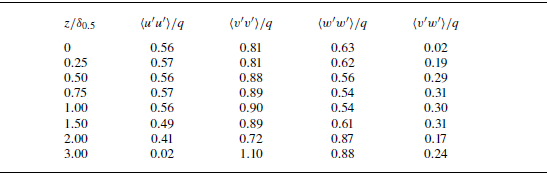
. We start looking at the shear stress as a proxy of the flow anisotropy:
 $ \langle v^{\prime}w^{\prime} \rangle /q$
is null at the jet centreline, and plateaus in the bulk of the jet, where exhibits a value of
 $ \langle v^{\prime}w^{\prime} \rangle \approx 0.28q-0.3q$
, which agrees reasonably well with the value reported by Stanley et al. (Reference Stanley, Sarkar and Mellado2002) and is close to the experimental value found in turbulent shear layers (see for example Spencer & Jones Reference Spencer and Jones1971 and Bell & Mehta Reference Bell and Mehta1990). Thus, the flow anisotropy is minimum at the centreline, where
 $ \langle u^{\prime}u^{\prime} \rangle / \langle v^{\prime}v^{\prime} \rangle \approx 0.69$
and
 $ \langle w^{\prime}w^{\prime} \rangle / \langle v^{\prime}v^{\prime} \rangle \approx 0.77$
. At
 $z \approx \delta _{0.5}$
there is a substantial balance between the cross-stream components, with
 $ \langle u^{\prime}u^{\prime} \rangle / \langle v^{\prime}v^{\prime} \rangle \approx 0.63$
and
 $ \langle w^{\prime}w^{\prime} \rangle / \langle v^{\prime}v^{\prime} \rangle \approx 0.63$
, while the spanwise fluctuations quickly decrease for
 $z \gt \delta _{0.5}$
, with the vertical component growing and becoming comparable to the streamwise one. At
 $z \approx 3 \delta _{0.5}$
, we indeed find
 $ \langle u^{\prime}u^{\prime} \rangle / \langle v^{\prime}v^{\prime} \rangle \approx 0.02$
and
 $ \langle w^{\prime}w^{\prime} \rangle / \langle v^{\prime}v^{\prime} \rangle \approx 0.8$
.
Jet anisotropy in the self-similar region for
 $Re=13\,500$
. Note that for
 $z/\delta _{0.5}=0$
 $ \langle v^{\prime}w^{\prime} \rangle /q \rightarrow 0$
when increasing the integration time.

Besides the flow anisotropy, the knowledge of the spatial distribution of the Reynolds stresses is important from the modelling viewpoint. Due to the symmetries of the flow, in the present configuration the shear stress
 $ \langle v^{\prime}w^{\prime} \rangle$
goes to zero where
 $\partial V / \partial z = 0$
and it is negative where
 $\partial V/\partial z$
is positive. This means that one may define a positive turbulent viscosity
 $\nu _T$
such that
 $ \langle u^{\prime}w^{\prime} \rangle = - \nu _T \partial V/\partial z$
(Pope Reference Pope2000); the knowledge of the spatial distribution of
 $\nu _T$
is of paramount importance for modelling, as it permits us to overcome the closure problem of the Reynolds-averaged Navier–Stokes equations. Following the behaviour of the Reynolds stresses and of the mean velocity, also
 $\nu _T$
is expected to exhibit self-similarity in the developed region of the jet. In other words the profiles of
 $\nu _T/V_c \delta _{0.5}$
are expected to be a function of
 $z/\delta _{0.5}$
only. We find that
 $\nu _T/V_c \delta _{0.5}$
is approximately uniform in the bulk of the jet flow for
 $Re \geqslant 4500$
(see figure 10), and decays to zero moving away from the jet centreline, similarly to the results reported by Hussein et al. (Reference Hussein, Capp and George1994) for round jets. We observe a fairly good agreement between the value measured for
 $Re = 4500$
and
 $Re = 13\,500$
: we measure an average value of
 $ \langle \nu _T \rangle \approx 0.046 V_c \delta _{0.5}$
and
 $0.040 V_c \delta _{0.5}$
in the
 $0.3 \leqslant z/\delta _{0.5} \leqslant 1$
range. We mention that our estimate of
 $\nu _T$
is larger than the value of
 $0.035 V_c \delta _{0.5}$
found by Hussein et al. (Reference Hussein, Capp and George1994) for a round jet, and the value of
 $0.032 V_c \delta _{0.5}$
reported by Pope (Reference Pope2000) for a planar jet.
Profiles of the turbulent viscosity in the self-similar regime for
 $Re=4500$
and
 $Re=13\,500$
.

Evolution of the dissipation rate of the TKE along the centreline.

We now move to the budget equation for the Reynolds stresses which reads (Pope Reference Pope2000)
 \begin{equation} \begin{gathered} \underbrace {U_k \frac {\partial }{\partial x_k} \langle u^{\prime}_i u^{\prime}_j \rangle }_{A_{ij}} + \underbrace { \frac {\partial }{\partial x_k} ( \langle u^{\prime}_k u^{\prime}_i u^{\prime}_j \rangle + \langle p' u^{\prime}_j \rangle \delta _{ik} + \langle p' u^{\prime}_i \rangle \delta _{jk} - \nu \frac {\partial }{\partial x_k} \langle u^{\prime}_i u^{\prime}_j \rangle ) }_{T_{ij}} = \\[1pt] \underbrace { - \langle u^{\prime}_k u^{\prime}_i \rangle \frac {\partial U_j}{\partial x_k} - \langle u^{\prime}_k u^{\prime}_j \rangle \frac {\partial U_i}{\partial x_k} }_{P_{ij}} + \underbrace { \bigg\langle p' \frac {\partial u^{\prime}_i}{\partial x_k} \bigg\rangle + \bigg\langle p' \frac {\partial u^{\prime}_j}{\partial x_k} \bigg\rangle }_{\Pi _{ij}} - \underbrace { \nu \bigg\langle \frac {\partial u^{\prime}_i}{\partial x_k} \frac {\partial u^{\prime}_j}{\partial x_k } \bigg\rangle }_{\varepsilon _{ij}}. \end{gathered} \end{equation}
The terms on the left-hand side are the advection term
 $A_{ij}$
and the turbulent transport term
 $T_{ij}$
, which describe the transfers of the Reynolds stresses due to the action of the mean field and of the turbulent fluctuations, respectively. The right-hand side denotes the net sink/source regions for each component of the Reynolds stress tensor; the production term
 $P_{ij}$
describes the exchange of stresses between the mean and fluctuating fields, the pressure strain term
 $\Pi _{ij}$
couples the pressure with the fluctuating velocity derivatives and describes the redistribution of the TKE among the three normal stresses, and the pseudodissipation term
 $\varepsilon _{ij}$
describes the viscous dissipation of the Reynolds stresses. Summing together the terms on the right-hand side yields the net source term
 $\xi _{ij} = P_{ij} + \Pi _{ij} - \varepsilon _{ij}$
. Here we focus on the self-similar region of the jet, and thus consider only the
 $Re=4500$
and
 $Re=13\,500$
cases.
In the fully developed region the terms of (3.2) should decay as
 $\sim V_c^3 \delta _{0.5}^{-1} \sim y^{-5/2}$
and their profiles should become self-similar. Figure 11 shows the downstream evolution of the dissipation rate of the TKE, i.e.
 $\varepsilon /2$
where
 $\varepsilon \equiv \varepsilon _{ii}$
(here repeated indexes imply summation), made dimensionless with
 $V_c^3 \delta _{0.5}^{-1}$
, such that self-similarity is reached in the region where
 $-\varepsilon V_c^{-3} \delta _{0.5}^{-1}|_{z=0}$
approaches a constant value. Figure 11 shows that self-similarity is present for both the two largest Reynolds numbers, and the value at which
 $-\varepsilon V_c^{-3} \delta _{0.5}^{-1}$
plateaus appears to be the same for both cases, suggesting that it is
 $Re$
-independent for
 $Re \geqslant 4500$
. The plateau is reached at
 $y \gtrapprox 70h$
for
 $Re=4500$
, and at
 $y \gtrapprox 50h$
for
 $Re=13\,500$
.
Budget of
 $ \langle u^{\prime}u^{\prime} \rangle$
(a,b),
 $ \langle v^{\prime}v^{\prime} \rangle$
(c,d) and
 $ \langle w^{\prime}w^{\prime} \rangle$
(e,f) for
 $Re=4500$
(orange) and
 $Re=13\,500$
(red). Panels (a,c,e) are for the advection term
 $-A_{ij}$
, the turbulent transport term
 $-T_{ij}$
and the net source term
 $\xi _{ij}=P_{ij} + \Pi _{ij} - \varepsilon _{ij}$
. For clarity, here we consider only
 $Re=13\,500$
. Panels (b,d,f) detail the profiles of the production term
 $P_{ij}$
, the pressure strain
 $\Pi _{ij}$
and the pseudodissipation
 $ \langle \varepsilon _{ij} \rangle$
.

Figure 12 plots the terms of the budget equations for the three normal stresses (see (3.2)) in the self-similar region. The
 $A_{ij}$
,
 $P_{ij}$
,
 $\Pi _{ij}$
and
 $\varepsilon _{ij}$
terms have been computed at runtime while the simulations advance, while the turbulent transport term
 $T_{ij}$
has been evaluated a posteriori by enforcing the closure of (3.2). Figure 12 is obtained by averaging the profiles, once made dimensionless with the local values of
 $V_c$
and
 $\delta _{0.5}$
, in the
 $y/h \in (70,77)$
range for
 $Re=4500$
, and in the
 $y/h \in (55,65)$
range for
 $Re=13\,500$
. In figure 12(a,c,e) we show
 $-A_{ij}$
,
 $-T_{ij}$
and
 $\xi _{ij}$
for normal stresses, with the aim to identify the source and sink regions of the flow and highlight the role of the advection and turbulent transport terms. A positive (negative)
 $\xi _{ij}$
identifies a region of net source (sink) for
 $\langle u^{\prime}_i u^{\prime}_j \rangle$
. Positive (negative)
 $-A_{ij}$
and/or
 $-T_{ij}$
denote regions where the advection and/or turbulent transport term release (drain)
 $\langle u^{\prime}_i u^{\prime}_j \rangle$
. In other words,
 $\langle u^{\prime}_i u^{\prime}_j \rangle$
is transferred from the regions where
 $-A_{ij}$
and/or
 $-T_{ij}$
are negative to regions where they are positive. Figure 12(b,d,f) report separately the terms on the right-hand side of (3.2).
Figure 12(a,c,e) show that
 $\xi _{ij}\lt 0$
for
 $z/\delta _{0.5} \approx 0$
, while
 $\xi _{ij}\gt 0$
for
 $0.5 \lessapprox z/\delta _{0.5} \lessapprox 1.5$
; for
 $ \langle v^{\prime}v^{\prime} \rangle$
we also have that
 $\xi _{22}\lt 0$
for
 $z/\delta _{0.5} \gtrapprox 1.2$
. The sink regions of the flow are thus located at the centreline and at the edge of the jet, while the source region is confined at intermediate
 $z/\delta _{0.5}$
, where indeed the mean shear (and thus the production term) is maximum. In the sink region at the jet centreline, the velocity fluctuations are mainly sustained by the advection term
 $A_{ij}$
, which transfers
 $\langle u^{\prime}_i u^{\prime}_j \rangle$
from the edges of the jet towards the core; for
 $ \langle w^{\prime}w^{\prime} \rangle$
a positive contribution comes also from the turbulent transport term. In contrast, the fluctuations are mainly sustained by the turbulent transport term
 $T_{ij}$
in the sink region placed at the edge of the jet, which moves energy from the region of intense production (mainly) towards the edge of the jet; this is particularly visible for
 $ \langle v^{\prime}v^{\prime} \rangle$
. Overall, this picture closely resembles what found for the total TKE by Stanley et al. (Reference Stanley, Sarkar and Mellado2002), at the lower Reynolds number of
 $Re=3000$
(they force the transition by means of a broadband forcing at the inlet).
We now move to figure 12(b,d,f) and focus on the right-hand side of (3.2). The aim is to highlight the origin of the source/sink regions of the flow, and elucidate the role of the different mechanisms, i.e. production, redistribution and dissipation. A first observation is that the curves for
 $Re=4500$
and
 $Re=13\,500$
overlap fairly well at all
 $z/\delta _{0.5}$
, suggesting that also these higher-oder statistics lose the dependence on the Reynolds number for
 $Re \geqslant 4500$
. Due to the symmetries of the flow, the production term
 $P_{11}$
is null: the spanwise velocity fluctuations are indeed sustained by the redistribution due to the pressure strain term. Also,
 $P_{22} \gg P_{33}$
at all
 $z/\delta _{0.5}$
, meaning that the fluctuating and mean fields substantially exchange streamwise stresses. Figure 12(
 $d$
) shows that
 $P_{22} = - 2 \langle v^{\prime}v^{\prime} \rangle \partial V/\partial y - 2 \langle v^{\prime}w^{\prime} \rangle \partial V/\partial z \sim -2 \langle v^{\prime}w^{\prime} \rangle \partial V/\partial z$
is positive everywhere and peaks at
 $z/\delta _{0.5} \approx 0.8$
, where indeed the mean shear
 $\partial V/\partial z$
is stronger, see figure 5. The sign of
 $P_{33} = - 2 \langle v^{\prime}w^{\prime} \rangle \partial W/\partial y - 2 \langle w^{\prime}w^{\prime} \rangle \partial W/\partial z \sim - 2 \langle w^{\prime}w^{\prime} \rangle \partial W/\partial z$
, instead, changes with the distance from the jet centreline, in agreement with the
 $\partial W/\partial z$
profile. Unlike
 $P_{22}$
,
 $P_{33}$
is thus a sink for the vertical fluctuations at the jet centreline and a source at the jet interface. The behaviour of the pressure strain term changes among the three components, with
 $\Pi _{11}\gt 0$
,
 $\Pi _{22}\lt 0$
and
 $\Pi _{33}\lt 0$
. The tendency of pressure to restore isotropy redistributes part of the streamwise fluctuations drained form the mean flow (
 $P_{22}\gt 0$
) towards the cross-stream velocity components; as mentioned above, indeed,
 $\Pi _{ij}$
is the main source of the spanwise and vertical fluctuations. Like the production term,
 $\Pi _{ij}$
peaks at
 $z/\delta _{0.5} \approx 0.8$
, where the correlation between the pressure and the velocity derivatives is maximum. We now move to the dissipation term. Similarly to what found by Stanley et al. (Reference Stanley, Sarkar and Mellado2002) for the TKE,
 $\varepsilon _{ij}$
shows an uniform distribution for
 $z/\delta _{0.5} \lessapprox 0.5$
and quickly drops to zero at larger
 $z/\delta _{0.5}$
. The sink region at the jet centreline is thus mainly due to the viscous dissipation, while that found for
 $ \langle v^{\prime}v^{\prime} \rangle$
at the edge of the jet (
 $z/\delta _{0.5} \approx 1.6$
) is mainly due to the negative
 $\Pi _{22}$
. As a final comment, we report that the profiles of
 $\varepsilon _{11}$
,
 $\varepsilon _{22}$
and
 $\varepsilon _{33}$
overlap fairly well at all
 $z/\delta _{0.5}$
, hinting for the isotropic nature of the small-scale fluctuations.
Energy spectra in (a,c,e,g) space and (b,d,f,h) time, for increasing Reynolds numbers from (a,b) to (g,h). The energy spectra are evaluated at different streamwise locations, and are normalised with the local values of the centreline velocity and of the jet thickness. A black dashed line identifies the
 $-5/3$
scaling. For all cases, lines are reported every
 $0.1 L_y$
, starting from
 $y=0.2 L_y$
up to
 $y=0.9L_y$
.

We conclude this section by looking at the energy spectra in figure 13, normalised with the local values of
 $V_c$
and
 $\delta _{0.5}$
, so that they are expected to collapse in the self-similar region. We start with the spatial spectra in the
 $x$
direction, shown in figure 13(a,c,e,g). The energy spectra start exhibiting signs of self-similarity at
 $Re = 1500$
from
 $y \gtrapprox 72h$
, while the spectra collapse reasonably well for
 $y \gtrapprox 20h$
at
 $Re \geqslant 4500$
. An inertial subrange of scales with
 $\kappa _x^{-5/3}$
appears for
 $Re = 1500$
, and widens for the two largest Reynolds numbers, extending for almost two decades of wavenumbers at
 $Re=13\,500$
. A well-developed dissipative range of scales where the energy spectrum decays exponentially is instead observed for all cases (supporting the chosen spatial resolution of the simulations). Similar conclusions are drawn for the temporal spectra, shown in figure 13(b,d,f,h); in particular, the spectra exhibit a self-similar behaviour for
 $Re \geqslant 1500$
, with a collapse observed for
 $y \gtrapprox 21h$
for
 $Re \geqslant 4500$
. An inertial range of scales with
 $f^{-5/3}$
appears also in this case, with a width that increases with the Reynolds number.
3.4. The TNTI
We now examine the effect of the Reynolds number on the TNTI, which delineates the boundary between turbulent and non-turbulent regions (Corrsin & Kistler Reference Corrsin and Kistler1955). To the best of our knowledge, this is the first systematic investigation of the TNTI in a spatially evolving planar jet. The TNTI can be defined using a threshold based on the vorticity magnitude
 $|\boldsymbol{\omega }|=|\nabla \times \mathbf{u}|$
(Bisset et al. Reference Bisset, Hunt and Rogers2002; Westerweel et al. Reference Westerweel, Hofmann, Fukushima and Hunt2002, Reference Westerweel, Fukushima, Pedersen and Hunt2005; da Silva & Pereira Reference da Silva and Pereira2008; Westerweel et al. Reference Westerweel, Fukushima, Pedersen and Hunt2009; Wu et al. Reference Wu, Sakai, Nagata, Ito, Terashima and Hayase2014) or on the enstrophy
 $\omega ^2=\boldsymbol{\omega }\cdot \boldsymbol{\omega }$
(Krug et al. Reference Krug, Chung, Philip and Marusic2017; Er et al. Reference Er, Laval and Vassilicos2023). Here we follow the latter approach, first proposed by Krug et al. (Reference Krug, Chung, Philip and Marusic2017) for temporal plumes, and we identify the TNTI using a normalised enstrophy
 $\hat {\omega }^2$
, defined as
 \begin{equation} \hat {\omega }^2 = \frac { \int _{-\infty }^\infty ( \omega ^2 )^2 \text{d}z } { \int _{-\infty }^\infty \omega ^2 \text{d} z}, \end{equation}
Visualisation of the probability density function (PDF) of the normalised enstrophy, as a function of the streamwise distance from the inlet. Dashed black lines identify viable range of
 $\omega ^2/\hat \omega ^2$
, with the solid black line being our choice. Here
 $(a)$
 $Re=500$
;
 $(b)$
 $Re=1500$
;
 $(c)$
 $Re=4500$
;
 $(d)$
 $Re=13\,500$
. The inset in each panel shows the average of the PDF beyond the blue line (last
 $30h$
in the streamwise direction). In panel
 $(e)$
we provide an instantaneous visualisation of the TNTI for
 $Re=13\,500$
, with different contour levels, marked by the downward-pointing triangles in the legend.

Instantaneous fields visualised with isosurfaces of
 $\omega ^2/\hat {\omega }^2=10^{-5}$
, coloured with the distance from the centreplane of the jet, for different Reynolds number:
 $(a)$
 $Re=500$
;
 $(b)$
 $Re=1500$
;
 $(c)$
 $Re=4500$
;
 $(d)$
 $Re=13\,500$
. The bottom inset in each panel shows the bottom view of the domain (
 $x{-}y$
plane).

which allows us to remove the dependency on the streamwise distance, especially at high Reynolds, where fully developed turbulence is reported. Figure 14 reports the PDF of the normalised enstrophy as a function of the streamwise coordinate for each value of the inlet Reynolds number, while the inset within each panel shows the PDF averaged over the last
 $30h$
from the outlet boundary (beyond the blue line in the main plot). The PDF has a clear bimodal distribution, with the peak at large values of
 $\omega ^2/\hat {\omega }^2$
corresponding to the turbulent region and the peak at low values of
 $\omega ^2/\hat {\omega }^2$
corresponding to the non-turbulent (irrotational) region, with the characteristic values of the two regions differing by several orders of magnitude. The figure also shows the threshold that has been used to identify the TNTI with a solid black line, i.e.
 $\omega ^2/\hat \omega ^2=10^{-5}$
, and the range of values that could be used to identify the TNTI with dashed black lines, i.e.
 $10^{-6}\leqslant \omega ^2/\hat \omega ^2\leqslant 10^{-3}$
. For the low Reynolds cases, the selected threshold value provides a fair distinction of the turbulent and irrotational regions, whereas we notice a clear separation of the two regions at larger Reynolds number (
 $Re=4500$
and above), with any value within the proposed range being a suitable threshold candidate as shown for
 $Re=13\,500$
in figure 14
 $(e)$
. At low Reynolds numbers (
 $Re \leqslant 1500$
in this study), turbulence is not fully developed, as evidenced by the absence of an inertial range of scales in figure 13. Consequently, the separation between the turbulent and non-turbulent regions is less distinct. While we acknowledge that at such low Reynolds numbers the TNTI may not represent a well-defined boundary, we include results for the two lowest
 $Re$
cases to illustrate how the structure and sharpness of the TNTI evolve with increasing Reynolds number.
We provide a visualisation of the TNTI, identified by the isosurface
 $\omega ^2/\hat {\omega }^2 = 10^{-5}$
, for the different Reynolds numbers in figure 15. For all cases, the TNTI near the inlet is rather flat with no small-scale features, while instabilities of the jet stream cause the roll-up of the TNTI and the formation of small-scale features when moving downstream. At the lowest Reynolds number considered in this work, the TNTI is quasi-two-dimensional for most of the streamwise distance, and no spanwise perturbations are observed up to
 $y\approx 70h$
; beyond this, the large spanwise structures begin to break down forming hairpin-like vortices wrapped around the spanwise rollers. When the Reynolds number increases to
 $Re=1500$
, the transition to a three-dimensional flow occurs closer to the inlet, and the separation between turbulent and irrotational regions becomes more evident. While for this case the large spanwise structures that still persist cause significant engulfing of the irrotational fluid inside the turbulent region, at larger values of the Reynolds number the number and size of irrotational fluid regions engulfed within the core of the jet is reduced. The increase in the inlet Reynolds number causes the TNTI to become more and more convoluted, and smaller features of the TNTI are formed.
 $(a)$
Thickness of the turbulent region
 $\delta _{\textit{TNTI}}$
(solid line), with the shaded region identifying the thickness of the TNTI layer
 $\pm \sigma _{\textit{TNTI}}$
.
 $(b)$
Thickness of the TNTI layer, defined by its standard deviation
 $\sigma {\textit{TNTI}}$
.

We now proceed to characterise the TNTI for different values of the Reynolds number. We compute the thickness of the turbulent region
 $\delta _{\textit{TNTI}}$
as the average in time and space (spanwise direction) of the instantaneous distance of the TNTI from the centreplane of the jet, reported in figure 16
 $(a)$
; the solid line identifies
 $\delta _{\textit{TNTI}}$
, whereas the shaded region encompasses
 $\delta _{\textit{TNTI}}\pm \sigma _{\textit{TNTI}}$
, where
 $\sigma _{\textit{TNTI}}$
is the standard deviation of the thickness of the TNTI, also shown in figure 16
 $(b)$
. As the Reynolds number is increased, we notice a reduction in the thickness of the turbulent region (
 $\delta _{\textit{TNTI}}$
) and in the spread of the TNTI position (
 $\sigma _{\textit{TNTI}}$
): the large-scale coherent spanwise structures that, at low Reynolds number, persist over long distances before breaking down induce an increase in the thickness of the turbulent region and of
 $\sigma _{\textit{TNTI}}$
. At intermediate Reynolds number,
 $Re=1500$
, we identify three separate regions: a near-inlet region, similar to that at lower Reynolds number that extends up to
 $y\approx 30h$
; an intermediate region in the range
 $30h\lesssim y \lesssim 60h$
where the thickness of the turbulent region follows rather closely that of the higher Reynolds number cases, but with a larger thickness of the TNTI layer; a last region where
 $\delta _{\textit{TNTI}}$
rapidly increases. At higher Reynolds numbers,
 $Re=4500$
and
 $Re=13\,500$
, the initial regime is followed by a linear increase of the thickness of the turbulent region and of the TNTI layer, similar for both values of the Reynolds number. Data for the thickness of the turbulent region and of
 $\sigma _{\textit{TNTI}}$
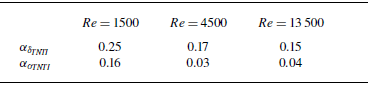
suggest the possible existence of a universal linear scaling in fully developed turbulent jets, i.e. for sufficiently large Reynolds numbers. We compute the slope of the thickness of the turbulent region
 $\alpha _{\delta _{\textit{TNTI}}}$
and of
 $\sigma _{\textit{TNTI}}$
within the fully developed turbulent region, and their values are reported in table 3 for Reynolds numbers larger than
 $Re\geqslant 1500$
. The growth rate of the turbulent regions settles at approximately
 $\alpha _{\textit{TNTI}}\approx 0.15$
, whereas the growth rate of the TNTI layer thickness settles at approximately
 $\alpha _\sigma \approx 0.04$
.
Slopes of the turbulent region thickness
 $\alpha _{\delta _{\textit{TNTI}}}$
and of the TNTI layer thickness
 $\alpha _{\sigma _{\textit{TNTI}}}$
.

 $(a)$
Box counting for the considered values of the Reynolds number; the number of boxes
 $N(r/h)$
is averaged in time, in the spanwise direction and in the streamwise direction (
 $Re=4500$
,
 $y/h\in [30;75]$
;
 $Re=13\,500$
,
 $y/h\in [30;65]$
).
 $(b)$
Fractal dimension of the interface computed via linear regression from the box counting. A semitransparent line is used to report the fractal dimension over the whole
 $h/r$
domain, whereas a solid line highlights the fractal dimension within the thickness of the TNTI layer (lower bound) and the Taylor length scale (upper bound). A black dashed line shows the analytic value
 $D_f=7/3$
(Sreenivasan et al. Reference Sreenivasan, Ramshankar and Meneveau1989; Sreenivasan Reference Sreenivasan1991).

We now aim at further characterising the TNTI: figure 15 shows that the shape of the TNTI is highly convoluted and characterised by smaller and smaller features for increasing Reynolds numbers and figure 16 showed that the TNTI layer has a finite thickness. These observations hints that the TNTI may have fractal dimension, as initially speculated by Mandelbrot (Reference Mandelbrot1974, Reference Mandelbrot1975) and later confirmed by Sreenivasan & Meneveau (Reference Sreenivasan and Meneveau1986). Fractals exhibit self-similarity over all scales; in a similar fashion, turbulence exhibits as well self-similarity although within a finite range of scale, bound between the problem scale and the Kolmogorov scale. We compute the fractal dimension of the TNTI in order to characterise the complexity of its shape, with a fractal dimension expected to be in the range
 $2 \leqslant D_f \leqslant 3$
: the dimension cannot be larger than the dimension of the space itself (three in our case) and with two being the minimum, since the TNTI is a surface in a three-dimensional space. The fractal dimension can be understood as how space-filling the TNTI is, or as a measure of the roughness of the TNTI (Sreenivasan & Meneveau Reference Sreenivasan and Meneveau1986). We extrapolate the fractal dimension
 $D_f$
using the box-counting method (Mandelbrot Reference Mandelbrot1982): for every size
 $r/h$
, we find the number of boxes
 $N(r/h)$
of size
 $r/h$
required to completely cover the TNTI, and then the fractal dimension can be computed as
 $D_f=\log (N(r/h))/\log (h/r)$
. The box-counting procedure is carried out on the three-dimensional TNTI; the number of boxes
 $N(r/h)$
is then averaged in time and in the turbulent region, i.e. in the entire spanwise direction and in the streamwise range where the PDF of the normalised enstrophy
 $\omega ^2/\hat {\omega }^2$
loses dependency on the streamwise coordinate. This region is identified as
 $y/h\in [30;75]$
for
 $Re=4500$
and
 $y/h\in [30;65]$
for
 $Re=13\,500$
. We show the box counting in figure 17
 $(a)$
for for
 $Re\geqslant 4500$
; we do not include here the two lowest Reynolds number cases, as they lack fully developed turbulence. The data from the box counting clearly hints at the existence of a linear growth in the logarithm of the number of boxes with the logarithm of the inverse of the box size within an intermediate range of scales, leading to the conclusion that the fractal dimension does not to depend on the box size
 $r/h$
. The local slope of
 $\log (N(r/h))$
, which corresponds to the fractal dimension
 $D_f$
, is computed via linear regression over 30 consecutive box-counting data points, and is shown in figure 17
 $(b)$
. A semitransparent line shows the fractal dimension over all scales, whereas the solid line identifies an intermediate regime bound between the Taylor length scale
 $\lambda$
(upper bound) and the thickness of the TNTI layer (lower bound). The Taylor length scale (sampled at the centreline in the turbulent region) is
 $\lambda \approx 0.09h$
for
 $Re=4500$
and
 $0.04h$
for
 $Re=13\,500$
. Within the intermediate range
 $[1/\sigma _{\textit{TNTI}},1/\lambda ]$
the fractal dimension is almost constant and equal to around
 $D_f\approx 2.4$
, while it reduces and approaches
 $D_f \to 2$
for decreasing length scales, indicating the absence of features of the TNTI at very small scales. The value obtained is slightly larger than that reported by Er et al. (Reference Er, Laval and Vassilicos2023) for a temporally evolving jet at
 $Re=3200$
, where the fractal dimension was reported to be in the range
 $2.09 \leqslant D_f \leqslant 2.18$
; we find instead very good agreement with the predicted value
 $D_f=7/3\approx 2.33$
for fully turbulent flows (Sreenivasan et al. Reference Sreenivasan, Ramshankar and Meneveau1989; Sreenivasan Reference Sreenivasan1991) and with previous experimental measurements with fractal dimension in the range
 $2.3\leqslant D_f\leqslant 2.4$
(Sreenivasan & Meneveau Reference Sreenivasan and Meneveau1986; Zubair & Catrakis Reference Zubair and Catrakis2009; Mistry et al. Reference Mistry, Philip, Dawson and Marusic2016, Reference Mistry, Dawson and Kerstein2018).
4. Conclusions
We investigated the dependence of the development of an incompressible planar jet on the Reynolds number via DNS. The Reynolds number, based on the inlet velocity and on the slit height, is changed between
 $500 \leqslant Re \leqslant 13\,500$
, being the widest range and largest values reached so far in DNS. This range of
 $Re$
spans the entire intermediate regime, where the flow shows a strong dependence on
 $Re$
: at
 $Re=500$
the flow is transitional and characterised by large-scale vortices, while at
 $Re=13\,500$
the flow is in a fully developed regime with an extended self-similar region. The aim of this work is to (i) corroborate existing experimental studies and provide a comprehensive characterisation of the Reynolds number effect on the flow, from near-inlet instabilities to the statistical properties in the turbulent self-similar region; (ii) determine, in the absence of any imposed inlet disturbances, the minimum Reynolds number above which a self-similar turbulent regime naturally emerges; and (iii) investigate detailed flow features at high Reynolds numbers, such as the TKE budget and the fractal properties of the three-dimensional TNTI, which remain difficult to access experimentally.
We found that the leading mode that destabilises the flow in the near-inlet region changes with
 $Re$
, confirming the results of previous experimental studies (see for example Deo et al. Reference Deo, Mi and Nathan2008). At low
 $Re$
(
 $Re\lt 1500$
), a sinusoidal mode dominates, resulting in a large-scale oscillation of the jet about the centreplane. At large
 $Re$
(
 $Re \geqslant 4500$
), a varicose mode dominates and the near-inlet flow retains the top/bottom symmetry. At intermediate
 $Re$
, instead, both modes are active. Our results show that, in agreement with their symmetries, the characteristic frequency of the sinusoidal mode is approximately half of that of the varicose mode.
We observe a clear dependence of the spreading rate of the jet on
 $Re$
, corroborating the experimental results of Namer & Ötügen (Reference Namer and Ötügen1988), Deo et al. (Reference Deo, Mi and Nathan2008) and Suresh et al. (Reference Suresh, Srinivasan, Sundararajan and Das2008). Our data show that as
 $Re$
increases, the spreading rate of the jet decreases up to
 $Re=4500$
, beyond which it becomes
 $Re$
-independent. This is due to the different relevance of the large-scale vortices, which are substantially absent in the large-
 $Re$
cases. A similar result is found for the centreline velocity (Namer & Ötügen Reference Namer and Ötügen1988; Deo et al. Reference Deo, Mi and Nathan2008; Suresh et al. Reference Suresh, Srinivasan, Sundararajan and Das2008): its decay is faster in low-
 $Re$
cases and becomes independent of
 $Re$
for
 $Re \geqslant 4500$
. Despite the faster decay rate of the centreline velocity for increasing
 $Re$
, the length of the potential core has an opposite trend. The potential core region shrinks as
 $Re$
increases, in agreement with the anticipated flow instabilities and transition to chaos/turbulent. The turbulence statistics show a clear dependence on
 $Re$
too. Our results show that the Reynolds stresses, the terms of the TKE budget and the energy spectra reach a self-similar regime for
 $Re \geqslant 4500$
only, where the flow statistics become independent of
 $Re$
. Although rather scattered, the self-similar Reynolds stresses profiles from our simulations at
 $Re=4500$
and
 $Re=13\,500$
are well within those reported in previous experimental and numerical studies at different
 $Re$
(Gutmark & Wygnanski Reference Gutmark and Wygnanski1976; Ramaprian & Chandrasekhara Reference Ramaprian and Chandrasekhara1985; Thomas & Prakash Reference Thomas and Prakash1991; Stanley et al. Reference Stanley, Sarkar and Mellado2002). The energy spectra start exhibiting signs of self-similarity for
 $Re \geqslant 1500$
. However, a well-developed inertial range of scales with the classical
 $\kappa _x^{-5/3}$
and
 $f^{-5/3}$
scaling, proxy of a fully turbulent regime, appears for
 $Re \geqslant 4500$
only.
We have then explored the effect of the Reynolds number on the TNTI, which separates the turbulent region (non-zero vorticity) from the non-turbulent region (irrotational flow). It is the first time that this is addressed in a systematic manner for a spatially evolving planar jet. An enstrophy-based criterion is used here to identify the TNTI; we discover that the normalisation proposed by Krug et al. (Reference Krug, Chung, Philip and Marusic2017) allows us to remove the dependency of the enstrophy threshold value on the Reynolds number and streamwise position. We identify a range of threshold values that allow to correctly define the TNTI, with values of the normalised enstrophy ranging from
 $10^{-6}$
up to
 $10^{-3}$
; the threshold value
 $10^{-5}$
has been selected in this work as it provides a clear separation of the turbulent and non-turbulent regions for all Reynolds numbers considered in this study. The thickness of the turbulent region identified by the TNTI shows a strong
 $Re$
dependence for the low-
 $Re$
cases (
 $Re \leqslant 1500$
), and converges towards a universal profile at large
 $Re$
(
 $Re\geqslant 4500$
). We report that the thickness of the turbulent region is approximately twice the jet thickness,
 $\delta _{\textit{TNTI}}/\delta _{0.5}\approx 2$
. Our results clearly show that as
 $Re$
increases,
 $\sigma _{\textit{TNTI}}$
reduces and the TNTI develops finer and finer structures. The small-scale shape of the TNTI is determined by the fine turbulence scales. It has been proven in the past (Mandelbrot Reference Mandelbrot1974, Reference Mandelbrot1975, Reference Mandelbrot1982; Sreenivasan & Meneveau Reference Sreenivasan and Meneveau1986) that turbulence has fractal properties within an intermediate range of scale. These properties apply as well to the TNTI: the boundary between the turbulent and non-turbulent regions thus has a non-integer (fractal) dimension,
 $2\leqslant D_f \leqslant 3$
. We find that the fractal dimension converges to
 $2.3\leqslant D_f \leqslant 2.35$
at large
 $Re$
, in perfect agreement with the theory developed by Sreenivasan et al. (Reference Sreenivasan, Ramshankar and Meneveau1989), Sreenivasan (Reference Sreenivasan1991) and with previous experimental measurements (Sreenivasan & Meneveau Reference Sreenivasan and Meneveau1986; Zubair & Catrakis Reference Zubair and Catrakis2009; Mistry et al. Reference Mistry, Philip, Dawson and Marusic2016, Reference Mistry, Dawson and Kerstein2018).
Acknowledgements
The authors acknowledge the computer time provided by the Scientific Computing & Data Analysis section of the Core Facilities at the Okinawa Institute of Science and Technology Graduate University (OIST), and the computational resources on SQUID provided by the HPCI System Research Project hp230018.
Funding
The research was supported by OIST with subsidy funding to M.E.R. from the Cabinet Office, Government of Japan.
Declaration of interests
The authors report no conflict of interest.
Appendix A. Grid independence test
To verify that the results are independent of the grid resolution, we have performed an additional simulation on a coarser grid for each value of the Reynolds number, with the coarse grid having approximately
 $N_c=0.75N$
, with
 $N_c$
and
 $N$
being the number of grid points in the streamwise and jet-normal directions for the coarse and standard grid, respectively. The total grid size for the coarse grid is thus
 $N_c/4\times N_c \times N_c$
, whereas for the standard grid is
 $N/4\times N \times N$
. Table 4 summarises the number of grid points for all cases, and the respective marker used in figure 18, where we show the centreline velocity
 $V_c$
and the jet thickness
 $\delta _{0.5}$
at both grid resolutions. A good agreement is observed for the data from the two kinds of grids, indicating that the chosen resolution in the standard grid is adequate to capture the dynamics of the jet. Note that, the deviations observed in the low-
 $Re$
cases are owed to the large vortical structures found towards the outlet, which would require much longer averaging times for the coarse grid case.
Summary of the grid resolution test cases;
 $N$
is the number of grid points used in the main simulations and
 $N_c$
is the number of grid points used in the coarse-grid simulations. The total number of grid points is also reported.

Grid independence tests for different Reynolds numbers, evaluated in terms of the
 $(a)$
centreline velocity and
 $(b)$
jet thickness.

The adequacy of the grid resolution is further demonstrated in figure 19, which shows the ratio of the local Kolmogorov scale to the grid spacing,
 $\eta _k/\varDelta$
, for
 $Re = 4500$
and
 $Re = 13\,500$
. The figure confirms that
 $\eta _k/\varDelta \gtrapprox 0.4$
in the region of interest, indicating that the smallest turbulent scales are resolved. Slight deviations near the inlet are expected, as the flow is not yet fully turbulent and the Kolmogorov scale is less well-defined in that region.
Size of the Kolmogorov length scale
 $\eta _k$
with respect to the grid resolution
 $\varDelta$
for the cases at high Reynolds number,
 $Re=4500$
in panel
 $(a)$
, and
 $Re=13\,500$
in panel
 $(b)$
.