1 Introduction
The length of the diffusive process is an important consideration in the study of phenomena modelled by diffusion. For example, consider the classical heat or diffusion equation
 $$ \begin{align} \frac{\partial u}{\partial t} = D \frac{\partial^2 u}{\partial x^2}, \quad 0 < x < L, \quad t> 0, \end{align} $$
where D is the diffusivity, L is the size of the one-dimensional domain and
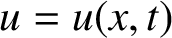 $u = u(x,t)$
describes the temperature or chemical concentration at position x and time t. Some reasonable initial and boundary conditions are usually added to equation (1.1) to complete the problem specification.
There are various ways to define the critical time. One common definition of the critical time [Reference Hickson, Barry, Sidhu and Mercer5] is the value
 $t^*$
, such that the average temperature distribution is a proportion of the average limiting temperature distribution (if it exists), that is,
 $$ \begin{align*}\frac{1}{L} \int_0^L u(x,t^*) \, dx = \frac{p}{L} \int_0^L u_\infty(x) \, dx, \quad 0 < p < 1. \end{align*} $$
An important application where the critical time is of practical interest is in steel annealing [Reference Barry and Sweatman1, Reference McGuinness, Sweatman, Baowan, Barry, Marchant and Edwards9], where a steel coil is heated by introducing an external temperature. The problem is to determine when (that is, the critical time) the coldest point in the coil reaches a given temperature. Other examples arise in the effectiveness of drug carriers [Reference Pontrelli and De Monte11] and the performance of electrodes [Reference Freger4]. Hickson et al. [Reference Hickson, Barry, Sidhu and Mercer5] investigated several definitions of the critical time for one- and two-layered diffusion problems, and the issue was briefly touched upon by Rodrigo and Worthy [Reference Rodrigo and Worthy15] for multi-layered diffusion. In all of these results, since the initial-boundary value problems (IBVPs) are linear, it is possible to solve these explicitly and the solution can be substituted into an appropriate critical time definition, thus yielding an equation for the critical time
 $t^*$
.
In a subsequent paper, Hickson et al. [Reference Hickson, Barry and Sidhu6] proposed three definitions of the critical time for a reaction–diffusion (RD) equation known as Fisher’s equation or the Fisher–KPP equation (named after Kolmogorov et al. [Reference Kolmogorov, Petrovsky and Piskunov8]), originally proposed as a model for the spread of an advantageous gene [Reference Fisher3]:
 $$ \begin{align} \frac{\partial u}{\partial t} = D \frac{\partial^2 u}{\partial x^2} + r u\, \bigg(1 - \frac{u}{K}\bigg), \quad 0 < x < L, \quad t> 0, \end{align} $$
where D is the diffusivity as before, L is the size of the one-dimensional habitat, r is the intrinsic growth rate, K is the carrying capacity and
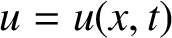 $u = u(x,t)$
is the population size or density at position x and at time t. In the absence of diffusion, the Fisher–KPP equation converts to the well-known logistic model. In nonbiological contexts, K is the solubility in mass transfer or the heat capacity in heat transfer. Hickson et al. [Reference Hickson, Barry and Sidhu6] studied the limiting case when
 $u \ll K$
, so that (1.2) again reduces to the linear equation
 $$ \begin{align*}\frac{\partial u}{\partial t} = D \frac{\partial^2 u}{\partial x^2} + r u, \quad 0 < x < L, \quad t> 0, \end{align*} $$
which can be solved analytically through a standard transformation to the heat equation. Hence substituting the explicit solution into each of the three critical time definitions allows one to estimate
 $t^*$
.
The main objective in this paper is to estimate the critical times for a general class of nonlinear RD equations defined on higher-dimensional domains. Let
 $\Omega \subset \mathbb R^n$
be a bounded domain with a sufficiently smooth boundary
 $\partial \Omega $
. Suppose that
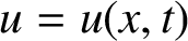 $u = u(x,t)$
satisfies the general Fisher–KPP equation
 $$ \begin{align} \frac{\partial u}{\partial t} = D \Delta u + f(u) \quad \text{in}\ \Omega \times (0,\infty). \end{align} $$
Note that the seminal work [Reference Kolmogorov, Petrovsky and Piskunov8] focused mainly on travelling wave solutions, which are considered over the unbounded domain
 $\Omega = \mathbb R$
. The general Fisher–KPP equation has been studied extensively (see, for instance, the exhaustive references in [Reference Britton2, Reference Murray10]). We assume that
 $f \in C^1([a,b])$
with
 $0 \le a < b$
, and
 $$ \begin{align*}f(a) = f(b) = 0, \quad f(y)> 0\quad \text{for all}\ a < y < b. \end{align*} $$
This means that
 $u_\infty = a$
(respectively,
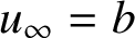 $u_\infty = b$
) is an unstable (respectively, stable) steady state of the associated kinetic system to (1.3). When
 $(a,b) = (0,K)$
and
 $f(y) = r y (1 - y/K)$
, the Fisher–KPP equation (1.2) is recovered from (1.3).
The initial condition is
 $$ \begin{align} u = u_0 \quad \text{in}\ \Omega, \end{align} $$
where
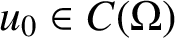 $u_0 \in C(\Omega )$
, say, and
 $a < u_0(x) < b$
for all
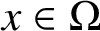 $x \in \Omega $
. We consider two types of boundary conditions (BCs). The first is a Dirichlet BC
 $$ \begin{align} u = h \quad \text{on}\ \partial \Omega \times (0,\infty), \end{align} $$
where
 $a < h(x) < b$
for all
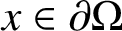 $x \in \partial \Omega $
, while the second is a no-flux or homogeneous Neumann BC,
 $$ \begin{align} \nabla u \cdot n = 0 \quad \text{on}\ \partial \Omega \times (0,\infty), \end{align} $$
where
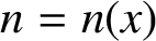 $n = n(x)$
is the outward normal vector at position x. For notational convenience and with a slight abuse of notation, we denote both BCs (1.5) and (1.6) by
 $$ \begin{align} B(u) = h \quad \text{on}\ \partial \Omega \times (0,\infty), \end{align} $$
with
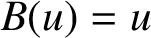 $B(u) = u$
,
 $h = h$
for the Dirichlet case and
 $B(u) = \nabla u \cdot n$
,
 $h = 0$
for the homogeneous Neumann case. In the context of population dynamics, the Dirichlet condition assumes that the species distribution is specified at the boundary, while the homogeneous Neumann condition assumes that no member of the species enters or leaves the domain. Therefore we study the IBVP (1.3)–(1.7).
Next, we introduce three definitions for the critical time that generalize those given in [Reference Hickson, Barry and Sidhu6]. Note that Hickson et al. [Reference Hickson, Barry and Sidhu6] considered a mixed BC in one dimension, while here Dirichlet and homogeneous Neumann BCs in arbitrary dimensions are considered.
-
(C1) The first definition of the critical time is that value of
 $t^*$
such that the average value of u is a proportion p of the average value of the asymptotic limit of u, that is, (1.8)where
$$ \begin{align} \frac{1}{m(\Omega)} \int_\Omega u(x,t^*) \, dx = \frac{p}{m(\Omega)} \int_\Omega u_\infty(x) \, dx, \quad 0 < p < 1, \end{align} $$
$m(\Omega )$
is the Lebesgue measure of
$\Omega $
and
$u_\infty = u_\infty (x)$
satisfies the steady-state problem Note that this definition has the drawback that one has to know the limiting distribution
$$ \begin{align*} & D \Delta u_\infty + f(u_\infty) = 0 \quad \text{in}\ \Omega, \\ & B(u_\infty) = h \quad \kern3pc\text{on}\ \partial \Omega. \end{align*} $$
$u_\infty $
, assuming it exists, to estimate the critical time. We keep
$m(\Omega )$
in (1.8) to emphasize that average values are being compared.
-
(C2) The second definition of the critical time is that value of
$t^*$
such that the average value of u is equal to a given value
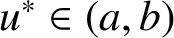
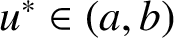
$u^* \in (a,b)$
, that is, (1.9)
$$ \begin{align} \frac{1}{m(\Omega)} \int_\Omega u(x,t^*) \, dx = u^*. \end{align} $$
-
(C3) Fix
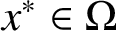
$x^* \in \Omega $
. The third definition of the critical time is that value of
$t^*$
such that the value of u at position
$x^*$
is equal to a given value
$u^* \in (a,b)$
, that is, (1.10)
$$ \begin{align} u(x^*,t^*) = u^*. \end{align} $$









Since (1.3)–(1.7) is a nonlinear problem, it is not possible to find the explicit solution in general, unlike the linear problems previously studied in the literature [Reference Hickson, Barry, Sidhu and Mercer5, Reference Hickson, Barry and Sidhu6]. Therefore, the idea we will pursue here is to find the bounding functions
 $u^-$
and
 $u^+$
such that
 $$ \begin{align*}u^-(x,t) \le u(x,t) \le u^+(x,t), \quad x \in \Omega, \quad t> 0, \end{align*} $$
and for which analytical expressions for
 $u^\pm $
can be obtained. Of course, we have to find
 $u^\pm $
that are “close” in some sense for all
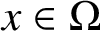 $x \in \Omega $
and
 $t> 0$
. If
 $t^*$
is taken as in any of the definitions (C1)–(C3) of the critical time given above, then we can derive upper and lower bounds for the critical time.
The outline of this paper is as follows. In Section 2, we determine a class of nonlinear RD equations that can be mapped to a linear diffusion equation, and then solve the associated IBVPs. These nonlinear, but linearizable, partial differential equations (PDEs) are used in Section 3 to construct upper and lower solutions for the general Fisher–KPP equation. Section 4 discusses how we can obtain bounds for the critical time with the aid of these comparison functions. In Section 5, we give an example using the one-dimensional Fisher–KPP equation and present the results of numerical simulations. Section 6 discusses some consequences of our result, in particular, how to estimate the critical time for a class of coupled RD equations that can be reduced to a scalar RD equation of Fisher–KPP type. We also discuss how we can extend the result of Section 2 to general RD systems. Section 7 gives a brief discussion and concludes the paper.
2 A linearizable nonlinear reaction–diffusion equation
Here, we look at transformations between classes of PDEs which will then be used to construct bounding functions for the solution to the general Fisher–KPP equation. We remark that the classes of PDEs considered in this section are slightly more general than the ones considered by Rodrigo [Reference Rodrigo12], and Rodrigo and Mimura [Reference Rodrigo and Mimura13], since the reaction terms are allowed to depend on t as well.
Define the operator
 $$ \begin{align*}N(t,u) = D \Delta u + f(t,u) - \frac{\partial u}{\partial t}, \end{align*} $$
where
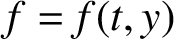 $f = f(t,y)$
is an arbitrary suitable function for the moment. Suppose that
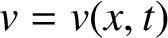 $v = v(x,t)$
satisfies the RD equation
 $$ \begin{align} \frac{\partial v}{\partial t} = D \Delta v + g(t,v) \end{align} $$
for some
 $C^1$
-function
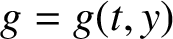 $g = g(t,y)$
. Let
 $u(x,t) = \Phi (t,v(x,t))$
, where
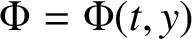 $\Phi = \Phi (t,y)$
is a
 $C^2$
-function that is strictly monotonic in y and satisfies the first-order PDE
 $$ \begin{align} \frac{\partial \Phi}{\partial t} + g(t,y) \frac{\partial \Phi}{\partial y} = f(t,\Phi). \end{align} $$
Note that
 $$ \begin{align} \Delta u = \frac{\partial \Phi}{\partial y}(t,v) \Delta v + \frac{\partial^2 \Phi}{\partial y^2}(t,v) \vert \nabla v \vert^2, \quad \vert \nabla u \vert^2 = \frac{\partial \Phi}{\partial y}(t,v)^2 \vert \nabla v \vert^2. \end{align} $$
Hence (2.3) gives
 $$ \begin{align*}N(t,u) = D \bigg[\frac{\partial \Phi}{\partial y}(t,v) \Delta v + \frac{\partial^2 \Phi}{\partial y^2}(t,v) \vert \nabla v \vert^2\bigg] + f(t,\Phi(t,v)) - \frac{\partial \Phi}{\partial t}(t,v) - \frac{\partial \Phi}{\partial y}(t,v) \frac{\partial v}{\partial t}. \end{align*} $$
 $$ \begin{align*} N(t,u) & = -g(t,v) \frac{\partial \Phi}{\partial y}(t,v) + D \frac{\partial^2 \Phi}{\partial y^2}(t,v) \vert \nabla v \vert^2 + f(t,\Phi(t,v)) - \frac{\partial \Phi}{\partial t}(t,v) \\ & = D \frac{\partial^2 \Phi}{\partial y^2}(t,v) \vert \nabla v \vert^2 \\ &= D \bigg[\bigg(\frac{\partial^2 \Phi}{\partial y^2}(t,v)\bigg)\,\bigg/\,\bigg(\frac{\partial \Phi}{\partial y}(t,v)^2\bigg)\bigg] \vert \nabla u \vert^2. \end{align*} $$
Therefore, u satisfies the PDE
 $$ \begin{align} \frac{\partial u}{\partial t} = D \Delta u + f(t,u) - D \bigg[\bigg(\frac{\partial^2 \Phi}{\partial y^2}(t,v)\bigg)\,\bigg/\,\bigg(\frac{\partial \Phi}{\partial y}(t,v)^2\bigg)\bigg] \vert \nabla u \vert^2 \end{align} $$
and solutions of the PDEs (2.1) and (2.4) are mapped to each other via the transformation
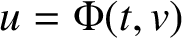 $u = \Phi (t,v)$
.
Remark 2.1 As a special case, when f, g and
 $\Phi $
are independent of t, (2.1) and (2.2) simplify to
 $$ \begin{align} \frac{\partial v}{\partial t} = D \Delta v + g(v) \end{align} $$
and
 $$ \begin{align} g(y) \Phi'(y) = f(\Phi(y)), \end{align} $$
respectively. Differentiating (2.6) with respect to y yields
 $$ \begin{align*}g(y) \Phi''(y) + g'(y) \Phi'(y) = f'(\Phi(y)) \Phi'(y), \end{align*} $$
so that
 $$ \begin{align*}\frac{\Phi''(y)}{\Phi'(y)^2} = \frac{f'(\Phi(y)) - g'(y)}{g(y) \Phi'(y)} = \frac{f'(\Phi(y)) - g'(y)}{f(\Phi(y))}. \end{align*} $$
Thus (2.4) becomes
 $$ \begin{align} \frac{\partial u}{\partial t} = D \Delta u + f(u) - D \frac{f'(u) - g'(v)}{f(u)} \vert \nabla u \vert^2, \end{align} $$
where v solves the RD equation (2.5) and
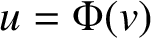 $u = \Phi (v)$
. If g is linear in y, say,
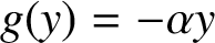 $g(y) = -\alpha y$
for some constant
 $\alpha \ne 0$
, then (2.5) reduces to the linear PDE
 $$ \begin{align} \frac{\partial v}{\partial t} = D \Delta v - \alpha v, \end{align} $$
while (2.7) simplifies to
 $$ \begin{align} \frac{\partial u}{\partial t} = D \Delta u + f(u) - D \frac{f'(u) + \alpha}{f(u)} \vert \nabla u \vert^2. \end{align} $$
This recovers the result in [Reference Rodrigo12, Reference Rodrigo and Mimura13] when f, g and
 $\Phi $
do not depend explicitly on t. Note that (2.9) is the general Fisher–KPP equation (1.3) but with an extra term. We will show later that the sign of this extra term can be controlled, which in turn will allow us to construct comparison functions for the solution of the general Fisher–KPP equation.
If we were to consider an associated Dirichlet problem, then solutions of the IBVPs
 $$ \begin{align*} & \frac{\partial u}{\partial t} = D \Delta u + f(t,u) - D\bigg[\bigg(\frac{\partial^2 \Phi}{\partial y^2}(t,v)\bigg)\,\bigg/\,\bigg(\frac{\partial \Phi}{\partial y}(t,v)^2\bigg)\bigg] \vert \nabla u \vert^2 \quad \text{in}\ \Omega \times (0,\infty),\\ & u = u_0 \quad \kern16.8pc\text{in}\ \Omega \times \{0\},\\ & u = h \quad \kern17.15pc\text{on}\ \partial \Omega \times (0,\infty), \end{align*} $$
and
 $$ \begin{align*} \begin{array}{ll} \dfrac{\partial v}{\partial t} = D \Delta v + g(t,v) &\quad \text{in}\ \Omega \times (0,\infty),\\ v = \Phi^{-1}(\cdot,u_0) &\quad \text{in}\ \Omega \times \{0\},\\ v = \Phi^{-1}(\cdot,h) &\quad \text{on}\ \partial \Omega \times (0,\infty) \end{array} \end{align*} $$
are mapped to each other via
 $u(x,t) = \Phi (t,v(x,t))$
, with
 $\Phi $
satisfying the first-order PDE (2.2). An analogous result holds for an associated homogeneous Neumann problem with IBVPs
 $$ \begin{align*} & \frac{\partial u}{\partial t} = D \Delta u + f(t,u) - D\bigg[\bigg(\frac{\partial^2 \Phi}{\partial y^2}(t,v)\bigg)\,\bigg/\,\bigg(\frac{\partial \Phi}{\partial y}(t,v)^2\bigg)\bigg] \vert \nabla u \vert^2 \quad \text{in}\ \Omega \times (0,\infty),\\ & u = u_0 \quad \kern16.75pc\text{in}\ \Omega \times \{0\},\\ & \nabla u \cdot n = 0 \quad \kern15.5pc\text{on}\ \partial \Omega \times (0,\infty) \end{align*} $$
and
 $$ \begin{align*} \begin{array}{ll} \dfrac{\partial v}{\partial t} = D \Delta v + g(t,v) &\quad \text{in}\ \Omega \times (0,\infty),\\ v = \Phi^{-1}(\cdot,u_0) &\quad \text{in}\ \Omega \times \{0\},\\ \nabla v \cdot n = 0 &\quad \text{on}\ \partial \Omega \times (0,\infty). \end{array} \end{align*} $$
In what follows we will be working with (2.8) and (2.9) as the linearity of (2.8) allows us to do some explicit computations. We will use these equations to solve the above associated IBVPs.
2.1 Solution of an associated Dirichlet problem
Here, we consider the Dirichlet problem
 $$ \begin{align} \begin{array}{ll} \displaystyle \frac{\partial u}{\partial t} = D \Delta u + f(u) - D \frac{f'(u) + \alpha}{f(u)} \vert \nabla u \vert^2 & \quad \text{in}\ \Omega \times (0,\infty), \\ \displaystyle u = u_0 &\quad \text{in}\ \Omega \times \{0\}, \\ \displaystyle u = h &\quad \text{on}\ \partial \Omega \times (0,\infty). \end{array} \end{align} $$
We state the following hypotheses. Firstly, we assume that for the linear eigenvalue problem
 $$ \begin{align*} \begin{array}{ll} \Delta \varphi + \lambda \varphi = 0& \quad \text{in}\ \Omega, \\ \varphi = 0 &\quad \text{on}\ \partial \Omega, \end{array} \end{align*} $$
the eigenvalues satisfy
 $0 < \lambda _1 < \lambda _2 \le \lambda _3 \le \cdots $
, so that
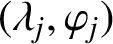 $(\lambda _j,\varphi _j)$
is an eigenpair for each
 $j = 1,2,\ldots .$
Moreover, we assume that there exists a positive solution
 $v_\infty = v_\infty (x)$
of the steady-state problem
 $$ \begin{align*} \begin{array}{ll} D \Delta v_\infty - \alpha v_\infty = 0 &\quad \text{in}\ \Omega, \\ v_\infty = \Phi^{-1}(h) &\quad \text{on}\ \partial \Omega. \end{array} \end{align*} $$
We can then transform (2.10) into
 $$ \begin{align*} \begin{array}{ll} \displaystyle \frac{\partial v}{\partial t} = D \Delta v - \alpha v &\quad \text{in}\ \Omega \times (0,\infty), \\ \displaystyle v = \Phi^{-1}(u_0) &\quad \text{in}\ \Omega \times \{0\}, \\ \displaystyle v = \Phi^{-1}(h) &\quad \text{on}\ \partial \Omega \times (0,\infty), \end{array} \end{align*} $$
where
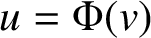 $u = \Phi (v)$
or
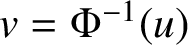 $v = \Phi ^{-1}(u)$
. Let
 $v(x,t) = v_\infty (x) + e^{-\alpha t} w(x,t)$
. Then w satisfies the homogeneous Dirichlet problem
 $$ \begin{align} \begin{array}{ll} \displaystyle \frac{\partial w}{\partial t} = D \Delta w &\quad \text{in}\ \Omega \times (0,\infty), \\ \displaystyle w = \Phi^{-1}(u_0) - v_\infty &\quad \text{in}\ \Omega \times \{0\}, \\ \displaystyle w = 0 &\quad \text{on}\ \partial \Omega \times (0,\infty). \end{array} \end{align} $$
Using a separation of variables technique, the formal solution of (2.11) is
 $$ \begin{align*}w(x,t) = \sum_{j = 1}^\infty c_j e^{-\lambda_j D t} \varphi_j(x), \quad c_j = \frac{\langle \Phi^{-1}(u_0) - v_\infty, \varphi_j \rangle}{\Vert \varphi_j \Vert^2}, \quad j = 1,2,\ldots, \end{align*} $$
where
 $\langle \cdot , \cdot \rangle $
and
 $\Vert \cdot \Vert $
denote the usual
 $L^2$
inner product and norm, respectively. Therefore the formal exact solution of the Dirichlet problem (2.10) is
 $$ \begin{align} u(x,t) = \Phi(v(x,t)), \quad v(x,t) = v_\infty(x) + \sum_{j = 1}^\infty c_j e^{-(\alpha + \lambda_j D) t} \varphi_j(x), \end{align} $$
where
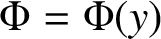 $\Phi = \Phi (y)$
solves the separable ordinary differential equation (ODE)
 $$ \begin{align} \alpha y \Phi'(y) + f(\Phi(y)) = 0 \end{align} $$
from (2.6).
2.2 Solution of an associated homogeneous Neumann problem
Next, we look at the homogeneous Neumann problem
 $$ \begin{align} \begin{array}{ll} \displaystyle \frac{\partial u}{\partial t} = D \Delta u + f(u) - D \frac{f'(u) + \alpha}{f(u)} \vert \nabla u \vert^2 &\quad \text{in}\ \Omega \times (0,\infty),\\ \displaystyle u = u_0 &\quad \text{in}\ \Omega \times \{0\}, \\ \displaystyle \nabla u \cdot n = 0 &\quad \text{on}\ \partial \Omega \times (0,\infty). \end{array} \end{align} $$
We make the following assumption. For the linear eigenvalue problem
 $$ \begin{align*} \begin{array}{ll} \Delta \varphi + \lambda \varphi = 0 &\quad \text{in}\ \Omega, \\ \nabla \varphi \cdot n = 0 &\quad \text{on}\ \partial \Omega, \end{array} \end{align*} $$
we assume that the eigenvalues satisfy
 $0 = \lambda _0 < \lambda _1 \le \lambda _2 \le \lambda _3 \le \cdots $
, so that
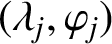 $(\lambda _j,\varphi _j)$
is an eigenpair for each
 $j = 0,1,\ldots .$
Note that
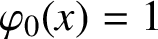 $\varphi _0(x) = 1$
may be taken without loss of generality.
Equations (2.8) and (2.9) transform (2.14) into
 $$ \begin{align*} \begin{array}{ll} \displaystyle \frac{\partial v}{\partial t} = D \Delta v - \alpha v &\quad \text{in}\ \Omega \times (0,\infty), \\ \displaystyle v = \Phi^{-1}(u_0) &\quad \text{in}\ \Omega \times \{0\}, \\ \displaystyle \nabla v \cdot n = 0 &\quad \text{on}\ \partial \Omega \times (0,\infty), \end{array} \end{align*} $$
with
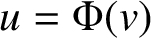 $u = \Phi (v)$
or
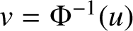 $v = \Phi ^{-1}(u)$
. Setting
 $v(x,t) = e^{-\alpha t} w(x,t)$
, we can easily see that
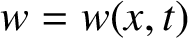 $w = w(x,t)$
satisfies the homogeneous Neumann problem
 $$ \begin{align} \begin{array}{ll} \displaystyle \frac{\partial w}{\partial t} = D \Delta w &\quad \text{in}\ \Omega \times (0,\infty), \\ \displaystyle w = \Phi^{-1}(u_0) &\quad \text{in}\ \Omega \times \{0\}, \\ \nabla w \cdot n = 0 &\quad \text{on}\ \partial \Omega \times (0,\infty). \end{array} \end{align} $$
Using a separation of variables technique, the formal solution of (2.15) is
 $$ \begin{align*} w(x,t) & = \frac{1}{m(\Omega)} \int_\Omega \Phi^{-1}(u_0(x)) \, dx + \sum_{j = 1}^\infty c_j e^{-\lambda_j D t} \varphi_j(x), \\ c_j & = \frac{\langle \Phi^{-1}(u_0), \varphi_j \rangle}{\Vert \varphi_j \Vert^2}, \quad j = 1,2,\ldots. \end{align*} $$
Note that we used Green’s identity here to deduce that
 $$ \begin{align*}\int_\Omega \varphi_j(x) \, dx = \langle \varphi_j, \varphi_0 \rangle = 0, \quad j = 1,2,\ldots. \end{align*} $$
Therefore the formal solution of the homogeneous Neumann problem (2.14) is
 $$ \begin{align} \begin{array}{ll} \displaystyle u(x,t) = \Phi(v(x,t)), \\ \displaystyle v(x,t) = e^{-\alpha t} \bigg[\frac{1}{m(\Omega)} \int_\Omega \Phi^{-1}(u_0(x)) \, dx + \sum_{j = 1}^\infty c_j e^{-\lambda_j D t} \varphi_j(x)\bigg], \end{array} \end{align} $$
where
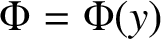 $\Phi = \Phi (y)$
again solves the separable ODE (2.13).
3 Upper and lower solutions for the general Fisher–KPP equation
Let
 $M = \sup _{a \le y \le b} \vert f'(y) \vert $
, and choose
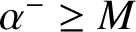 $\alpha ^- \ge M$
and
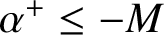 $\alpha ^+ \le - M$
. Let
 $u^\pm = u^\pm (x,t)$
satisfy the respective PDEs
 $$ \begin{align} \frac{\partial u^\pm}{\partial t} = D \Delta u^\pm + f(u^\pm) - D \frac{f'(u^\pm) + \alpha^\pm}{f(u^\pm)} \vert \nabla u^\pm \vert^2. \end{align} $$
Then
 $f'(u^-) + \alpha ^- \ge 0$
and
 $N(u^-) \ge 0$
if
 $a < u^- < b$
. Similarly,
 $f'(u^+) + \alpha ^+ \le 0$
and
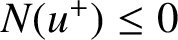 $N(u^+) \le 0$
if
 $a < u^+ < b$
. Assuming that
 $u^\pm $
satisfy the same initial and boundary conditions as u (that is,
 $u^\pm $
satisfy either (2.10) in the Dirichlet case or (2.14) in the homogeneous Neumann case), we deduce that
 $u^-$
is a lower solution and
 $u^+$
is an upper solution. Thus the solution u of the IBVP (1.3)–(1.7) for the general Fisher–KPP equation (1.3) satisfies
 $$ \begin{align} u^-(x,t) \le u(x,t) \le u^+(x,t), \quad x \in \Omega \cup \partial \Omega, \quad t \ge 0. \end{align} $$
Our task is to find
 $u^\pm $
. Let
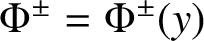 $\Phi ^\pm = \Phi ^\pm (y)$
be strictly monotonic
 $C^2$
-functions that satisfy the separable ODEs
 $$ \begin{align*}\alpha^\pm y \frac{d \Phi^\pm}{dy} + f(\Phi^\pm) = 0, \end{align*} $$
respectively. Suppose that
 $v^\pm = v^\pm (x,t)$
solve the respective linear PDEs
 $$ \begin{align*} \frac{\partial v^\pm}{\partial t} = \Delta v^\pm - \alpha^\pm v^\pm. \end{align*} $$
Then
 $u^\pm = \Phi ^\pm (v^\pm )$
; hence (3.2) is equivalent to
 $$ \begin{align*} \Phi^-(v^-(x,t)) \le u(x,t) \le \Phi^+(v^+(x,t)), \quad x \in \Omega \cup \partial \Omega, \quad t \ge 0. \end{align*} $$
Once
 $v^\pm $
have been determined, then
 $u^\pm $
will be known and therefore (3.2) will hold. In the next two subsections, we will find the bounding functions
 $u^\pm $
.
3.1 Bounding functions for the Dirichlet problem
To (3.1) we add initial and Dirichlet BCs, namely,
 $$ \begin{align*} \begin{array}{ll} \dfrac{\partial u^\pm}{\partial t} = D \Delta u^\pm + f(u^\pm) - D \dfrac{f'(u^\pm) + \alpha^\pm}{f(u^\pm)} \vert \nabla u^\pm \vert^2 & \quad \text{in}\ \Omega \times (0,\infty), \\ u^\pm = u_0 &\quad \text{in}\ \Omega \times \{0\}, \\ u^\pm = h &\quad \text{on}\ \partial \Omega \times (0,\infty). \end{array} \end{align*} $$
Using (2.12), we obtain the bounding functions
 $$ \begin{align*} \begin{split} u^\pm(x,t) & = \Phi^\pm(v^\pm(x,t)),\\ v^\pm(x,t) & = v_\infty^\pm(x) + \sum_{j = 1}^\infty c_j^\pm e^{-(\alpha^\pm + \lambda_j D) t} \varphi_j(x), \end{split} \end{align*} $$
where
 $$ \begin{align*}c_j^\pm = \frac{\langle (\Phi^\pm)^{-1}(u_0) - v_\infty^\pm, \varphi_j \rangle}{\Vert \varphi_j \Vert^2}, \quad j = 1,2,\ldots, \end{align*} $$
and
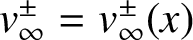 $v_\infty ^\pm = v_\infty ^\pm (x)$
solve the respective problems
 $$ \begin{align*} \begin{array}{ll} D \Delta v_\infty^\pm - \alpha^\pm v_\infty^\pm = 0 &\quad \text{in}\ \Omega, \\ v_\infty^\pm = (\Phi^\pm)^{-1}(h) &\quad \text{on}\ \partial \Omega. \end{array} \end{align*} $$
As mentioned previously, these bounding functions satisfy (3.2).
Remark 3.1 Let us take a look at some consequences for
 $v^\pm $
when
 $t \rightarrow \infty $
, for each x. We see that
 $\alpha ^- + \lambda _1 D \ge M + \lambda _1 D> 0$
, which implies that
 $v^-(x,t) \rightarrow v_\infty ^-(x)$
as
 $t \rightarrow \infty $
. Moreover, there are three possibilities for the limit of
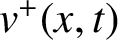 $v^+(x,t)$
.
-
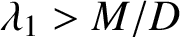
(i) Suppose that
$\lambda _1>M/D$
. If
$-\lambda _1 D < \alpha ^+ \le -M$
, then and therefore
$$ \begin{align*}0 < \alpha^+ + \lambda_1 D < \alpha^+ + \lambda_2 D \le \alpha^+ + \lambda_3 D \le \cdots ,\end{align*} $$
$v^+(x,t) \rightarrow v_\infty ^+(x)$
as
$t \rightarrow \infty $
. If
$\alpha ^+ = -\lambda _1 D$
, then as
$$ \begin{align*}0 = \alpha^+ + \lambda_1 D < \alpha^+ + \lambda_2 D \le \alpha^+ + \lambda_3 D \le\cdots \ \ \, \text{and} \ \ \, v^+(x,t) \rightarrow v_\infty^+(x) + c_1^+ \varphi_1(x)\end{align*} $$
$t \rightarrow \infty $
. Finally, if
$\alpha ^+ < -\lambda _1 D$
, then
$v^+(x,t) \rightarrow \infty $
as
$t \rightarrow \infty $
.
-
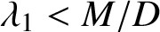
(ii) Suppose that
$\lambda _1 <M/D$
. Since
$\alpha ^+ \le -M < -\lambda _1 D$
, we deduce that
$v^+(x,t) \rightarrow \infty $
as
$t \rightarrow \infty $
. -
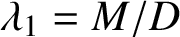
(iii) Suppose that
$\lambda _1 =M/D$
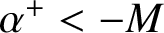
. If
$\alpha ^+ < -M$
, then
$\alpha ^+ < -\lambda _1 D$
and
$v^+(x,t) \rightarrow \infty $
as
$t \rightarrow ~\infty $
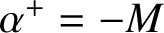
. On the other hand, if
$\alpha ^+ = -M$
, then Thus
$$ \begin{align*}0 = \alpha^+ + \lambda_1 D < \alpha^+ + \lambda_2 D \le \alpha^+ + \lambda_3 \le \cdots .\end{align*} $$
$v^+(x,t) \rightarrow v_\infty ^+(x) + c_1^+ \varphi _1(x)$
as
$t \rightarrow \infty $
.



















3.2 Bounding functions for the homogeneous Neumann problem
Consider (3.1) with initial and homogeneous Neumann BCs, that is,
 $$ \begin{align*} & \frac{\partial u^\pm}{\partial t} = D \Delta u^\pm + f(u^\pm) - D \frac{f'(u^\pm) + \alpha^\pm}{f(u^\pm)} \vert \nabla u^\pm \vert^2 \quad \text{in}\ \Omega \times (0,\infty),\\ & u^\pm = u_0 \quad \kern12.6pc\text{in}\ \Omega \times \{0\}, \\ & \nabla u^\pm \cdot n = 0 \quad \kern11.31pc\text{on}\ \partial \Omega \times (0,\infty). \end{align*} $$
Using (2.16), we obtain
 $$ \begin{align*} u^\pm(x,t) & = \Phi^\pm(v^\pm(x,t)),\\ v^\pm(x,t) & = e^{-\alpha^\pm t} \bigg[\frac{1}{m(\Omega)} \int_\Omega (\Phi^\pm)^{-1}(u_0(x)) \, dx + \sum_{j = 1}^\infty c_j^\pm e^{-\lambda_j D t} \varphi_j(x)\bigg], \end{align*} $$
where
 $$ \begin{align*}c_j^\pm = \frac{\langle (\Phi^\pm)^{-1}(u_0), \varphi_j \rangle}{\Vert \varphi_j \Vert^2}, \quad j = 1,2,\ldots. \end{align*} $$
Remark 3.2 Fix x. As
 $\alpha ^- \ge M> 0$
, we have
 $v^-(x,t) \rightarrow 0$
as
 $t \rightarrow \infty $
. Similarly,
 $\alpha ^+ \le -M < 0$
, so that
 $v^+(x,t) \rightarrow \infty $
as
 $t \rightarrow \infty $
.
4 Bounds for the critical time
We now derive bounds for the critical time. For the first critical time definition (1.8), we have
 $$ \begin{align*} \frac{1}{m(\Omega)} \int_\Omega \Phi^-(v^-(x,t^*)) \, dx \le \frac{p}{m(\Omega)} \int_\Omega u_\infty(x) \, dx \le \frac{1}{m(\Omega)} \int_\Omega \Phi^+(v^+(x,t^*)) \, dx. \end{align*} $$
For the second critical time definition (1.9), we obtain
 $$ \begin{align} \frac{1}{m(\Omega)} \int_\Omega \Phi^-(v^-(x,t^*)) \, dx \le u^* \le \frac{1}{m(\Omega)} \int_\Omega \Phi^+(v^+(x,t^*)) \, dx. \end{align} $$
Finally, the third critical time definition (1.10) gives
 $$ \begin{align} \Phi^-(v^-(x^*,t^*)) \le u^* \le \Phi^+(v^+(x^*,t^*)). \end{align} $$
In the above expressions,
 $v^\pm $
and
 $\phi ^\pm $
are known in principle since they solve linear IBVPs and separable ODEs, respectively.
As an example to illustrate how to obtain bounds for the critical time, suppose that we consider (4.1). Define the functions
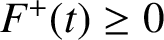
 $$ \begin{align*} F^-(t) & = u^* - \frac{1}{m(\Omega)} \int_\Omega \Phi^-(v^-(x,t)) \, dx, \\ F^+(t) & = \frac{1}{m(\Omega)} \int_\Omega \Phi^+(v^+(x,t)) \, dx - u^*. \end{align*} $$
Hence we want to determine all values of
 $t \ge 0$
for which
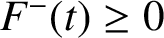 $F^-(t)\ge 0$
and
 $F^+(t) \ge 0$
, from which we obtain intervals for such values of t and therefore bounds for
 $t^*$
. In general, this has to be performed numerically. Analogous definitions for
 $F^\pm (t)$
can be given for the other critical time definitions.
5 Example: Fisher–KPP equation in one dimension
Consider the one-dimensional Fisher–KPP equation with
 $\Omega = (0,L)$
, where
 $L> 0$
. Take
 $(a,b) = (0,K)$
, where
 $K> 0$
is the carrying capacity, and
 $f(y) = r y (1 - y/K)$
. As
 $f'(y) = r (1 - 2 y/K)$
, we see that
 $M = \sup _{0 \le y \le K} \vert f'(y) \vert = r$
. Solving the separable ODE (2.13) yields
 $$ \begin{align*}\Phi(y) = \frac{c K y^{-r/\alpha}}{1 + y^{-r/\alpha}}, \end{align*} $$
where
 $c> 0$
is an arbitrary constant of integration. For simplicity we take
 $c = 1$
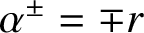
, although other choices are possible. Choose
 $\alpha ^\pm = \mp r$
, for instance, so that
 $$ \begin{align*} && \Phi^-(y) &= \frac{K}{1 + K y}, \qquad \Phi^+(y) = \frac{K y}{K + y}, \\ &&(\Phi^-)^{-1}(y)& = \frac{K - y}{K y}, \qquad (\Phi^+)^{-1}(y) = \frac{K y}{K - y}. \end{align*} $$
Thus
 $$ \begin{align} u^-(x,t) = \frac{K}{1 + K v^-(x,t)}, \quad u^+(x,t) = \frac{K v^+(x,t)}{K + v^+(x,t)}, \end{align} $$
where
 $v^\pm $
satisfy the respective linear PDEs
 $$ \begin{align*}\frac{\partial v^-}{\partial t} = D \frac{\partial^2 v^-}{\partial x^2} - r v^-, \quad \frac{\partial v^+}{\partial t} = D \frac{\partial^2 v^+}{\partial x^2} + r v^+. \end{align*} $$
The functions
 $u^\pm $
solve the nonlinear PDEs
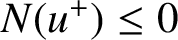
 $$ \begin{align*} \frac{\partial u^-}{\partial t} & = D \frac{\partial^2 u^-}{\partial x^2} + r u^- \bigg(1 - \frac{u^-}{K}\bigg) - \frac{2 D}{u^-} \bigg(\frac{\partial u^-}{\partial x}\bigg)^2, \\ \frac{\partial u^+}{\partial t} & = D \frac{\partial^2 u^+}{\partial x^2} + r u^+ \bigg(1 - \frac{u^+}{K}\bigg) + \frac{2 D}{K - u^+} \bigg(\frac{\partial u^+}{\partial x}\bigg)^2, \end{align*} $$
respectively. As expected,
 $N(u^-) \ge 0$
and
 $N(u^+) \le 0$
if
 $0 < u^\pm < K$
.
5.1 Dirichlet problem
In this case, the boundary conditions are
 $u(0,t) = h(0) \in (0,K)$
and
 $u(L,t) = h(L) \in (0,K)$
. The eigenpairs are
 $$ \begin{align*}\lambda_j = \bigg(\frac{j \pi}{L}\bigg)^2, \quad \varphi_j(x) = \sin\bigg(\frac{j \pi x}{L}\bigg), \quad j = 1,2,\ldots. \end{align*} $$
The solutions of the problems
 $$ \begin{align*} D (v^-_\infty)'' - r v^-_\infty &= 0 \quad \text{in}\ (0,L), \quad v^-_\infty(0) = \frac{K - h(0)}{K h(0)}, \quad v^-_\infty(L) = \frac{K - h(L)}{K h(L)}, \\[2mm] D (v^+_\infty)'' + r v^+_\infty &= 0 \quad \text{in}\ (0,L), \quad v^+_\infty(0) = \frac{K h(0)}{K - h(0)}, \quad v^+_\infty(L) = \frac{K h(L)}{K - h(L)} \end{align*} $$
are
 $$ \begin{align*} v^-_\infty(x) & = \operatorname{\mathrm{csch}}\bigg(\sqrt{\frac{r}{D}} L\bigg) \bigg[\frac{K - h(0)}{K h(0)} \sinh \bigg(\sqrt{\frac{r}{D}}(L - x)\bigg) + \frac{K - h(L)}{K h(L)} \sinh\bigg(\sqrt{\frac{r}{D}}x\bigg)\bigg], \\[2mm] v^+_\infty(x) & = \csc\bigg(\sqrt{\frac{r}{D}} L\bigg) \bigg[\frac{K h(0)}{K - h(0)} \sin\bigg(\sqrt{\frac{r}{D}}(L - x)\bigg) + \frac{K h(L)}{K - h(L)} \sin\bigg(\sqrt{\frac{r}{D}}x\bigg)\bigg], \end{align*} $$
respectively. Then
 $$ \begin{align} \begin{array}{l} \displaystyle v^-(x,t) = v^-_\infty(x) + \sum_{j = 1}^\infty c_j^- e^{-(r + ({j^2 \pi^2 D}/{L^2})) t} \sin\bigg(\frac{j \pi x}{L}\bigg),\\ \displaystyle c_j^- = \frac{2}{L} \int_0^L \bigg[\frac{K - u_0(x)}{K u_0(x)} - v^-_\infty(x)\bigg] \sin\bigg(\frac{j \pi x}{L}\bigg) \, dx, \quad j = 1,2,\ldots,\\ \displaystyle v^+(x,t) = v^+_\infty(x) + \sum_{j = 1}^\infty c_j^+ e^{(r - ({j^2 \pi^2 D}/{L^2})) t} \sin\bigg(\frac{j \pi x}{L}\bigg),\\ \displaystyle c_j^+ = \frac{2}{L} \int_0^L \bigg[\frac{K u_0(x)}{K - u_0(x)} - v^+_\infty(x)\bigg] \sin\bigg(\frac{j \pi x}{L}\bigg) \, dx, \quad j = 1,2,\ldots. \end{array} \end{align} $$
Thus the solution u of the Fisher–KPP equation for the Dirichlet problem is bounded by
 $$ \begin{align*}\frac{K}{1 + K v^-(x,t)} \le u(x,t) \le \frac{K v^+(x,t)}{K + v^+(x,t)}, \quad 0 \le x \le L, \quad t \ge 0, \end{align*} $$
where
 $v^\pm $
are given in (5.2).
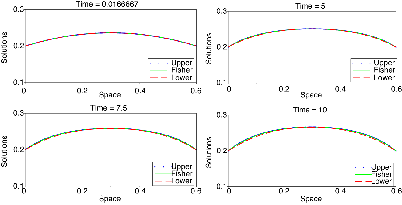
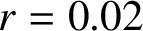
Next, we present the numerical results for the Dirichlet problem. Set
 $D = 0.0008$
,
 $r = 0.02$
,
 $K = 1$
,
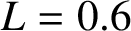 $L = 0.6$
and
 $T = 10$
. Choose
 $$ \begin{align*}u_0(x) = 0.4 x (L - x) + 0.2 K, \quad h(x) = 0.2 K \end{align*} $$
for the initial condition and boundary function, respectively. Profiles of the upper and lower solutions, as well as the solution of the Fisher–KPP equation, are shown in Figure 1 for different time values. To estimate the critical time, we follow the procedure outlined in Section 4. All numerical simulations were performed in Scilab.
Profiles of
 $u^\pm $
and u for the Dirichlet case when
 $t = 0.0166667, 5, 7.5, 10$
.

For the first critical time definition, suppose that
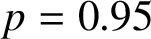 $p = 0.95$
. The actual critical time obtained by solving the Fisher–KPP equation numerically is
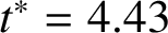 $t^* = 4.43$
. We obtain the bounds
 $4.38 \le t^* \le 4.7$
from the comparison functions (5.1), (5.2). For the second critical time definition, suppose that
 $u^* = 0.24 K$
. Then the actual critical time estimated by solving Fisher’s equation numerically is
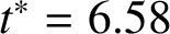 $t^* = 6.58$
, while the comparison functions (5.1), (5.2) yield the bounds
 $6.5 \le t^* \le 7.05$
. Finally, for the third critical time definition, take
 $x^* = 0.45$
and
 $u^* = 0.24 K$
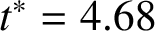
. The actual critical time calculated by solving Fisher’s equation numerically is
 $t^* = 4.68$
, whereas the bounds obtained from (5.1) and (5.2) are
 $4.65 \le t^* \le 4.95$
.
5.2 Homogeneous Neumann problem
In this case, the boundary conditions are
 $$ \begin{align*}\frac{\partial u}{\partial x}(0,t) = \frac{\partial u}{\partial x}(L,t) = 0,\end{align*} $$
and the eigenpairs are
 $$ \begin{align*}\lambda_j = \bigg(\frac{j \pi}{L}\bigg)^2, \quad \varphi_j(x) = \cos\bigg(\frac{j \pi x}{L}\bigg), \quad j = 0,1,\ldots. \end{align*} $$
Then
 $$ \begin{align} \begin{array}{l} \displaystyle v^-(x,t) = e^{-r t} \bigg[\frac{1}{L} \int_0^L \frac{K - u_0(x)}{K u_0(x)} \, dx + \sum_{j = 1}^\infty c_j^- e^{-({j^2 \pi^2 D})/({L^2}) t} \cos\bigg(\frac{j \pi x}{L}\bigg)\bigg],\\ \displaystyle c_j^- = \frac{2}{L} \int_0^L \frac{K - u_0(x)}{K u_0(x)} \cos\bigg(\frac{j \pi x}{L}\bigg) \, dx, \quad j = 1,2,\ldots,\\ \displaystyle v^+(x,t) = e^{r t} \bigg[\frac{1}{L} \int_0^L \frac{K u_0(x)}{K - u_0(x)} \, dx + \sum_{j = 1}^\infty c_j^+ e^{-({j^2 \pi^2 D})/({L^2}) t} \cos\bigg(\frac{j \pi x}{L}\bigg)\bigg],\\ \displaystyle c_j^+ = \frac{2}{L} \int_0^L \frac{K u_0(x)}{K - u_0(x)} \cos\bigg(\frac{j \pi x}{L}\bigg) \, dx, \quad j = 1,2,\ldots. \end{array} \end{align} $$
As in the Dirichlet case, the solution u of the Fisher–KPP equation is bounded by
 $$ \begin{align*}\frac{K}{1 + K v^-(x,t)} \le u(x,t) \le \frac{K v^+(x,t)}{K + v^+(x,t)}, \quad 0 \le x \le L, \quad t \ge 0, \end{align*} $$
where
 $v^\pm $
are given in (5.3).
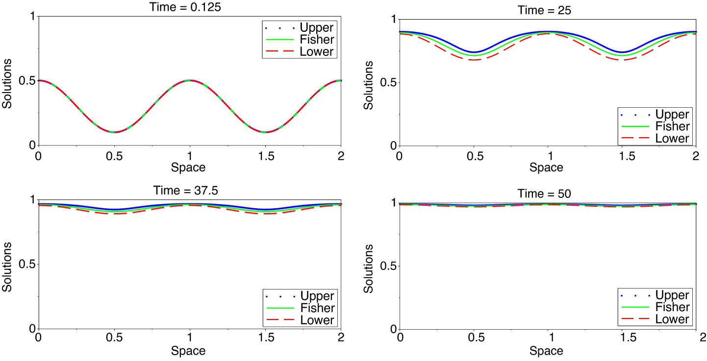
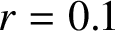
To present numerical results for the homogeneous Neumann problem, set
 $D = 0.0005$
,
 $r = 0.1$
,
 $K = 1$
,
 $L = 2$
and
 $T = 50$
. Choose
 $$ \begin{align*}u_0(x) = 0.2 \cos\bigg(\frac{4 \pi x}{L}\bigg) + 0.3 K \end{align*} $$
for the initial condition. Profiles of the upper and lower solutions, as well the solution of the Fisher–KPP equation, are shown in Figure 2 for different time values.
Profiles of
 $u^\pm $
and u for the homogeneous Neumann case when
 $t = 0.125, 25, 37.5, 50$
.

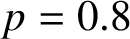
For the first critical time definition, suppose that
 $p = 0.8$
. The actual critical time obtained by solving the Fisher–KPP equation numerically is
 $t^* = 23.13$
. From (5.1), (5.3) we obtain the bounds
 $21.63 \le t^* \le 25$
. For the second critical time definition, suppose that
 $u^* = 0.8 K$
. Then the actual critical time estimated by solving the Fisher–KPP equation numerically is
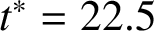 $t^* = 22.5$
, while the comparison functions (5.1), (5.3) yield the bounds
 $22.5\le t^* \le 25.87$
. Finally, for the third critical time definition, take
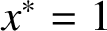 $x^* = 1$
and
 $u^* = 0.8 K$
. The actual critical time calculated by solving the Fisher–KPP equation numerically is
 $t^* = 16.13$
, whereas the bounds obtained from (5.1), (5.3) are
 $15.88 \le t^* \le 16.75$
.
6 Extensions to systems of reaction–diffusion equations
A natural question to ask is whether our approach to constructing comparison functions will work for systems of RD equations. In general, this is not possible unless there is also a comparison principle for such systems. Nevertheless, there are some classes of RD systems which permit the reduction to a scalar RD equation of Fisher–KPP type, for which the results in this paper can be applied.
For example, consider the following class of RD systems:
 $$ \begin{align} \begin{array}{l} \displaystyle \frac{\partial u}{\partial t} = v f(u),\\[12pt] \displaystyle \frac{\partial v}{\partial t} = D \Delta v + v g(u). \end{array} \end{align} $$
An example where this class of RD systems arises is in the spatial spread and control of rabies [Reference Källén, Arcuri and Murray7]. The quantities
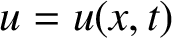 $u = u(x,t)$
and
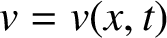 $v = v(x,t)$
are the susceptible and infective population densities of foxes, respectively, with
 $f(u) = - K u$
and
 $g(u) = K u - \mu $
. The parameter K is a transmission coefficient and
 $1/\mu $
is the life expectancy of an infective fox. In this case, it would be of interest to know the critical time when the average infective fox population density reaches a certain value.
We now show that (6.1) can be reduced to a scalar RD equation of the type considered previously. Define
 $$ \begin{align} w(x,t) = w_0(x) + \int_0^t v(x,\tau) \, d \tau, \end{align} $$
so that
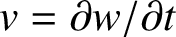 $v =\partial w/\partial t$
. Integrating the second equation in (6.1) from
 $\tau = 0$
to
 $\tau = t$
, we obtain
 $$ \begin{align*}v(x,t) - v_0(x) = D \Delta w(x,t) - D \Delta w_0(x) + \int_0^t g(u(x,\tau)) v(x,\tau) \, d\tau. \end{align*} $$
Substituting the first equation in (6.1) into the previous equation gives
 $$ \begin{align} v(x,t) - v_0(x) & = D \Delta w(x,t) - D \Delta w_0(x) + \int_0^t \frac{g(u(x,\tau))}{f(u(x,\tau))} \frac{\partial u}{\partial \tau}(x,\tau) \, d \tau \nonumber \\ \displaystyle & = D \Delta w(x,t) - D \Delta w_0(x) + \int_{u_0(x)}^{u(x,t)} \frac{g(z)}{f(z)} \, dz. \end{align} $$
Define
 $$ \begin{align*}F(y;y_0) = \int_{y_0}^y \frac{g(z)}{f(z)} \, dz, \quad G(y;y_0) = \int_{y_0}^y \frac{1}{f(z)} \, dz, \end{align*} $$
and suppose that G is invertible. We see from (6.3) that
 $$ \begin{align} \frac{\partial w}{\partial t} = D \Delta w + F(u;u_0) + v_0 - \Delta w_0. \end{align} $$
But (6.2) and the first equation in (6.1) yield
 $$ \begin{align*}w(x,t) = w_0(x) + \int_0^t \frac{1}{f(u(x,\tau))} \frac{\partial u}{\partial \tau}(x,\tau) \, d \tau = w_0(x) + \int_{u_0(x)}^{u(x,t)} \frac{1}{f(z)} \, dz, \end{align*} $$
that is,
 $w = w_0 + G(u;u_0)$
. Hence
 $u = G^{-1}(w - w_0;u_0)$
and (6.4) gives
 $$ \begin{align*}\frac{\partial w}{\partial t} = D \Delta w + F(G^{-1}(w - w_0;u_0);u_0) + v_0 - \Delta w_0. \end{align*} $$
Therefore, the RD system (6.1) is equivalent to the scalar RD equation
 $$ \begin{align*}\frac{\partial w}{\partial t} = D \Delta w + H(w;u_0,v_0,w_0), \end{align*} $$
where
 $$ \begin{align*}H(w;u_0,v_0,w_0) = F(G^{-1}(w - w_0;u_0);u_0) + v_0 - \Delta w_0. \end{align*} $$
In particular, if
 $u_0$
,
 $v_0$
and
 $w_0$
are constants, then H does not depend explicitly on x.
As an example, consider the (nondimensionalized) rabies model mentioned above [Reference Källén, Arcuri and Murray7]:
 $$ \begin{align} \begin{array}{l} \displaystyle \frac{\partial u}{\partial t} = -u v,\\[12pt] \displaystyle \frac{\partial v}{\partial t} = \Delta v + u v - r v. \end{array} \end{align} $$
Here,
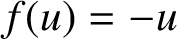 $f(u) = -u$
,
 $g(u) = u - r$
and
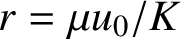 $r = \mu u_0/K$
is a measure of the mortality rate as compared with the contact rate. Then
 $$ \begin{align*}F(y;y_0) = -(y - y_0) + r \log\bigg(\frac{y}{y_0}\bigg), \quad G(y;y_0) = -\log\bigg(\frac{y}{y_0}\bigg), \quad G^{-1}(y;y_0) = y_0 e^{-y}. \end{align*} $$
Hence
 $$ \begin{align*}H(w;u_0,v_0,w_0) = u_0 [1 - e^{-(w - w_0)}] -r (w - w_0) + v_0 - \Delta w_0. \end{align*} $$
Suppose that
 $u_0$
,
 $v_0$
and
 $w_0$
are all constants. Then, suppressing the dependence on these parameters, we have
 $$ \begin{align*}H(w) = u_0 [1 - e^{-(w - w_0)}] - r (w - w_0) + v_0 \end{align*} $$
and we can instead study the RD equation
 $$ \begin{align} \frac{\partial w}{\partial t} = \Delta w + u_0 [1 - e^{-(w - w_0)}] - r (w - w_0) + v_0. \end{align} $$
Consider the curves
 $$ \begin{align*}\Gamma_1 : y \mapsto u_0 [1 - e^{-(y - w_0)}], \quad \Gamma_2 : y \mapsto r (y - w_0) - v_0 \end{align*} $$
such that
 $-r w_0 - v_0> u_0 (1 - e^{w_0})$
. Then there will be two points of intersection (say, a and b) of
 $\Gamma _1$
and
 $\Gamma _2$
such that
 $0 < a < w_0 < b$
and the graph of
 $\Gamma _1$
will always be above the graph of
 $\Gamma _2$
for all
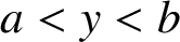 $a < y < b$
. This means that
 $H(a) = H(b) = 0$
and
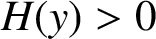 $H(y)> 0$
for all
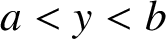 $a < y < b$
, that is, (6.6) is of Fisher–KPP type. The results previously obtained, pertaining to comparison functions and bounds for the critical times for the Fisher–KPP equation, can therefore be used to estimate the critical times for the RD system (6.5).
The procedure for constructing a linearizable nonlinear RD equation given in Section 2 can be generalized to systems of RD equations, provided the diffusion coefficients are all equal. Consider the following system of RD equations for
 $u_i = u_i(x,t)$
for all
 $i = 1,2,\ldots ,m$
:
 $$ \begin{align} \frac{\partial u_i}{\partial t} = D \Delta u_i + f_i(t,u_1,u_2,\ldots,u_m), \quad i = 1,2,\ldots,m. \end{align} $$
In matrix notation, this can be expressed as
 $\partial u/\partial t = D \Delta u + f(t,u)$
in the obvious way, where D is a positive scalar that may be scaled out. Following the idea for the scalar case, suppose that
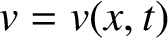 $v = v(x,t)$
satisfies the scalar PDE
 $$ \begin{align*}\frac{\partial v}{\partial t} = D \Delta v + g(t,v). \end{align*} $$
Let
 $u_i(x,t) = \Phi _i(t,v(x,t))$
for each
 $i = 1,2,\ldots ,m$
, where
 $\Phi _i = \Phi _i(t,y)$
for all
 $i = 1,2,\ldots ,m$
satisfy the system of first-order PDEs
 $$ \begin{align*}\frac{\partial \Phi_i}{\partial t} + g(t,y) \frac{\partial \Phi_i}{\partial y} = f_i(t,\Phi_1,\Phi_2,\ldots,\Phi_m), \quad i = 1,2,\ldots,m, \end{align*} $$
which are equivalent to the matrix system
 $$ \begin{align*}\frac{\partial \Phi}{\partial t} + g(t,y) \frac{\partial \Phi}{\partial y} = f(t,\Phi)\end{align*} $$
in the obvious way. We observe that
 $$ \begin{align*}\Delta u_i = \frac{\partial \Phi_i}{\partial y}(t,v) \Delta v + \frac{\partial^2 \Phi_i}{\partial y^2}(t,v) \vert \nabla v \vert^2, \quad \vert \nabla u_i \vert^2 = \frac{\partial \Phi_i}{\partial y}(t,v)^2 \vert \nabla v \vert^2. \end{align*} $$
Therefore,
 $$ \begin{align*} D \Delta u_i + f_i(t,u_1,u_2,\ldots,u_m) - \frac{\partial u_i}{\partial t} &= D\bigg[\frac{\partial \Phi_i}{\partial y}(t,v) \Delta v + \frac{\partial^2 \Phi_i}{\partial y^2}(t,v) \vert \nabla v \vert^2\bigg] \\ & \quad + f_i(t,\Phi_1(t,v),\Phi_2(t,v),\ldots,\Phi_m(t,v)) \\ &\quad - \frac{\partial \Phi_i}{\partial t}(t,v) - \frac{\partial \Phi_i}{\partial y}(t,v) \frac{\partial v}{\partial t} \\ & = D \frac{\partial^2 \Phi_i}{\partial y^2}(t,v) \vert \nabla v \vert^2 \\ &= D \bigg[\bigg(\frac{\partial^2 \Phi_i}{\partial y^2}(t,v)\bigg)\,\bigg/ \,\bigg(\frac{\partial \Phi_i}{\partial y}(t,v)^2\bigg)\bigg] \vert \nabla u_i \vert^2, \end{align*} $$
which is, for
 $ i = 1,2,\ldots ,m$
,
 $$ \begin{align*}\frac{\partial u_i}{\partial t} = D \Delta u_i + f_i(t,u_1,u_2,\ldots,u_m) - D \bigg[\bigg(\frac{\partial^2 \Phi_i}{\partial y^2}(t,v)\bigg)\,\bigg/ \,\bigg(\frac{\partial \Phi_i}{\partial y}(t,v)^2\bigg)\bigg] \vert \nabla u_i \vert^2. \end{align*} $$
As a special case, take
 $g(t,y) = -\alpha y$
for
 $\alpha \ne 0$
, and suppose that
 $f_i$
and
 $\Phi _i$
for all
 $i = 1,2,\ldots ,m$
, do not depend on t explicitly. This implies that
 $$ \begin{align*}\alpha y \Phi_i'(y) + f_i(\Phi_1(y),\Phi_2(y),\ldots,\Phi_m(y)) = 0, \quad i = 1,2,\ldots,m, \end{align*} $$
or
 $\Phi '(y) = - f(\Phi (y))/\alpha y$
in vector form. Differentiating with respect to y yields
 $$ \begin{align*}\alpha y \Phi_i''(y) + \alpha \Phi_i'(y) + \nabla f_i(\Phi(y)) \cdot \Phi'(y) = 0, \quad i = 1,2,\ldots,m, \end{align*} $$
or
 $$ \begin{align*}\frac{\Phi_i''(y)}{\Phi_i'(y)^2} = -\frac{(1/\Phi_i'(y)) \nabla f_i(\Phi(y)) \cdot \Phi'(y) + \alpha}{\alpha y \Phi_i'(y)} = \frac{(1/\Phi_i'(y)) \nabla f_i(\Phi(y)) \cdot \Phi'(y) + \alpha}{f_i(\Phi(y))}. \end{align*} $$
In summary, if v satisfies the linear PDE
 $\partial v/\partial t = D \Delta v - \alpha v$
and
 $u(x,t) = \Phi (v(x,t))$
, where
 $\alpha y \Phi '(y) + f(\Phi (y)) = 0$
, then
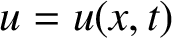 $u = u(x,t)$
satisfies the nonlinear system of PDEs
 $$ \begin{align} \displaystyle \frac{\partial u_i}{\partial t} = D \Delta u_i + f_i(u_1,u_2,\ldots,u_m) - D \frac{(1/\Phi_i'(y)) \nabla f_i(\Phi(y)) \cdot \Phi'(y) + \alpha}{f_i(\Phi(y))} \vert \nabla u_j \vert^2, \end{align} $$
for
 $i = 1,2,\ldots,m$
. The system (6.8) can then be used to construct upper and lower solutions provided a comparison principle exists for the system
 $\partial u/\partial t = D \Delta u + f(u)$
. The details are left to the reader.
7 Brief discussion and conclusion
In this paper, we considered the general Fisher–KPP equation in bounded domains with Dirichlet or homogeneous Neumann boundary conditions. Using the transformations between classes of nonlinear PDEs given in Section 2, we derived upper and lower solutions for the general Fisher–KPP equation. These comparison functions allowed us to obtain bounds for the critical times for this nonlinear RD equation. Previous results in the literature only considered either linear diffusion or linear RD equations.
Although this paper dealt with the critical times for the general Fisher–KPP equation, the upper and lower solutions given here may also be of use in other contexts, for example, in fisheries. Recall that a spatially homogeneous model for the growth of a species of fish under the effect of constant-effort harvesting can be given by
 $$ \begin{align*}\frac{du}{dt} = r u\, \bigg(1 - \frac{u}{K}\bigg) - E u, \end{align*} $$
where
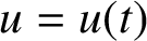 $u = u(t)$
is the species biomass at time t and
 $E \ge 0$
measures the effort spent in fishing. For example, E can be measured by the number of fishing boats at a given time. Suppose that
 $r> E$
. Then the steady states are
 $u_\infty = 0$
and
 $u_\infty = u_\infty (E) = K (1 - E/r)$
. It is straightforward to show that
 $u_\infty = 0$
is unstable while
 $u_\infty (E) = K (1 -E/r)$
is stable. The yield can be defined as
 $$ \begin{align*}Y(E) = E u_\infty(E) = K E - \frac{K}{r} E^2. \end{align*} $$
Then the yield is maximized when
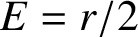 $E = r/2$
and the maximum yield is
 $Y(r/2) = r K/4$
. We deduce that increasing the effort E beyond
 $r/2$
is counterproductive as it decreases the yield.
If we extend this to the spatially heterogeneous case when
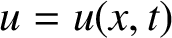 $u = u(x,t)$
, for example,
 $$ \begin{align*}\frac{\partial u}{\partial t} = D \Delta u + r u\, \bigg(1 - \frac{u}{K}\bigg) - E u, \end{align*} $$
then an equation of Fisher–KPP type arises. The steady state is now a (possibly) spatially heterogeneous solution
 $u_\infty = u_\infty (x;E)$
of the PDE
 $$ \begin{align*}D \Delta u_\infty + r u_\infty \bigg(1 - \frac{u_\infty}{K}\bigg) - E u_\infty = 0, \quad x \in \Omega, \end{align*} $$
with an appropriate boundary condition. We can define an analogue for the yield in the spatially heterogeneous case by a measure of the effort multiplied by the average limiting population distribution
 $$ \begin{align*}Y(E) = \frac{E}{m(\Omega)} \int_\Omega u_\infty(x;E) \, dx. \end{align*} $$
Another way is to fix
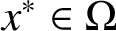 $x^* \in \Omega $
and define the yield as
 $Y(E) = E u_\infty (x^*;E)$
. We then use standard numerical optimization techniques to maximize
 $Y = Y(E)$
. Alternatively, using the upper solution
 $u^+ = u^+(x,t)$
and lower solution
 $u^- = u^-(x,t)$
constructed in Section 3, with
 $f(u) = r u (1 -u/k) - E u$
, we deduce that
 $u^-_\infty (x; E) \le u_\infty (x;E) \le u^+_\infty (x;E)$
for all
 $x \in \Omega \cup \partial \Omega $
, assuming that the initial biomasses are the same. As
 $$ \begin{align*}\frac{E}{m(\Omega)} \int_\Omega u^-_\infty(x;E) \, dx \le Y(E) \le \frac{E}{m(\Omega)} \int_\Omega u^+_\infty(x;E) \, dx, \end{align*} $$
we can therefore obtain bounds for the yield since
 $u_\infty ^\pm $
are known in principle.
Finally, the upper and lower solutions found here for the general Fisher–KPP equation do not seem to work for scalar RD equations with bistable nonlinearities, for example,
 $f(u) = u (1 - u) (u - a)$
for some
 $0 < a < 1$
. This is because in (2.7),
 $f(u)$
appears in the denominator and the last term becomes unbounded when
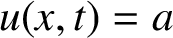 $u(x,t) = a$
.
A current work in progress is the investigation of moving boundary problems for the general Fisher–KPP equation. Using upper and lower solutions, such problems effectively reduce to studying moving boundary problems for nonlinear, but linearizable, PDEs. The underlying moving boundary problems for the corresponding linear PDEs (for example, (2.8)) can then be studied using the recent work by Rodrigo and Thamwattana [Reference Rodrigo and Thamwattana14] for analytically solving general fixed and moving boundary problems for the heat equation (1.1) considered on finite and infinite domains.