





1. Introduction
Turbulent particle-laden flows are widely encountered in various environmental and engineering applications. A vast majority of the literature on particle-turbulence interactions in wall-bounded flows is dedicated to the study of neutrally buoyant particles, where the mean particle slip velocity vanishes throughout the domain except in the wall region. A finite density ratio in the presence of gravity results in settling of particles, and the sustained wake region near the particles substantially alters the nature of particle–turbulence interaction. In the present work, we investigated the effect of slightly dense finite-size particles in vertical channel flows of Newtonian and viscoelastic carrier fluids using direct numerical simulations.
When the particle size is smaller or on the same order as the viscous dissipation length, turbulence modulation primarily depends on the Stokes number, defined as the ratio of particles to fluid response times (see Elghobashi (Reference Elghobashi2006), for regime classification based on the Stokes number). A gravitational acceleration decouples the particle's motion from the fluid, induces anisotropy in small scales and, as a result, has an immediate impact on turbulence modulation (Elghobashi & Truesdell Reference Elghobashi and Truesdell1993). It is known that small and heavy particles attenuate the turbulence intensity in homogeneous isotropic condition (Gore & Crowe Reference Gore and Crowe1989) as well as in turbulent channel flow (Tsuji, Morikawa & Shiomi Reference Tsuji, Morikawa and Shiomi1984). In the latter case the attenuation is particularly important in the cross-stream direction (Kulick, Fessler & Eaton Reference Kulick, Fessler and Eaton1994). At high particle concentrations, however, the strong interphase coupling triggers an alternative turbulence generation mechanism, where the turbulent kinetic energy is entirely generated by particles’ slip velocities (Capecelatro, Desjardins & Fox Reference Capecelatro, Desjardins and Fox2018). Particles motion is also influenced by gravity: in contrast to inertialess particles (or fluid elements) that are trapped inside eddies, dense particles escape the initially surrounding eddies faster than the eddy decay rate – a phenomenon known as ‘crossing trajectories’ which decreases particles’ dispersion due to the subdued correlated motions (Wells & Stock Reference Wells and Stock1983).
When the particle size lies in the inertial range of the turbulence, its wake interacts with turbulent eddies of different sizes (Cisse, Homann & Bec Reference Cisse, Homann and Bec2013). At particle Reynolds numbers  ${\textit {Re}}_p\equiv d_p u_{rms}/\nu \approx 20$ (where
 $\nu$,
 $d_p$ and
 $u_{rms}$ are the fluid kinematic viscosity, particle diameter and turbulent velocity fluctuations) the region of interaction extends to almost two particle diameters (Naso & Prosperetti Reference Naso and Prosperetti2010). Zeng, Balachandar & Najjar (Reference Zeng, Balachandar and Najjar2010) studied isolated stationary particles in turbulent channel flow for a wide range of particle Reynolds numbers based on the slip velocity (
 ${\textit {Re}}_p = 42\text {--}450$). The authors highlighted the dual effect of particles, where the turbulence kinetic energy is (i) suppressed due to the damping of the streamwise fluctuations and (ii) augmented by vortex shedding and/or wake oscillations. Towards the lower range of particle Reynolds numbers (
 ${\textit {Re}}_p \approx 26\text {--}33$), Vreman & Kuerten (Reference Vreman and Kuerten2018) considered a similar configuration and reported that particles create sinks of turbulence kinetic energy near their surfaces, although the turbulence suppression remains appreciable far from the particles. They concluded that the primary reason for turbulence suppression is particle-induced non-uniformity of the mean driving force of the flow, rather than turbulence modulations in the vicinity of the particles. At the higher particle Reynolds numbers (
 ${\textit {Re}}_p \approx 400$), Kajishima et al. (Reference Kajishima, Takiguchi, Hamasaki and Miyake2001) studied freely moving finite-size particles and investigated the influence of vortex shedding on turbulence production in a vertical channel.
At  ${\textit {Re}}_p \approx 136$ and low volume fractions
 $\varphi \approx 0.5\,\%$, Uhlmann (Reference Uhlmann2008) reported enhanced wall-normal mixing with flattening of the mean velocity profiles. They attributed the near-wall peak of particles concentrations to migration of particles in the direction opposite to gradients in the turbulence intensity – a phenomenon known as ‘turbophoresis’ (Caporaloni et al. Reference Caporaloni, Tampieri, Trombetti and Vittori1975). In a follow-up study, Garcia-Villalba, Kidanemariam & Uhlmann (Reference Garcia-Villalba, Kidanemariam and Uhlmann2012) examined the same configuration with a streamwise length twice as long, and they confirmed that particle and fluid statistics are not strongly affected by the streamwise extension of the domain, yet extremely long columnar flow structures remain correlated even at streamwise lengths of the order of
 $16h$, where
 $h$ is the channel half-width. Settling has also been examined in other canonical configurations including horizontal wall-bounded flows and homogeneous shear. In the former, Shao, Wu & Yu (Reference Shao, Wu and Yu2012) concluded that at high density ratios particles form a sediment layer over the horizontal wall, which contributes to the turbulence intensity by vortex shedding, and Kidanemariam et al. (Reference Kidanemariam, Chan-Braun, Doychev and Uhlmann2013) observed an apparent lag in the mean particle velocity compared with that of the fluid due to particle accumulation in the low-speed regions. When gravity is directed perpendicular to the plane of homogeneous shear, Tanaka (Reference Tanaka2017) concluded that the Reynolds shear stress is markedly decreased in the wake of particles and, in turn, the amplification of turbulent kinetic energy is reduced.
Another important implication of gravity and sustained particle wakes is the emergence of particle clusters. In quiescent flow conditions and at sufficiently large  ${\textit {Re}}_p$, the reduced drag acting upon trailing particles promotes cluster formation (Fortes, Joseph & Lundgren Reference Fortes, Joseph and Lundgren1987; Wu & Manasseh Reference Wu and Manasseh1998). This phenomenon has been extensively studied both experimentally (Huisman et al. Reference Huisman, Barois, Bourgoin, Chouippe, Doychev, Huck, Morales, Uhlmann and Volk2016) and numerically (Yin & Koch Reference Yin and Koch2007), and the onset of clustering is marked by a critical Galileo number which is defined as the ratio between gravitational and viscous forces (Uhlmann & Doychev Reference Uhlmann and Doychev2014). In the presence of background turbulence, Chouippe & Uhlmann (Reference Chouippe and Uhlmann2019) examined the clustering of finite-size particles in the presence of gravity, and highlighted that the background turbulence hinders cluster formation. Fiabane et al. (Reference Fiabane, Zimmermann, Volk, Pinton and Bourgoin2012) experimentally examined the clustering of finite-size particles, and concluded that a finite fluid/particle density difference is crucial for cluster formation. In a vertical turbulent channel, cluster formation induced by wake attraction is reported for particles with an unsteady wake (Kajishima Reference Kajishima2004), while particle distribution is reportedly more homogeneous than a random distribution when wake oscillations are absent (Garcia-Villalba et al. Reference Garcia-Villalba, Kidanemariam and Uhlmann2012). Overall, the influence of gravity on cluster formation is widely associated with the wake attraction mechanism, while the role of lateral forces in particles clustering and collective motion is less explored.
The literature on particle–turbulence interactions has predominately focused on Newtonian fluids. In absence of turbulence, particles in non-Newtonian flows have been studied (Zenit & Feng Reference Zenit and Feng2018), and the formation of particle-rich vertical columns has been observed in experiments of non-Brownian particles settling in a shear-thinning fluid (Bobroff & Phillips Reference Bobroff and Phillips1998; Mora, Talini & Allain Reference Mora, Talini and Allain2005). Once turbulence enters the picture, the vast literature on viscoelasticity (White & Mungal Reference White and Mungal2008; Samanta et al. Reference Samanta, Dubief, Holzner, Schäfer, Morozov, Wagner and Hof2013; Agarwal, Brandt & Zaki Reference Agarwal, Brandt and Zaki2014; Choueiri, Lopez & Hof Reference Choueiri, Lopez and Hof2018) has considered single-phase conditions for three reasons. Firstly, polymers have been among the most effective drag reduction technologies (Toms Reference Toms1948; Virk, Mickley & Smith Reference Virk, Mickley and Smith1970). Secondly, even single-phase viscoelastic flows exhibit puzzling dynamics that defy intuition based on Newtonian conditions. Examples include vorticity propagation as waves in viscoelastic flows (Page & Zaki Reference Page and Zaki2014), enstrophy amplification in two dimensions due to polymer torque (Page & Zaki Reference Page and Zaki2015, Reference Page and Zaki2016) and the initial destabilization of supercritical channel flow by increasing elasticity prior to its stabilization at higher Weissenberg numbers (Lee & Zaki Reference Lee and Zaki2017). The third reason is the lack of a mathematical framework that can facilitate progress in characterizing the state of polymers in turbulence. This point was addressed recently by a rigorous formulation for evaluating the mean conformation tensor (Hameduddin & Zaki Reference Hameduddin and Zaki2019) and quantifying departures from that mean (Hameduddin et al. Reference Hameduddin, Meneveau, Zaki and Gayme2018; Hameduddin, Gayme & Zaki Reference Hameduddin, Gayme and Zaki2019).
Building upon the above studies, it was recently possible to analyse the interplay of viscoelasticity, particles and turbulence for neutrally buoyant particles (Esteghamatian & Zaki Reference Esteghamatian and Zaki2019, Reference Esteghamatian and Zaki2020). In a viscoelastic channel flow at  $5\,\%$ particle concentration, particles periodically migrate away and towards the wall, while suppressing the turbulent activity, or reinforcing its hibernation. Viscoelasticity increased the formation of particle pairs with an angled alignment with respect to the streamwise direction, while no significant large-scale long-lived structure was identified (Esteghamatian & Zaki Reference Esteghamatian and Zaki2019). At
 $20\,\%$ particle concentration, a viscoelastic drag increase was reported for elasticity levels above a critical value. The enhanced polymer stress was attributed to strong deformations of polymers in the vicinity of particle surface (Esteghamatian & Zaki Reference Esteghamatian and Zaki2020).
In this work, we explore the settling effect of particles in vertical channel flow of Newtonian and viscoelastic fluids with direct numerical simulations. The particles are larger than the Kolmogorov length scale, and eddies at inertial ranges are expectedly affected by particles boundary layer and wake. Therefore, the computations resolve the flow at the scale of particles with an immersed boundary method, and the polymer forces are obtained by solving evolution equations for the polymer conformation tensor. The work explores the impact of gravity on the particle dynamics, fluid–particle coupling and the turbulent flow structures. Although the density ratio is modest, the findings are also relevant to the cluster-induced turbulence (known as CIT) regime. The flow configuration, governing equations and computational set-up are described in § 2. In § 3, we examine the impact of particle settling on multiple aspects of the channel flow dynamics including: the mean concentration and velocity profiles (§ 3.1); particle lift forces (§ 3.2); clusters and microstructure (§ 3.3); and momentum balance and velocity fluctuations (§ 3.4). Concluding remarks are provided in § 4.
2. Governing equations and numerical set-up
The computational domain is a plane channel, where the streamwise, wall-normal and spanwise directions are denoted  $x$,
 $y$ and
 $z$ (figure 1). The flow is maintained at a constant mass flux in the
 $x$ direction, and a gravitational field
 $\boldsymbol {g}$ acts in the opposite direction. The bulk velocity,
 $U_b$, and the channel half-height,
 $h$, are adopted as characteristic scales. The single-phase simulations are characterized by Reynolds number
 ${\textit {Re}} = hU_b/\nu$ and Weissenberg number
 $Wi = \lambda U_b/h$, where
 $\nu$ and
 $\lambda$ are the fluid total kinematic viscosity and the polymer relaxation time. The particle-laden configuration requires four additional dimensionless numbers: (i) dimensionless diameter of the particles
 $d_p/h$; (ii) density ratio between the particle and fluid phases,
 $\rho _r \equiv \rho _p/\rho _f$; (iii) bulk volume fraction
 $\varphi \equiv N_p \mathcal {V}_p/\mathcal {V}_t$, where
 $N_p$ is the number of particles,
 $\mathcal {V}_p$ is the volume of an individual particle and
 $\mathcal {V}_t$ is the volume of the computational domain; (iv) Froude number defined as
 ${\mathcal {F}r} =U^2_b/(|\boldsymbol {g}|h)$. The governing equations for the fluid velocity
 $\boldsymbol {u}_f$, the hydrodynamic pressure
 $p$ and the polymer conformation tensor
 $\boldsymbol{\mathsf{c}}$ in dimensionless form are
 \begin{gather} \boldsymbol{\nabla}\boldsymbol{\cdot}{\boldsymbol{u}_f} = 0, \end{gather}
 \begin{gather}\frac{\partial{\boldsymbol{u}_f}}{\partial{t}} + \boldsymbol{u}_f \boldsymbol{\cdot} \boldsymbol{\nabla}{\boldsymbol{u}_f}+\boldsymbol{\nabla}{p} - \frac{\beta}{Re} \nabla^{2}{\boldsymbol{u}_f} - \frac{1-\beta}{Re} \boldsymbol{\nabla}\boldsymbol{\cdot}{\boldsymbol{\mathsf{T}}} - \boldsymbol{F} = 0, \end{gather}
 \begin{gather}\frac{\partial{\boldsymbol{\mathsf{c}}}}{\partial{t}} +\boldsymbol{u}_f \boldsymbol{\cdot} \boldsymbol{\nabla}{\boldsymbol{\mathsf{c}}}- \boldsymbol{\mathsf{c}} \boldsymbol{\cdot} \boldsymbol{\nabla}{\boldsymbol{u}_f} - (\boldsymbol{\mathsf{c}} \boldsymbol{\cdot} \boldsymbol{\nabla}{\boldsymbol{u}}_f)^{\rm T} + \boldsymbol{\mathsf{T}} = 0. \end{gather}
In the above equations,  $\boldsymbol {F}$ is a generic force, and
 $\beta \equiv {\mu _s}/({\mu _s+\mu _p})$ is the ratio of solvent to total viscosity with the latter being comprised of the solvent
 $\mu _s$ and polymer
 $\mu _p$ contributions. For the present dilute polymer solution, the viscoelastic stress tensor
 $\boldsymbol{\mathsf{T}}$ is expressed in terms of the conformation tensor using the FENE-P model,
 \begin{equation} \boldsymbol{\mathsf{T}} \equiv \frac{1}{Wi} \left(\frac{\boldsymbol{\mathsf{c}}}{\psi}-\frac{{\boldsymbol{\mathsf{I}}}}{a} \right),\quad \psi = 1 - \frac{\text{tr}(\boldsymbol{\mathsf{c}})}{L^2_{max}},\quad a = 1- \frac{3}{L^2_{max}}, \end{equation}
where  ${\boldsymbol{\mathsf{I}}}$ is the isotropic tensor and
 $L_{max}$ is the maximum extensibility of the polymer chains. Particles’ motion in the presence of a gravitational field is governed by the Newton-Euler equations,
 \begin{gather} {\mathcal{V}_p} \frac{{\text{d}}{\boldsymbol{u}_p}}{\text{d}{t}} = \oint_{\partial {\mathcal{V}_p}} \boldsymbol{\sigma}_f \boldsymbol{\cdot} \boldsymbol{n} \text{d} \mathcal{A} + \boldsymbol{F}_c + \frac{1}{{\mathcal{F}r}}(\rho_r-1)\frac{\boldsymbol{g}}{|\boldsymbol{g}|}, \end{gather}
 \begin{gather}\mathcal{I}_p \frac{{\text{d}}{\boldsymbol{\varOmega}_p}}{\text{d}{t}} = \oint_{\partial {\mathcal{V}_p}} \boldsymbol{r} \times \boldsymbol{\sigma}_f \boldsymbol{\cdot} \boldsymbol{n} \,\text{d} \mathcal{A}, \end{gather}
 \begin{gather}\boldsymbol{\sigma}_{f} ={-}p{\boldsymbol{\mathsf{I}}} + 2\frac{\beta}{{\textit{Re}}}{\boldsymbol{\mathsf{E}}} + \frac{1-\beta}{{\textit{Re}}} \boldsymbol{\mathsf{T}}, \end{gather}
where  $\boldsymbol {u}_p$,
 $\boldsymbol {\varOmega }_p$,
 ${\mathcal {V}_p} = {{\rm \pi} d_p^3}/{6}$ and
 ${\mathcal {I}_p}= {{\rm \pi} d_p^5}/{60}$ are the translational and angular velocities and dimensionless volume and moment of inertia of a spherical particle, and
 ${\boldsymbol{\mathsf{E}}}$ is the strain-rate tensor of the fluid phase. The hydrodynamic stress tensor,
 $\boldsymbol {\sigma }_f$, is integrated over a particle's surface, and
 $\boldsymbol {n}$ denotes the outward unit vector normal to that surface. The particle–particle and particle–wall repulsive collision forces,
 $\boldsymbol {F}_c$, are applied in the opposite direction to
 $\boldsymbol {n}$, and the last term on the right-hand side of (2.5) accounts for the buoyancy force.
Schematic of the particle-laden simulations. No-slip boundary conditions  $\boldsymbol {u}_f = 0$ are imposed at
 $y = \{0, 2\}$, and periodicity is enforced in the
 $x$ and
 $z$ directions.

A complete description of our numerical algorithm is provided by Esteghamatian & Zaki (Reference Esteghamatian and Zaki2019) and, for completeness, only the main features are described here. The flow equations, (2.1) and (2.2), were solved using a fractional step algorithm on a staggered grid with a local volume-flux formulation (Rosenfeld, Kwak & Vinokur Reference Rosenfeld, Kwak and Vinokur1991), and the conformation-tensor equations, (2.3), were solved using a third-order accurate Runge–Kutta method. The viscous terms were solved implicitly in time using the Crank–Nicolson scheme, while an explicit Adams–Bashforth scheme is adopted for advection and stretching terms in (2.2) and (2.3). Following Dubief et al. (Reference Dubief, Terrapon, White, Shaqfeh, Moin and Lele2005), a semi-implicit approach that ensures the finite extensibility of the polymers was used to discretize the polymer stress term. In particle-laden cases, a sharp-interface immersed boundary force field (Nicolaou, Jung & Zaki Reference Nicolaou, Jung and Zaki2015) enforces the no-slip boundary condition at the surface of the particles ( $\boldsymbol {F} = \boldsymbol {F}_{{IB}}$ in (2.2)), and the conformation tensor is set to unity inside the particle domain. The short-range particle–particle and particle–wall collision model introduced by Glowinski et al. (Reference Glowinski, Pan, Hesla, Joseph and Périaux2001) is adopted, which is activated at gap distances smaller than the diagonal of the fluid grid cell. The algorithm has been extensively validated for simulations of Newtonian and viscoelastic flows (Lee & Zaki Reference Lee and Zaki2017; Wang, Wang & Zaki Reference Wang, Wang and Zaki2019b) including particle-laden conditions (Esteghamatian & Zaki Reference Esteghamatian and Zaki2019, Reference Esteghamatian and Zaki2020).
The set of physical parameters are selected such that they demonstrate the effect of settling on the dynamics of the flow and particles. The simulations will contrast dense particles in Newtonian and viscoelastic fluids (designated ‘W0P5D’ and ‘W15P5D’) to neutrally buoyant conditions (‘W0P5’ and ‘W15P5’) and single-phase flows (‘W0’ and ‘W15’). In the designation, ‘W’ refers to the Weissenberg number which is either  $Wi=0$ for Newtonian or
 $Wi=15$ for viscoelastic flow; ‘P’ refers to the presence of a particle phase with bulk particle volume fraction
 $\varphi = 5\,\%$; ‘D’ indicates dense particles. In the Newtonian single-phase configuration, the friction Reynolds number
 ${\textit {Re}}_\tau \equiv hu_\tau /\nu \approx 180$, where
 $u_\tau \equiv \sqrt {\langle \tau _{w} \rangle /\rho }$ denotes the friction velocity and
 $\langle \tau _{w} \rangle$ is the average wall shear stress. The dimensionless particle diameter is
 $d_p/h = 1/9$, and in viscous scaling they lie in the range
 $20 \le d^+ \le 32$. With a particle response time based on Stokes drag,
 $t_p \equiv {d_p}^2 \rho _p/18\mu$, the Stokes number is
 $St\equiv h t_p/U_b \sim O(1)$ or
 $St^+\equiv t_pu^2_\tau /\nu \sim O(10)$. Interaction between the fluid and particle phases is, therefore, expected. Despite the mild density ratio (
 $\rho _r=1.15$) in dense cases, the settling effect is substantial, and the particle Reynolds number defined based on the slip velocity,
 ${\textit {Re}}_p \equiv d_p (u_p-u_f) / \nu$, is on average
 ${\textit {Re}}_p \approx 130$ in W0P5D and
 ${\textit {Re}}_p\approx 95$ in W15P5D. The Galileo number is defined by the ratio of viscous and gravitational forces,
 $Ga \equiv (|\rho _r-1|d_p|\boldsymbol {g}|)^{1/2} d_p/\nu = 126$ for the dense particles, and a steady vertical particle wake is anticipated (Uhlmann & Doychev Reference Uhlmann and Doychev2014). A list of physical and computational parameters is provided in table 1.
Physical and computational parameters of the simulations. Reynolds number  ${\textit {Re}} \equiv hU_b/\nu$ and Weissenberg number
 $Wi \equiv \lambda U_b/h$ are based on the channel half-height
 $h$, the bulk velocity
 $U_b$, total kinematic viscosity
 $\nu$ and viscoelastic fluid relaxation time
 $\lambda$. The domain sizes are
 $L_{\{x,y,z\}}$ in
 $\{x,y,z\}$ directions, and the numbers of grid cells are
 $N_{\{x,y,z\}}$.

A uniform Cartesian grid was used in all three directions in the particle-laden simulations. In the single-phase cases, the grid spacing was uniform in the spanwise and streamwise dimensions, and a hyperbolic tangent grid stretching was adopted in the wall-normal direction. The domain size was  $6\times 2 \times 3$ in streamwise, wall-normal and spanwise directions in single-phase and neutrally buoyant particle-laden cases, while in dense particle-laden cases the domain size was extended to
 $8\times 2 \times 4.5$. The grid size was set to
 $d_p/ {\rm \Delta} x=16$ in all particle-laden conditions. Beyond the initial transient, statistics were collected for sufficiently long periods (e.g. 900 convective time units for case W0P5D), and convergence was verified by comparing results from half the number of samples, and the total number of samples. For a generic variable
 $o$, phase-averaged statistics are related to unconditional counterparts with a phase indicator
 $\chi$ that is zero in the fluid and unity in the particle phase,
 \begin{equation} \langle o\rangle =\langle (1-\chi)o_f\rangle + \langle \chi o_p\rangle = (1-\phi)\langle o_f \rangle_f + \phi \langle o_p \rangle_p, \end{equation}
where  $\phi$ denotes the particle volume fraction. For brevity, the subscripts
 $\{\,f,p\}$ are hereafter omitted from the averaging symbol. Unless otherwise stated, the averaging operation is performed in time and in homogeneous
 $x$ and
 $z$ directions.
3. Results
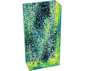
An instantaneous field from the Newtonian dense-particle-laden case (W0P5D) is shown in figure 2 which highlights key features that are exclusive to the dense particle cases. Collective particle motion is evident from their large-scale velocity structures. Wakes downstream of individual particles highlight the potential impact on the collective motion and cluster formation. Particle motion affects the fluid-phase streamwise velocity structures as shown by contours of  $u_f$, both at a microscale due to the finite slip velocities, and at a global scale due to the collective motion. Since the flow is dominated by particles, we start by investigating the mechanisms controlling the particles motion. Subsequently, a discussion on the impact of gravity and particle wakes on the mean stress balance and fluid fluctuations is provided.
(a) Instantaneous snapshot of particle positions coloured by their velocity and contours of  $u_f$ for case W0P5D. For clarity only particles located at
 $y \le 1$ are displayed. (b) A subset of the domain is magnified and reproduced with isosurfaces of
 $u_f=0.7$. (c) Contours of
 $u_f/\langle u_f \rangle$ in the
 $(x,y)$ plane in the vicinity of one particle.

3.1. Particle concentration and mean velocity profiles
Multiple physical mechanisms that distinguish dense particle cases from neutrally buoyant counterparts are direct consequences of the relative velocity of the particles with respect to the fluid. As shown in figures 3(a) and 3(d), the particles sustain a negative relative velocity and as a result a positive drag that counterbalances the buoyancy force exerted in the negative  $x$ direction. Since the buoyancy force is constant at all
 $y$ locations, the particle slip velocity
 $\langle u_p \rangle - \langle u_f \rangle$ is nearly constant across the bulk of the flow. The smaller magnitude of
 $\langle u_p \rangle - \langle u_f \rangle$ in the viscoelastic case W15P5D compared with the Newtonian fluid W0P5D suggests that particles experience a larger drag coefficient in the former, in agreement with previous studies (Chhabra Reference Chhabra2006).
Profiles of average (a,d) particle velocity relative to the fluid, (b,e) particle concentration and (c,f) fluid velocity. Suspensions: neutrally buoyant (circle – line, black), dense particles (filled circle – line, black); single-phase condition (—–, blue). The fluid in panels (a–c) is Newtonian and in panels (d–f) is viscoelastic. Vertical dashed lines in panels (b,c) and panels (e,f) mark the locations of the peak particles concentration.

The concentration profiles of neutrally buoyant and dense particles are reported in figure 3(b) for Newtonian fluid and in figure 3(e) for the viscoelastic case. In the latter, neutrally buoyant particles migrate towards the channel centre due to imbalance of elastic normal stresses (D'Avino & Maffettone Reference D'Avino and Maffettone2015). For dense particles, the repulsion away from the wall is enhanced for  $y \le 0.2$, and the absence of mean shear beyond
 $y=0.2$ eliminates particle migration towards the centre. The presence of a local maximum near
 $y=0.2$ for the dense particle cases, both viscoelastic and Newtonian, is remarkable. This peak is qualitatively different to the relatively small maximum in
 $\phi$ that is discernible in the viscoelastic neutrally buoyant case that was previously attributed to the lubrication forces and the asymmetric interparticle interactions (Esteghamatian & Zaki Reference Esteghamatian and Zaki2019). That mechanisms cannot explain the strong local maximum in dense cases, where the immediate vicinity of the wall (
 $y < d_p$ in the case W15P5D) is almost void of particles. Similar patterns were typically attributed to the turbophoretic forces (Reeks Reference Reeks1983) for point particles (Kaftori, Hetsroni & Banerjee Reference Kaftori, Hetsroni and Banerjee1995; Marchioli & Soldati Reference Marchioli and Soldati2002) and small particles with size
 $d^+_p\approx 5\text {--}10$ (Garcia-Villalba et al. Reference Garcia-Villalba, Kidanemariam and Uhlmann2012). In that regime, lift forces are also important as noted in theoretical (Young & Leeming Reference Young and Leeming1997) and numerical studies (Marchioli, Picciotto & Soldati Reference Marchioli, Picciotto and Soldati2007; Wang et al. Reference Wang, Fong, Coletti, Capecelatro and Richter2019a). For particles much larger than the Kolmogorov scale, Kajishima et al. (Reference Kajishima, Takiguchi, Hamasaki and Miyake2001) underscored the influence of lift forces on particles’ motion in homogeneous turbulence. Another interesting case is vertical bubble-laden channel flow where the slip velocities are positive, and hence opposite to the present configuration with dense particles. In that case, wallward lift forces migrate the bubbles from the channel interior to form a bubble-rich layer near the wall (Lu & Tryggvason Reference Lu and Tryggvason2013). Here, we will investigate the role of shear- and rotation-induced lift in clustering of large settling particles (
 $d^+\approx 30$).
The strong repulsion from the wall is due to the Saffman lift force (Saffman Reference Saffman1965), and can be expressed as  $F_\text {S} \equiv -C_l \rho _f \sqrt {\nu } d_p^2 (u_p-u_f) \dot {\gamma }/\sqrt {|\dot {\gamma }|}$, where
 $\dot {\gamma }$ is the shear rate and
 $C_l$ is a constant coefficient. Other forms of the Saffman lift account for finite Reynolds number and wall effects (Leighton & Acrivos Reference Leighton and Acrivos1985; Mei Reference Mei1992; Zeng et al. Reference Zeng, Najjar, Balachandar and Fischer2009), but they do not influence the direction of the lift force which is the relevant element here. The negative sign of
 $\langle u_p \rangle - \langle u_f \rangle$ in W0P5D and W15P5dD gives rise to a Saffman lift force displacing the particles away from the immediate vicinity of the wall – an effect that is insignificant in the neutrally buoyant cases due to the inappreciable relative velocity. Nonetheless, the Saffman lift force alone cannot fully explain the peak in the particle concentration profile. As will be discussed further in this section, the presence of the peak is related to the coupling of angular and translational velocities of dense particles.
The fluid velocity profiles are significantly different for dense particles than neutrally buoyant, and the change is accentuated in the viscoelastic case. Due to the reaction of the particle drag forces on the fluid field, the flow slows down in the channel core. The mean velocity is nearly flattened in the bulk, in a stark contrast to the W15P5 where the velocity tends to the Poiseuille profile. Near the walls ( $y\approx \{0.1, 0.15\}$ for W0P5D and W15PD), the fluid speeds up avoiding the resistive forces from the particles in the bulk. As a result, in both the viscoelastic and Newtonian cases, a local maximum in fluid velocity is observed between the wall and the peak in the particle concentration.
We now direct our attention on the angular particle velocities, which play an important role in the global dynamics of the suspension (figure 4). The correlation between particles’ angular velocity and the local fluid vorticity has been previously investigated in linear shear flows (Ding & Aidun Reference Ding and Aidun2000) and turbulent channels (Uhlmann Reference Uhlmann2008). Neutrally buoyant particles sustain a negative spanwise angular velocity  $\varOmega _{p,z}$ throughout the bottom half of the channel, similar to the negative mean spanwise vorticity
 $\varOmega _{f,z}$. In the dense particle cases,
 $\varOmega _{p,z}$ vanishes away from the walls, is positive over a short wall-normal extent and reaches large negative values in the vicinity of the wall. The region of positive mean vorticity occurs below the peak in the particle concentration profile, for instance over
 $0.12 \le y \le 0.15$ when the peak of
 $\phi$ is at
 $y=0.16$ in W0P5D. That positive vorticity is thus associated with the shear layer generated at the edge of the high concentration of particles moving much slower than the mean flow. The particles naturally experience positive angular velocity at this location. Interestingly, they preserve this positive velocity closer to the wall where vorticity becomes negative (see the inset of figures 4b and 4d). This observation highlights that the positive angular velocity of the dense particles near the wall cannot only be explained by the local positive fluid vorticity; other physical mechanisms are at play.
Profiles of average spanwise (a,c) fluid vorticity and (b,d) particle angular velocity. Suspensions: neutrally buoyant (circle – line, black), dense particles (filled circle – line, black); single-phase condition (—–, blue). The fluid in the panels (a,b) is Newtonian and in panels (c,d) is viscoelastic. The marked area is magnified in the inset, and shaded area in the inset of panels (b,d) indicates the  $y$ locations where
 $\langle \varOmega _{f,z}\rangle >0$.

To further investigate this matter, conditional statistics of particles with positive and negative spanwise angular velocities are shown in figure 5. The conditioned wall-normal particle flux demonstrates a clear dependence on its angular velocity (figures 5a and 5c): particles which rotate in the positive  $z$ direction experience wallward velocities and vice versa. As a result, mostly particles with a positive angular velocity can penetrate into the region
 $y \le 0.2$ and, therefore, the unconditional average particle angular velocity is positive in that region (figures 4b and 4d). Confirming this trend, figures 5(b) and 5(d) show that the volume fraction of particles with
 $\varOmega _{p,z}>0$ is significantly larger near the wall. The coupling of angular and translational velocities also provides an explanation for the unconditional particle concentration profile: away from the walls, particles efficiently mix in the wall-normal direction due to the equal positive and negative fluxes
 $\langle v_{p} \rangle \phi$ associated with positive and negative rotation. As a result, profiles of
 $\phi$ are flat for
 $y \ge 0.3$ in both W0P5D and W15P5D cases. Near the wall, a strong peak in
 $\phi$ is observed, which is established primarily by particles with
 $\varOmega _{p,z}>0$ and
 $v_p<0$. The wallward flux of these particles is halted by the near-wall repulsive lift forces, and as a result the peak concentration is established.
Profiles of conditionally averaged (a,c) wall-normal particle flux and (b,d) particle concentration. Here  $\varOmega _{p,z} > 0$ (—–, red);
 $\varOmega _{p,z} < 0$ (- - - - -, blue); unconditional statistics (– – –, black). The fluid in panels (a,b) is Newtonian and in panels (c,d) is viscoelastic.

The coupling of angular and translational velocities hints to the relevance of rotation-induced lift forces (Magnus Reference Magnus1853). Nonetheless, due to the additive nature of hydrodynamic forces, isolating individual contributions is not a trivial task. In the following section, ensemble averages along particle trajectories are investigated to elucidate the hydrodynamic effects that control the motion of particles.
3.2. Ensemble averages along particle trajectories
Hydrodynamic forces acting perpendicular to the primary direction of motion of a sphere are broadly divided into shear- and rotation-induced contributions. In the limit of small and high particle Reynolds numbers, the shear-induced lift is the first-order contribution and the influence of rotation-induced lift is deemed to be negligible. For an intermediate range of the particle Reynolds numbers, approximately from 5 to 100, particle's free rotation has a measurable impact on its motion (Bagchi & Balachandar Reference Bagchi and Balachandar2002). In our dense particle cases, the average particle Reynolds number is  ${\textit {Re}}_p \approx \{130, 95\}$ in the Newtonian and viscoelastic conditions and, therefore, the rotation-induced lift force is expected to be important.
We exploit the absence of mean shear in the span to highlight the effect of rotation-induced lift force, by investigating the particle trajectories projected onto the  $xz$ plane (figure 6). Particles with positive and negative
 $\varOmega _{p,y}$ are tracked for approximately 10 time units in the Newtonian cases. Evidently, the sign of
 $\varOmega _{p,y}$ is a predictor of dense particles’ direction of motion in the span, while the neutrally buoyant particles disperse randomly regardless of their angular velocity. Similar trends in the trajectories are observed in the viscoelastic cases (not shown for brevity).
Sample particle trajectories projected onto the  $xz$ plane for particles with a positive (—–, red) or negative (—–, blue) wall-normal angular velocity
 $\varOmega _{p,y}$; (a) W0P5 (b) W0P5D. Particles velocity relative to the fluid is in the negative
 $x$ direction and the positive
 $y$ axis points into the page. All particles are located at approximately the same
 $z$ location at the beginning of the observation time window, during which
 $\varOmega _{p,y}$ does not change sign.

Ensemble-averaged properties along the trajectories are denoted  $\langle \cdot \rangle _{tr}$, and are plotted for W0P5D and W15P5D cases (figure 7). The averaging is conditioned on the sign of
 $\varOmega _{p,y}$ at
 $t_0$, where
 $t_0$ denotes the time at which the condition is satisfied, and the statistics are plotted versus
 $t' \equiv t-t_0$. In an inviscid laminar flow, the Magnus lift force is expressed as
 $\boldsymbol {F}_{Mag} = C_{lm} d_p^2 \rho _f \boldsymbol {\varOmega }_p \times (\boldsymbol {u}_p-\boldsymbol {u}_f)$ (Auton, Hunt & Prud'Homme Reference Auton, Hunt and Prud'Homme1988). Therefore, for the present conditions where particles are moving slower than the mean flow in the streamwise direction, when
 $\boldsymbol {\varOmega }_p$ is aligned with the positive
 $y$ axis the Magnus lift force is in the positive
 $z$ direction. In both Newtonian and viscoelastic conditions, figure 7 shows that the spanwise translational velocity is positively correlated with the wall-normal angular velocity, which confirms the relevance of the Magnus lift forces. Interestingly, the peak in the hydrodynamic force, which is induced by the Magnus effect, precedes the particles’ maximum angular and translational velocities. In fact,
 $\langle F_{h,z} \rangle _{tr}$ sharply decreases and changes sign approximately between
 $-1 \le t' \le 1$. When a particle begins to gain momentum in the
 $z$ direction due to the Magnus force, the surrounding fluid resists the particle's motion, and the particle experiences a drag force counteracting the Magnus lift. Finally, while the importance of the Magnus lift force in particles’ motion is evident in both Newtonian and viscoelastic conditions, in the latter case has smaller magnitudes of both the translational and angular velocities and of the hydrodynamic force.
Ensemble-averaged properties along the trajectories  $\langle \cdot \rangle _{tr}$ for particles with a positive (—–, red) or negative (- - - - -, blue) wall-normal angular velocity
 $\varOmega _{p,y}$ at
 $t_0$, where
 $t_0$ denotes the time at which the condition is satisfied; (a) W0P5D (b) W15P5D. The shifted time is denoted
 $t'\equiv t-t_0$, and the particle properties from top to bottom are wall-normal angular velocity, spanwise translational velocity and spanwise hydrodynamic force exerted on the particle and normalized by the particle buoyancy force
 $F_b\equiv (\rho _p-\rho _f)V_p|\boldsymbol {g}|$. Particles are located within
 $0.4 \le y \le 1$ at
 $t'=0$.

We now turn to the  $xy$ plane, where sample particle trajectories are plotted in figure 8 for W0P5D; this time the trajectories are conditioned on the spanwise angular velocity of the particles. As noted earlier in § 3.1, a shear-induced lift force repels the particles away from the wall. Similar to their spanwise motion, the wall-normal motion of dense particles is also correlated to their angular velocity. Particles with
 $\varOmega _{p,z}<0$ migrate towards the centre of the channel while particles with positive rotation penetrate towards the wall. Nonetheless, due to the strong shear-induced lift force away from the wall, it is very unlikely that the particles directly interact with the wall.
Sample particle trajectories projected onto the  $xy$ plane for particles with a positive (—–, red) or negative (—–, blue) spanwise angular velocity
 $\varOmega _{p,z}$ in W0P5D. Particles velocity relative to the fluid is in the negative
 $x$ direction and the positive
 $z$ axis points out of the page. All particles are located at approximately the same
 $y$ location at the beginning of the observation time window, during which
 $\varOmega _{p,z}$ does not change sign. The solid grey line marks the geometric limit for particles centre in
 $y$ direction.

For particles located within  $y \le 0.4$, ensemble averages along particle trajectories are shown in figure 9. It should be noted that due to the rotation-induced lift force, the likelihood of presence of particles with
 $\varOmega _{p,z}<0$ in the region
 $y \le 0.4$ is low and, as a result,
 $\varOmega _{p,z}$ is on average positive within
 $y \le 0.4$ (see figures 4b and 4d). Thus, even for those particles with
 $\varOmega _{p,z}<0$, it is more likely that their spanwise angular velocity has changed sign shortly before
 $t'=0$ (the top row of figure 9). After
 $t'>0$, however, particles have already reached the vicinity of the wall, and the strong negative fluid vorticity drives their angular velocities to negative values. Similarly, particles experience negative wall-normal velocity before
 $t'=0$ and positive values after (the middle row of figure 9). At
 $t'=0$, the effect of the Magnus effect is more evident: particles with positive spanwise angular velocity experience negative wall-normal velocity, and vice versa. Investigating the ensemble-averaged hydrodynamic forces is complex, as one should account for simultaneous effects of shear- and rotation-induced lift forces, as well as the resistive drag force opposing any incurred motion (the bottom row of figure 9). For particles with
 $\varOmega _{p,z}<0$, the shear- and rotation-induced forces are both in the positive
 $y$ direction and, therefore, the particles experience a strong force towards the channel centre when
 $t' < 0$. Their motion away from the wall is resisted by drag, resulting in vanishing net force when
 $t'>0$. For particles with
 $\varOmega _{p,z}>0$, the shear- and rotation-induced lift forces are in opposite directions, and the net effect is a force in positive
 $y$ direction with a weaker peak compared with the particles with
 $\varOmega _{p,z}<0$.
Ensemble-averaged properties along the trajectories  $\langle \cdot \rangle _{tr}$ for particles with a positive (—–, red) or negative (- - - - -, blue) spanwise angular velocity
 $\varOmega _{p,z}$ at
 $t_0$, where
 $t_0$ denotes the time at which the condition is satisfied; (a) W0P5D (b) W15P5D. The shifted time is denoted
 $t'\equiv t-t_0$, and the particle properties from top to bottom are spanwise angular velocity, wall-normal translational velocity and wall-normal hydrodynamic force exerted on the particle and normalized by the particle buoyancy force
 $F_b\equiv (\rho _p-\rho _f)V_p|\boldsymbol {g}|$. Particles are located within
 $y \le 0.4$ at
 $t'=0$.

3.3. Clustering, microstructure and particle wake
We have seen that the presence of gravity gives rise to sustained slip velocities, lift forces and significant changes in the mean profiles. The statistical averaging, however, masks the impact of gravity on the spatial distribution, or clustering, of particles in the wall-parallel planes. In this section, we examine the particles’ collective motion and potential clustering effects, and relate these macroscale observations to the microscale dynamics, e.g. lift forces, microstructure and particle wake.
The Voronoï diagram (Okabe et al. Reference Okabe, Boots, Sugihara and Chiu2000) has previously been used to examine clustering in particle-laden turbulent flows (Monchaux, Bourgoin & Cartellier Reference Monchaux, Bourgoin and Cartellier2010; Garcia-Villalba et al. Reference Garcia-Villalba, Kidanemariam and Uhlmann2012), and will be adopted herein for cluster analysis. The domain, either a plane or a volume, is partitioned into  $n$ cells marking the neighbouring region of
 $n$ particles, i.e. the
 $i$th particle centre is the closest particle centre to all of the points that belong to the
 $i$th cell. Two examples of Voronoï tessellations are shown in figure 10: the first is in a plane based on particles’ centres near the wall, and the second is in a volume for particles near the channel centre. Isolated particles are located in larger cells, while smaller cells indicate high particle concentrations. For the near-wall particles clustering is visually discernible in this particular instance of the flow.
Voronoï tessellation of (a) the  $xz$ plane located at
 $y = 3d_p/4$ and (b) the volume
 $0.8 \le y \le 1.2$ corresponding to one snapshot of particle centres in W0P5D. In panel (b) only a subset of the domain is visualized for the sake of clarity.

A quantitative assessment of clustering is provided by evaluating the probability density function (p.d.f.) of normalized surface areas of Voronoï cells (figure 11). The position of particles located in a wall-parallel bin are projected onto the  $xz$ plane. The extent of the bin in the wall-normal direction is
 $d_p/2$, while in the
 $x$ and
 $z$ directions it spans the full domain. The bin is placed at the closest location to the wall with a statistically significant number of particles,
 $y = 5d_p/4$ in W15P5D and
 $y=3d_p/4$ in all other cases, and we denote this volume as the ‘wall region’. In all cases, the local particle volume fraction within the wall region is approximately
 $25\,\%$ of the bulk value. The width of the p.d.f. highlights the heterogeneity of the particles distribution, and its tails indicate the likelihood of finding clustered and isolated particles. For example, for a uniformly structured layout of particles the area of Voronoï cells are all equal and, therefore, the p.d.f. becomes a Dirac function. For each case, the results for a random distribution of non-overlapping particles with a matching particle volume fraction is also presented as a reference. For neutrally buoyant particles the differences between the p.d.f.s of normalized Voronoï areas for the present data and a random distribution are statistically insignificant. In the case of dense particles in both Newtonian and viscoelastic fluids, however, the p.d.f.s (a) have thicker tails and (b) their peaks are shifted towards smaller values of
 $\mathcal {A}/\langle \mathcal {A} \rangle$ in comparison with a random distribution. The former observation highlights the high probability of finding significantly clustered and isolated particles, and the latter point indicates that the particles are more likely to be in close proximity of one another. Both conclusions are in agreement with the aggregating patters visually seen in the sample snapshot (figure 10a).
The p.d.f. of normalized Voronoï cell areas for particles in the wall region, i.e.  $d_p \le y \le 1.5d_p$ in W15P5D and
 $0.5d_p \le y \le d_p$ in all other cases; (a) W0P5, (b) W0P5D, (c) W15P5, (d) W15P5D. For each case, p.d.f. of the same quantity is also plotted for a random distribution of non-overlapping particles with a matching particle volume fraction (grey dashed lines (- - -)).

Clustering in turbulent flows is often due to the preferential accumulation of particles in coherent turbulent structures (Kaftori et al. Reference Kaftori, Hetsroni and Banerjee1995). Nevertheless, clustering by turbulence is only observed for small particles ( $d^+ < 10$) (Hetsroni & Rozenblit Reference Hetsroni and Rozenblit1994) and is, therefore, not relevant in our cases where
 $d^+ \approx \{28, 32\}$ for W0P5D and W15P5D. In a non-uniform distribution of particles, and in fact even in a homogeneous random distribution, some particles reside in more aggregated regions while others are relatively isolated. The same applies to the non-uniform particle distribution in the subvolume
 $d_p < y \le 2d_p$, which is adjacent to the wall region. We argue that the observed clustering in the
 $xz$ plane is due to the preferential transport of aggregated particles from
 $d_p<y \le 2d_p$ towards the wall region, i.e.
 $0.5d_p \le y \le d_p$. In other words, the wallward transport is less likely for isolated particles and, therefore, the wall region consists mostly of aggregated ones. In § 3.1 we showed that the particles experience positive spanwise angular velocities when located within
 $y \le 0.2$ (figures 4b and 4d) and, therefore, are pushed towards the wall by a rotation-induced lift force. Why this effect favours aggregated particles is shown schematically in figure 12(a). The slip velocity of the particles results in shear layers, with positive and negative vorticities on either side, and the same effect applies to the aggregate. For isolated particles, the net effect is a weak rotation-induced lift force towards the wall. On the other hand, for particles within the aggregate, the effect is most substantial: particles in the wall-facing edge of the aggregate experience strong positive vorticity due to the near-wall accelerated fluid, while being shielded from the negative vorticity by neighbouring particles. As a result, they attain a large positive angular velocity and, in turn, experience a strong rotation-induced lift force towards the wall.
(a) Schematic of the rotation-induced lift forces acting on the aggregated and isolated particles within  $d_p<y \le 2d_p$, and the preferential transport of aggregated particles towards the wall. (b) The p.d.f. of normalized Voronoï cell areas
 $\mathcal {A}/\langle \mathcal {A} \rangle$ for case W0P5D and particles located at
 $y \le d_p$. The data are conditioned based on
 ${\rm \Delta} t\equiv t-t_e$, where
 $t_e$ denotes the time at which a particle entered
 $y \le d_p$ and
 $t$ is the time of data collection. The red dashed line (- - -) is the unconditional p.d.f. and the grey dashed line (- - -) shows the p.d.f. for a random distribution of non-overlapping particles. Note that the average Voronoï cell area
 $\langle \mathcal {A}\rangle$ is not conditioned. The shaded area shows the range of
 $\mathcal {A}/\langle \mathcal {A} \rangle$ for which the particles are clustered.

It is important to highlight another mechanism that contributes to the preferential transport of aggregated particles towards the wall. As will be discussed shortly, aggregated particles experience enhanced slip velocities and, therefore, a more substantial wake, compared with the isolated ones. The intensified wake of aggregated particles enhances the lift forces, leading to higher likelihood of penetrating towards the wall and, as a result, strong clustering effect is observed in that region.
For further evidence of the preferential wallward migration of aggregated particles, we revisit the p.d.f. of  $\mathcal {A}/\langle \mathcal {A}\rangle$ for particles within
 $y \le d_p$ (figure 12b). This time, however, we condition the data with respect to
 ${\rm \Delta} t \equiv t-t_e$, where
 $t_e$ denotes the time at which the particle enters
 $y \le d_p$ region and
 $t$ is the time of data collection. Results are shown only for W0P5D and similar trends are also observed in W15P5D. Two additional curves are plotted (dashed curves), the unconditional p.d.f. for the present data and of a random distribution of non-overlapping particles, and the first intersection of these two curves is a measure that identifies clustering (Monchaux et al. Reference Monchaux, Bourgoin and Cartellier2010). The p.d.f. for
 ${\rm \Delta} t =0$ represents the particles that entered
 $y \le d_p$ region from the adjacent subvolume, i.e.
 $d_p<y \le 2d_p$, at the time of data collection. For those particles, the probability of being in a cluster is higher than the rest of the particles. As
 ${\rm \Delta} t$ increases, the p.d.f.s of conditional data tends to that of the unconditional curve, except in the extremely clustered range of the distribution (
 $\mathcal {A}/\langle \mathcal {A} \rangle \le 0.1$). Interestingly, in that range the conditional p.d.f.s move away from that of the unconditional data with increasing
 ${\rm \Delta} t$, implying that only the particles which recently penetrated the wall region can experience extreme clustering. Overall, it is concluded that the clusters are transported from the adjacent subvolume
 $d_p<y \le 2d_p$ rather than being formed in the wall region itself.
The increase in local particle concentration has been tied to enhanced particle settling velocity in homogeneous isotropic turbulence (Aliseda et al. Reference Aliseda, Cartellier, Hainaux and Lasheras2002). In our vertical channel configuration, figure 13 demonstrates the impact of clustering on the particles streamwise velocities. A correlation is observed between  $u_p-\langle u_p \rangle$ and
 $\log _{10}(\mathcal {A}/\langle \mathcal {A} \rangle )$ for the dense particles only. Particles in clusters have smaller streamwise velocities compared with the isolated ones and, as a result, larger slip velocities. In all dense particle cases the slip velocity is inversely proportional to the drag coefficient, since the particle's drag is balanced by the buoyancy force which is constant across the channel. Therefore, larger slip velocities in clusters imply that the aggregated particles experience a reduced drag coefficient due to the sheltering effect of neighbouring particles. This phenomenon is observed in both Newtonian and viscoelastic conditions, while in the latter the magnitudes of velocity fluctuations are smaller.
Joint probability density functions (j.p.d.f.) of normalized Voronoï areas  $\log _{10}(\mathcal {A}/\langle \mathcal {A}\rangle )$ and mean particle relative velocity
 $(u_p -\langle u_f\rangle ) / \langle u_p \rangle$ for particles at
 $y \le 0.2$; (a) W0P5, (b) W0P5D, (c) W15P5, (d) W15P5D.

We now direct our attention to the influence of gravity and rotation-induced lift force on the microscale features of the flow. Figure 14 shows particle-conditioned mean flow fields normalized by the unconditional fluid velocity  $\langle u_f \rangle _{pc}/\langle u_f \rangle$. The conditional average is only performed for particles within
 $y \le 0.4$; the average wake is qualitatively similar for particles away from the wall. The flow decelerates downstream of the particle due to the negative slip velocity and, as a result, a strong shear layer is formed (figures 14a and 14b). Viscoelasticity appreciably changes the wake structure, in particular leading to higher momentum in the core region of the wake. Similar qualitative changes have previously been observed downstream of particles and bubbles in both experiments (Kemiha et al. Reference Kemiha, Frank, Poncin and Li2006) and numerical simulations (Esteghamatian & Zaki Reference Esteghamatian and Zaki2019), and are attributed to the competition between elastic and viscous stresses (Frank & Li Reference Frank and Li2006). As a result of this increase in momentum in the core of the wake, the velocity profile recovers over a shorter distance downstream in the viscoelastic condition. To examine the impact of particles’ rotation on the local flow field, averaging is further conditioned on the particles having a positive wall-normal angular velocity
 $\varOmega _{p,y}>0$ (figures 14c and 14d). As anticipated, particles’ rotation results in flow asymmetry: the fluid velocity increases on one side and decreases on the other. The net effect is a rotation-induced lift force in the positive
 $\tilde {z}$, and the incurred motion gives rise to a tilt in the downstream wake.
Particle conditioned mean flow field normalized by the unconditional fluid velocity  $\langle u_f \rangle _{pc}/\langle u_f \rangle$ and plotted in the particle coordinates (
 $\tilde {\boldsymbol {x}} = \boldsymbol {x} - \boldsymbol {P}_{ref}$); (a,c) W0P5D, (b,d) W15P5D. In panels (c,d) particles are further conditioned to have
 $\varOmega _{p,y}>0$. The conditional averages are performed for particles located at
 $y \le 0.4$.

Figure 15 shows the particle-pair distribution function,  $q(\boldsymbol {r},\psi ,\theta )$, which depends on the pair separation
 $\boldsymbol {r}$, the polar angle
 $\psi$ relative to the positive
 $z$ axis, and the azimuthal angle
 $\theta$ measured anticlockwise from the positive
 $x$ axis,
 \begin{gather} q(r,\psi,\theta) = \langle \text{d}N(r,\psi,\theta) \rangle / \langle \text{d} N(r,\psi,\theta)^{R} \rangle, \end{gather}
 \begin{gather}\text{d}N(r,\psi,\theta) = \sum_{m=1}^{N_p} \delta(r-|\boldsymbol{r}_{m}|) \delta(\psi - \psi_{m})\delta(\theta - \theta_{m}), \end{gather}
 \begin{gather}\boldsymbol{r}_{m} = \boldsymbol{P}_{m} - \boldsymbol{P}_{ref}, \end{gather}
 \begin{gather}\psi_{m} = \cos^{{-}1}\left(\frac{\boldsymbol{r}_m\boldsymbol{\cdot} \boldsymbol{e}_z}{|\boldsymbol{r}_{m}|}\right);\quad \theta_{m} = \arctan\left(\frac{\boldsymbol{r}_m\boldsymbol{\cdot} \boldsymbol{e}_y}{\boldsymbol{r}_m\boldsymbol{\cdot} \boldsymbol{e}_x}\right), \end{gather}
where  $\text {d}N$ denotes the number of neighbouring particles within each bin and
 $\boldsymbol {P}$ is the particle position vector. To avoid the bias due to the non-homogeneity in the wall-normal direction,
 $q$ is normalized by
 $\textrm {d} N^{R}$ which corresponds to a random distribution of particles with a non-overlapping condition and the case-specific wall-normal profile of the mean particle volume fraction (Esteghamatian & Zaki Reference Esteghamatian and Zaki2019). The reference particle is located within
 $y \le 0.4$ (microstructure and clustering of particles away from the wall are reported in the Appendix). For neutrally buoyant particles (figure 15a,b),
 $q$ is maximum at a separation distance of approximately one particle diameter due to collision forces. As discussed in earlier work (Esteghamatian & Zaki Reference Esteghamatian and Zaki2019), the microstructure for neutrally buoyant particles is dominated by the mean shear, with regions of particle accumulation in the second and forth quadrants. For dense particles, microstructure is dominated by the particle wake. In W0P5D and W15P5D, particle pairs are preferentially aligned in the cross-stream direction (figure 15c,d), in agreement with previous observations in sedimenting suspensions (Yin & Koch Reference Yin and Koch2007) and fluidization (Fortes et al. Reference Fortes, Joseph and Lundgren1987). This preferential arrangement is a consequence of the wake interactions, in particular the drafting–kissing–tumbling mechanism. One particle is trapped in the wake of another particle due to the reduced drag (drafting); it approaches the leading particle (kissing); rotates due to the lift force induced by the shear-layer near the edge of the wake (cf. figure 14a), and forms a cross-stream alignment (tumbling) (Fortes et al. Reference Fortes, Joseph and Lundgren1987). The deficit of
 $q$ in the streamwise direction, however, is stronger in W15P5D, which is attributed to the viscoelastic wake structure. The enhanced momentum in the core region of the wake, as seen in figure 14(b), inhibits the kissing phase, while the shear-layer near the edge of the wake promotes the tumbling phase. Both of these effects reduce the formation of streamwise alignments and yield a stronger deficit of
 $q$ in the streamwise direction.
Particle-pair distribution function  $q(r,\psi ,\theta )$ defined in (3.1), averaged in the range
 $-{\rm \pi} /8 \le \psi - {\rm \pi}/2 \le {\rm \pi}/8$. Reference particle is located at
 $y \le 0.4$.

With an understanding of the particles’ wake and microstructure at a local scale, we now focus on the large-scale particle-velocity structures that are visually seen in instantaneous snapshots (cf. figure 2). We revisit the particle-pair distribution, this time in a wall-parallel bin and in Cartesian coordinates,  $q_c$, and also compute the streamwise particle-velocity correlations
 $R_{u'_pu'_p}$,
 \begin{gather} q_c({\rm \Delta} x, {\rm \Delta} z) = \langle \text{d}N({\rm \Delta} x, {\rm \Delta} z) \rangle / \langle \text{d} N({\rm \Delta} x, {\rm \Delta} z)^{R} \rangle, \end{gather}
 \begin{gather}R_{u'_p u'_p}({\rm \Delta} x, {\rm \Delta} z) = \frac{\langle u'_p(x,z,t)u'_p(x+{\rm \Delta} x,z+{\rm \Delta} z,t)\rangle}{\langle u'_p(x,z,t)u'_p(x,z,t)\rangle}. \end{gather}
Both quantities are defined as a function of streamwise  ${\rm \Delta} x$ and spanwise
 ${\rm \Delta} z$ spacing, and are computed for particle pairs located in
 $y \le 0.4$ with a maximum wall-normal spacing of
 $d_p/2$. In the Newtonian condition, while a short-range (
 ${\rm \Delta} x/d_p \approx 1$) streamwise alignment is inhibited by the tumbling effect, long-range elongated structures extend up to 10–15 particle diameters in the streamwise direction (figure 16a). In viscoelastic conditions, short-range streamwise alignment is further inhibited, while inclined and cross-stream alignments are promoted (figure 16c). Both of these viscoelastic effects are consistent with previous observations (Joseph et al. Reference Joseph, Liu, Poletto and Feng1994; Goyal & Derksen Reference Goyal and Derksen2012), and give rise to a long-range particle structures that are shorter in the streamwise direction and slightly wider in the span. It is noteworthy that despite the differences between figures 16(a) and 16(c), the intensity of clustering is similar in W0P5D and W15P5D cases, as shown previously with the p.d.f. of normalized Voronoï areas (cf. figures 11b and 11d).


Similar to the particle-pair distributions, the particle-velocity structures are elongated in the streamwise direction; however, they remain correlated at much longer separation distances (figure 16a,b). Similar patterns of columnar long-range velocity structures were reported for relatively smaller particles ( $d_p^+=11.25$) in a Newtonian vertical channel (Garcia-Villalba et al. Reference Garcia-Villalba, Kidanemariam and Uhlmann2012). It should be noted that, although
 $R_{u'_p u'_p}$ structures are perfectly aligned in the streamwise direction, transient particle structures often form more complicated shapes such as spiral or oblique columns (cf. figure 2). In the viscoelastic condition, particle velocity structures are shorter and wider compared with the Newtonian counterpart, yet still the streamwise extent of correlated velocities is much longer than that of
 $q_c$ structures (figure 16(c,d). An explanation is that particle aggregates induce substantial perturbations in the fluid velocity field, which can propagate downstream and affect the particle velocities at much larger separation distances. This effect is also visible in the fluid velocity correlation as will be discussed in § 3.4.
3.4. Mean stress balance and velocity fluctuations
A derivation of the stress balance equation for neutrally buoyant particles in a viscoelastic channel flow was previously provided (see appendix A of Esteghamatian & Zaki (Reference Esteghamatian and Zaki2019)) and is herein adapted to the  $\rho _r \ne 0$ condition following a similar derivation by Uhlmann (Reference Uhlmann2008). The various contributions to the wall stress
 $\tau _{w}$ at every
 $y$ position are given by
 \begin{align} & \overbrace{\frac{\beta}{Re} (1-\phi) \frac{{\text{d}}{\langle u_f \rangle}}{\text{d}{y}}}^{{{\tau_{\mu}}}} \overbrace{-[(1-\phi) \langle u'_f v'_f \rangle + \rho_r\phi \langle u'_p v'_p \rangle]}^{{{\tau_{Re}}}} \nonumber\\ &\quad +\underbrace{\frac{(1-\beta)}{Re}(1-\phi) \langle \mathsf{T}_{xy} \rangle}_{{{\tau_{\beta}}}} + \underbrace{\phi \langle \sigma_{p,xy} \rangle}_{{{\tau_{\phi}}}} \hspace{2pt} \underbrace{-g_x(\rho_r-1)\int_0^y(\varphi - \phi)\text{d}y}_{{{\tau_{g}}}}= \langle\tau_{w}\rangle(1-y). \end{align}
From left to right, the components are the viscous stress  $\tau _\mu$, the turbulent Reynolds stress
 $\tau _{Re}$, the polymer stress
 $\tau _\beta$, the particle stress
 $\tau _{\phi }$ and the stress due to gravity
 $\tau _g$. When integrated over
 $0 \le y \le 1$, the left-hand side of (3.7) expresses different contributions to the mean drag at the wall. In figure 17(a), the components of the stress are normalized by
 $0.5\langle \tau _{w} \rangle ^{{{\text {W0}}}}$ from the single-phase Newtonian case as a reference. In dense cases, the wall drag is significantly increased due to an increase in
 $\tau _g$. This extra stress arises due to the wall-normal non-uniformity of the reaction forces of the particle drag on the fluid, which is larger when the particles accumulate away from the wall and vanishes when they are homogeneously distributed. In viscoelastic cases, the particles are displaced farther away from the wall due to the imbalance of elastic normal stresses (D'Avino & Maffettone Reference D'Avino and Maffettone2015), which increases the contribution of
 $\tau _g$. Interestingly, although the turbulent stress
 $\tau _{Re}$ vanishes in W15P5D, the larger contribution of
 $\tau _g$ in W15P5D compared with W0P5D results in an overall drag increase. The increase in polymer stress due to the presence of particles is less pronounced for the dense particles (W15P5D) than neutrally buoyant ones (W15P5). As discussed by Esteghamatian & Zaki (Reference Esteghamatian and Zaki2019), particles in shear flow result in stretching of polymers in their vicinity and can dramatically increase the polymer shear stresses. However, due to the flattening of the mean profile in the dense-particle condition, regions of high shear rates are limited to the vicinity of the wall where the particles are scarce. Therefore, the increase in polymer stress by dense particles is smaller than that by neutrally buoyant ones.
(a) Contribution of different stress components to the wall drag, integrated between  $0\le y \le 1$. Wall-normal profiles of the stresses defined in (3.7) for cases (b) W0P5D and (c) W15P5D: viscous stress
 $\tau _\mu$ (—–, black); turbulent Reynolds stress
 $\tau _{Re}$ (
 $\cdot \cdot \cdot \cdot \cdot$, black); polymer stress
 $\tau _\beta$(–
 $\cdot$–
 $\cdot$, black); particle stress
 $\tau _\phi$ (
 $\square$); gravity stress
 $\tau _g$ (
 $\blacksquare$); right-hand side of (3.7) (—–, blue); case designations are listed in table 1.

Different constituents of the drag in the dense cases are further examined in figures 17(b) and 17(c). Except for  $y<0.5d_p$, which is void of particles,
 $\tau _g$ is the dominant stress component across the channel. The viscous and polymer contributions are a function of the mean shear rate
 $\langle \dot {\gamma } \rangle$ and follow similar trends to one another across the channel. Thus,
 $\tau _\mu$ and
 $\tau _\beta$ are positive in the immediate vicinity of the wall, are slightly negative near
 $y\approx 0.2$ and vanish away from the wall (compare with profiles of
 $\langle \varOmega _{f,z} \rangle = -\dot {\gamma }$ in figures 4a and 4c).
Although the turbulent shear stress is hindered in dense particle conditions, the turbulent kinetic energy of the unconditional velocity field increases (figures 18a and 18d). We investigate the origins of this increase by conditional sampling, placing our focus on the streamwise velocity fluctuations which are the dominant contributors to the turbulent kinetic energy. Unconditional velocity fluctuations include contributions from both the fluid and particle phases, as well as from the difference between the mean velocity of each phase (You & Zaki Reference You and Zaki2019). In the streamwise direction this relation is given by
 \begin{equation} \langle u'u' \rangle = \underbrace{\phi \langle u'_pu'_p \rangle}_{\mathcal{C}_p} + \underbrace{(1-\phi) \langle u'_fu'_f \rangle}_{\mathcal{C}_f} + \underbrace{\phi (1-\phi) \langle u_p - u_f \rangle^2}_{\mathcal{C}_i}, \end{equation}
where fluctuations in each phase are defined with respect to the phase-specific mean, i.e.  $u'_{\{\,f,p\}}\equiv u_{\{\,f,p\}}-\langle u_{\{\,f,p\}} \rangle$. The three terms on the right-hand side correspond to contributions from the particle phase
 $\mathcal {C}_p$, fluid phase
 $\mathcal {C}_f$ and the difference of the means
 $\mathcal {C}_i$. Figures 18(b) and 18(e) show the profiles of each term in Newtonian and viscoelastic conditions. While
 $\langle u'u' \rangle$ is dominated by the fluid-phase fluctuations, the contribution of
 $\mathcal {C}_i$ is not negligible in both Newtonian and viscoelastic conditions; while the particle phase contribution is relatively insignificant. In viscoelastic conditions, particle slip velocities are smaller due to the larger drag coefficient and, therefore, the
 $\mathcal {C}_i$ is smaller compared with the Newtonian counterpart. The contribution of fluid-phase fluctuations is also smaller in viscoelastic conditions.
Mean profiles of (a,d) turbulent kinetic energy of the unconditional velocity field. Suspensions: neutrally buoyant (circle–line, black), dense particles (filled circle–line, black); single-phase condition (—–, blue). (b,e) Mean squared streamwise velocity fluctuations and its constituents as defined in (3.8),  $\langle u'u' \rangle$ (—–, black),
 $\mathcal {C}_p$ (
 $\cdot \cdot \cdot \cdot \cdot$, red),
 $\mathcal {C}_f$ (–
 $\cdot$–
 $\cdot$, blue),
 $\mathcal {C}_i$(- - -, green). (c,f) Fluid fluctuations (—–, black) further conditioned to near-particle (filled square–solid line, black) and far-field regions (square–solid line, black). The fluid in panels (a–c) is Newtonian and in panels (d–f) is viscoelastic.

We elaborate on  $\mathcal {C}_f$ by further conditioning the fluid phase to near-particle and far-field regions (figure 18c and 18f). Based on the particle wake visualizations (figure 14), the near-particle region is defined as the fluid points inside spheres that are concentric with the particles and have a diameter of
 $2d_p$. The fluctuations in near-particle regions are larger than those in the far field, implying that the particle wakes are an important contributor to
 $\langle u'_fu'_f \rangle$. Since the particles wakes are weakened by viscoelasticity (compare figures 14a and 14b), the resulting
 $\langle u'_fu'_f \rangle$ is smaller in W15P5D compared with W0P5D.
Finally we examine the interaction between dense particles and the streamwise flow structures (figure 19). Elongated flow structures are discernible in both the W0P5D and W15P5D cases. The flow decelerates near the particles, and low-speed velocity regions are formed in the vicinity of particle aggregates. In contrast, the flow accelerates in interstitial regions void of particles. These observations suggest that  $u'_f$ structures are generated by particles’ collective motion rather than the classical lift-up mechanisms of wall turbulence. The
 $u'_f$ structures are visually wider in W15P5D, and more elongated along the streamwise direction in W0P5D. In figure 19(b) the extent of these structures are quantified by two point correlation of
 $u'_f$ as a function of streamwise
 ${\rm \Delta} x$ and spanwise
 ${\rm \Delta} z$ spacing,
 \begin{equation} R_{u'_fu'_f}(y, {\rm \Delta} x, {\rm \Delta} z) = \frac{\langle u'_f(y,x,z,t)u'_f(y,x+{\rm \Delta} x,z+{\rm \Delta} z,t)\rangle}{\langle u'_f (y,x,z,t)u'_f(y,x,z,t)\rangle}. \end{equation}
In both directions a sudden drop in  $R_{u'_fu'_f}$ at
 $\{{\rm \Delta} x, {\rm \Delta} z\}=\{d_p,2d_p\}$ is induced by particles’ wakes, and is more pronounced in W0P5D in which these wakes are stronger. Beyond this drop,
 $R_{u'_fu'_f}$ gradually decreases in both directions. In the streamwise direction,
 $u'_f$ structures decorrelate at almost half of the domain in Newtonian conditions, while in the viscoelastic case
 $R_{u'_fu'_f}$ becomes negative at
 ${\rm \Delta} x \approx 2$. In the spanwise direction,
 $u'_f$ structures decorrelate at
 ${\rm \Delta} x \approx 1$ in W0P5D, while they remain correlated across the span in W15P5D. Both observations are consistent with the particle velocity structures seen in section § 3.3 (cf. figures 16b and 16d). The lateral attraction of particles gives rise to spanwise particle alignments, which in turn widen
 $u'_f$ structures in the spanwise direction.
(a) Isosurfaces of streamwise fluid velocity fluctuations  $u'_f$ and particle positions located at
 $y=2d_p$. (b) Two-point correlation of
 $u'_f$ defined in (3.9) as a function of (top) streamwise
 ${\rm \Delta} x$ and (bottom) spanwise
 ${\rm \Delta} z$ spacing for cases W0P5D (—–, black) and W15P5D(– – –, black). Here
 $R_{u'_fu'_f}$ is evaluated at
 $y=2d_p$. Case designations are listed in table 1.

4. Conclusions
The streamwise settling effect of spherical particles was examined in Newtonian and viscoelastic vertical channel flows. Direct numerical simulations that resolve the flow at the scale of particles were performed with an immersed boundary method. Viscoelastic effects were incorporated by solving the evolution equations of polymer conformation tensor with a FENE-P fluid model. The vertical channel was laden with  $5\,\%$ concentration of dense particles, and the gravity force was directed in the opposite direction of the flow. The results were contrasted to additional reference simulations of neutrally buoyant particles and single-phase flows.
In the dense cases, particles move slower than the background fluid, and experience a sustained slip velocity and a drag force which counterbalances their negative buoyancy. The sustained slip was shown to have various implications in the dynamics of particles and fluid, from changes in mean quantities at a global scale to particle clustering and lateral forces acting on individual particles. A primary consequence of sustained slip is the generation of lift forces that modify particle concentration profile and as a result the mean velocity. While shear-induced lift forces repel the particles from the immediate vicinity of the walls, rotation-induced lift forces push the particles with positive angular rotation towards the wall – a competition that results in a remarkable peak in particle volume fraction. The same effect persists in the viscoelastic case where the elastic stress promotes migration away from the wall. Due to the non-uniform distribution of particles, the mean flow accelerates near the walls and is flattened in the bulk region.
The lift forces were shown to dramatically alter the particles motion, and were further investigated by tracking the particle properties along their trajectories. The effect of rotation-induced lift was isolated by first examining the particle dynamics in the spanwise direction. The ensemble averages along particle trajectories show that the particles’ wall-normal angular velocity determines the direction of their spanwise translation. In the wall-normal direction, ensemble averages confirmed that only particles with a positive angular velocity can penetrate the immediate vicinity of the wall, where they are eventually repelled by an intensive shear-induced lift force.
Lift forces in a vertical channel have been previously investigated for point particles with smaller diameters  $d^+ < 1$ and a wide range of Stokes numbers (Marchioli et al. Reference Marchioli, Picciotto and Soldati2007; Wang et al. Reference Wang, Fong, Coletti, Capecelatro and Richter2019a), highlighting the importance of the shear-induced lift force for a quantitative prediction of particle concentration profile. In the present study we showed that for particles with
 $d^+\approx 30$ and
 $St^+ \approx 25$, an account for the shear-induced lift force is not sufficient, and the rotation-induced lift force also has a significant influence on the particles’ motion. Unlike the shear-induced lift, the significance of the rotation-induced lift is not limited to the wall region, and has important implications in particle mixing and clustering throughout the channel. From a modelling perspective, the Magnus lift force is often neglected or obtained by simplified closure models that do not account for the functional dependence of lift forces on particle volume fraction and the effect of proximity to the wall. The present particle-resolved simulations highlight that the relative contribution of Saffman and Magnus forces must be accurately captured for prediction of particles distribution, clustering and their impact on the flow features.
Another consequence of sustained slip velocities is the formation of clusters in the wall region, which was quantified using a Voronoï analysis. This phenomenon, which is absent away from the wall, is also a result of rotation-induced lift forces which preferentially transport aggregated particles towards the wall. The particle conditioned average flow field shows the striking differences in the wakes for Newtonian and viscoelastic conditions. These differences in turn affect the particles microstructures as shown by two particle correlations.
Despite the drag reducing effects of viscoelasticity in the single-phase and neutrally buoyant particle suspensions, a drag increase by viscoelasticity was observed for dense particle suspensions of the same volume fraction. We showed that the drag at the wall increases due to the non-uniformity of particles distribution. Since the particle migration is increased by elasticity, the stress induced by gravity is larger in viscoelastic conditions and gives rise to a drag increase, thus entirely negating the favourable impact of viscoelasticity on turbulence suppression.
The present study showed that settling due to even a slight density mismatch can result in substantial changes in the global dynamics of the flow. These qualitative changes originate from the particles’ sustained slip velocities: particle wakes increase the local velocity fluctuations; the balance of lift forces establishes the particle distribution; and aggregation at an offset from the wall significantly alters the velocity profile. The implications of viscoelasticity were also understood through the lens of particle dynamics, rather than the commonly anticipated viscoelastic turbulence suppression. Viscoelasticity weakens the particles’ wakes and, therefore, suppresses the wake-induced fluctuations, while enhancing the non-uniformity of particle concentration by migration and thus increasing the overall drag.
Funding
This work was supported in part by the National Science Foundation (grant no. 1804004). Computational resources were provided by the Maryland Advanced Research Computing Center (MARCC).
Declaration of interests
The authors report no conflict of interest.
Appendix. Clustering and microstructure away from the walls
A clustering analysis is performed for particles in the bulk of the flow with a Voronoï tessellation of the subvolume  $0.8 \le y \le 1.2$. Since the selected subvolume is away from the boundaries in the wall-normal direction, a three-dimensional Voronoï analysis is possible.
Figure 20 shows the p.d.f.s of normalized Voronoï cell volumes  $\mathcal {V}/\langle \mathcal {V}\rangle$. In the Newtonian cases (both dense and neutrally buoyant) the p.d.f.s of
 $\mathcal {V}/\langle \mathcal {V}\rangle$ are very similar to a random distribution with a matching particle volume fraction profile. This observation confirms that the clustering effect seen in the wall region of W0P5D is not directly attributed to the wake interactions, since it is not observed away from the walls. With viscoelasticity, particles tend to weakly cluster in the neutrally buoyant conditions while dense particles are less aggregated than a random distribution; these effects are, however, inappreciable compared with the near-wall clustering discussed in the main text (cf. figure 11). Viscoelasticity promotes the formation of particle pairs in the cross-stream direction while suppresses a streamwise alignment. The net effect is a more homogeneous distribution compared with a random one (figure 20d).
(a–d) The p.d.f.s of normalized Voronoï cell volumes  $\mathcal {V}/\langle \mathcal {V}\rangle$ for particles in the bulk of the flow
 $0.8 \le y \le 1.2$; (a) W0P5, (b) W0P5D, (c) W15P5, (d) W15P5D. For each case, p.d.f. of the same quantity is also plotted for a random distribution of non-overlapping particles with a matching particle volume fraction profile (grey dashed lines (- - -)). (e–h) Particle-pair distribution function
 $q(r,\psi ,\theta )$ defined in (3.1), averaged in the range
 $-{\rm \pi} /8 \le \psi$–
 ${\rm \pi} /2 \le {\rm \pi}/8$. Reference particle is located in
 $0.8 \le y \le 1.2$.


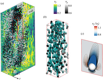


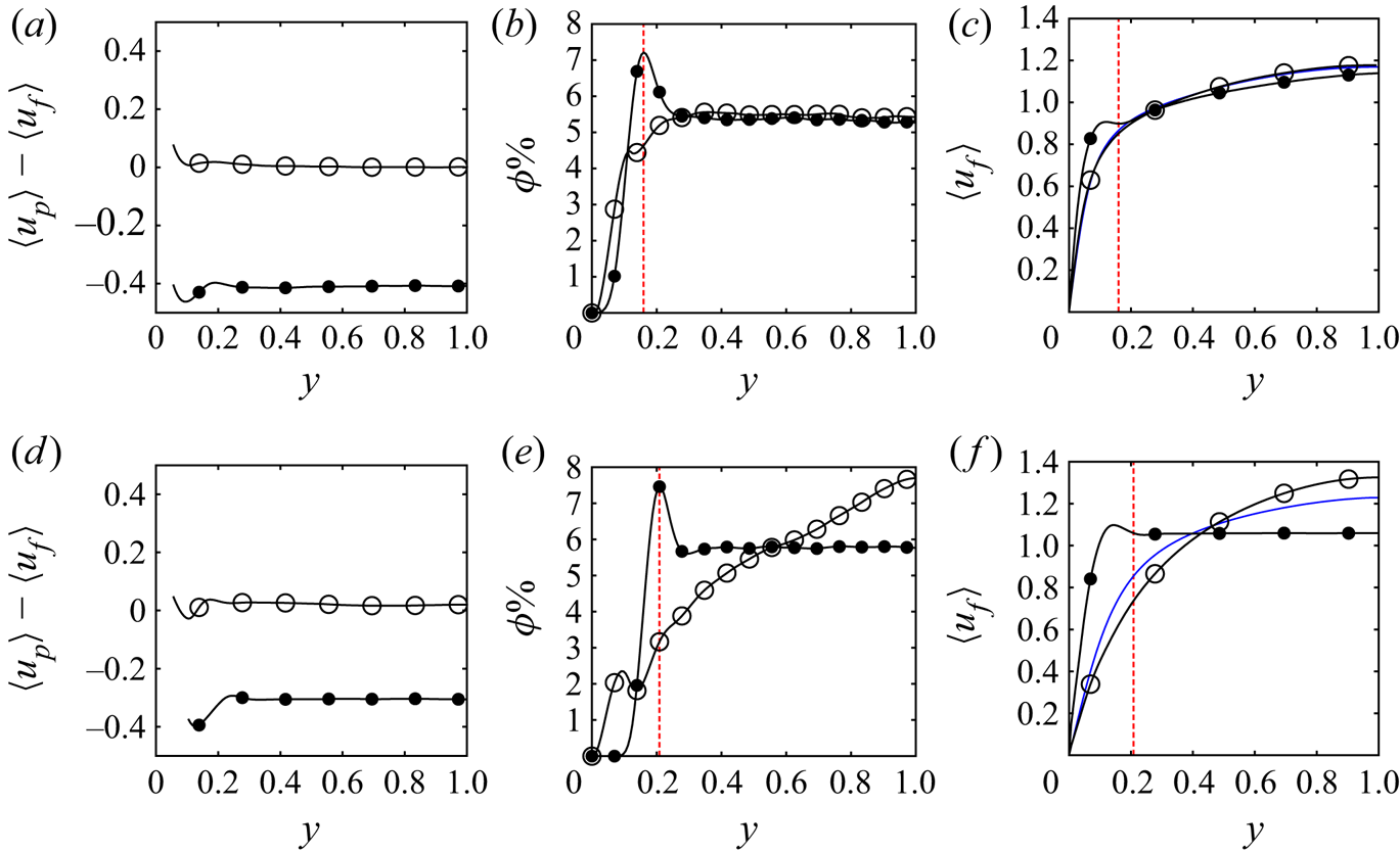
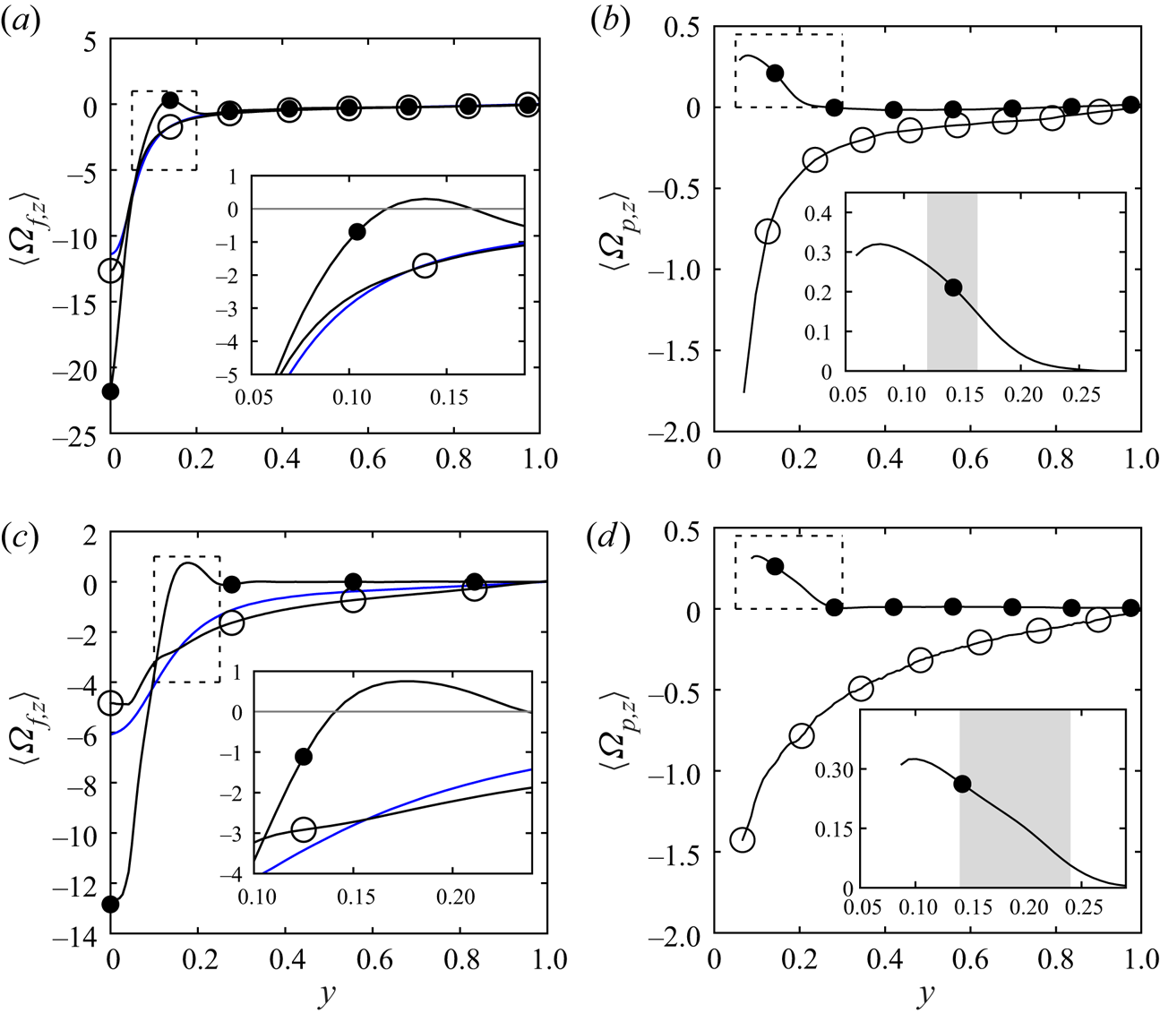


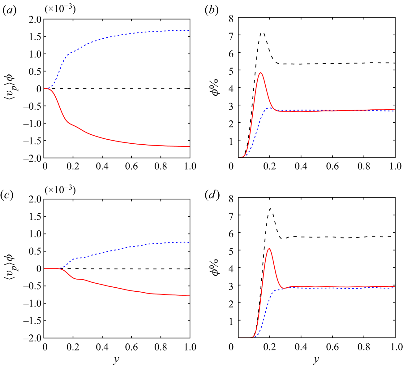


 $d_p, and the preferential transport of aggregated particles towards the wall. (



