3. Data

The NFHS is a large-scale, multi-round survey conducted among a nationally representative sample of households covering over 99% of India's population. The survey collected information on population, health, and nutrition, with a focus on women and young children, and included questions about reproductive health and family planning services (World Bank). There have been four rounds of the NFHS for the years 1992–1993, 1998–1999, 2005–2006, and 2015–2016. NFHS-1 sampled 89,777 ever-married women aged 13–49, NFHS-2 sampled 90,303 ever-married women aged 15–49, NFHS-3 sampled 124,385 ever-married women aged 15–49, and NFHS-4 sampled 699,686 women aged 15–49.Footnote 9

In each state, the rural sample was selected in two stages, with the selection of Primary Sampling Units (PSUs), which are villages, with probability proportional to population size (PPS) at the first stage, followed by the random selection of households within each PSU in the second stage. Villages with fewer than five households were omitted, and villages with fewer than 50 households were combined with other contiguous villages. In urban areas, a three-stage procedure was followed. In the first stage, wards were selected with PPS sampling. In the next stage, one census enumeration block (CEB) was randomly selected from each sample ward. In the final stage, households were randomly selected within each selected CEB. An average of 20–30 households were targeted per PSU with a target range of 15–60.

Reflecting changing geopolitical boundaries in India over time, the first survey covered 25 states, the second and third 26 states, and the fourth 29 states as well as India's six union territories. Newly created states may differ from their mother state in ways that would affect regression results, so we use the newest state and territory definitions when controlling for state fixed effects. However, results are confirmed when aggregating observations to their original state groupings (and dropping observations from the union territories which do not appear in the first three rounds of the NFHS), and are available upon request.

This study uses all four rounds of the NFHS and includes data on all women who have had at least two or three births, depending on the regression model. All descriptive statistics presented below are based on sampling-weighted estimates, since oversampling in some areas could otherwise bias outcomes. The sampling weights are the national-level weights provided by NFHS, which are appropriate when conducting analysis above the state level.

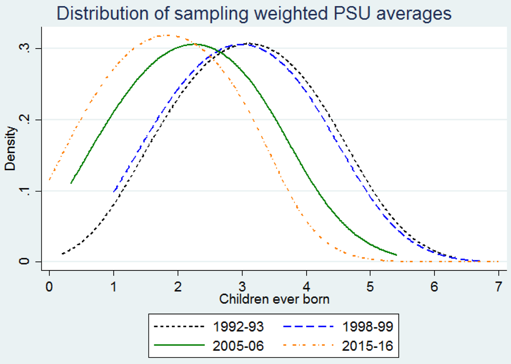
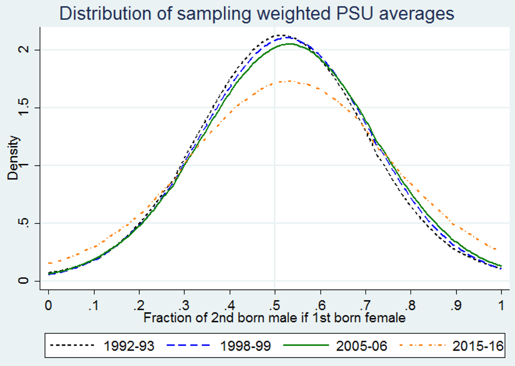
Figures 1 and 2 present the distributions of sampling-weighted PSU-level averages of key variables for each of the four survey years to demonstrate changes in mean and variance over time. All available observations are included in the graphs, not just those used in the final regression samples. In Figure 1, the average number of children born to women in the sample declines over time, reflecting falling fertility since the early 1990s, with a clear leftward shift of the distribution between the 1990s and 2000s. Figure 2 shows that among respondents with a first-born daughter, the second birth is, on average, more likely to be male. The distribution has migrated further to the right over time, coinciding with the fertility change in Figure 1 and thereby suggesting a fertility squeeze. Moreover, the distribution has widened over time, especially for the most recent sample year, indicating growing variation across PSUs in the practice of sex selection at second-order births. Similar trends can be shown for male third-order births when the first two births are female. Declining fertility accompanied by increasing proportions of male births following female births suggests a fertility squeeze effect. Parents are feeling growing pressure to sex select as they approach their desired family size.

Figure 1.

Children ever born per respondent, by survey wave, NFHS.

Note: First PSU averages are calculated, then probability sampling weights are applied when generating the density distributions. All available data are used for women of all ages 15–49.

Figure 2.

Proportion of second births male if first birth female, by survey wave, NFHS.

Note: First PSU averages are calculated, then probability sampling weights are applied when generating the density distributions. All available data are used for women of all ages 15–49.

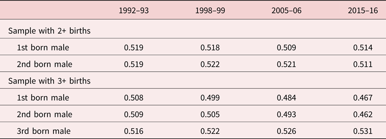
Table 1 demonstrates the average prevalence of male births by birth order for each sample year. Data are restricted to women included in the final regression samples. Among women with at least two births, more boys are born than girls at every birth order in each sample year, but there is no clear upward or downward trend over time or across births.Footnote 10 Among women with at least three births, the prevalence of male births is increasing by birth order in every sample year. In 1992, more boys than girls were born, on average, at first, second, and third births, but in 1998, there is a higher prevalence of daughters at first order, and in 2005 and 2015, a higher prevalence of daughters at first and second orders. Increasingly over time, respondents who have had at least three births tend to be those who have more daughters at earlier birth orders, with a clear reversal toward male births at the third order. This suggests an intensifying fertility squeeze whereby higher order births are pursued when the respondent has yet to yield a son.

Table 1.

Prevalence of male births by birth order, by regression sample, and by survey wave, NFHS

Note: Observations are weighted using sampling probability weights.

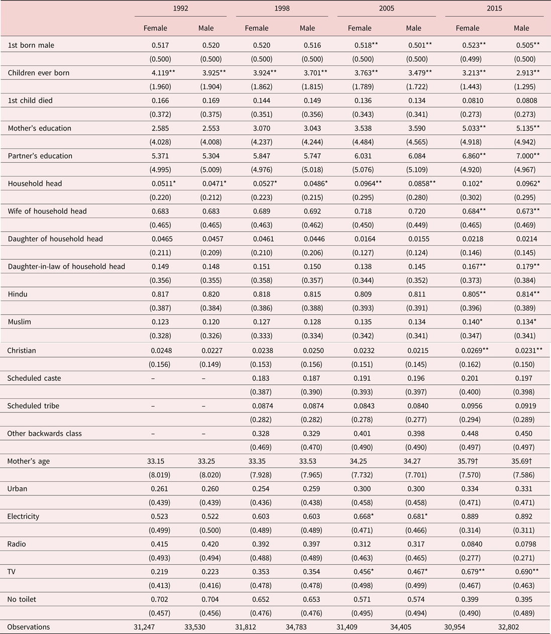
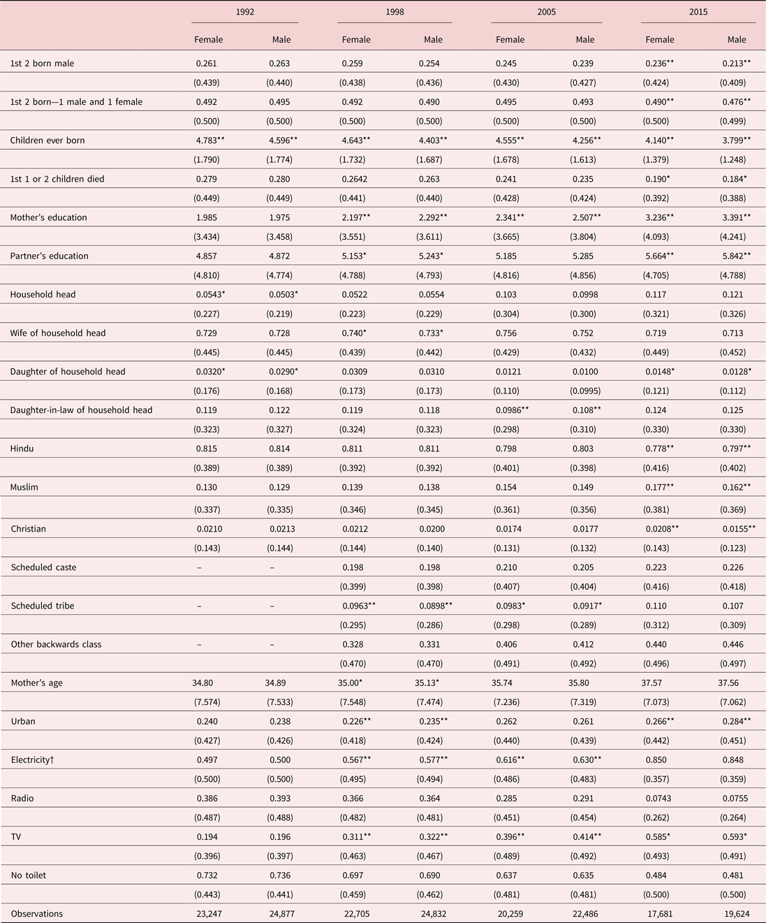
Tables 2 and 3 present the summary statistics for the samples used in the regression analysis that follows, broken down according to the sex of the respondent's second- and third-born child, respectively. The manifestation of sex selection at second births would present as a lower proportion of first-born male children among respondents who had a son at second birth compared to those who had a daughter at second birth. In 1992, the opposite is true, although the difference is statistically insignificant.Footnote ¹¹ For all following years, second-born females are more likely than second-born males to have an older brother, with the difference in means becoming statistically significant for 2005 and 2015. Regardless of year and sex of the second child, it is more common for the first child to be male, i.e., both female and male second births are more likely to have an older brother than an older sister. Fertility has clearly declined over time and is on average lower among respondents having a second-born son, suggesting that either women who successfully have a son are less likely to continue having children, or conversely that where desired family size is smaller, the pressure to produce a son is stronger. Among women who have had at least three births (Table 3), respondents with a third-order male birth have a lower prevalence of previous male births, with the exception of the 1992 sample when a fertility squeeze effect would have been weakest at this earlier stage of the demographic transition.Footnote ¹² The difference in means is not, however, statistically significant until 2015.

Table 2.

Summary statistics of a sample of second-born children by sex of the child and by survey wave, NFHS

Note: Observations are weighted using sampling probability weights. Statistically different means are indicated at the †10%, *5%, and **1% levels.

Table 3.

Summary statistics of a sample of third-born children by sex of the child and by survey wave, NFHS

Note: Observations are weighted using sampling probability weights. Statistically different means are indicated at the †10%, *5%, and **1% levels.

Previous research suggests more masculine SRBs among the more educated and wealthy in India [Madan and Breuning (Reference Madan and Breuning2014), Portner (Reference Portner2016)]. More educated women may have a higher opportunity cost of children and thus lower desired fertility, which would affect the birth order at which the pressure to sex select occurs [Clark (Reference Clark2000)]. More educated women may also be better informed about accessing sex-selective abortions [Arokiasamy (Reference Arokiasamy, Attané and Guilmoto2007), Bhat and Zavier (Reference Bhat and Zavier2003)]. On the other hand, greater education of women might be associated with the higher perceived status of women, which would weaken the preference for sons, although this does not seem to be the case in India. In Tables 2 and 3, education has increased over time, with some narrowing of the gap between men and women, but is not consistently higher or lower among families with second- or third-born male children. More homes have electricity, toilets, and a television, indicating improving living standards, while radio ownership has decreased over time. Of these, only television ownership is consistently higher in homes with a second- or third-born male, although the difference in means is statistically significant only more recently. The respondent's relationship to the head of the household includes the categories: self, wife, daughter, daughter-in-law, granddaughter, mother, mother-in-law, sister, other relative, adopted/foster child, not related, sister-in-law, niece, and domestic servant. Only statistics for the first four are presented in Tables 2 and 3. Women residing with their in-laws may face more pressure to sex select [Robitaille (Reference Robitaille2013)], although this is not apparent in the descriptive statistics. In Table 2, second-born females are more likely to have a mother that is the household head. Although Hinduism has been more strongly associated with son preference than Islam and Christianity, Tables 2 and 3 do not reflect this until 2015 when the differences in means become statistically significant [Guilmoto (Reference Guilmoto2009)]. Religious composition remains stable, with approximately 81% of the Indian population Hindu, 13% Muslim, and 2% Christian in Table 2. In Table 3, a decreasing proportion of families with at least three births are Hindu and an increasing proportion are Muslim, reflecting differences in the pace of fertility decline. The descriptive statistics thus far suggest that the sex of later births is largely conditional on the sex of previous births and is related to fertility levels [Gu and Roy (Reference Gu and Roy1995), Yang and Wang (Reference Yang and Wang2006)].

4. Empirical analysis

4.1 Methodology

The demand for sex selection may vary at different birth orders depending on desired fertility size such that a family desiring a total of two children would act on their son preference at the second birth, while a family desiring a total of three children might not do so until the third birth, in the case that the previous births were female. The following regression analysis accounts for differences in desired fertility by investigating whether the impact of sex composition of children on the sex of a subsequent birth is affected by local fertility rates. We expect the evidence of sex selection to be stronger among women living in areas with lower fertility rates [Guilmoto (Reference Guilmoto2009)]. The use of local fertility rates avoids reporting bias inherent in individually-reported ideal family size [Jayachandran (Reference Jayachandran2017)] and reflects the influence of social norms and geographically-shared socioeconomic influences on fertility [Bloom et al. (Reference Bloom, Canning, Günther and Linnemayer2008)].

We further explore unobserved geographic heterogeneity in the degree of son preference and sex selection through the use of mixed-effects models. Assuming that retrospective reporting may bias stated ideal sex ratios of children and also that survey respondents do not accurately report if they have engaged in sex selection, the data set lacks accurate information about son preference and sex selection. Mixed-effects models allow for standard random effects (different intercepts for each geographic area) but also for different effects of selected covariates. In our case, the probability of having a son based on the sex composition of previous births is allowed to differ by village or urban neighborhood. This methodology accounts for some of the potential bias inherent in the regression models.

We implement a mixed-effects logit estimation with two levels. At the first level, the indicator ${\bf {\cal S}}on_{ij}$ takes the value of one if woman i in geographic area j gave birth to a son. Otherwise ${\bf {\cal S}}on_{ij}$ takes the value of zero. Second- and third-order births are separately considered: the first set of models considers women who have had at least two births, and the second set of models includes only those women who have had at least three births, estimating the probability of a male second- or third-order birth, respectively. In the second level, we account for geographic heterogeneity by allowing some coefficients to vary across PSU. The two-level logit models are specified as follows:

(1)$$logit\lpar p_{ij}\rpar = {{X}}_{ij}\beta + Z_{ij}u_j + \varepsilon _{ij}\comma \;$$

where $p_{ij} = {\bf {\cal P}}r\lpar {\bf {\cal S}}on_{ij} = 1\rpar$ for woman i living in PSUj, X is a vector of variables potentially associated with son preference, Z is a subset of factors assumed to have heterogeneous effects across PSUs, and ɛ is the error term that follows a logistic distribution. β is the vector of relevant fixed effect coefficients to be estimated, and u _j is a set of random effects that depict heterogeneity across PSUs. The random-intercept logit model is obtained when vector Z is reduced to a vector of ones. In this model, the effects of covariates on the probability of a son being born are assumed to be fixed, but the intercept is allowed to vary across PSUs to account for heterogeneity. As an extension of this model, a subset of variables is included in vector Z to estimate a random-coefficient logit model in which the estimated effects of those variables are allowed to randomly vary across PSUs. We explore the possibility that the sex composition of previously born children can have mixed (fixed and random) effects on the probability of a son being born by including sex composition as an indicator variable in vector Z. Finally, robust standard errors are clustered by PSU.

The vector X includes variables that indirectly capture household wealth, education, and exposure to media, while maximizing sample size. Specifically, X includes the presence of electricity and a toilet in the home, education of the woman and that of her partner, and ownership of a radio or television. We control for woman's age since the reported second- or third-order births could have occurred as recently as in the past year or up to 34 years ago for any particular survey year. Death of a child is included as this could influence fertility decisions within the household. Indicator variables for the most dominant religions are also included in X, since these will reflect differences in traditions which may influence son preference. The respondent's relationship to the household head controls for family pressures in the decision to sex select. An indicator variable for urban is included, since desired family size tends to be lower in urban areas thereby affecting the rate of fertility squeeze. State fixed effects control for state-level heterogeneity in son preference not captured by the individual control variables.

While the caste system permeates Indian society, this is not explicitly included in the main regressions due to inconsistency in reporting across survey years. Many mechanisms by which caste might influence both fertility and son preference, however, are accounted for through the other control variables. Moreover, recent research by Borker et al. (Reference Borker, Eeckhout, Luke, Minz, Munshi and Swaminathan2018) demonstrates substantial variation in sex selection within castes in India, so that members of any particular caste are not homogeneously more or less likely to sex select. Nevertheless, we conduct robustness checks of all regressions by including caste for the three years available, 1998–99, 2005–06, and 2015–16.

The rate of fertility decline has differed throughout India [Das Gupta and Bhat (Reference Das Gupta and Bhat1997)]. The PSU average level of children born per respondent is included in ${\bf {\cal X}}$ as a proxy for the local fertility rate as this may affect fertility decisions at the household level. If fertility rates have declined locally, social norms may push couples to choose to have fewer children and, through the fertility squeeze, to sex select at lower order births. The regressions that follow present results with and without this PSU average number of children born per woman, as well as with the average interacted with the sex of previously born children. To make the PSU average a meaningful measure, and to avoid endogeneity at the individual respondent level, all observations in PSUs numbering less than five households are dropped from the regression analysis.Footnote ¹³ These make up an imperceptible fraction of the observations, 71 out of 260,942 for the second-order birth regression sample and 40 out of 175,711 for the third-order birth regression sample. On average, there are 31 households per PSU in the regression samples.

Unobserved heterogeneity at the PSU level could cause variation in the manifestation of son preference. Early on in the data, this may include geographic differences in access to sex-determination technology. While ultrasound technology was widespread in India by the 1990s, access did continue expanding throughout that decade [Bhalotra and Cochrane (Reference Bhalotra and Cochrane2010)]. Unfortunately, data collection on ultrasound usage is only available for a small subset of the sample and not at all for 1992–93, so it is not included in our regression models. We discuss the implications later in Section 4.2. However, PSU-level random effects (u _j in equation 1) can account for some of this unobserved heterogeneity in access to sex-determination technology.

There remains potential heterogeneity in social norms affecting the degree of son preference or at least the willingness to sex select. The preference for sons may itself differ across states or more locally between villages or throughout major urban areas depending on economic and educational opportunities for women, religious traditions, and other social norms. While the control variables in X aim to account for such variation, they cannot capture all social norms or even wealth effects completely, so there may remain unobserved heterogeneity. Moreover, even for a particular degree of son preference, social norms may affect how individuals act upon that son preference, whether it manifests in sex-selective abortions, or even infanticide, or whether parents use the more natural “stopping rule”, having children until the desired number of sons is born. Since responses to survey questions regarding sex selection cannot be considered reliable, in part due to the illegality of both sex-selective abortions and of infanticide, individual-level preferences cannot be directly measured [Arnold et al. (Reference Arnold, Kishor and Roy2002)]. Assuming social norms play a role in son preference and the proclivity to actually sex select, PSU-level random effects can account for some of this potential bias by controlling for unobserved community-level heterogeneity.

Sex selection at earlier births may affect the tendency to sex select at higher order births. If those having a third birth sex selected at previous births, they might be more likely to sex select again but to also have more sons, thereby biasing our results toward a weaker effect of having sons on the probability of having another son. If those having a third birth have not sex selected at previous births, they may be less willing and therefore less likely to sex select at the third order but also have more daughters, similarly biasing the estimated effects downward. Once again assuming social norms play a role in son preference and the proclivity to actually sex select, PSU-level random effects can account for some of this potential bias.

There could also be some sex selection occurring at first-order births, although past evidence concludes this an uncommon practice and is much more likely at higher order births [Ebenstein (Reference Ebenstein2007), Portner (2016), Jha et al. (2011), Rosenblum (Reference Rosenblum2013)].Footnote ¹⁴ However, to the extent that sex selection is occurring at the first order, this would bias the regression results that follow, which assume that the sex of the first-born child is exogenous, i.e., not affected by son preference. Again, PSU-level random effects can account for some of this potential bias. Moreover, analysis by Bhalotra and Cochrane (Reference Bhalotra and Cochrane2010) concludes that unobserved mother-level heterogeneity in sex selection is not statistically significant in India.

4.2 Regression results

4.2.1 Sex selection at second-order births

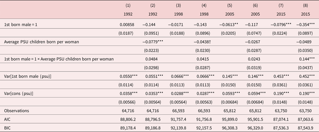
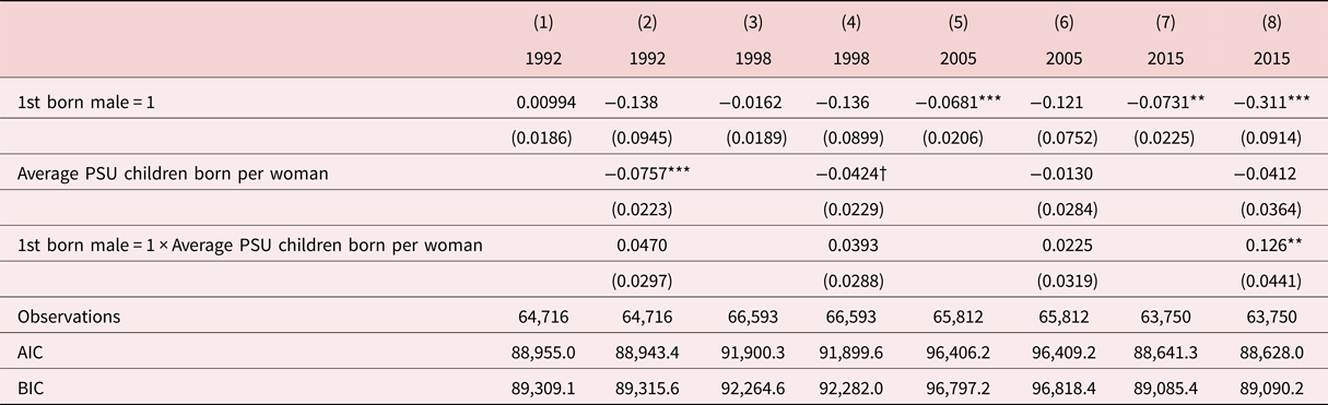
Table 4 presents the results regressing probability that the second-born child is male on the sex of the first-born child and all of the control variables (not shown) for each sample year. Observations are weighted using sampling probability weights in these and all regressions that follow. If son preference is present and is manifesting in sex selection, then we expect a negative coefficient on the explanatory variable of interest, a first-born son. For each year, two models are presented: with and without average PSU children born per woman and its interaction with the sex of the first-born child. The latter investigates geographic variation in the fertility squeeze, that is, potentially more sex selection at lower order births where smaller families are the norm. Later, comparison with the regressions of third-order births will provide additional insight into the progression of the fertility squeeze over time. Coefficient estimates and statistical significance are similar across the logit, random-intercept, and random-coefficient models, but likelihood ratio tests favor the random-coefficient model over the basic logit and the random-intercept models in each case. Thus, only the random-coefficient estimates are discussed in the interest of brevity. The logit regression results are available in the Appendix.

Table 4.

Random coefficients regressions: second-born male

Observations are weighted using sampling probability weights. All regressions include state fixed effects and control variables. Clustered standard errors in parentheses.

†p < 0.10,

*p < 0.05,

**p < 0.01,

***p < 0.001.

Comparing results across years demonstrates little evidence of sex selection at second-order births in 1992 and 1998 but clear evidence in 2005 and 2015; where the first-born child is male, the likelihood is lower that the second-born will also be male, relative to the benchmark of a first-born daughter. The 2015 results indicate variation in the fertility squeeze across PSUs; where fertility is lower, there is an even lower probability that a first-born son is followed by the birth of another son. Notably, few of the control variables are statistically significant. Partner's education is associated with a lower probability of a son at second parity, but the results are not significant across all years. Respondents who live with their in-laws are more likely to sex select, although this too is not consistent across years. Respondents who live with their children (i.e., those reporting they are the mother of the household head) are more likely to sex select, suggesting that more traditional living arrangements whereby parents live with their married son are associated with sex selection. Generally, though, it seems that sex of the first-born child is the key predictor of whether a second-born child will be male, with stronger effects where the fertility transition is more advanced.

The magnitude of the random-coefficient estimates is sizable (0.15 in 2005 and 0.45 in 2015) relative to the estimated β coefficients. Unobserved heterogeneity at the PSU level is causing substantial variation in the manifestation of son preference at second-order births, even after controlling for PSU heterogeneity in fertility rates.

4.2.2 Sex selection at third-order births

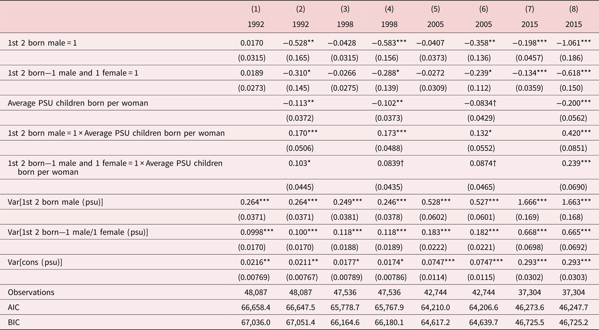
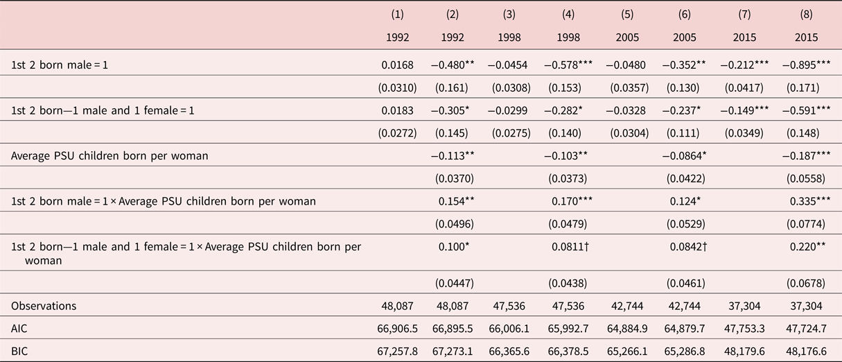
The lack of evidence of sex selection for earlier years is likely due to the pace of demographic transition. India's TFR was approximately 3.8 in 1992–93, 3.4 in 1998–99, 2.9 in 2005–06, and 2.3 in 2015 (World Bank Indicators). With a higher fertility rate, the pressure to sex select may not manifest until higher order births. Table 5 presents the results regressing the probability of a third-born male birth on sex composition of the first- and second-born children. Again, if son preference is present and manifesting in sex selection, we expect a lower probability of the third-born child being male if at least one son is already born, and even more so if there are already two sons, relative to the benchmark of two previous female births. This effect is likely stronger where fertility rates are lower as families act to fulfill the dual desires of having sons but also a small family. Again, we present only the random-coefficient estimates as these are supported by likelihood ratio tests over the basic logit and the random-intercept models.

Table 5.

Random coefficients regressions: third-born male

Observations are weighted using sampling probability weights. All regressions include state fixed effects and control variables. Clustered standard errors in parentheses.

†p < 0.10,

*p < 0.05,

**p < 0.01,

***p < 0.001.

Unlike the regressions of second-order births, we see evidence of sex selection at the third-order birth even as early as 1992 once we account for variation in fertility rates. That is, the fertility squeeze was affecting third-order births at least as early as 1992, but not yet second-order births. The direct effect of having two sons is stronger than that of having one son and one daughter.Footnote ¹⁵ Geographic heterogeneity strengthens over time as reflected by increasing magnitudes of the random-coefficient estimates (0.26 and 0.10 in 1992 up to 1.66 and 0.67 in 2015). As with the second-order birth regressions, this magnitude relative to the β coefficient estimates on sex composition indicates the importance of the unobserved, community-level heterogeneity. Again, few of the control variables are statistically significant. Respondent's education and living with one's children are associated with a higher probability of a son at third parity, but these are significant only for some years.

4.3 Robustness checks

We further examine the results at second- and third-order births by disaggregating the samples by rural–urban, regionally, and by respondent's age.

4.3.1 Urban–rural

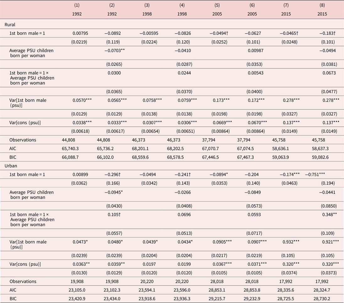
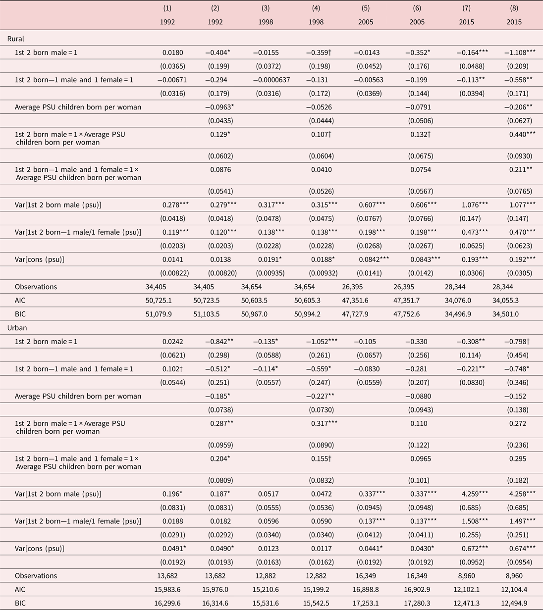
Tables 6 and 7 segment the sample into respondents residing in rural vs urban areas. At second-order births (Table 6), there is weaker evidence of sex selection in urban areas in the 1990s that strengthens in statistical significance into the 2000s. For rural areas, sex selection at second-order births appears only in the 2000s. Evidence of geographic variation in the fertility squeeze is apparent only in the urban sub-sample. In other words, urban trends are the primary driver of the main results in Table 4. At third-order births (Table 7), there is evidence of sex selection as early as 1992 in both rural and urban areas, as in the main results in Table 5. Moreover, evidence of sex selection and variation in the fertility squeeze appear stronger in rural areas most recently and in urban areas in the 1990s. Comparing Tables 6 and 7, most recently, variation in the fertility squeeze emerges in urban areas at second-order births and strengthens in rural areas at third-order births, consistent with lower desired fertility in urban areas. Increasing magnitudes of the random-coefficient estimates also indicate growing heterogeneity in sex selection in both rural and urban areas.

Table 6.

Random coefficients regressions: second-born male—rural vs urban

Observations are weighted using sampling probability weights. All regressions include state fixed effects and control variables. Clustered standard errors in parentheses.

†p < 0.10,

*p < 0.05,

**p < 0.01,

***p < 0.001.

Table 7.

Random coefficients regressions: third-born child male—rural vs urban

Observations are weighted using sampling probability weights. All regressions include state fixed effects and control variables. Clustered standard errors in parentheses. †p < 0.10, *p < 0.05, **p < 0.01, ***p < 0.001.

4.3.2 By region

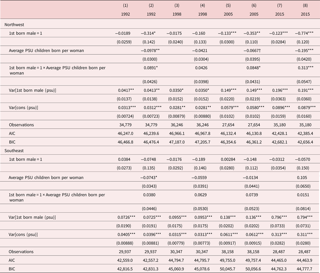
Geographic variation at the larger regional level is more closely investigated in Tables 8 and 9. Dyson and Moore (Reference Dyson and Moore1983) demonstrated that a northwest–southeast divide exists in India regarding sex ratios and other demographic variables such as mortality and fertility, which is approximated by the contours of the Satpura hill range extending from the Gujarat–Maharashtra border on the west coast up to southern Bihar in the east where it joins the Chota Nagpur hills. States north of this demarcation have historically exhibited more masculine sex ratios than states south of the line, even pre-dating the spread of ultrasound technology. Accordingly, we now apply this classification by grouping observations into states falling in the regions “Northwest” and “Southeast”.Footnote ¹⁶

Table 8.

Random coefficients regressions: second-born male—by region

Observations are weighted using sampling probability weights. All regressions include state fixed effects and control variables. Clustered standard errors in parentheses.

†p < 0.10,

*p < 0.05,

**p < 0.01,

***p < 0.001.

Table 9.

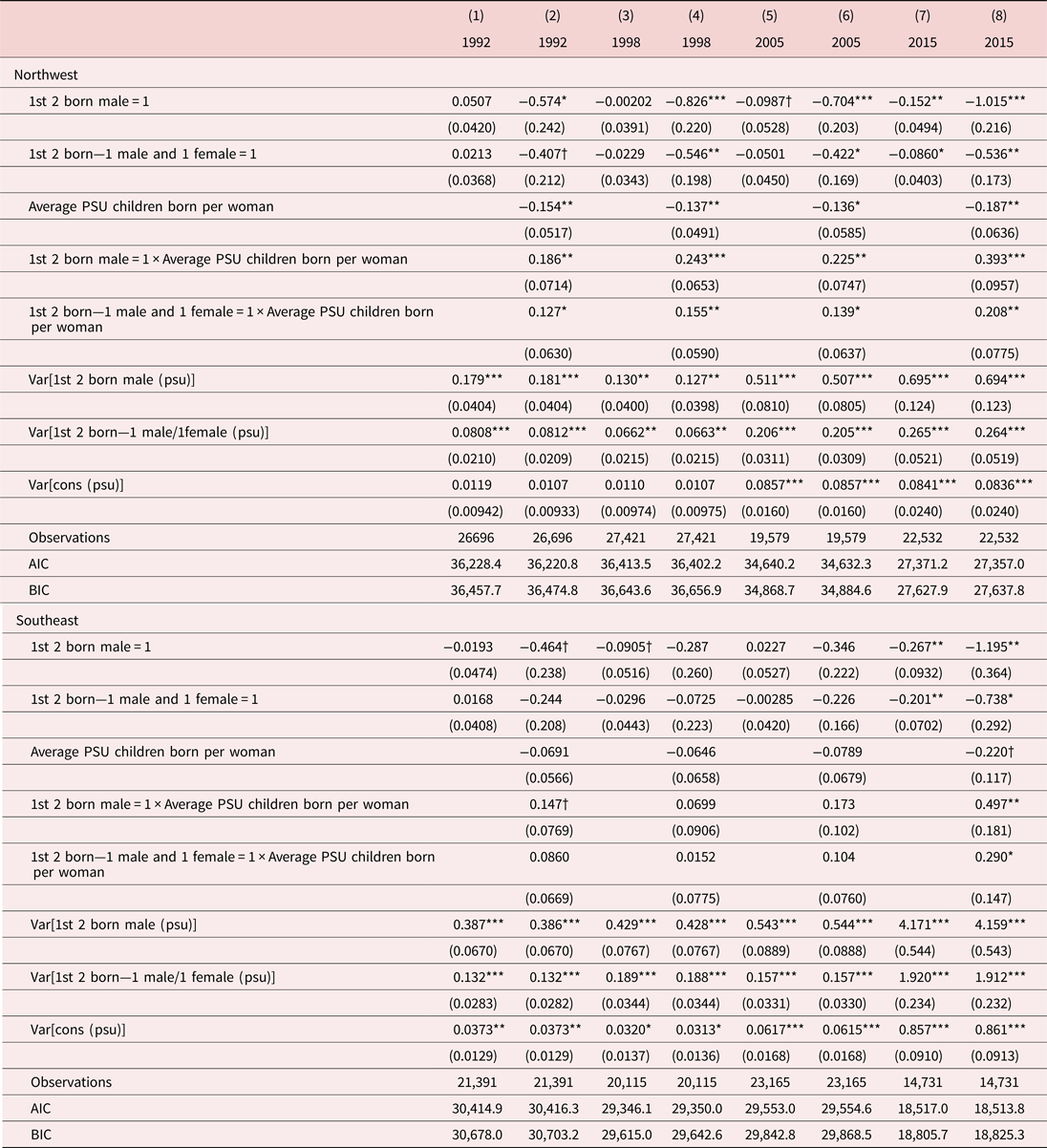
Random coefficients regressions: third-born male—by region

Observations are weighted using sampling probability weights. All regressions include state fixed effects and control variables. Clustered standard errors in parentheses.

†p < 0.10,

*p < 0.05,

**p < 0.01,

***p < 0.001.

Table 8 indicates that the results for second-order births in Table 4 are being driven by the Northwest, such that sex selection appears to be occurring in the Northwest as early as 1992, and certainly in the 2000s, but not in the rest of the country. PSU-level heterogeneity is significant and generally growing over time in both regions but especially in the Southeast. Table 9 indicates that the results for third-order births in Table 5 are also being driven primarily by the Northwest until most recently, but by 2015, evidence of sex selection emerges in the Southeast also. The fertility squeeze is finally affecting even this region of the country where sex ratios have traditionally remained more balanced. Again, PSU-level heterogeneity is growing over time in both regions, and the random-coefficient estimates are particularly large for the Southeast.

4.3.3 By respondent age

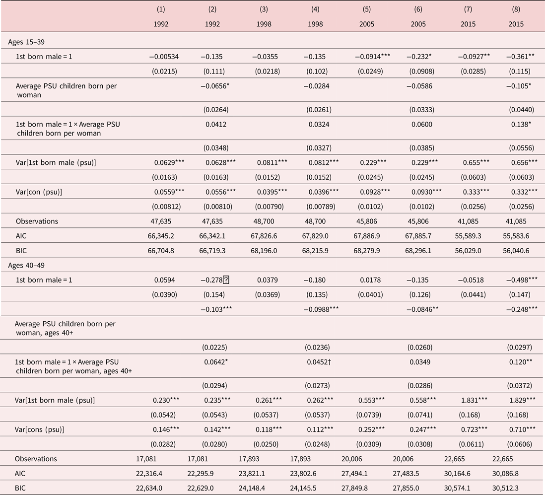
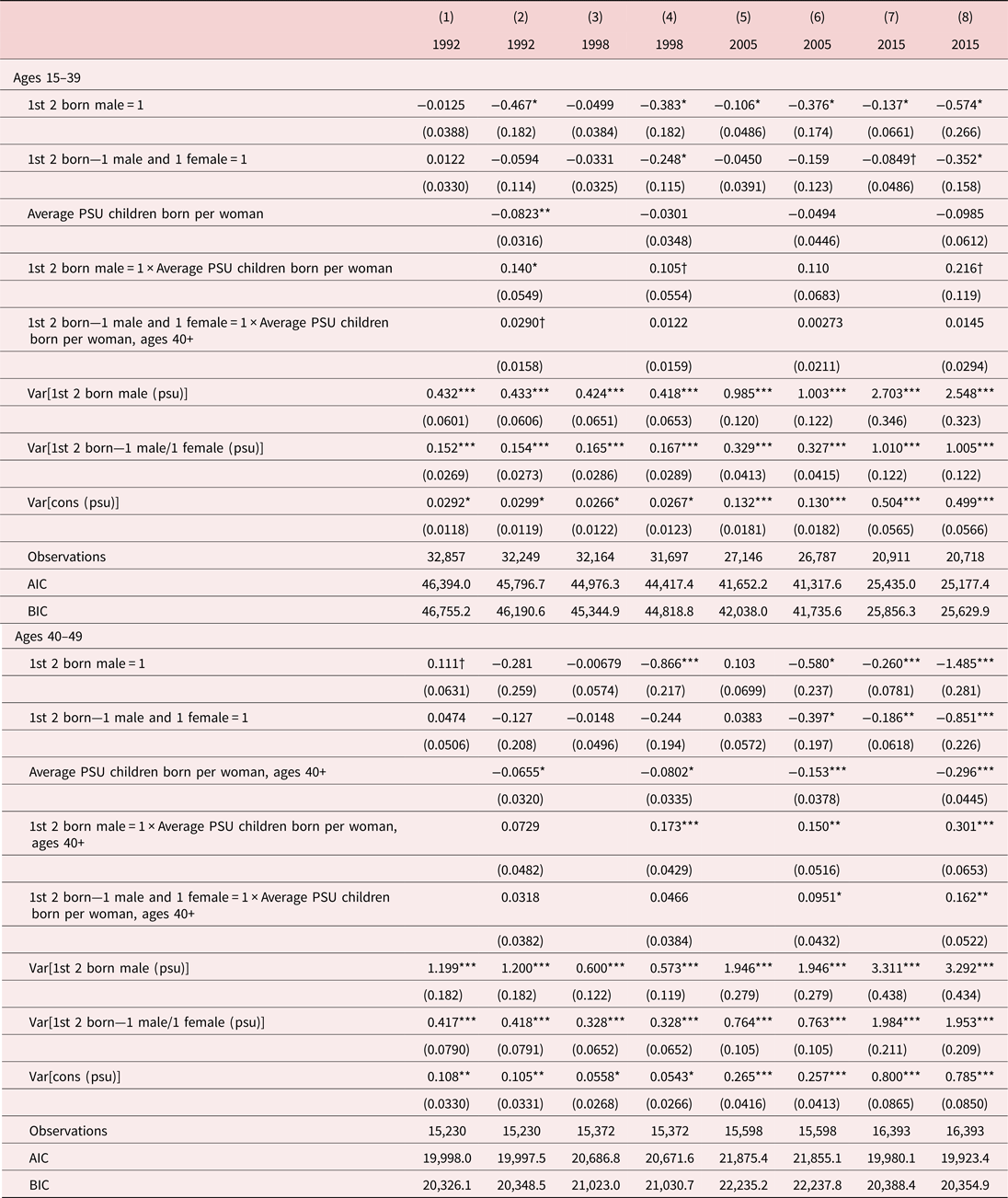
The regressions pool women at various stages of fertility, which may mask changing social norms. Second- or third-order births of older women could appear in numerous regression years. Tables 10 and 11 segment the sample into respondents less than 40 years old and those 40 and older to investigate whether sex selection is indeed occurring recently or whether the results in Tables 4 and 5 are being driven by remnants of sex-selective practices of older cohorts whose fertility is for the most part completed. Results are similar for small variations in the age groupings. For the older cohort, the PSU average number of children born to respondents is re-calculated to include only the birth histories of women 40 years and older; the fertility behavior of younger women would not have affected past fertility choices of older women, although underlying trends impacting the fertility of younger women would evolve over a longer time frame. Consistent with the main results in Tables 4 and 5, there is evidence of sex selection at second-order births in the 2000s (Table 10) and at least some at third-order births as early as 1992 (Table 11) across younger and older women. Most recently, in 2015, there is variation in the fertility squeeze among both age groups for both second- and third-order births (column 8). Among the older women, these births likely occurred several years in the past and therefore represent the fertility squeeze with some lag. Weaker statistical significance among younger women in column 8 of Table 11 suggests that variation in fertility norms has less effect at third-order births now that India's TFR is below 3. Taken together, Tables 10 and 11 demonstrate sex selection among women earlier in their childbearing years up until most recently, confirming that the practice is not a fading phenomenon.

Table 10.

Random coefficients regressions: second-born male—by age group

Observations are weighted using sampling probability weights. All regressions include state fixed effects and control variables. Clustered standard errors in parentheses.

†p < 0.10,

*p < 0.05,

**p < 0.01,

***p < 0.001.

Table 11.

Random coefficients regressions: third-born male—by age group

Observations are weighted using sampling probability weights. All regressions include state fixed effects and control variables. Clustered standard errors in parentheses.

†p < 0.10,

*p < 0.05,

**p < 0.01,

***p < 0.001.

4.3.4 Caste

As a robustness check, all of the above regressions are repeated controlling for caste. Specifically, the NFHS identifies each respondent by whether she belongs to a scheduled caste (19–22%), scheduled tribe (9–10%), or other backwards class (33–45%). The 1992–93 regressions are omitted because of lack of data for this variable. Regression results are not importantly altered by this addition and are available upon request.

4.3.5 Ultrasound access

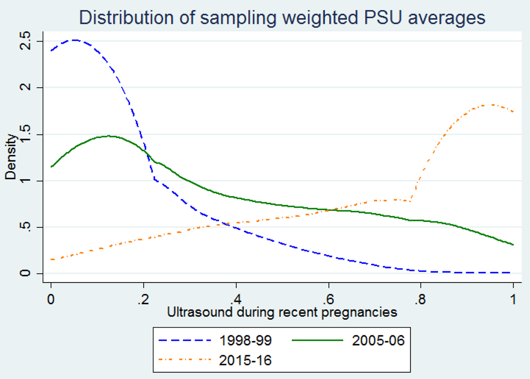
Because of data limitations, none of the regression results presented account for access to sex-determination technology, and this could be driving some of the outcomes. As the access to ultrasound technology spread, so would evidence of sex selection, as in Table 4 where sex selection at second-order births shows up only more recently in the 2000s. However, evidence of sex selection at third-order births as early as 1992 (Table 5) suggests that access to technology is not driving these results. Variation in access to sex-determination technology might also explain the PSU-level heterogeneity indicated by the random-coefficient estimates. Figure 3 illustrates the rising prevalence of ultrasound usage over time. Variation increased between 1998 and 2005 and then decreased again by 2015 as the distribution shifted strongly to the right. Thus, it is unlikely that variation in ultrasound usage explains the strong, monotonic increase in unobserved heterogeneity indicated by the mixed-effects regression results. Nevertheless, data limitations make it difficult to properly assess the role of technology diffusion in driving the heterogeneity results.

Figure 3.

Proportion of respondents reporting at least one ultrasound, conditional on having been pregnant within the past 5 years, by survey wave, NFHS.

Note: First PSU averages are calculated, then probability sampling weights are applied when generating the density distributions. All available observations are included in the graphs, not just those used in the regression samples. The sample sizes here are: 39,156 for 1998–99, 206,048 for 2005–06, and 190,959 for 2015–16.

5. Conclusion

The tendency for son preference to decline with economic development may alleviate concerns about India's masculinized SRB [Bongaarts (Reference Bongaarts2013)]. Yet falling desired family size can have the perverse effect of intensifying these imbalances, even as actual son preference weakens, by pressuring parents to sex select at earlier parities. Indeed, the analysis presented here demonstrates sex selection at increasingly earlier parities, consistent with the “intensification effect” described by Das Gupta and Bhat (Reference Das Gupta and Bhat1997).

This paper is the first to combine all four waves of India's NFHS to examine the influence of the fertility transition on the country's notoriously skewed SRB. The regression results demonstrate a fertility squeeze at third-order births in even the earliest survey years (1992–93), while the effect at second-order births does not emerge until more recently, beginning with the 2005–06 survey and strengthening for 2015–16. Accordingly, India's TFR fell from 3.8 to 2.35 during this time [World Bank Indicators (2015)]. The analysis also accounts for unobserved heterogeneity at the village or urban neighborhood level that may affect the degree of son preference and its propensity to manifest in sex selection. Unlike Bhalotra and Cochrane (Reference Bhalotra and Cochrane2010) who conclude that heterogeneity at the individual mother level is of little importance in India, we show that heterogeneity at the community level is considerable in magnitude and has increased over time, even after controlling for geographic variation in the pace of fertility decline. Future research may determine the drivers of this heterogeneity, whether they are access to health care facilities willing to provide abortions or specific cultural or socioeconomic factors not captured in the estimated models. Without explicitly controlling for ultrasound access, it is unclear to what degree technology access is driving the unobserved heterogeneity. Having controlled for desired fertility, we find no systematic impact of religion, caste, household structure, exposure to media, or education or wealth levels on the propensity to sex select in the regression analysis here, supporting Basu's argument of cultural convergence throughout India as lower socioeconomic groups imitate upper ones, which tend to have both stronger son preference and lower fertility [Basu (Reference Basu1999)].Footnote ¹⁷ Future research may further examine cultural and socioeconomic factors by including more refined measures of caste, access to sex determination technology, and economic status.

As it has become easier for parents to control the sex composition of their children, the health and education outcomes of the so-called “wanted” daughters have been found to improve [Mishra et al. (Reference Mishra, Roy and Retherford2004), Chamarbagwala (Reference Chamarbagwala2011), Hu and Schlosser (Reference Hu and Schlosser2012), Rosenblum (Reference Rosenblum2013), Hazan and Zoabi (Reference Hazan and Zoabi2015)], making sex-selective abortion a mechanism by which discrimination against girls is being replaced by discrimination against female fetuses [Anukriti et al. (Reference Anukriti, Bhalotra and Tam2018)]. Conditional cash transfer programs that subsidize daughters have met with mixed success and are, of course, subject to funding availability [Anukriti (Reference Anukriti2018)]. Future research can pinpoint specific villages and neighborhoods that are more prone to the practice of sex-selective abortion. It is possible that social network effects play a role in the local geographic heterogeneity identified by the regression analysis here. In that case, policies may be able to exploit these social network effects to better target those couples most likely to sex select.

As desired fertility continues to decline, even decreased rates of sex selection could exacerbate sex ratio imbalances because the number of missing girls weighs disproportionately on the SRB of a small birth cohort. Accordingly, our results demonstrate sex selection at increasingly lower order births. India's SRB could eventually re-balance, as was the case in South Korea, although likely not until well after fertility rates have stabilized and further economic development counters the fertility squeeze effect. On the other hand, India may be on a path of regional convergence toward a permanently skewed SRB if the willingness to sex select persists at very low fertility [Basu (Reference Basu1999), Diamond-Smith and Bishai (Reference Diamond-Smith and Bishai2015), Rajan et al. (Reference Rajan, Srinivasan and Bedi2017)]. Our results confirm the Northwest is driving much of the aggregate trends in sex selection. But they also reveal evidence of sex selection most recently, in 2015, at third-order births in the Southeast where sex ratios have historically remained more balanced, validating anecdotal evidence of widespread discrimination against baby girls throughout the South [Madan and Breuning (Reference Madan and Breuning2014)]. The increase in unobserved heterogeneity in sex selection is also particularly strong for the Southeast. This might reflect a cultural shift in that region, but it could also be indicative of a different threshold for the fertility squeeze, with underlying son preference only recently manifesting is skewed sex ratios in this region. Kashyap and Villavicencio (Reference Kashyap and Villavicencio2016) describe the preconditions for couples to sex select as RWA, or ready (fertility squeeze), willing (son preference), and able (technology). Couples may have long been “willing” to sex select but have only recently been “ready” to do so as desired family size falls further. With fertility falling, sex selection occurring at increasingly earlier parities, and sex selection emerging outside the Northwest, India's SRB is poised to continue rising in the coming years.