2.1 Production patterns of cross-word nasal place assimilation

Most of the research on the production of cross-word nasal place assimilation has focused on whether assimilation is complete or incomplete, and evidence has been found for both possibilities. In terms of acoustic measures, for instance, Gow (Reference Gow2001) finds evidence that the assimilation can be incomplete, while Zimmerer et al. (Reference Zimmerer, Reetz and Lahiri2009) and Dilley & Pitt (Reference Dilley and Pitt2007) report evidence of acoustically complete assimilation. Similarly, there is also articulatory evidence for both incomplete (e.g. Barry Reference Barry1985, Kerswill Reference Kerswill1985, Ellis & Hardcastle Reference Ellis and Hardcastle2002) and complete (Ellis & Hardcastle Reference Ellis and Hardcastle2002) assimilation.

In languages that have non-optional nasal place assimilation processes, /n/ assimilates either in both pre-labial and pre-velar contexts, or only in pre-velar context – no language has only pre-labial nasal place assimilation (de Lacy Reference de Lacy2002: 194, 375–381). The source of the velar assimilation preference is most likely to be found in perception. Various discrimination studies have found that [n] and [ŋ] are more confusable than [n] and [m] (e.g. Wang & Bilger Reference Wang and Bilger1973: 1254). If place assimilation of /n/ originates in the misperception of [n] (Ohala Reference Ohala, Kingston and Beckman1990), it can be expected that /n/ will assimilate more in contexts where the result will be more confusable with [n]. This same velar preference is also observed in variable nasal place assimilation, with higher assimilation rates observed in pre-velar than pre-labial contexts. For German, Zimmerer et al. (2009: Tables II & III), for instance, report pre-velar assimilation rates of 21.5% and pre-labial assimilation rates of only 13%. Dilley & Pitt (Reference Dilley and Pitt2007) investigate the assimilation of word-final /n/ in American English in the Buckeye corpus (Pitt et al. Reference Pitt, Dilley, Johnson, Kieling, Raymond, Hume and Fosler-Lussier2007). Although they do not report assimilation separately for pre-labial and pre-velar contexts, Laura Dilley (personal communication) confirms that pre-velar contexts had higher assimilation rates (21.8% vs. 18.5%).

In addition to being influenced by grammatical factors such as place of assimilation, nasal place assimilation is also influenced by non-grammatical factors such as speech rate. Kerswill (Reference Kerswill1985) and Barry (Reference Barry1985) both investigated cross-word place assimilation in English using electropalatography, and found higher rates of assimilation at faster than slower speech rates. Kerswill reports for one speaker an assimilation rate of 50% when speaking at a normal rate, and 90% when speaking at a fast rate (1985: 31).

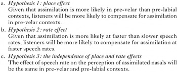
On the assumption that perception will reflect the patterns observed in production, two hypotheses can be formulated about how listeners will compensate for nasal place assimilation. Based on the assumed independence between grammatical and non-grammatical factors (see §1), a third hypothesis can be added. All three of these hypotheses are confirmed in the experiments presented in §3.

1. (1)

   

2.2 Perception of cross-word place assimilated nasals

Most of the research on the perception of nasal place assimilation has focused not on how listeners compensate for place-assimilated nasals, but rather on the likelihood that listeners would misperceive alveolar nasals as labial/velar when followed by a labial/velar consonant (i.e. that listeners would perceive an utterance like […nb…] as /…mb…/) (e.g. Ohala Reference Ohala, Kingston and Beckman1990, Hura et al. Reference Hura, Lindblom and Diehl1992, Beddor & Evans-Romaine Reference Beddor and Evans-Romaine1995). Though relevant to understanding how processes of place assimilation originates, this research is less relevant to the experiments discussed in §3, since these experiments present listeners with assimilated nasals and ask how listeners compensate for this assimilation.

There is a body of literature that shows that listeners do compensate for nasal place assimilation during perception. These results are based on experimental paradigms as diverse as word identification (e.g. asking listeners whether a phrase like [klim pæn] contains the word clean; Darcy et al. Reference Darcy, Ramus, Cristophe, Kinzler, Dupoux, Kügler, Féry and van de Vijver2009), phoneme identification (asking listeners to identify a consonant ambiguous between [m] and [n] in a phrase like lea[m/n] bacon; Gaskel & Marslen-Wilson Reference Gaskel and Marslen-Wilson1998) and priming (asking whether an assimilated nasal word primes its unassimilated citation form – i.e. does lea[m] in lea[m] bacon prime lean?; Gaskel & Marslen-Wilson Reference Gaskel and Marslen-Wilson1996, Reference Gaskel and Marslen-Wilson2001, Gow & McMurray Reference Gow, McMurray, Cole and Hualde2007). Although the details differ between these various studies, all of them find evidence that listeners do compensate for appropriately produced nasal place assimilation – that is listeners are more likely to identify a token like te[m] as an utterance of ten in a pre-labial context (te[m] pens) than in a pre-velar (te[m] cars) or pre-alveolar (te[m] toes) context. Given results such as these, we can expect to find evidence of compensation for assimilation in the experiments reported below.

Hypothesis 2 states that more compensation for assimilation is expected at faster than slower speech rates. There is also evidence that listeners do adjust their perceptual strategies based on speech rate. Most of this research focuses on the differentiation between segments that contrast in the temporal domain. Nooteboom (Reference Nooteboom, Myers, Laver and Anderson1981: 144), for instance, shows that the decision boundary between short /a/ and long /aː/ in Dutch depends on speech rate. Similar results have been reported for the distinction between short-lag and long-lag VOT plosives in English (Port Reference Port1977), the distinction between geminate and singleton consonants in Japanese (Sonu et al. Reference Sonu, Arai, Tajima and Kato2013), etc.

More directly relevant to the current paper is research showing listeners to be sensitive to the influence of speech rate on the application of phonological processes. Function words in English are subject to variable realisation at different speech rates. In slow speech, the or in a phrase like leisure or time is usually realised, while it can be completely absent at faster rates. Dilley & Pitt (Reference Dilley and Pitt2010) show that listeners are sensitive to this correlation between speech rate and the realisation of function words. Specifically, listeners are more likely to perceive the function word or at faster than slower speech rates. An eye-tracking study by Li & Kaiser (Reference Li and Kaiser2012) report similar results for cross-word nasal place assimilation in English. They first taught the participants in their study to associate the made-up names Vone ~ Vome, Kine ~ Kime and Shoon ~ Shoom with images of six imaginary creatures. They then presented their participants with sentences containing one of these six names; their task was to look at the image corresponding to the name. In the crucial sentences, these names were followed by labial-initial words – i.e. contexts in which the alveolar nasals in Vone, Kine and Shoon could assimilate to the following labial. For instance, the names were presented in sentences like Every time the waiter brings out a strawberry cheesecake from the kitchen, Vome peeks to see if he can steal a piece. They varied the speech rate of the context (the non-underlined part of the sentence), and found that listeners were significantly more likely to look at the image corresponding to the alveolar-final names (Vone, Kine, Shoon) at faster than at slower speech rates. This shows that their listeners were more likely to assume the speaker intended a final alveolar nasal, but assimilated in place to the following labial at faster speech rates. Results such as these show that listeners are sensitive to the correlation between speech rate and the application of phonological processes, adding additional support to Hypothesis 2.

The Li & Kaiser and Dilley & Pitt studies manipulated speech rate of a whole frame sentence, giving listeners a large sample of speech over which to calculate speech rate. What remains unknown is whether listeners require this much evidence to compensate for speech rate. Would their results have been the same if they had not embedded the crucial parts of their stimuli in a frame sentence, but rather presented just the crucial part at different speech rates? In the experiments reported in §3 below, the tokens were presented in isolation (not embedded in larger sentence frames), so that this question could be answered.

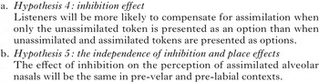
There are several ways in which listeners’ performance can be influenced by the task they are asked to carry out. Gerrits & Schouten (Reference Gerrits and Schouten2004; see also Pitt & Samuel Reference Pitt and Samuel1993), for instance, review how the results of phoneme-identification experiments can differ based solely on the format of the task that listeners have to perform (two-alternative forced choice, ABX discrimination, same–different, etc.). Different kinds of tasks place more or fewer demands on short-term memory, tap into prelexical or lexical processing, prime or inhibit competitors, etc., and all of these impact how listeners perform. In the experiments reported below, the same stimuli were presented in two different task conditions. Both experiments presented listeners with /n/-final words followed by words that start with plosives at different places of articulation. The /n/-final words were produced with place assimilation to the following plosives (e.g. te[m] pens). In Experiment 1, listeners were asked whether the stimulus contained a production of the relevant English word (i.e. ten). In Experiment 2, listeners were asked to choose from among the three possible pronunciations of the /n/-final word (te[n] ~ te[m] ~ te[ŋ]). In Experiment 1, a high percentage of ‘yes’ responses was expected. Listeners were not explicitly made aware of the possibility of the assimilated pronunciations, and would therefore not go into the task considering these pronunciations as hypotheses. In Experiment 2, however, the alternatives were presented explicitly as possible answers, and listeners would therefore approach the task with these possibilities as active hypotheses. A lower percentage of alveolar (ten) responses was expected in Experiment 2 than the percentage of ‘yes’ responses in Experiment 1. By making listeners aware of the assimilated pronunciations, these percepts were primed as hypotheses, which were therefore expected to inhibit the unassimilated, alveolar percept. This leads to a fourth hypothesis, given in (2). The assumed independence of grammatical and non-grammatical effects gives the fifth hypothesis.

1. (2)

   

A note is in order about how the experiments relate to listeners perceptual experiences in real life outside of the laboratory. Listeners are likely to be confronted with speech at different rates, so that it is easy to see why the hypothesis with regard to speech rate is relevant to everyday communicative contexts. However, listeners are rarely placed in a context such as that in Experiment 2, where they have to choose between different pronunciations of the same word. There are, however, instances in which the communicative circumstances require listeners to pay careful attention to the fine acoustic details of an utterance – this is what Lindblom et al. (Reference Lindblom, Guion, Hura, Moon and Willerman1995) call ‘how’-mode or ‘signal-oriented’ perception, as opposed to the more usual ‘what’-mode or ‘content-oriented’ perception. Listeners may resort to the ‘how’-mode in adverse listening conditions, when trying to identify the accent of a speaker, when interacting with a second language speaker, etc. Though the default is the ‘what’-mode, there are contexts in which fine phonetic details will be attended to and weighted more heavily. Additionally, even if this kind of listening is only rarely encountered in normal communicative situations, if listeners perform differently in Experiment 2 from Experiment 1 in the laboratory, this would still provide evidence about the cognitive system that underlies the perception of variable acoustic inputs. A complete model of listeners’ perceptual competence would still have to account for such differences.

3.1 Experiment 1

3.1.1 Methods

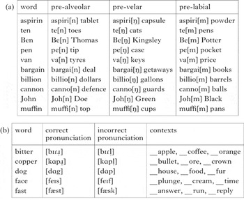
Token selection. Ten /n/-final English words were selected, and each of them was combined with a word starting with an alveolar, labial or velar plosive to form a two-word phrase. Our main interest is in the comparison of the pre-labial and pre-velar contexts, and the phrases in these contexts were therefore selected to be matched for collocational likelihood. The likelihood of the word ten given that the next word is cat (or cats or cat's) was calculated in The corpus of Contemporary American English (Davies Reference Davies2008–). The likelihood of ten given that the next word was pen (or pens or pen's) was similarly calculated. Similar values were calculated for all labial/velar pairs. A pairwise t-test was performed on these values, finding no evidence for a difference between the contexts (t(9) = 0.50, two-tailed p = 0.63). In addition to these tokens, five filler words that end with consonants other than /n/ were also selected, and used in three two-word phrases, with no specific limitation on the sound on which the second word could start. The full list of two-word phrases is given in Table I.

Table I

(a) Token stimuli and (b) filler stimuli used in Experiment 1.

Stimulus creation. Multiple repetitions of each of the token and filler phrases were recorded by a phonetically trained male native speaker of American English. Recordings were made with Praat (Boersma & Weenink Reference Boersma and Weenink2013) in a sound-attenuated room, at a sampling rate of 44.1 kHz. Phrases were produced with appropriate assimilation in the pre-velar and pre-labial contexts – i.e. pen case was produced as pe[ŋ] case. Filler tokens were recorded with the correct final consonant, and with one incorrectly produced (but acoustically related) final consonant – see Table Ib.

To identify /n/-final tokens that were produced with clear [m n ŋ], a token-selection experiment was conducted. For each /n/-final word, those three repetitions that were judged to have the most clear [m n ŋ] were identified. Each of these words were then spliced out of their two-word phrases and presented in isolation four times in random order to eight native speakers of American English. The participants’ task was to indicate whether a token ended on [m], [n] or [ŋ]. That repetition of each token that was most often identified accurately (i.e. in agreement with the actual acoustic properties of the token) was selected for use in the main experiment. The average correct identification for the selected tokens was 98%.

One repetition of each of the two pronunciations of the filler words was also selected, and spliced out of its two-word phrase. A repetition of the second word in each two-word phrase, both for the token and filler words, was selected. Each first word was then combined with its appropriate second word. In order to make the assimilated [ŋ] and [m] tokens sound natural, there was no period of silence between the first and second words when they were spliced together. Since the experimental task focuses on the initial word, the intensity of the initial word in each two-word phrase was scaled to an average of 75 dB using Praat's ‘Scale intensity’ command, while the second word was scaled to 70 dB.

Two additional copies of each recombined phrase were resynthesised using the Pitch-Synchronous Overlap and Add (PSOLA) algorithm in Praat. One copy was resynthesised to be 80% of the duration of the original phrase, and the other to be 60%. The PSOLA algorithm keeps intact the spectral properties of a token, altering only the speech rate.

Table I lists the filler and token stimuli used in the experiment. For each two-word phrase, three copies were included in the experiment (slow, faster and fastest rate) giving a total of 90 token phrases and 90 filler phrases.

Participants. Twenty-three undergraduate students from the University of Michigan were recruited as participants. All participants were native speakers of American English, and reported having no speech or hearing deficits. Participants were paid for their participation.

Procedure. Token presentation and response collection were controlled with Superlab 4 stimulus presentation software (www.superlab.com). Auditory tokens were presented over headphones at a comfortable listening level. Responses were collected through a response box connected to a MacBook laptop computer. The experiment was conducted in a sound-attenuated room. The 180 two-word phrases were each presented five times, differently randomised for each participant. Simultaneous with the auditory presentation of a phrase, participants were presented with the first word of the corresponding two-word phrase, represented in its normal spelling – i.e. even when the auditory token did not contain an accurate pronunciation of the first word, the visual stimulus was the word in its actual spelling. The task of participants was to indicate whether the phrase contained an utterance of the word presented by pushing a button on the response box. Participants were instructed to respond quickly, without sacrificing accuracy.

Hypotheses. The hypotheses were motivated in §2 above. Hypothesis 1 states that an effect of place of articulation is expected, so that more ‘yes’ responses in pre-velar than pre-labial contexts would be support for this hypothesis. Hypothesis 2 predicts that compensation should be more likely at faster speech rates. More ‘yes’ responses at the faster speech rates would provide support for this hypothesis. Hypothesis 3 claims that the effects of rate and place should be independent. The effect of speech rate should therefore be the same in pre-labial and pre-velar contexts.

3.1.2 Results

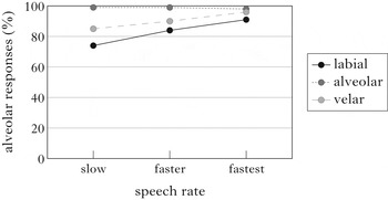
Figure 1 summarises the results of Experiment 1. Participants were very accurate at identifying the tokens that end in alveolar consonants – accuracy was 99%, 99% and 98% at the slow, faster and fastest rates. Since the main focus is on how listeners perceived place assimilated nasals, alveolar tokens were excluded from further analysis. Figure 1 also shows that participants were more likely to perceive an alveolar final token in pre-velar than pre-labial contexts (90% vs. 83%). Lastly, the figure shows a rate effect, with more alveolar percepts at faster rates (slow 80%, faster 87%, fastest 93%).

Figure 1

Response patterns in Experiment 1. The y-axis represents the percentage of ‘yes’ responses.

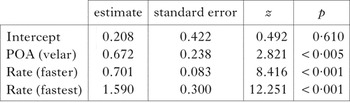
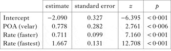
In order to assess the influence of place of articulation and speech rate on the responses a linear mixed effects model was fit to the data, using the lmer() function from the R lme4 package (Bates et al. Reference Bates, Maechler and Bolker2013). Since the response variable (yes/no) was binary, a binomial link function was used. Place of articulation (POA: velar, labial), speech rate (Rate: slow, faster, fastest) and their interaction were entered as factors, with random intercepts for participant and word, and random slopes for participants by POA and Rate. The interaction between POA and Rate was not found to be significant, and a simpler model excluding the interaction term was run. The results of this model are summarised in Table II. In this model, ‘labial’ is the reference value for POA, and ‘slow’ for Rate. The results for the intercept are hence those for the pre-labial context at the slow rate, with all of the other results expressing the relation to this category. The lmer() function does not test for the main effects of the two factors, but rather for the individual differences between the reference level and the other levels of each factor. However, since POA has only two levels, the significant difference found between the reference level ‘labial’ and ‘velar’ shows that there is a main effect for this factor.Footnote ¹ Since Rate has three levels, the results of the lmer() function cannot be used to determine whether there is a main effect of Rate. For this reason, a second model was fit to the data, excluding Rate. The results of the two models (with and without Rate) were then compared using the anova() function in R. This comparison shows that the model with Rate fits the data significantly better (χ2(9) = 656.79, p<0.001), confirming that there is also a main effect of Rate.

Table II

Results of linear mixed effects model for Experiment 1.

Experiment 1 therefore provides support for Hypothesis 1 in finding more compensation in pre-velar than pre-labial contexts, and for Hypothesis 2 in finding more compensation at faster rates. Though other research (reviewed above in §2.2) has shown that listeners can adjust their perceptual strategies to variation in speech rate, it uses longer utterances from which listeners could calculate rate. That perceptual adjustment based on rate is found in this experiment even for phrases consisting of only two words shows that listeners need very little evidence to calculate rate, and also that they can make virtually immediate perceptual adjustments to changes in speech rate. Given the lack of evidence for a significant interaction between place and rate, Hypothesis 3 is also supported.

3.2 Experiment 2

3.2.1 Methods

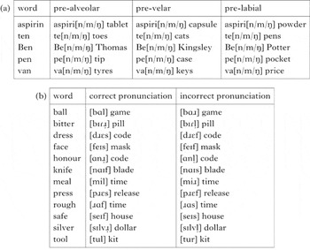
Token selection. Five /n/-final words were selected as tokens for this experiment. As in Experiment 1, each word was used in two-word phrases, with the second word starting with an alveolar, labial or velar plosive. Additionally, twelve other words were selected as filler items. Fillers all ended in a sound other than /n/, and they were also used as the first word in a two-word phrase. There was no specific limit on the sound with which the second word in the filler phrases started. The full set of tokens is given in Table III.

Table III

Stimuli used in Experiment 2: (a) /n/-final tokens; (b) other tokens.

Stimulus creation. Stimulus creation was done as in Experiment 1. Since the two-word phrases with /n/-final words used in Experiment 2 were also used in Experiment 1, the same recordings of these words were used again in Experiment 2. What was different from Experiment 1 was that the [n], [m] and [ŋ]-final pronunciations of the /n/-final words were spliced into each of the three contexts – i.e. all three pronunciations were used in a two-word phrase before a labial, alveolar or velar plosive. These phrases are listed in Table IIIa. The twelve filler phrases were recorded multiple times by the same speaker, using the same procedures. The first word in each filler phrase was produced both with the correct pronunciation and with the final consonant replaced with a different but acoustically related consonant – see Table IIIb. One example of each filler word was selected that was judged to be a clear production of the intended pronunciation. A clear production of each second word was also selected. As with the rest of the stimuli, the first words were scaled to an intensity of 75 dB and the second to 70 dB.

There was a total of 45 phrases containing /n/-final words in total: five words, each produced with a final [n], [m] or [ŋ], in pre-alveolar, pre-velar and pre-labial contexts. There were 24 additional filler phrases – two pronunciations of each of twelve words, used with the same second word. As in Experiment 1, three copies were created of each of these 69 phrases: at the original (slow) rate, at a faster rate (80% of the original) and an even faster rate (60% of the original).

Participants. Eighteen undergraduate students from the University of Michigan were recruited as participants for the experiment. All participants were native speakers of American English, who reported having no speech or hearing deficits. Participants were paid for their participation in the experiment.

Procedure. Stimulus presentation and response collection were as in Experiment 1. Tokens were presented in the same random order for all participants. Phrases with /n/-final words where the place of articulation of the /n/ agreed with the onset of the following word were presented ten times (te[n] toes, te[m] pens, te[ŋ] cats). The labial and velar tokens were the focus of the experiment, since this is where participants were expected to accommodate for place assimilation. All other tokens functioned as fillers. Phrases with a mismatch in place of articulation between the nasal and onset of the following word were each presented twice. The remaining phrases were each presented three times. The total number of tokens was therefore 756.

The task in Experiment 2 was different from that in Experiment 1. For phrases with an /n/-final word, participants were presented with three choices, indicating the three pronunciations of the /n/-final word. For example, simultaneous with the presentation of the auditory token te[m] pens, participants would see ‘ten/teng/tem’ on the monitor. Their task was to indicate which of these pronunciations was used in the auditory stimulus by pushing a button on the response box. The first visual token was always the correct pronunciation ending in [n], the second the [ŋ] pronunciation and the third the [m] pronunciation. For the other phrases, the visual presentation contained only two possible options, corresponding to the two possible pronunciations of the first word in these phrases.

Hypotheses. This section briefly explains how the hypotheses motivated in §2 are tested in this experiment, and what response patterns are expected under each of the hypotheses. Hypothesis 1 would be supported if participants selected the [n]-final answer more often in pre-velar than in pre-labial contexts. In accordance with Hypothesis 2, more [n]-final answers were expected at faster speech rates. Hypothesis 3 would receive support if the effect of speech rate was found to be the same in pre-labial and pre-velar contexts. Hypotheses 4 and 5 were tested by comparison of the results of the two experiments – see §3.3.

3.2.2 Results

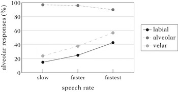
Figure 2 displays the results of Experiment 2. This figure shows the percentage of responses where listeners selected the alveolar-final option. Only phrases where the final nasal of the first word agrees in place with the onset of the second word are included – i.e. te[n] toes, te[m] pens and te[ŋ] cats. As in Experiment 1, participants were very accurate at identifying alveolar-final tokens in the pre-alveolar contexts (slow 97%, faster 96%, fastest 90%). These tokens were excluded from further analysis. The results for the pre-labial and pre-velar contexts are very similar to Experiment 1, except that overall alveolar responses were lower in Experiment 2. In agreement with Hypothesis 1, participants were more likely to perceive an alveolar final token in pre-velar than pre-labial contexts (40% vs. 28%). There was also an effect of rate, as predicted by Hypothesis 2, with more alveolar responses at faster rates (slow 20%, faster 32%, fastest 50%).

Figure 2

Response patterns in Experiment 2.

The model used in the analysis of Experiment 1 was fit to the results of Experiment 2. As before, the interaction between Rate and POA was not found to be significant, so that the final model did not include this term. The results of this model are summarised in Table IV, with ‘labial’ as the reference value for POA, and ‘slow’ for Rate. As in Experiment 1, these results show a main effect for POA. To assess the contribution of Rate, a second model was fit, excluding Rate as factor, and the results of the two models were compared using the anova() function in R. This comparison confirms that the model with Rate fits the data significantly better than the model without Rate (χ2(9) = 460.79, p<0.001).

Table IV

Results of linear mixed effects model for Experiment 2.

Like Experiment 1, Experiment 2 provides support for both Hypothesis 1, in finding more compensation in pre-velar than pre-labial contexts, and Hypothesis 2, in finding more compensation at faster speech rates. Given the lack of a significant interaction between place and rate, Hypothesis 3 is also supported. Hypotheses 4 and 5 will be evaluated in §3.3 by comparing the results between the experiments.

3.3 Comparing Experiments 1 and 2

Visual inspection of Figs 1 and 2 shows that the response patterns in the two experiments were similar – more alveolar responses in pre-velar than pre-labial contexts and at faster speech rates. There is, however, one way in which the results of the experiments diverge. Participants in Experiment 1 were much more likely to have an alveolar percept than those in Experiment 2 (87% vs. 34%), in accordance with Hypothesis 4. The figures also show that both pre-velar and pre-labial contexts were affected similarly by the inhibition of alveolar percepts in Experiment 2, suggesting that the inhibition effect is independent from the place effect, in accordance with Hypothesis 5.

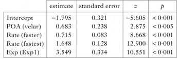
To investigate these patterns in more detail, a linear mixed effects model was fit to the data. The model contained the same factors as those used in the individual experiments, plus an additional two-level factor for Experiment (Exp: Exp1, Exp2). As before, the model contained random intercepts for word and participant, and random slopes for participants (by POA, Rate and Exp). A model with interactions between Exp, Rate and POA was initially fit to the data, but none of the interaction terms were found to contribute significantly. A simpler model without interaction terms was therefore fit. The reference level for POA was ‘labial’, for Rate it was ‘slow’, and for Exp it was ‘Exp2’. The results of this model are summarised in Table V.

Table V

Linear mixed effects model for the combined results of Experiments 1 and 2.

The significant effect of the Exp factor in the model provides confirmation for Hypothesis 4. When the /m/-final and /ŋ/-final percepts are primed, the /n/-final percept is inhibited, resulting in significantly fewer alveolar-final percepts. The lack of an interaction between the inhibition and place effects provides support for Hypothesis 5, adding additional evidence that grammatical and non-grammatical factors tend to be independent from each other. Lastly, the lack of evidence for an interaction between the rate and inhibition effects shows that these two non-grammatical factors are also independent from each other.

4.1 The data

Two possible pronunciations will be considered for each token word, the faithful pronunciation with an [n], and a pronunciation with an appropriately assimilated nasal (i.e. [m] in a pre-labial context and [ŋ] in a pre-velar context). In Experiment 1, it is not possible to know how listeners identified the word if they responded ‘no’. If a listener was presented with a token like te[m] pens, and responded ‘no’, the word could have been identified as either te[m] or te[ŋ]. It is highly unlikely, though, that a listener would have identified the word as te[ŋ]. First, such a percept would have no acoustic support from the stimulus. Secondly, te[ŋ] pens would be an ungrammatical pronunciation of ten pens. In Experiment 2, when presented with te[m] pens, participants could choose between ‘ten/teng/tem’, so that it can be determined how often listeners selected the token with an inappropriate place of articulation. When presented with a labial token, participants selected the velar response just over 1% of the time, and when presented with a velar token, they selected the labial response only 3.4% of the time. Since these responses represent less than 2% of all the data, they are not included in the model below.

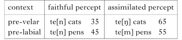
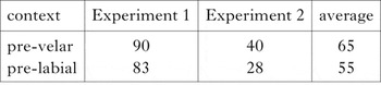
In developing the initial model, I abstract away from the influence of speech rate and lexical inhibition. This model is therefore based on the percentage of alveolar responses in pre-velar and pre-labial contexts, as averaged across the different rates and the two experiments. Table VI shows the average frequency at which listeners selected the faithful and assimilated percepts.

Table VI

Responses (%), averaged across the two experiments and three speech rates.

4.2 The basic grammar

Harmonic Grammar (Pater Reference Pater2009), like Optimality Theory, is a constraint-based model of grammar. The HG account of the experimental results relies on the constraints defined in (3). The markedness constraint Agree[place] is the driving force behind place assimilation, and Max[F]/Dep[F], rather than Ident[F], constraints will be used to regulate faithfulness. Since the assimilation rates differ in pre-labial and pre-velar contexts, the constraints must be able to differentiate between these contexts, so that Ident[place] would not be sufficient. McCarthy & Prince (Reference McCarthy and Prince1994: n. 9) already hint at this approach to featural faithfulness, while Zoll (Reference Zoll1996) represents the first formal development of this approach (albeit in a pre-Correspondence Theory Parse/Fill form).

1. (3)

   

There is a cross-linguistic implicational relationship between labial and velar triggers of nasal place assimilation: we find languages without nasal place assimilation, languages in which only velars trigger assimilation and languages in which both velars and labials trigger assimilation. However, there are no languages in which only labials trigger assimilation. A possible perceptual origin of this implication was presented in §2.1. Such universal implicational generalisations have been accounted for in two different ways in constraint-based phonology. Prince & Smolensky (Reference Prince and Smolensky1993) suggest that some constraints may be in a universally fixed ranking. To capture the implicational place assimilation, Dep[lab] could be stipulated as universally outranking Dep[vel]. However, stipulating universally fixed ranking (or weighting) relationships between constraints undermines some of the core assumptions of constraint-based phonology, where every ranking (or weighting) of constraints is usually assumed to be a possible human language. De Lacy (Reference de Lacy2004, Reference de Lacy2006) suggests an alternative approach, showing that such generalisations can be captured by defining constraints as being in a stringency relationship. This approach is adopted here. A candidate with an acquired [labial] feature therefore violates both Dep[lab] and Dep[vel]. On the other hand, a candidate with an acquired [velar] feature violates only Dep[vel].

Unlike in OT, where constraints are ranked, constraints in HG are weighted. A harmony score (H) is calculated for each candidate, based on the constraints that it violates and the weights of those constraints, according to the formula in (4). The candidate with the highest H-score is selected as the output. The formula used here is that associated with noisy HG (Jesney Reference Jesney2007, Coetzee & Pater Reference Coetzee, Pater, Goldsmith, Riggle and Yu2011) rather than classic HG (Pater Reference Pater2009). Noisy HG is to classic HG as stochastic OT (Boersma & Hayes Reference Boersma and Hayes2001) is to classic OT. The only difference between noisy HG and classic HG is that the weight of each constraint is perturbed by a small normally distributed random amount of noise every time the grammar is used. Because of these random perturbations, the H-scores for a given candidate will be slightly different every time that the grammar is used, potentially resulting in variation.

1. (4)

   

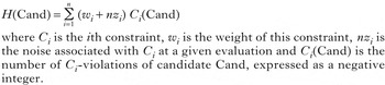
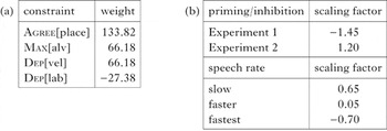
In order to determine the weights that would be needed for the constraints in (3) to produce the frequency patterns in Table VI, a learning simulation was run using a noisy HG learning algorithm implemented in Praat (for details on the learning algorithm see Coetzee & Pater Reference Coetzee and Pater2008 and Boersma & Pater Reference Boersma, Pater, McCarthy and Pater2016). The input file for the learning simulation assumed that each of the pre-labial and pre-velar contexts was encountered 100 times, with the place assimilation rates given in Table VI.Footnote ² In running the simulation, the ‘decision strategy’ was set to ‘PositiveHG’.Footnote ³ All other settings used Praat's defaults. Due to the noisiness of evaluation, slightly different weights are learned each time that the algorithm is used. The simulation was therefore run ten times; the average weights across the ten simulations are used in the rest of the paper. These weights are given in the tableau in (5), which also shows the violations incurred by each candidate.Footnote ⁴ The final column gives the H-score of each candidate, not taking into account the noisiness of the evaluation.

1. (5)

   

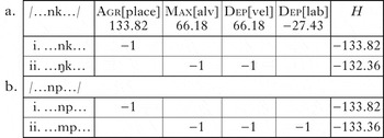
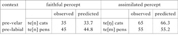
As can be seen in this tableau, the H-scores of the assimilation and faithful candidates are very close in both the pre-velar and pre-labial contexts. Consequently, once noise is factored into the evaluation, the relation between the H-scores of the two candidates may flip from one evaluation to the next, resulting in variation. Secondly, in both the pre-velar and pre-labial contexts, the H-score of the assimilation candidate is higher than that of the faithful candidate, so that assimilation should be more likely. Comparison with the frequencies in Table VI shows that this agrees with the frequency patterns in the learning data. Lastly, the H-score of the assimilation candidate in the pre-velar context is higher than that in the pre-labial context, implying that assimilation should be observed more frequently in pre-velar than pre-labial contexts – again in agreement with the patterns in Table VI. It can therefore be expected that this grammar will mimic the relative frequency patterns in Table VI. In order to verify this, Praat's ‘To output distribution’ function was used (with all settings at their default values) to determine the output patterns that this grammar would generate. Due to the noisiness of the evaluation, slightly different output patterns are predicted each time that the function is used. For this reason, the procedure was repeated ten times, and the average output patterns over the ten repetitions were calculated. The rate of assimilation predicted by this grammar is compared to the actually observed rates in Table VII, showing that the grammar accounts well for the observed frequency patterns.

Table VII

Observed and predicted rates of assimilation (%).

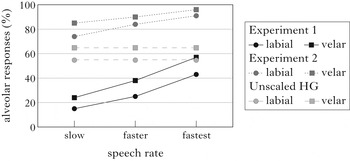
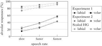
Figure 3 plots the performance of the participants in the two experiments and the predictions of the HG model. Although the HG model captures the grammatical component of the response patterns (the difference between pre-labial and pre-velar contexts), it does not capture the effect of either speech rate or lexical inhibition. The next section introduces weight scaling as a method of incorporating the contribution of these two factors into the model.

Figure 3

Comparing the performance of the unscaled HG model to the performance of the participants.

4.3 Scaling the grammar

The rate of nasal assimilation predicted by the model developed in §4.2 is higher than the actual rate in Experiment 2 and lower than the actual rate in Experiment 1. In Experiment 2, being unfaithful is less likely than predicted by the HG model, which means that the faithfulness constraints should contribute more towards determining the H-scores in modelling the results of this experiment. Following Coetzee & Kawahara (Reference Coetzee and Kawahara2013), this will be implemented by scaling the weights of faithfulness constraints up from those learned in §4.2. Conversely, the weight of faithfulness constraints will be scaled down when modelling the results of Experiment 1. The effect of rate will be accommodated in the same manner, by scaling faithfulness down for faster rates and up for slower rates.

4.3.1 Modelling inhibition

Table VIII shows the assimilation rates, averaged across different speech rates, for each of the experiments, as well as averaged between the two experiments.

Table VIII

Comparison between the assimilation rates in Experiments 1 and 2 and the overall rate (%).

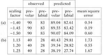
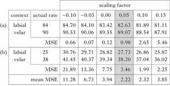
The amount by which the faithfulness constraints should be scaled up or down for the two experiments was determined by an iterative best-fit procedure. For Experiment 1, where faithfulness constraints need to be scaled down, the basic grammar weights learned above in §4.2 were scaled down in increments of 0.05. The output pattern predicted by each of these scaled versions of the grammar was then determined using Praat's ‘To output distribution’ function in the same manner as described above in §4.2. The mean square error (MSE) of these predicted assimilation rates relative to the rates actually observed in Experiment 1 was then calculated.Footnote ⁵ This procedure was repeated until the scaling factor was found that resulted in the smallest MSE. This scaling factor was found to be −1.45 for Experiment 1. A similar procedure was used for Experiment 2, except that the basic weights from §4.2 were scaled up in increments of 0.05. The scaling factor that resulted in a minimisation of the MSE for this experiment was found to be 1.20. Table IX shows the predicted assimilation rates for some different scaling factors for the two experiments, together with the MSEs associated with these scaling factors. Both (a) and (b) show the rates for the scaling factor that minimises the MSE for the particular experiment, as well as the scaling factors just below and just above this value. As the weights of the faithfulness constraints are scaled down, being unfaithful (i.e. assimilating) becomes more likely, with the opposite happening as the weights are scaled up.

Table IX

The influence of different scaling factors on the predicted assimilation rates for (a) Experiment 1 and (b) Experiment 2. The scaling factor is added to the weights of the faithfulness constraints learned in §4.2 before the output patterns of the scaled grammars are calculated.

The updated H-score formula incorporating this scaling factor is given in (6). The inhibition scaling factor, sfinhib, is −1.45 for Experiment 1 and 1.20 for Experiment 2.

1. (6)

   

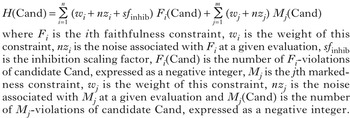
The predictions of this scaled model are much closer to the observed rates of assimilation in each of the experiments than the unscaled model from §4.2. In fact, in terms of MSE, the scaled model represents an improvement of 88% over the unscaled model (unscaled MSE = 793.42, scaled MSE = 95.37).Footnote ⁶ However, this scaled model does not take into account the effect of speech rate, and therefore predicts the same rates of assimilation for all three speech rates. In the next section, this model is augmented to incorporate the contribution of speech rate to assimilation.

4.3.2 Speech rate

The effect of speech rate is incorporated in the same way as lexical inhibition. Faithfulness constraints are scaled down for faster speech rates, resulting in higher rates of unfaithfulness (assimilation), and conversely for slower speech rates. In determining the scaling factors to be used for speech rate, the augmented model developed in §4.3.1 was used as a starting point. For Experiment 1, the starting point is therefore the weights of the faithfulness constraints, scaled down by −1.45 from the basic values learned in §4.2. Similarly, for Experiment 2, the starting values are the basic values from §4.2, scaled up by 1.20.

Different scaling factors in increments of 0.05 were tested for each of the three speech rates (slow, faster, fastest). The output patterns predicted by each of the grammars based on the 0.05 incremental scaling factors were determined by submitting each grammar ten times to Praat's ‘To output distribution’ function. The average assimilation rates for pre-velar and pre-labial contexts across these ten runs were taken to be the assimilation rates predicted by that particular scaling factor. As before, the MSE was calculated for each of the incremental 0.05 scaling factors. After this had been done separately for each of the two experimental conditions, the MSEs associated with a specific scaling factor in the two experiments were averaged. For each speech rate, the scaling factor associated with the smallest MSE averaged between the two experiments was taken to be the scaling factor associated with that particular speech rate. This procedure is illustrated in Table X, which shows the assimilation rates predicted at the ‘faster’ rate at different rate scaling factors for each of the experimental conditions. The MSE is also given for each scaling factor and each experiment separately. Finally, the last row contains the mean MSE for the two experiments at a particular scaling factor. The scaling factor that results in the lowest mean MSE for the two experiments, 0.05, is shaded. For the ‘faster’ rate, this scaling factor will be used for the ‘faster’ rate in the model developed here. The scaling factor that minimises the MSE for each of the other two speech rates was determined in the same manner. This factor was found to be −0.70 for the ‘fastest’ rate, and 0.65 for the ‘slow’ rate.

Table X

Assimilation rates predicted at different rate scaling factors for the ‘faster’ speech rate in each of the two inhibition conditions: (a) Experiment 1; (b) Experiment 2. The column corresponding to the rate scaling factor that minimises the overall MSE (0.05) is shaded. This is the scaling factor that will be used in the noisy HG model developed here.

4.3.3 Summary

The formula in (7) gives the final model, including the scaling factors for both inhibition and speech rate.

1. (7)

   

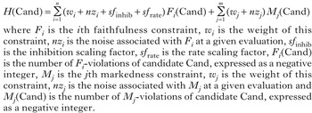
The grammar that was learned is summarised in Table XI. The constraint weights and scaling factors from this table can be substituted into the formula in (7) to find the form of the grammar to be used for any combination of speech rate and inhibition condition.

Table XI

Summary of the model: (a) constraint weights; (b) scaling factors.

Figure 4 compares the performance of this final scaled model against the response patterns of the participants in the experiment. Comparison of this figure with Fig. 3 shows that the scaled model fits the observed data much better, representing an improvement of over 99% over the unscaled model in terms of MSE.

Figure 4

Comparing the performance of the fully scaled HG model against the participant response patterns.

5.1 Grammar-dominance

As discussed in §1, in the generative tradition it has been assumed that, although both grammatical and non-grammatical factors co-determine the properties of actually produced speech, grammar takes precedence over non-grammatical factors. Grammar defines the space of possible or grammatical forms, and non-grammatical forms can only affect how frequently the forms that grammar allows are observed. Non-grammatical factors cannot override grammar or introduce new forms that are deemed ungrammatical.

Within the domain of phonological variation, there is another way in which grammar can be dominant. In addition to encoding possible grammatical forms, grammar can also impose a specific frequency relationship between two variable processes. Consider for instance variable t/d-deletion in word-final clusters in English. This process has been documented for many different varieties of English, and, as evidenced in the reviews of relevant research in Labov (Reference Labov1989) and Coetzee (Reference Coetzee2004) (see also Coetzee & Pater Reference Coetzee, Pater, Goldsmith, Riggle and Yu2011 and Coetzee & Kawahara Reference Coetzee and Kawahara2013), although dialects may differ in the absolute rate of deletion in different phonological contexts, in all dialects deletion before a consonant (e.g. west bank) is more likely than before a vowel (e.g. west end). A grammar-dominant model can do more than just specify that deletion is possible before both vowels and consonants; it can also specify that deletion before a consonant will always be more likely than before a vowel. In a constraint-based grammar (whether OT or HG) these frequency limitations follow from the specific constraints that are used to model the variable phenomenon. In modelling variable t/d-deletion, for instance, Coetzee & Kawahara (Reference Coetzee and Kawahara2013) assume a general anti-deletion constraint Max that is violated by deletion in any context, and a position-specific constraint, Max(PreV), which is violated only by deletion in prevocalic position. Since deletion in preconsonantal context violates a proper subset of the constraints violated by deletion in prevocalic position (only Max vs. Max and Max(PreV)), it follows that deletion in preconsonantal context will imply deletion in prevocalic context, but not the other way around. Anttila & Andrus (Reference Anttila and Andrus2006) show that this type of implicational generalisation (which they call a ‘T-order’) holds true of variation too, so that the possible deletion rate in preconsonantal context is guaranteed to be always at least as high as that in prevocalic context (i.e. no language with more deletion in prevocalic position is possible). Coetzee & Pater (Reference Coetzee, Pater, Goldsmith, Riggle and Yu2011: §4.4) confirm this prediction by showing that a constraint-based grammar assuming Max and Max(PreV) fails to successfully learn a grammar that can produce more deletion prevocalically that preconsonantally, even when presented with learning data that has more deletion prevocalically.

In the account of nasal place assimilation developed here, grammar similarly specifies a specific frequency relationship between assimilation in pre-labial and pre-velar contexts. The faithfulness constraints used in the account developed here were defined such that assimilation in a pre-velar context will always violate a proper subset of the constraints violated by assimilation in a pre-labial context; see (3). As shown in (8), the consequence is that the assimilation candidate in pre-velar contexts will always have a higher harmony score than the assimilation candidate in pre-labial contexts. Neither the specific weights of the constraints nor the way in which the constraint weights may be scaled by non-grammatical factors can change this relationship between the two assimilation contexts.

1. (8)

   

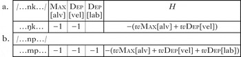
Since grammar-dominance depends on both the architecture of the grammar (how constraints interact) and the specific constraints selected, it follows that not all constraint-based grammars will have this property. For instance, if Dep[vel] were defined such that it was violated only by acquisition of a velar feature and not also by acquisition of a labial feature, a language with more assimilation in pre-labial than pre-velar contexts would be possible. Grammar-dominance therefore depends partially on the metatheory about constraints, and specifically on the strong assumption that constraints are universal and responsible for determining linguistic typology. It was the typological observation that assimilation in pre-labial position implies assimilation in pre-velar context that motivated the specific stringency formulation of the constraints Dep[lab] and Dep[vel]. The grammar-dominance illustrated here results from the way in which these constraints are defined. Grammar-dominance hence follows from assuming a strong Universal Grammar, and from a grammatical model in which UG places substantive limits on possible languages.

In another sense, grammar-dominance depends specifically on the architecture of the model. In the model assumed here, grammatical and non-grammatical factors are treated very differently. Grammatical factors are encoded in the model via specific grammatically motivated constraints, and, as shown just above, it is these constraints that are responsible for setting the limits of what a possible language is. Non-grammatical factors are implemented as merely scaling the weights associated with the grammatical constraints. Non-grammatical factors are not constraints, and cannot add or remove constraints. If non-grammatical factors were implemented as constraints on a par with grammatical constraints, or if they were allowed to remove constraints, then the strong typological limits placed on possible languages by the set of grammatical constraints would no longer hold true.

Grammar-dominance is not a property of models of phonological variation that do not assume a strong UG. As shown in §1 above, the variable rule approach, as implemented by Cedergren & Sankoff (Reference Cedergren and Sankoff1974) and widely used in variationist sociolinguistics, does not differentiate between grammatical and non-grammatical factors. The same is true of some implementations of usage-based models (Bybee Reference Bybee2001, Reference Bybee2006) and exemplar models (e.g. the papers in Gahl & Yu Reference Gahl and Yu2006, Pierrehumbert Reference Pierrehumbert, Bybee and Hopper2001). Most of these models make no formal distinction between grammatical and non-grammatical factors. In fact, in describing usage-based grammar, Bybee first defines the usage-based conceptualisation of grammar as ‘the cognitive organization of one's experience with language’ (2006: 711). Later on the same page she describes how this organisation is done as follows: ‘the general cognitive capabilities of the human brain, which allow it to categorize and sort for identity, similarity, and difference, go to work on the language events a person encounters, categorizing and entering in memory these experiences’. Grammar is the result of cognitive organisation achieved with general cognitive abilities, not with grammar- or language-specific abilities. Exactly the same cognitive abilities that organise our experience with social interactions and with our physical environment organise our experience with language. No formal distinction is made between how language and other aspects of our experience are processed or stored in the mind. If a child acquiring a language were to be exposed to a set of experiences where assimilation happens to be observed more often in pre-labial than pre-velar context, the general abilities of the mind to classify would notice this pattern, and codify this as the grammar. This view of grammar is fundamentally different from the type of approach advocated in this paper. Under the approach pursued here, there are language-specific cognitive capacities (UG represented in the constraint set, as well as in the principles for how constraints interact via their weights). Language is processed according to these principles and not with general cognitive capabilities. This places a limit on the types of grammars that can be learned.

There has been relatively little research on how grammatical and non-grammatical factors co-determine the patterns of phonological variation. The data currently available point mostly toward independence between grammatical and non-grammatical factors, and to grammar-dominance, and the model presented here has therefore been developed to have these properties. However, more research is needed to specifically probe into the relationship between grammatical and non-grammatical factors in phonological variation. If further research shows that independence or grammar-dominance does not hold true, the model presented here will have to be adapted accordingly.

5.2 More on scaling factors

In the model developed above, certain assumptions were made about how scaling factors are implemented that may be too simplistic. First, the two scaling factors (for the rate and inhibition effects) were implemented as additive. Given that no interaction was found between the rate and inhibition effects in the two experiments (see §3.3), it was warranted to implement these two effects as independent and additive. However, it is likely that various non-grammatical factors may interact with each other in complex ways. In the variationist sociolinguistic tradition, it has in fact been established that biographical characteristics of speakers can interact in such a way that age or socio-economic status may have different effects for men than women. It has also been found in this tradition that biographical characteristics of speakers may interact with things like speech style or register (see for instance the discussion on r-deletion in §1). A fully adequate model of phonological variation will therefore have to include a metatheory about how various non-grammatical factors interact with each other. One option, for instance, may be to have a separate model that combines the influence of all non-grammatical factors, and then to have only a single scaling factor in the model that reflects the combined contribution of all non-grammatical factors. More research is needed, however, about which non-grammatical factors do interact, and also about the nature of the interactions that are observed. Only once more is known about these issues will it be possible to develop a more sophisticated model of the contribution of non-grammatical factors to phonological variation.

A second assumption is that scaling factors affect faithfulness constraints only, and that they scale all faithfulness constraints alike (the weights of all faithfulness constraints are moved up or down by the same quantity) – this is in agreement with van Oostendorp's (Reference Oostendorp1997) proposal. This is most likely a too simplistic approach. It is conceivable, for instance, that the application of one variable process and the non-application of another may be associated with a specific socio-economic status. In such case, members of a speech community who belong to the specific socio-economic status group would have grammars where some faithfulness constraints are scaled down and others up. Similarly, it is not the case that all variable phenomena will be affected in the same way by things like speech rate. Though it is likely that all variable articulatory simplification phenomena (deletion, assimilation, consonantal lenition, etc.) are more likely to apply at faster than slower speech rates, the opposite pattern may well be observed in variable augmentation processes such as epenthesis (see Auger Reference Auger2001 on Vimeu Picard and Nevins Reference Nevins2007 on Brazilian Portuguese). Coetzee & Kawahara (Reference Coetzee and Kawahara2013: §5.2) make similar remarks with regard to usage frequency and variable simplification vs. augmentation processes.

The model proposed (but not developed) by Boersma & Hayes (Reference Boersma and Hayes2001: App. C) is more suited to handling a single non-grammatical factor having different impacts on different constraints. Their proposal is implemented in stochastic OT rather than noisy HG, but the basic principle is the same. They assume that non-grammatical factors (they focus on style/register, but their proposal could easily be extended to other factors as well) can move constraints up or down the hierarchy. Crucially for them, however, this is decided on a constraint-by-constraint and register-by-register basis. For each speech register, it has to be determined for each constraint whether or not it has to be moved at all, and, if it has to be moved, whether it has to be moved up or down the hierarchy and by how much. This is obviously a more powerful model of how non-grammatical factors can contribute to phonological variation than the one developed in this paper.

The correct model is most likely somewhere between that developed here and the Boersma & Hayes proposal. What is needed is a metatheory about which constraint families are affected by different non-grammatical factors, and in what way. For instance, if it is found that processes that add structure (e.g. epenthesis) are affected in one way by speech rate or usage frequency, and processes that remove structure (e.g. deletion, assimilation) are affected in a different way, then this difference has to be built into the model. More research is needed into how non-grammatical and grammatical factors co-determine patterns of phonological variation. Only once we understand these issues better will it be possible to develop a well-motivated model of how non-grammatical factors should be incorporated into a model of phonological variation. Until such time, however, the most restrictive model consistent with the data at hand is to be preferred.

5.3 Final remark

The treatment of variation in phonological theory has come a long way over the past 50 years. Where initially it was barely acknowledged, and treated as something mostly in the domain of performance and hence not part of the concern of linguistics, variation is now a central part of phonological theory. Through decades of research in variationist sociolinguistics, speech perception and production, and theoretical phonology, much is known about how phonological variation works and how it can be modelled. The time is now ripe for synthesising, and for developing a more complete model that brings together all the factors that co-determine phonological variation. This paper is one proposal for what such a comprehensive model of phonological variation could look like. It has been applied with success to the contribution of usage frequency to phonological variation by Coetzee & Kawahara (Reference Coetzee and Kawahara2013), and to the contribution of speech rate and perceptual inhibition to variation in the current paper. The model developed here is not the final word on the topic. There are many ways in which this model falls short. As more research is conducted into how grammatical and non-grammatical factors co-determine the patterns of phonological variation, the model presented here will need to be augmented, adapted or possibly even abandoned. It is my hope that this paper will be just one turn in an ongoing conversation about how to account for phonological variation in a cognitively realistic manner.