1. Introduction
In electromagnetic metallurgy, alloy particles can be separated and purified by controlling their motion under the influence of a magnetic field, which involves the transport of particles in a magnetohydrodynamic (MHD) flow (Zhang et al. Reference Zhang, Wang, Dong, Gao and Damoah2014). These particles often exhibit irregular shapes, requiring geometric approximation for theoretical analysis and numerical modelling. A common simplification is the use of spherical geometry (Shu et al. Reference Shu, Li, Sun, Zhou, Wang and Xu2000a; Kubota, Yoshikawa & Taniguchi Reference Kubota, Yoshikawa and Taniguchi2001). However, for anisotropic particles, such simplifications may lead to significant inaccuracies (Shu et al. Reference Shu, Li, Sun, Zhou, Wang and Xu2000b; Ozernykh & Kolesnichenko Reference Ozernykh and Kolesnichenko2021). In particular, elongated particles such as spheroids or cylinders are more representative of non-metallic impurities in molten metal processing, where magnetic fields are employed for impurity manipulation and removal. Several studies have reported the electromagnetic behaviour of such non-spherical particles in conductive fluids, confirming the necessity of considering their shape in MHD analyses. Ern et al. (Reference Ern, Risso, Fabre and Magnaudet2012) pointed out that particle trajectories were closely related to their wake structures. Before analysing the effects of magnetic field on particle wake structures and forces, it is essential to comprehensively understand their characteristics without a magnetic field. Unlike the sphere cases (Johnson & Patel Reference Johnson and Patel1999; Ormières & Provansal Reference Ormières and Provansal1999; Tomboulides & Orszag Reference Tomboulides and Orszag2000), the wake structure behind an inclined spheroid is more complex due to the particle’s geometric anisotropy (Fröhlich et al. Reference Fröhlich, Meinke and Schröder2020). According to Cong, Deng & Mao (Reference Cong, Deng and Mao2021), wake patterns and the forces of an inclined spheroid are governed by three dimensionless parameters, which are Reynolds number
 $\textit{Re}$
, inclination angle
 $\theta$
and aspect ratio
 $\beta$
. The characteristic length for Reynolds number is typically defined by the volume-equivalent diameter
 ${d}_e$
, which is the diameter of a sphere having the same volume as the spheroid. The inclination angle
 $\theta$
is the angle between the free-stream velocity
 $u_\infty$
and the spheroid’s long axis, as illustrated in figure 1. The aspect ratio
 $\beta$
is defined as
 $\beta = {a}/{b}$
, where
 $a$
and
 $b$
represent the semi-length of the long axis and the short axis, respectively.
Diagram of lift force in the
 $y$
-direction
 $F_{ly}$
, lift force in the
 $z$
-direction
 $F_{lz}$
, drag force
 $F_{d}$
, pitching torque in the
 $z$
-direction
 $T_{z}$
, inclination angle
 $\theta$
, the inflow
 $u_\infty$
and the magnetic field
 $B_{0}$
along the
 $x$
-direction.

Richter & Nikrityuk (Reference Richter and Nikrityuk2012) identified two critical Reynolds numbers,
 $\textit{Re}_{\textit{cr}}^{\textit{sym}}$
(approximately 200) and
 ${\textit { Re}} _{\textit{cr}}$
(200–250), for non-spherical particles in laminar flows. For an aspect ratio
 $\beta = 2$
and an inclination angle
 $\theta = 90^\circ$
, when
 $\textit{Re}$
exceeds
 $\textit{Re}_{\textit{cr}}^{\textit{sym}}$
, the wake structure transitions from a double planar symmetric state to a single planar symmetric state. As
 $\textit{Re}$
increases further beyond
 ${\mathop {\textit{Re}}\nolimits } _{\textit{cr}}$
, the previously steady wake structure becomes unsteady. Wang(Reference Wang1972, Reference Wang1974) reported that three-dimensional separation in flows past a spheroid involved a combination of a free-vortex layer and a separation bubble. These two modes were categorised as open (free-vortex layer) and closed (bubble-type) separations. Subsequent studies by Fröhlich et al. (Reference Fröhlich, Meinke and Schröder2020) observed a ‘closed–open–closed’ separation cycle at high Reynolds numbers as
 $\theta$
increases from
 $0^\circ$
to
 $90^\circ$
. Additionally, El Khoury, Andersson & Petterson (Reference El Khoury, Andersson and Petterson2012) and Wang et al. (Reference Wang, Yang, Andersson, Zhu, Liu, Wang and Lu2021) examined specific aspect ratios (
 $\beta = 6$
and
 $\beta = 2.5$
), noting that increasing
 $\textit{Re}$
resulted in a more unsteady wake structure with less symmetry and multiple frequencies, eventually leading to a chaotic state. A summary map in the
 $\{\textit{Re}, \theta \}$
plane by Wang et al. (Reference Wang, Yang, Andersson, Zhu, Liu, Wang and Lu2021) depicted this progression. Fröhlich et al. (Reference Fröhlich, Meinke and Schröder2020) noted that a smaller
 $\theta$
elongated the spheroid, preventing a closed-type recirculation bubble being induced, while larger
 $\theta$
transformed the spheroid into a blunt body, promoting the formation of a closed-type recirculation bubble. Therefore, at a smaller
 $\theta$
, such as
 $\theta = 0^\circ$
and
 $\theta = 15^\circ$
, the transition Reynolds number increased with increased
 $\beta$
, whereas at a larger
 $\theta$
, such as
 $\theta =75^\circ$
and
 $\theta = 90^\circ$
, the transition Reynolds number decreased with increased
 $\beta$
. Here, the transition Reynolds number was defined when the wake structure started to generate a closed-type recirculation bubble. Furthermore, El Khoury et al. (Reference El Khoury, Andersson and Petterson2012) identified similarities in wake structures between spheroids at
 $\theta = 90^\circ$
with a large aspect ratio (
 $\beta = 6$
) and finite-length circular cylinder flows. The influences of Reynolds number, inclination angle and aspect ratio on the wake structures of flows past a spheroid are complex and interlinked. As the Reynolds number increases, the wake structures transition through various states, becoming richer and more complex. The geometric anisotropy introduced by varying the inclination angle disrupts the separation bubble at small angles and generates a separation bubble at larger angles, leading to various wake structures in both steady and unsteady states. Additionally, the aspect ratio, coupled with the inclination angle, affects both the transition from steady to unsteady state and the symmetry of the wake structures. Increasing the aspect ratio makes the spheroid behave more like a cylinder. However, there are fewer systematic studies on the impact of aspect ratio, especially concerning its influence on the symmetry of wake structures and the transition from steady to unsteady states in the flow past an inclined spheroid.
The wake structure serves as the fundamental framework for analysing particle forces. Due to the symmetry of the wake structure, expressing the forces and torque acting on the spheroid within the investigated parameter ranges concerns three directional coefficients: drag coefficient
 $C_d$
, lift coefficient in the
 $y$
-direction
 $C_{ly}$
and in the
 $z$
-direction
 $C_{lz}$
, and torque coefficients in the
 $z$
-direction
 $C_{tz}$
, as
 \begin{equation} {C_d} = \dfrac {{{F_d}}}{{\dfrac {1}{2}\rho {u_\infty ^2 }\dfrac {{\pi {d}_e^2}}{4}}}, {C_{ly}} = \dfrac {{{F_{ly}}}}{{\dfrac {1}{2}\rho {u_\infty ^2 }\dfrac {{\pi {d}_e^2}}{4}}}, {C_{lz}} = \dfrac {{{F_{lz}}}}{{\dfrac {1}{2}\rho {u_\infty ^2 }\dfrac {{\pi {d}_e^2}}{4}}}, {C_{tz}} = \dfrac {{{T_z}}}{{\dfrac {1}{2}\rho u_\infty ^2\dfrac {{\pi {{d}_e}^3}}{8}}}. \end{equation}
Here,
 $\rho$
is the fluid density. The diagram describing lift, drag and pitching torque is presented in figure 1. The variables
 $F_{d}$
,
 $F_{ly}$
,
 $F_{lz}$
represent the forces acting in the
 $x$
,
 $y$
and
 $z$
-directions, respectively, while
 $T_{z}$
denotes the pitching torque in the
 $z$
-direction. Without a magnetic field, for the flow past an inclined spheroid under Stokes flow conditions (Happel & Brenner Reference Happel and Brenner2012), based on linearity of the Stokes equations, the influence of inclination angle
 $\theta$
to the expressions for
 $C_d$
and
 $C_{ly}$
are given as
 $${C_{d,\theta }} = {C_{d}^{0^\circ }} + \big( {{C_{d}^{90^\circ }} - {C_{d}^{0^\circ }}} \big){\sin ^2}\theta,$$
 $${C_{ly,\theta }} = \big( {{C_{d}^{90^\circ }} - {C_{d}^{0^\circ }}} \big)\sin \theta \cos \theta.$$
Here,
 $C_{d}^{0^\circ }$
and
 $C_{d}^{90^\circ }$
represent the drag coefficient at
 $\theta ={0^\circ }$
and
 $\theta ={90^\circ }$
, respectively. In incompressible planar irrotational flow, the torque coefficient
 $C_{tz}$
shows a linear dependence (Wu Reference Wu1983) as
 \begin{align} {C_{tz}} \propto \sin 2\theta. \end{align}
Sanjeevi & Padding (Reference Sanjeevi and Padding2017) demonstrated that the sine-squared drag law given in (1.2) remains valid for large Reynolds numbers (up to 2000). However, due to the nonlinear effects brought by high Reynolds numbers, significant changes in maximum values and phase shifts exist in the correlation between
 $C_{ly}$
,
 $C_{tz}$
and the inclination angle
 $\theta$
(Zastawny et al. Reference Zastawny, Mallouppas, Zhao and Van Wachem2012; Sanjeevi & Padding Reference Sanjeevi and Padding2017; Fröhlich et al. Reference Fröhlich, Meinke and Schröder2020). These deviations create large errors when using (1.3)–(1.4) to predict
 $C_{ly}$
and
 $C_{tz}$
. Consequently, (1.3)–(1.4) are corrected as
 $${C_{ly}} = ( {C_{d}^{90^ \circ} - {C_{d}^{0^ \circ}}}){f_l}( {{\mathop {\textit{Re}}\nolimits},\beta})\sin({2{f_{l,\theta }}({\theta ,{\mathop {\textit{Re}}\nolimits } ,\beta })}),$$
 $${C_{tz}} = {C_{tz,\textit{max}}}\left ( {\textit{Re},\beta } \right )\sin ( {2{f_{t,\theta }}( {\theta ,\textit{Re},\beta } )} ).$$
Here,
 $f_{l}$
and
 $f_{l,\theta}$
, denote the correction funcutions related to shape and Reynolds number, corresponding respectively to the variation in the maximum value and the phase shift of
 $C_{ly}$
.
 $C_{tz,max}$
and
 $f_{t,\theta}$
represent the maximum value and the correction functions for shape and Reynolds number affecting the phase shift of
 $C_{tz}$
. In addition, compared with Stokes flow, the nonlinear effects introduced by high Reynolds numbers and the complex interactions between Reynolds number and aspect ratio require corrections for
 $C_{d}^{0^\circ }$
and
 $C_{d}^{90^\circ }$
(Zastawny et al. Reference Zastawny, Mallouppas, Zhao and Van Wachem2012; Ouchene et al. Reference Ouchene, Khalij, Arcen and Tanière2016; Sanjeevi & Padding Reference Sanjeevi and Padding2017; Fröhlich et al. Reference Fröhlich, Meinke and Schröder2020; Chen et al. Reference Chen, Jiang, Xiong, Wei, Fang and Wang2021; Wang et al. Reference Wang, Yang, Andersson, Zhu, Liu, Wang and Lu2021). These corrections are summarised in the form of:
 \begin{align} {C_{d}^{\theta _i}} = {C_{d,\textit{Stokes}}^{\theta _i}}{f_d}\left ( {{\mathop {\textit{Re}}\nolimits } ,\beta } \right )\!, {\theta _i} = {0^ \circ },{90^ \circ }. \end{align}
Here,
 ${f_d} ({\mathop {\textit{Re}}\nolimits , \beta })$
represents the shape and Reynolds number correction functions. Jeffery (Reference Jeffery1922) derived and defined
 $C_{d}^{0^\circ }$
and
 $C_{d}^{90^\circ }$
in Stokes flow as
 $C_{d, {\textit{Stokes}}}^{0^\circ }$
and
 $C_{d, {\textit{Stokes}}}^{90^\circ }$
in (C1)–(C2). Since the analytical expressions for the force or torque coefficients under multi-parameter control cannot be directly derived, table 1 lists some force expressions which typically contain a large number of fitting parameters, such as those with approximately 6–12 parameters. However, even with a significant number of fitting factors, the deviation of
 $C_d$
was up to 20 %, while the deviation of
 $C_{ly}$
and
 $C_{tz}$
were up to 25 % for the correlation function provided by Ouchene et al. (Reference Ouchene, Khalij, Arcen and Tanière2016). Furthermore,
 $C_{tz}$
tends to be less accurate than
 $C_d$
and
 $C_{ly}$
due to its higher sensitivity to surface stress distribution in Cui et al. (Reference Cui, Wang, Jiang and Zhao2022):
Some of orientation-dependent expressions for drag coefficients
 $C_d$
, lift coefficients
 $C_l$
and torque coefficients
 $C_{t}$
in previous researches with application scope and parameter number without the magnetic field in different Reynolds numbers, aspect ratios and inclination angles.

With a magnetic field, an additional dimensionless parameter, the interaction parameter
 $N$
, is introduced to quantify the ratio between electromagnetic and inertial forces. The motion of a conducting fluid, when not aligned with the magnetic field, induces electrical currents. These currents interact with the magnetic field to produce MHD forces known as the Lorentz force, significantly impacting wake structures and forces, as presented by Davidson (Reference Davidson2017). Experiments (Lahjomri, Capéran & Alemany Reference Lahjomri, Capéran and Alemany1993) and numerical simulations (Mutschke et al. Reference Mutschke, Gerbeth, Shatrov and Tomboulides2001) have examined flows past a cylinder under the influence of a streamwise magnetic field. They found that the vortex narrowed and vortex shedding was suppressed, eventually leading to a transition to a two-dimensional flow as the interaction parameter
 $N$
increased. Additionally, magnetic fields applied in different directions, such as the transverse (Frank, Barleon & Müller Reference Frank, Barleon and Müller2001; Kanaris et al. Reference Kanaris, Albets, Grigoriadis and Kassinos2013) and along the cylinder axis (Kolesnikov & Tsinober Reference Kolesnikov and Tsinober1974), had a stronger influence on the wake structures compared with the streamwise magnetic field. Similar suppressing phenomena were observed in the case of flow past a sphere in a magnetic field. However, the wake structure evolution differs from that of a cylinder. Experiments by Yonas (Reference Yonas1967) showed that flows past a sphere in a relatively weak magnetic field could completely suppress the dominant frequency. Similar results were reported by Maxworthy (Reference Maxworthy1962), indicating that applying a magnetic field transformed wake structure behind the sphere from an oscillatory to a non-oscillatory wake. Pan et al. (Reference Pan, Zhang and Ni2018, Reference Pan, Zhang and Ni2019) classified five wake patterns in a streamwise magnetic field and three wake patterns in a transverse magnetic field based on their state and symmetry, investigating the mechanism of the transformation between these wake patterns within the laminar regime (
 $Re\leqslant 300$
). They revealed and summarised a ‘reversion phenomenon’, which described the wake structure of the sphere at a higher
 $\textit{Re}$
and a certain
 $N$
corresponding to a lower
 $\textit{Re}$
with a lower
 $N$
. These studies demonstrate that the magnetic field significantly influences the wake structure of both cylinder and sphere. Due to the geometric similarities of a spheroid to a cylinder and a sphere, the magnetic field is expected to have a significant effect on the wake structure of the spheroid. This effect is one of the primary focuses of the present paper.
Regarding the effect of magnetic fields on the forces acting on a particle, Yonas (Reference Yonas1967) measured the drag on a sphere in conductive sodium under a directed magnetic field. They observed a linear relationship between the drag and the square root of the interaction parameter under strong streamwise magnetic fields as
 \begin{equation} {{C_d} \sim \sqrt N }. \end{equation}
Similarly, Sekhar, Sivakumar & Ravi Kumar (Reference Sekhar, Sivakumar and Ravi Kumar2005) found the same law. They explained this behaviour by noting a general increase in upstream base pressure and a decrease in downstream base pressure affected by the magnetic field. Here, the base pressure refers to the pressure measured at specific locations on the particle surface, particularly at the upstream and downstream stagnation points with respect to the flow direction. Pan et al.(Reference Pan, Zhang and Ni2018, Reference Pan, Zhang and Ni2019) derived (1.8) from an energy perspective under the influence of strong magnetic fields (
 $N \geqslant 1$
) in both streamwise and transverse directions, explaining that the linear relationship
 ${C_d} \sim \sqrt N$
is available for particles of arbitrary shapes and for different orientations of the magnetic field. However, under a weak transverse magnetic field (
 $N \lt 1$
), Delacroix & Davoust (Reference Delacroix and Davoust2018) and Pan, Zhang & Ni (Reference Pan, Zhang and Ni2019) found that the drag coefficient is proportional to
 $N^{0.65}$
. In summary, the magnetic field significantly affects the force and torque on the particle. Therefore, exploring the expressions of the force and torque coefficients is another primary focus of this paper.
Previous studies on flows past a particle have highlighted substantial disparities in wake structures and forces among various particle geometries. However, the influence of magnetic fields on different particle shapes remains relatively unexplored, particularly regarding insulated spheroids in MHD flows. This study employs three-dimensional simulations to analyse wake structures and derive expressions for force and torque coefficients for flows past an inclined insulated spheroid with a streamwise magnetic field. Based on this, the paper is organised as follows. Section 2 describes the mathematical model and numerical methods. Section 3 presents numerical results for the wake structure and expressions for lift, drag and torque coefficients of the flows past an inclined spheroid influenced by a streamwise magnetic field. Finally, a summary is provided in § 4.
2. Mathematical model and numerical method
The computational approach for simulating flows past an inclined insulated spheroid in a streamwise magnetic field is similar to the numerical technique for a sphere case proposed by Pan et al. (Reference Pan, Zhang and Ni2019), which will be adopted in this study. For most cases of solid particle two-phase liquid metal flow in industrial applications, the length scale of these particles is typically very small, approximately
 $10^{ - 6}$
–
 $10^{ - 3}$
(Ku et al. Reference Ku, Wang, Wang and Lei2024). The magnetic Reynolds number
 $Rm = {\mu }\sigma {{d}_e}{u_\infty } \sim O({{{10}^{ - 3}}})$
. This parameter estimates the relative effects of advection or induction of a magnetic field by the motion of a conducting medium to the magnetic diffusion to be very small; the induced magnetic field is negligible compared with the external field. Here,
 $\mu$
and
 $\sigma$
are the magnetic permeability and electrical conductivity of the fluid, respectively. Hence, the flow can be simulated by using a quasistatic approximation in Moreau (Reference Moreau1990) and Davidson (Reference Davidson2017). Under this approximation, the dimensionless flow equations can be written as
 $$\frac {{\partial {\boldsymbol{u}}}}{{\partial t}} + \left ( {{\boldsymbol{u}} \boldsymbol{\cdot }\boldsymbol{\nabla }} \right ){\boldsymbol{u}} = - \boldsymbol{\nabla }p + \frac {1}{{{\mathop {\textit{Re}}\nolimits } }}{\boldsymbol{\nabla} ^2}{\boldsymbol{u}} + N\left ( {{\boldsymbol{J}} \times {\boldsymbol{B}}} \right )\!,$$
 $${\boldsymbol{\nabla }\boldsymbol{\cdot }{\boldsymbol{u}} = 0},$$
 $$\boldsymbol{\nabla }\boldsymbol{\cdot }{\boldsymbol{J}} = 0.$$
Associating the solenoidal current field in (2.3) and Ohm’s law in
 ${\boldsymbol{J}} = - \boldsymbol{\nabla }\phi + {\boldsymbol{u}} \times {\boldsymbol{B}}$
, a Poisson equation for the electric potential can be derived as
 \begin{equation} \boldsymbol{\nabla }\boldsymbol{\cdot }\boldsymbol{\nabla }\phi = \boldsymbol{\nabla }\boldsymbol{\cdot }\left ( {{\boldsymbol{u}} \times {\boldsymbol{B}}} \right )\!. \end{equation}
The dimensionless variables, time
 $t$
, velocity
 $\boldsymbol{u}$
, pressure
 $p$
, current density
 $\boldsymbol{J}$
, imposed magnetic field
 $\boldsymbol{B}$
, and electric potential
 $\phi$
, are scaled by
 ${{d}_e}/{u_\infty }$
,
 $u_\infty$
,
 $\rho u_\infty ^2$
,
 $\sigma {u_\infty }{B_0}$
,
 $B_0$
and
 ${{d}_e}{u_\infty }{B_0}$
, respectively. Here,
 $B_0$
is the intensity of magnetic field. Two dimensionless parameters introduced in the momentum (2.1) are the Reynolds number
 $ Re= {{{u_\infty }{{d}_e}} \mathord {\left / {\vphantom {{{u_\infty }{{d}_e}} \nu }} \right . }\! \nu }$
to measure the ratio of inertial to viscous forces and the interaction parameter
 $N = {{\sigma {{d}_e}B_0^2} \mathord {\left / {\vphantom {{\sigma {{d}_e}B_0^2} {\rho {u_\infty }}}} \right . }\! {\rho {u_\infty }}}$
to measure the ratio of electromagnetic to inertial forces. Here,
 $\nu$
is the kinematic viscosity.
Schematic for the flow configuration. (a) Computational domain. (b) Grid expanded view in the vicinity of the spheroid in
 $xoy$
plane.

Figure 2(a) shows the flow configuration. An inclined spheroid is placed along the axis of a rectangular duct which has size
 ${28}{{d}_e} \times {20}{{d}_e} \times {20}{{d}_e}$
, with a uniform free stream and a streamwise magnetic field both along the
 $x$
-axis. The inlet is located
 ${8}{{d}_e}$
upstream of the spheroid and the outlet is located
 ${20}{{d}_e}$
behind the spheroid. This domain size is chosen to ensure a reasonable computational cost while minimising the distortion of the flow structure by the external boundary conditions. A uniform velocity is given at the inlet, a convective boundary condition is applied at the outlet, free-slip conditions are imposed on the sidewalls, and a no-slip and insulated boundary condition is enforced on the surface of the spheroid. For the MHD flow, the electric potential boundaries should be specified for the electric potential governing equation. All electric potential boundary conditions proposed by Mück et al. (Reference Mück, Günther, Müller and Bühler2000) can be set as
 \begin{equation} \frac {{\partial \phi }}{{\partial {\boldsymbol{n}}}} = \left ( {{\boldsymbol{u}} \times {\boldsymbol{B}}} \right ) \boldsymbol{\cdot }{\boldsymbol{n}}. \end{equation}
Here,
 $\boldsymbol{n}$
is the normal vector of the spheroid surface. The boundary condition of (2.5) is derived by projecting Ohm’s law onto the fluid–wall interface, under the assumption of electrically insulating boundaries.
Establishing appropriate mesh settings is essential for simulating flows past a spheroid in a streamwise magnetic field. This study focuses primarily on resolving the boundary layer and wake region near the spheroid, which requires higher grid resolution in these critical zones. In the context of MHD channel flow (Molokov, Moreau & Moffatt (Reference Molokov, Moreau and Moffatt2007)), the thicknesses of the Hartmann layers perpendicular to the magnetic field and the Shercliff layers parallel to the magnetic field on a flat wall are scaled as
 ${\delta _ \bot } \sim O({H{a^{ - 1}}} )$
and
 ${\delta _\parallel }\sim O({H{a^{ - {1}/{2}}}} )$
, respectively. With a maximum Hartmann number
 $ Ha \approx 50$
, the Shercliff boundary layer is significantly thicker than the Hartmann boundary layer. However, these scaling relationships are based on flat wall situations and may not directly apply to spheroidal geometries. Previous research has not specifically addressed flow simulations around a spheroid in a streamwise magnetic field, except for the approach by Pan, Zhang & Ni (Reference Pan, Zhang and Ni2018), who determined a grid spacing
 ${\delta _{\textit{min} }} = {0.01{d}_e}$
based on the nearest grid point to the spheroid’s surface, confirming its accuracy. Figure 2(b) gives a detailed grid resolution near the spheroid. To ensure adequate resolution within the boundary layer, a minimum spacing of
 $0.01{d}_e$
and
 $0.005{d}_e$
are adopted, described in table 2. The cases with
 $\beta =6$
,
 $Re=250$
,
 ${\theta } = {45^ \circ }$
and
 $\theta = {90^ \circ }$
at
 $N=0$
and
 $N=10$
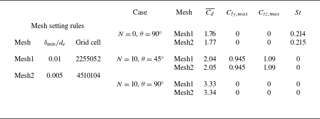
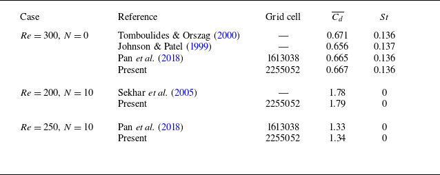
are tested first. Based on these results, demonstrated in table 2, Mesh1 is chosen and it is sufficient to resolve wake flow behind the inclined spheroid. Subsequently, flows past a sphere with and without a magnetic field for steady and unsteady cases are tested. The results, demonstrated in table 3, confirm the accuracy of the numerical method and boundary conditions in resolving cases of flows past a particle in a magnetic field. Later, the cases with
 $\beta =6$
,
 $Re=272$
,
 $\theta = {90^ \circ }$
and
 $\beta =2.5$
,
 $Re=100$
,
 ${\theta } = {45^ \circ }$
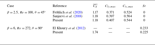
without a magnetic field are selected for comparison with previous studies. The results, presented in table 4, prove the accuracy of the numerical method and confirm the sufficiency of Mesh1 for resolving the present simulations.
Grid independence test for flows past an inclined spheroid at
 $\beta = 6$
,
 $Re=250$
. Here,
 $\delta _{\textit{min}}$
is the first layer thickness of the spheroid surface grid. The Strouhal number
 $St$
is defined as
 $St = {{f{{d}_e}} /{{u_\infty }}}$
, where
 $f$
is the vortex shedding frequency.
 $\overline {{C_d}}$
is the average value of
 $C_d$
.
 $C_{ly,max}$
is the maximum value of
 $C_{ly}$
.

Numerical method and boundary conditions test for flows past a sphere with a magnetic field.

Numerical method and boundary conditions test for flows past an inclined spheroid without a magnetic field.

3. Results
This section aims to investigate the effects of the streamwise magnetic field on wake patterns and forces in flows past an insulated spheroid. A total of 1150 data points are computed for all combinations within parameter range:
 $50 \leqslant \textit{Re} \leqslant 250$
,
 $1.5 \leqslant \beta \leqslant 6$
,
 ${0^ \circ } \leqslant \theta \leqslant {90^ \circ }$
and
 $0 \leqslant N \leqslant 10$
. The streamwise magnetic field is applied from the beginning of the simulation. The flow is simulated for long enough time until it reaches statistical stability.
3.1. The wake structures affected by a streamwise magnetic field
With the influence of
 $\textit{Re}$
,
 $\beta$
,
 $\theta$
,
 $N$
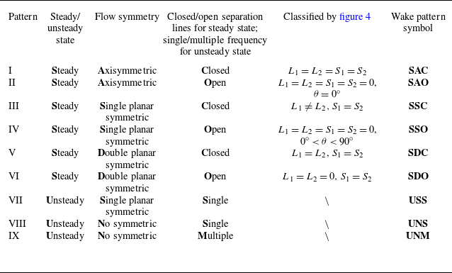
, the wake structures behind the spheroid have a rich evolution. In order to briefly describe the characteristic of these wake structures, a total of nine wake patterns are summarised. These wake patterns are classified by three aspects: steady/unsteady state, flow symmetry, and closed/open separation lines for steady states and single/multiple frequency for unsteady states. Lighthill (Reference Lighthill and Rosenhead1963) proposed the convergence of the skin-friction lines to be the criterion of three-dimensional flow separation. The skin-friction lines are employed to analyse flow traces in the rear of the spheroid for six steady state patterns while the characteristics of the three unsteady patterns are revealed by plotting isosurfaces of the Q-function (Jeong & Hussain Reference Jeong and Hussain1995), as shown in figure 3. To intuitively distinguish the characteristics of these wake patterns, they are summarised into a schematic diagram of the projection streamline on the plane with the relative sizes of
 $L_1$
,
 $L_2$
,
 $S_1$
and
 $S_2$
in figure 4. Here,
 $L_1$
and
 $L_2$
represent a pair of counter-rotating spirals projected on the
 $xoy$
plane, while
 $S_1$
and
 $S_2$
denote a pair of counter-rotating spirals projected on the
 $xoz$
plane. A detailed description of the characteristics of nine different wake structures is given in table 5. Under the effects of
 $\textit{Re}$
,
 $\beta$
,
 $\theta$
,
 $N$
, considering the geometric symmetry of particles with different spheroid placement in the flow, such as axisymmetric at
 $\theta = {0^ \circ }$
, single planar symmetric at
 ${0^\circ } \lt \theta \lt {90^\circ }$
and double planar symmetric at
 $\theta = {90^ \circ }$
, three typical placements with special angles,
 $\theta = {0^ \circ , 60^ \circ , 90^ \circ }$
, are chosen to study the effect of the streamwise magnetic field on wake structures.
Nine different wake patterns classified by table 5: (a) SAC, (b) SAO, (c) SSC, (d) SSO, (e) SDC, ( f) SDO, (g) USS, (h) UNS, (i) UNM.

A detailed description of the characteristics of nine different wake patterns. Here,
 $L_1$
and
 $L_2$
are a pair of counter-rotating vortices in the
 $xoy$
plane, and
 $S_1$
and
 $S_2$
are a pair of counter-rotating vortices in the
 $xoz$
plane in figure 4.

A feeding spiral model with competing upstream meridional and latitudinal flows around the spheroid, abstracted from three-dimensional flow simulations. (a) The actual three-dimensional streamlines of
 $\beta = 2$
, Re = 250,
 $N = 0$
,
 $\theta = {90^\circ }$
. (b) The schematic feeding spiral model.
 $L_1$
and
 $L_2$
are a pair of counter-rotating spirals projected in the
 $xoy$
plane.
 $S_1$
and
 $S_2$
are a pair of counter-rotating spirals projected in the
 $xoz$
plane.

3.1.1. Impact of the aspect ratio for unsteady patterns without a magnetic field
Previous research has established an interlinking relationship between
 $\beta$
and the inclination angle
 $\theta$
. In this study, we explore a more extensive range of aspect ratio to discover the evolution and mechanism of wake structures. To demonstrate the effect of the aspect ratio
 $\beta$
on the evolution of the wake structure, figure 5 demonstrates the relative stagnation point positions and the shedding frequency, while figure 6 shows the streamline projections in the
 $xoy$
and
 $xoz$
planes, as well as the lift force coefficients over time. These streamline projections are summarised in figure 4 to explain the influence of
 $\beta$
. Extensive analyses (Johnson & Patel Reference Johnson and Patel1999; Ghidersa & Dušek Reference Ghidersa and Dušek2000; Tomboulides & Orszag Reference Tomboulides and Orszag2000) of flows past a sphere (
 $\beta = 1$
) at
 $Re=250$
revealed a Steady, Single planar symmetric and Closed separation lines (SSC) pattern, as shown in figure 6(a). Since the Reynolds number exceeds the first critical number, the original axisymmetric wake structure is disrupted into a planar symmetric one. Based on the numerical simulation results shown in figure 4(a), three typical upstream flow types, denoted as FM, SM and SL, are abstracted from the three-dimensional streamlines associated with the spiral pairs
 $L_1$
,
 $L_2$
,
 $S_1$
and
 $S_2$
. These flow types can be categorised as follows:
-
(i) FM: the upstream flows from the meridian of the spheroid, flowing around the
 $L_2$
spiral, and feeding the
$L_1$
spiral.
-
(ii) SM: the upstream flows consist of meridional components from the side of the spheroid, also flowing around the
$L_2$
spiral and feeding the
$L_1$
spiral. -
(iii) SL: the upstream flows consist of latitudinal components from the side of the spheroid, feeding the spiral pair of
$S_1$
and
$S_2$
.


These three upstream flow types form the basis of the feeding spiral model, as illustrated in figure 4(b), which explains the evolution of the wake structure with increasing aspect ratio
 $\beta$
. Notably, the upper flows exert a shear effect on
 $L_1$
rather than directly feeding it. For instance, in flow past a sphere (
 $\beta = 1$
), the wake structure remains axisymmetric at low Reynolds numbers (
 $\textit{Re} \lt 210$
), and the FM flow does not flow around
 $L_2$
to feed
 $L_1$
. When
 $\textit{Re}$
increases to 250, exceeding the first critical Reynolds number (
 $\textit{Re}_{{\textit{cr}}} \approx 210$
), the wake transitions to a Steady, Single planar symmetric and Closed separation lines (SSC) pattern (Johnson & Patel Reference Johnson and Patel1999; Ghidersa & Dušek Reference Ghidersa and Dušek2000; Tomboulides & Orszag Reference Tomboulides and Orszag2000). At this point, the FM flow begins to flow around the
 $L_2$
spiral and feed the
 $L_1$
spiral, as shown in figure 6(a).
It is noted that, to ensure that
 ${d}_e$
in the definition of
 $\textit{Re}$
remains the same, increasing
 $\beta$
elongates the spheroid’s long axis and shortens its short axis. As
 $\beta$
increases to 1.5, the spheroid takes on a spherical-like shape. The increased centre distance between the
 $L_1$
and
 $L_2$
spirals requires more upstream inertia of the flow around the spheroid’s meridian to feed the
 $L_1$
spiral, but the FM flow feeding the
 $L_1$
spiral will decrease. However, the changed curved surface of the body enhances SM flow to gain more upstream inertia of the flow to feed the
 $L_1$
spiral along the meridians of the spheroid, ultimately leading to the shedding of the
 $L_1$
spiral, as shown in figure 6(b). At this stage, the shorten distance between the spiral pair of
 $S_1$
and
 $S_2$
increases the flushed flow on the short-axis side. That makes them suffer a bigger pushing effect, though it remains insufficient to cause alternate shedding of
 $S_1$
and
 $S_2$
spirals. Instead,
 $S_1$
and
 $S_2$
spirals shift toward the
 $z$
-axis, leading to a small asymmetry. Since only the
 $L_1$
spiral sheds behind the spheroid, the relative stagnation point position oscillates along the
 $y$
-axis with a slight shift in the
 $z$
-direction, as illustrated in figure 5(b). The wake is asymmetric and displays a single shedding frequency. This indicates that the aspect ratio has exceeded a critical value, transforming the wake structure into the Unsteady, No symmetric and Single shedding frequency (UNS) pattern.
Influence of aspect ratio
 $\beta$
on wake patterns without a magnetic field at
 $Re=250$
,
 $\theta ={90^ \circ }$
. (a) Definition of the location position coordinates of the stagnation point. (b) Relative location coordinates of the stagnation point in one period of time to show the symmetry and the vortex shedding plane of the wake structure in the unsteady state. The connecting lines reflect the general trend of motion but do not represent continuous trajectories. (c) Vortex shedding Strouhal number
 $St$
.

Influence of aspect ratio
 $\beta$
on wake patterns without a magnetic field at
 $Re=250$
,
 $\theta ={90^ \circ }$
, described by normalised pressure contours and streamlines projected onto the
 $xoy$
and
 $xoz$
planes, as well as the time evolution of lift force coefficients. The normalised pressure P is scaled with
 $({1}/{2}){\rho}{u_\infty^2}$
. Red arrows denote vortex shedding.

As
 $\beta$
increases to 2, the spheroid is more slim and cylindrical in shape, causing partial SM flow to transfer to the SL flow. Moreover, the increasing centre distance between
 $L_1$
and
 $L_2$
spirals reduces the FM flow feeding the
 $L_1$
spiral. These two effects cause less upstream flow to feed
 $L_1$
spiral shedding, as indicated by the smaller oscillation amplitude of
 $C_{ly}$
compared with the case of
 $\beta = 1.5$
in figure 6(b). Meanwhile, the further reduced centre distance between
 $S_1$
and
 $S_2$
spirals increases the flushed flow on the short-axis side. That enhances the pushing effect, making the SL flow sufficiently strong to initiate alternate shedding of the
 $S_1$
and
 $S_2$
spirals behind the spheroid, as shown in figure 6(c). This alternate shedding leads to interactions between the
 $L_1$
spiral and the spiral pair of
 $S_1$
and
 $S_2$
, transforming the wake structure from a single frequency to multiple frequency. Consequently, the relative stagnation point position begins to oscillate along the
 $z$
-axis while continuing its oscillation along the
 $y$
-axis in figure 5(b). Now, the wake is the Unsteady, No symmetric and Multiple shedding frequency (UNM) pattern. The interaction between the
 $L_1$
spiral and the spiral pair of
 $S_1$
and
 $S_2$
causes the
 $L_1$
spiral to take less upstream flow, reducing its oscillation amplitude and frequency of the
 $L_1$
spiral shedding compared with the case with
 $\beta = 1.5$
, where only the
 $L_1$
spiral sheds. As a result, the Strouhal number
 $St$
of the
 $L_1$
spiral decreases as
 $\beta$
increases from 1.5 to 2, as shown by the circle symbol in figure 5(c).
As
 $\beta$
increases to 3, the spheroid gradually transitions from spheroidal to cylindrical. The reduced FM and SM flows cannot keep the
 $L_1$
spiral shedding. Instead, they make
 $L_1$
and
 $L_2$
spirals shift from the origin to the y-axis, as shown in figure 6(d). Meanwhile, the continued increase of the flushed flow on the short-axis side increases the alternate shedding of the spiral pair of
 $S_1$
and
 $S_2$
. Since only the spiral pair of
 $S_1$
and
 $S_2$
sheds behind the spheroid, the relative stagnation point position oscillates along the
 $z$
-axis with a shift in the
 $y$
-direction, as shown in figure 5(b). The wake is asymmetric and displays a single shedding frequency, indicating that the wake structure has reverted to the UNS pattern. Note that compared with
 $\beta = 1.5$
, the shedding spiral shifts from the
 $L_1$
spiral to the spiral pair of
 $S_1$
and
 $S_2$
. Since the
 $L_1$
spiral shedding length on the long-axis side is longer than the spiral pair of
 $S_1$
and
 $S_2$
on the short-axis side, the
 $St$
of
 $\beta = 3$
is larger than that of
 $\beta = 1.5$
. Furthermore, since the flushed flow on the short-axis side of
 $\beta = 3$
is stronger than that of
 $\beta = 2$
, the
 $St$
of the spiral pair
 $S_1$
and
 $S_2$
for
 $\beta = 3$
is larger, as shown by the square symbol in figure 5(c).
As
 $\beta$
increases to 6, the spheroid begins to resemble a finite cylinder, causing SM flow to converge to zero and the FM flow to continue to decline, making it insufficient to send upstream flow around the
 $L_2$
spiral to feed the
 $L_1$
spiral. This results in the
 $L_2$
spiral shifting downward, causing the
 $L_1$
spiral to enlarge and the
 $L_2$
spiral to reduce until
 ${L_1} = {L_2}$
, which indicate that the wake structure regains the symmetry in the
 $xoz$
plane. This can be demonstrated in figure 6(e). Since only the spiral pair of
 $S_1$
and
 $S_2$
sheds behind the spheroid, the relative stagnation point position oscillates along the
 $z$
-axis, as illustrated in figure 5(b). The wake is single planner symmetric and displays a single shedding frequency, indicating that the wake structure has reverted to the USS pattern. Meanwhile, the continued increase of the flushed flow on the short-axis side intensifies the alternate shedding of the spiral pair
 $S_1$
and
 $S_2$
further, making
 $St$
of
 $\beta = 6$
larger than that of
 $\beta = 3$
, as shown in figure 5(c).
Enhancing
 $\beta$
increases the distance between the
 $L_1$
and
 $L_2$
spirals, while reducing the distance between the
 $S_1$
and
 $S_2$
spirals. That redistributes the upstream flows, including FM, SM and SL flows, resulting in a transformation in wake pattern topology: from Steady state, Single planar symmetric and Closed separation lines (SSC) to Unsteady state, No symmetric and Single frequency (UNS), followed by Unsteady state, No symmetric and Multiple frequency (UNM), then back to Unsteady state, No symmetric and Single frequency (UNS), and to Unsteady state, Single planar symmetric and Single frequency (USS) as
 $\beta$
increases from 1 to 6 (illustrated in figures 5b and 6). Generally, increasing
 $\beta$
increases
 $St$
(except for
 $\beta = 2$
), as demonstrated in figure 5(c). As
 $\beta$
continues to rise, the spheroid progressively approaches the geometry of a two-dimensional cylinder. Keeping the inflow velocity constant, increasing
 $\beta$
decreases the short-axis of the spheroid. When using the radius of the short-axis to calculate the short-axis Reynolds number
 ${Re}_{s} = u_{\infty}2b/\nu$
, this Reynolds number will approach to 47, which is consistent with the critical Reynolds number of a cylinder (Williamson Reference Williamson1996). Notably, as
 $\beta$
increases, the spheroid represents a transitional state from a sphere (
 $\beta = 1$
) to a cylinder (
 $\beta \to \infty$
), highlighting its unique role in bridging these two geometric extremes. Therefore, it can be postulated that the spheroid will eventually revert to a steady state pattern as
 $\beta$
continues to increase until reaching a critical value of approximately
 $\beta = 160$
, which corresponds to
 $Re_s = 47$
. An extended case of
 $\beta = 15$
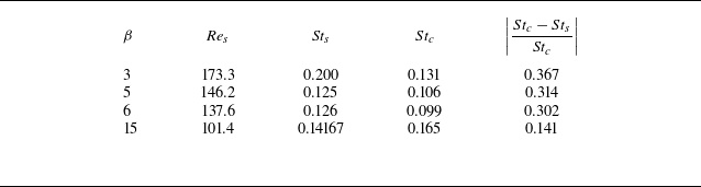
further supports this hypothesis with detailed discussion and quantitative comparison provided in Appendix A.
3.1.2. Impact of the streamwise magnetic field on a spheroid inclined by
$\theta = {0^ \circ }$

The transformation from SAO to SAC patterns can be observed in Fröhlich et al. (Reference Fröhlich, Meinke and Schröder2020) at
 $\beta = 2$
,
 $\theta = {0^ \circ }$
when
 $\textit{Re}$
increases from 50 to 100 without a magnetic field. In this section, to investigate the mechanism of variation of these two wake patterns under the influence of a streamwise magnetic field, the cases of
 $\beta =3$
,
 $Re=150$
are chosen, where an SAC
 $\rightarrow$
SAO
 $\rightarrow$
SAC pattern transition cycle is observed as
 $N$
increase from 0 to 10.
Influence of interaction parameter
 $N$
on wake patterns’ revolution in a streamwise magnetic field at
 $Re=150$
,
 $\beta =3$
,
 $\theta ={0}^ \circ $
described by normalised pressure contours and streamlines in symmetry planes. (a)
 $N=0$
(SAC). (b)
 $N=1$
(SAO). (c)
 $N=10$
(SAC). (d) Influence of
 $N$
on the recirculation length.

Electrical current and Lorentz force produced by a streamwise magnetic field affecting the wake patterns at
 $Re=150$
,
 $\beta =3$
,
 $\theta ={0^ \circ }$
. (a) Electrical currents at
 $N=1$
. (b) Normalised Lorentz force contour at
 $N=1$
. (c) Normalised Lorentz force contour at
 $N=10$
. The y-direction component of normalised Lorentz force
 $LF_{y}$
is scaled with
 $({\pi}/{8}){\rho}{u_{\infty}^2}d_{e}^2$
.

Figure 7 illustrates the axisymmetric behaviour of the wake pattern under the influence of a streamwise magnetic field. The motion of a conducting fluid, when not aligned with the magnetic field, induces electrical currents. The inherently axisymmetric wake pattern (figure 7a–c) produces annular currents (figure 8a), which create an axisymmetric Lorentz force distribution, particularly in the wake region. At small interaction parameters (
 $N \leqslant 1$
), in the rear of the spheroid the Lorentz force primarily acts on the tail of the spheroid, as shown in figure 8(b). Here, the flow velocity has a significant component perpendicular to the magnetic field, causing the Lorentz force to pull outer streamlines away from the recirculation and direct them downstream. This effect reduces the recirculation length until it reaches zero in figure 7(b), transforming the wake pattern from SAC to SAO.
Conversely, at larger interaction parameters (
 $N \geqslant 2.5$
), upstream convective flow has a larger velocity component perpendicular to the magnetic field, as shown in figure 8(c). This shifts the region most affected by the Lorentz force towards the front of the spheroid, resulting in an inverse pressure gradient in the rear of the spheroid. The inverse pressure gradient induces recirculation flow lines, transforming the wake pattern from SAO back to SAC in figure 7(c). In this regime, increasing
 $N$
intensifies the Lorentz force at the head of the recirculation bubble, strengthening the inverse pressure gradient and stretching the recirculation bubble compared with its previously decreased state at small interaction parameter
 $N$
in figure 7(d). This non-monotonic behaviour in recirculation length results from varying Lorentz force application positions, similar to magnetic field effects on flows past a sphere, as reported by Pan et al. (Reference Pan, Zhang and Ni2018). The SAO pattern can be observed at
 $\beta = 2$
,
 $\textit{Re} = 50$
,
 $\theta = 0^\circ$
, and the SAC pattern at
 $\beta = 2$
,
 $\textit{Re} = 100$
,
 $\theta = 0^\circ$
in Fröhlich et al. (Reference Fröhlich, Meinke and Schröder2020). Notably, transitions between these wake patterns occur at
 $N = 1$
and
 $N = 2.5$
for
 $\beta = 3$
,
 $\textit{Re} = 150$
,
 $\theta = 0^\circ$
, highlighting the magnetic field’s stabilising effect at lower strengths and destabilising influence at higher strengths. This non-monotonic response of the wake to the streamwise magnetic field is consistent with the linear stability analysis results for flow past a sphere reported by Zheng, Pan & Ni (Reference Zheng, Pan and Ni2023).
3.1.3. Impact of the streamwise magnetic field on spheroid inclined by
$\theta = {60^ \circ }$

Three wake patterns, labelled as SSC, SSO and USS, can be observed without a magnetic field in previous studies, within the range of
 $0^\circ \lt \theta \lt 90^\circ$
. These wake patterns show single planar symmetry due to the geometric symmetry introduced by the inclination angle
 $\theta$
. The cases of
 $\beta = 2$
,
 $Re=250$
,
 $\theta = 60^\circ$
are selected as representative samples because of their variety of wake structures. As
 $\theta$
decreases from
 $90^\circ$
to
 $60^\circ$
, the inclination of the spheroid increases SM flow, enhancing the feeding of
 $L_1$
, while the reduced centre distance between the spiral pair of
 $L_1$
and
 $L_2$
increases FM flow, further contributing to the feeding of
 $L_1$
. These combined effects strengthen
 $L_1$
to have more of the upstream flow inertia than the spiral pair of
 $S_1$
and
 $S_2$
. As the spiral pair of
 $S_1$
and
 $S_2$
weaken and eventually stop shedding, the wake regains symmetry in the
 $xoy$
plane, and transforms to single frequency from multiple frequency behaviour, as shown in figure 9(a–d).
The temporal evolution of vortex structures in a period
 $T$
for wake patterns influenced by a streamwise magnetic field at
 $Re=250$
,
 $\beta =2$
,
 $\theta ={60^ \circ }$
, described by isosurfaces of
 $Q$
contours with
 $Q=0.15$
. (a–d)
 $N=0$
,
 $t = T/4$
,
 $T/2$
,
 $3T/4$
,
 $T$
., (e)
 $N=0.05$
,
 $t=3T/4$
. ( f)
 $N=0.075$
.

Under the influence of a streamwise magnetic field, similar wake patterns are observed for flows past a spheroid. Figure 9 illustrates the evolution of the wake structure in a weak streamwise magnetic field. Without a magnetic field, the hairpin vortex
 $A_1$
triggers the generation of
 $B_1$
at
 $t = 0.25T$
, followed by the generating of
 $A_2$
at
 $t = 0.5T$
, then the shedding of
 $A_1$
comes at
 $t = 0.75T$
. At
 $t = T$
,
 $A_2$
gradually strengthens, completing one period of evolution. Applying the magnetic field, the flow velocity component perpendicular to the magnetic field increases, particularly near the
 $L_1$
and
 $L_2$
spirals, generating a stronger Lorentz force. The damping effect of the Lorentz force reduces the upstream inertia of FM and SM flows feeding
 $L_1$
, thereby decreasing the amplitude of the shedding by
 $L_1$
. As
 $N$
increases,
 $L_1$
first fails to induce vortex
 $B$
, and its shedding amplitude and frequency progressively decrease, as shown in figure 10(a). Eventually, the
 $L_1$
spiral stops shedding entirely and reaches a steady state, marking the transition from USS to SSC at approximately
 $N = 0.075$
. This transition is evident in the decreasing amplitude of the
 $y$
-direction velocity component
 $U_y$
and the value of
 $Y_{\textit{max} }^*$
with increasing
 $N$
. The parameter
 $Y_{\textit{max} }^*$
, which represents the maximum value of the
 $y$
-component of the relative position coordinates, characterises the location of the stagnation point. A larger
 $Y_{\textit{max} }^*$
indicates a greater offset of the
 $L_1$
spiral and more intense vortex shedding. At
 $N = 0.075$
, both
 $U_y$
and
 $Y^*$
stabilise, indicating the wake pattern has transitioned from USS to SSC, as shown in figure 10.
Influence of interaction parameters
 $N$
on wake patterns at
 $Re=250$
,
 $\beta =2$
,
 $\theta ={60^ \circ }$
. (a) The
 $y$
-direction velocity component
 $U_y$
at point (
 $10{{d}_e}$
, 0, 0) changes over time. (b) Maximum value of the relative location position coordinates of stagnation point in
 $y$
-direction influenced by
 $N$
.

Influence of interaction parameter
 $N$
on wake patterns’ revolution in a streamwise magnetic field at
 $Re=150$
,
 $\beta =3$
,
 $\theta ={0^ \circ }$
described by normalised pressure contours and streamlines in symmetry planes. (a)
 $N=0$
(SAC). (b)
 $N=1$
(SAO). (c)
 $N=10$
(SAC). (d) Influence of
 $N$
on the recirculation length.

With further increases in
 $N$
, the Lorentz force dampens the flow and the
 $L_1$
and
 $L_2$
spirals due to the higher flow velocity component perpendicular to the magnetic field near the
 $L_1$
spiral being larger than it is near the
 $L_2$
spiral; the disappearance of the
 $L_1$
spiral (
 $N \approx 0.2$
) is earlier than that of the
 $L_2$
spiral, as illustrated in figure 11(b). When
 $N$
reaches a critical value (
 $N \approx 0.5$
), the FM and SM flows lose sufficient inertia, making them unable to generate the
 $L_2$
spiral, leading to its complete disappearance in figure 11(c). This marks the transition from SSC to SSO. As
 $N$
continues to increase, the streamlines adhere more closely to the spheroid. This behaviour converges toward the potential flow streamlines observed on the surface of a spheroid, as described by Happel & Brenner (Reference Happel and Brenner2012). Under the influence of a streamwise magnetic field, the wake patterns transition from USS to SSC and finally to SSO as the interaction parameter
 $N$
increases from 0 to 10. Without a magnetic field, the SSO pattern at
 $\beta = 1.5$
,
 $Re=30$
,
 $\theta = {45^ \circ }$
, and the SSC pattern at
 $\beta = 1.5$
,
 $Re=100$
,
 $\theta = {45^ \circ }$
can also be observed in Fröhlich et al. (Reference Fröhlich, Meinke and Schröder2020). Similarly, the USS pattern at
 $\beta = 2.5$
,
 $Re=500$
,
 $\theta = {45^ \circ }$
, and the SSC pattern at
 $\beta = 2.5$
,
 $Re=300$
,
 $\theta = {45^ \circ }$
can be observed in Wang et al. (Reference Wang, Yang, Andersson, Zhu, Liu, Wang and Lu2021). Comparing the wake patterns’ transition without a magnetic field, it is evident that the magnetic field exhibits a stabilising effect. These findings suggest that the application of a streamwise magnetic field leads to a shift in flow behaviour towards lower Reynolds numbers, which is similar to the Reversion phenomenon proposed by Pan et al. (Reference Pan, Zhang and Ni2018).
The isosurfaces of
 $Q$
contours with
 $Q=0.06$
for unsteady patterns influenced by a streamwise magnetic field at
 $Re=250$
,
 $\beta = 2$
,
 $\theta ={90^ \circ }$
. The symmetry of the wake structures observed in two different views. (a)
 $N = 0$
(UNM). (b)
 $N = 0.06$
(USS). (c)
 $N = 0.075$
(SSC). (d)
 $N = 0.5$
(SDC).

3.1.4. Impact of the streamwise magnetic field on a spheroid inclined by
$\theta = {90^ \circ }$

Four wake patterns, SSC, SDC, USS and UNM, can be observed in previous studies, without a magnetic field in flows past a spheroid with
 $\theta =90^\circ$
. The application of a streamwise magnetic field gives rise to a new wake pattern labelled as SDO pattern. To explore the mechanism governing the variation of these five wake patterns, the cases with
 $\beta = 2$
,
 $Re=250$
,
 $\theta =90^\circ$
and
 $\beta = 3$
,
 $Re=50$
,
 $\theta =90^\circ$
in various interaction parameter
 $N$
are selected. Figure 12 illustrates the evolution of the wake structure under a weak streamwise magnetic field. Without the magnetic field, the distinctive multiple frequency characteristic can be observed and extensively analysed, see § 3.1.1. Initially, the application of a streamwise magnetic field suppresses the shedding of the spiral pair of
 $S_1$
and
 $S_2$
, subsequently suppressing the
 $L_1$
spiral, thereby completing the transition from UNM to USS and then to SSC in the wake pattern. This transition is evident in the
 $y$
-direction velocity
 $U_y$
at point (
 $10{{d}_e}$
, 0, 0) and in the changes of the relative stagnation point position over time in figure 13. The application of a streamwise magnetic field causes the frequency of
 $U_y$
to shift from multiple frequencies to a single frequency, gradually decreasing in amplitude until it stabilises, as shown in figure 13(a). Meanwhile, the application of a streamwise magnetic field causes the stagnation point to evolve through several stages. It first oscillates irregularly in the
 $y$
- and
 $z$
-directions, then oscillates only in the
 $y$
-direction. Subsequently, it shifts to a single point offset in the
 $y$
-direction, and finally becomes stable at the origin, as illustrated in figure 13(b). Initially, with the application of a streamwise magnetic field, the amplitude of
 $Z^*$
is suppressed until it reaches a constant value when
 $N = 0.06$
, signifying the transition from UNM to USS in the wake pattern in figure 12(b). Subsequently, the amplitude of
 $Y^*$
is suppressed and eventually reaches a constant value (
 $N = 0.075$
), indicating the transition from USS to SSC in the wake pattern in figure 12(c).
Influence of interaction parameters
 $N$
on wake patterns in a streamwise magnetic field at
 $Re=250$
,
 $\beta =2$
,
 $\theta ={90^ \circ }$
. (a) The
 $y$
-direction velocity component
 $U_y$
at point (
 $10{{d}_e}$
, 0, 0) changes over time. (b) Maximum value of the relative location of stagnation point influenced by
 $N$
.

This transition is attributed to the Lorentz force induced by the streamwise magnetic field. The component of flow velocity perpendicular to the magnetic field in the wake region generates the Lorentz force, which pulls outer streamlines away from the
 $L_1$
,
 $L_2$
,
 $S_1$
and
 $S_2$
spirals, directing them downstream. As a result, the centre distance between the spiral pair of
 $L_1$
and
 $L_2$
as well as the centre distance between the spiral pair of
 $S_1$
and
 $S_2$
increases, reducing their interaction. In addition, the introduction of a streamwise magnetic field causes the Lorentz force to perform negative work on FM, SM, SL flows, decreasing its inertia and weakening the strengths of the
 $L_1$
,
 $L_2$
,
 $S_1$
and
 $S_2$
spirals. Consequently, the SL flow fails to sustain feeding the spiral pair of
 $S_1$
and
 $S_2$
for shedding at
 $N \approx 0.06$
, thus restoring
 $xoy$
plane symmetry. However, FM and SM flows are still enough to feed the
 $L_1$
spiral to shed in this situation, as illustrated in figure 13(b). This transformation signifies a shift in the wake pattern from UNM to USS in figure 12(b). With a continued increase in the streamwise magnetic field (
 $N \leqslant 0.075$
), FM and SM flows continue to decrease, further weakening the
 $L_1$
spiral, resulting in a reduction in the shedding amplitude of
 $Y^*$
(see figure 13b) as
 $N$
increases, until the wake structure reaches a steady state at
 $N = 0.075$
, which marks a transition from USS to SSC (see figure 12c).
With the continued increase of the magnetic field (
 $N \leqslant 0.5$
), the Lorentz force performs significant negative work on the upstream fluid, causing a substantial loss of inertia in FM and SM flows. That prevents them from sending upstream flow to feed the
 $L_1$
spiral, leading to a reduction in the interaction between the
 $L_1$
and
 $L_2$
spirals. Consequently, the centre of the
 $L_2$
spiral shifts to the right, resulting in the
 $L_1$
spiral enlarging and the
 $L_2$
spiral reducing until they are equal (
 $L_1 = L_2$
), thereby restoring the
 $xoz$
plane symmetry. This transformation of the wake pattern from SSC to SDC is illustrated in figure 14(a–c). As
 $N$
increases (
 $0.2 \leqslant N \leqslant 10$
), the recirculation length exhibits non-monotonic behaviour akin to the effect of the streamwise magnetic field at
 $\theta = {0^\circ }$
. Figure 14(d) provides a comprehensive depiction of how the recirculation length varies with interaction parameters in the case of steady wake patterns at
 $\beta = 2$
,
 $Re=250$
and
 $\theta = {90^ \circ }$
. The minimum value point of this non-monotonic behaviour in the recirculation length occurs at approximately
 $N = 1.7$
. Furthermore, it illustrates the effect of the magnetic field, demonstrating stabilisation at weak magnetic field strengths and destabilisation at strong magnetic field strengths.
Influence of interaction parameter
 $N$
on wake patterns’ revolution described by normalised pressure contour and streamlines in symmetry plane at
 $Re=250$
,
 $\beta =2$
,
 $\theta ={90}^{\circ }$
. (a)
 $N=0.075$
(SSC) in
 $xoy$
plane. (b)
 $N=0.5$
(SDC) in
 $xoy$
plane. (c)
 $N=0.5$
in
 $xoz$
plane. (d) Influence of
 $N$
on recirculation length for spheroid.

The progress of the impact of the Lorentz force acting on the upstream flow with a small interaction parameter. The black and orange arrows represent the upstream flow and the Lorentz force projected on the
 $yoz$
plane, respectively. The blue curved arrow shows the moving trend of the upstream flow affected by the Lorentz force. The upstream flow direction is from inside to outside.

For a larger aspect ratio (
 $\beta = 3$
), as
 $N$
increases from 0 to 10, the wake pattern transitions from SDC to SDO at
 $Re=50$
. The Lorentz force preferentially dampens the
 $L_1$
and
 $L_2$
spirals because the flow velocity components perpendicular to the magnetic field near these spirals are greater than those near the
 $S_1$
and
 $S_2$
spirals. Consequently, as the interaction parameter reaches approximately
 $N = 5$
, the
 $L_1$
and
 $L_2$
spirals vanish prior to the
 $S_1$
and
 $S_2$
spirals. Open separation lines subsequently appear at the long-axis endpoints, while closed separation lines appear at the short-axis endpoints, as illustrated in figure 15. Therefore, the overall skin-friction line pattern in figure 15 exhibits divergence along the long axis and convergence along the short axis. This transformation leads to the wake pattern transforming from SDC to SDO. Without a magnetic field, the SDC pattern at
 $\beta = 2$
,
 $Re=100$
,
 $\theta = {90^ \circ }$
, the SSC pattern at
 $\beta = 2$
,
 $Re=200$
,
 $\theta = {90^ \circ }$
, and the unsteady pattern at
 $\beta = 2$
,
 $Re=250$
,
 $\theta = {90^ \circ }$
can be found in Richter & Nikrityuk (Reference Richter and Nikrityuk2012). Under the influence of a streamwise magnetic field, as
 $N$
increases from 0 to 10, the wake patterns transition from UNM to USS to SSC to SDC. Comparing the wake patterns transition without a magnetic field, it is evident that the magnetic field has a stabilising effect at lower strengths and a destabilising influence at higher strengths. This non-monotonic behaviour of the streamwise magnetic field is akin to the results for
 $\theta = {0^ \circ }$
.
3.1.5. Map of regimes
The previous analyses, which focus on understanding the mechanism behind the transition of these nine wake patterns, are depicted in figure 3 and table 5. These patterns are influenced by four dimensionless parameters: Reynolds number
 $\textit{Re}$
, aspect ratio
 $\beta$
, inclination angle
 $\theta$
and interaction parameter
 $N$
. The spheroid geometrical symmetry transitions from axisymmetric (
 $\theta = {0^ \circ }$
) to single planar symmetric (
 ${0^\circ} \lt \theta \lt {90^\circ }$
) and ultimately to double planar symmetric (
 $\theta = {90^ \circ }$
) as
 $\theta$
increases from
 $0^ \circ$
to
 $90^ \circ$
. Therefore, maps of regimes are constructed for three situations:
 $\theta ={0^ \circ }$
,
 ${0^ \circ } \lt \theta \lt {90^ \circ }$
and
 $\theta ={90^ \circ }$
. However, creating a four-dimensional map of regimes is impractical. Thus, it is necessary to combine parameters to reduce the dimensionality of the regime maps. Additionally, the choice of coordinate axes in the phase diagrams is guided by physical reasoning: the governing parameters influence wake structure transition behaviours differently. Specifically, some parameters promote the formation of vortical structures, others suppress them, and some exhibit non-monotonic effects. These distinctions serve as the physical reason for constructing the functional forms of the horizontal and vertical axes.
From the analyses of wake patterns and their transformation mechanisms, it is evident that the variables
 $\textit{Re}$
,
 $\beta$
,
 $\theta$
and
 $N$
perform significant influences. In the map of regime for
 $\theta ={0^ \circ }$
, the parameter numbers are reduced to three (
 $\textit{Re}$
,
 $\beta$
and
 $N$
). Due to the non-monotonic effect of the magnetic field,
 $N$
is selected as an independent variable for plotting the regime map. An increase in
 $\textit{Re}$
promotes the formation of closed separation lines, while an increase in
 $\beta$
has the opposite effect, resulting in
 $\textit{Re}$
being in the numerator and
 $\beta$
in the denominator. Consequently, the combination of the variables
 ${\mathop {\textit{Re}}} / {\beta ^{\xi }}$
is chosen as an additional independent variable for plotting the map of regime, as demonstrated in figure 16(a). The exponent
 $\xi$
reflects the degree of its influence on promoting flow to a lower-Reynolds-number direction. To better classify the wake patterns of SAC and SAO,
 ${\xi }=1.6$
was determined as the final choice after numerical tests. For the map of regime with
 $\theta ={90^ \circ }$
, the two independent variables
 ${\mathop {\textit{Re}}} / {\beta ^{3.2}}$
and
 $N$
are selected for similar reasons, as demonstrated in figure 16(c).
Map of regimes for wake patterns behind an inclined spheroid in a streamwise magnetic field. Those wake patterns are classified by figure 3 and table 5, with different inclination angles. These points cover a total of 965 cases, and considered all the influencing factors including
 $50\leqslant Re \leqslant 250$
, aspect ratio
 $1.5\leqslant \beta \leqslant 6$
, interaction parameter
 $0\leqslant N\leqslant 10$
and inclination angle
 ${0^ \circ } \leqslant \theta \leqslant {90^ \circ }$
. (a)
 $\theta ={0^ \circ }$
. (b)
 ${0^ \circ } \lt \theta \lt {90^ \circ }$
. (c)
 $\theta ={90^ \circ }$
.

However, for the case of
 $ {0^ \circ } \lt \theta \lt {90^ \circ }$
, the non-monotonic effect of the magnetic field is not observed within the studied intervals. Therefore,
 $N$
and
 $\beta$
are placed in the denominator and
 $\textit{Re}$
in the numerator. Therefore, the two independent variables
 $\mathrm{Re} / (\beta ^\xi N^\zeta )$
and
 $\theta$
are selected for the map of regime with
 ${0^ \circ } \lt \theta \lt {90^ \circ }$
, as demonstrated in figure 16(b). The exponent of
 $\beta$
and
 $N$
reflect the degree of their influences on promoting flow to a lower-Reynolds-number direction. To better classify the wake patterns, after numerical testing,
 ${\xi }=4$
and
 ${\zeta }=2$
are determined as the final choice. Furthermore, for comprehensive context, a regime map is presented to summarise the cases of flows past an inclined spheroid without a magnetic field, shown in figure 17.
Map of regimes for wake patterns behind an inclined spheroid without a magnetic field. These wake patterns are classified by figure 3 and table 5, covering a total of 185 cases, with all the influencing factors including
 $50\leqslant Re \leqslant 250$
, aspect ratio
 $1.5\leqslant \beta \leqslant 6$
and inclination angle
 ${0^ \circ } \leqslant \theta \leqslant {90^ \circ }$
.

3.2. Force and torque expressions exerted on the spheroid
After investigating the mechanisms for the transitions among the nine wake patterns under the influence of a streamwise magnetic field, these cases serve as the database for the expressions for forces and torques exerted on the spheroid. The drag coefficient
 $C_d$
, lift coefficient
 $C_l$
and torque coefficient
 $C_t$
are functions of the Reynolds number
 $\textit{Re}$
, aspect ratio
 $\beta$
, inclination angle
 $\theta$
and interaction parameter
 $N$
. These expressions cannot be derived directly due to the complexity of the governing physical mechanisms. Therefore, three physical criteria are used to derive these force and torque expressions.
-
(i) Theoretical solution in Stokes flow: at the baseline, the drag coefficient is derived from classical Stokes flow (Jeffery Reference Jeffery1922), with additional corrections to account for spheroid particle geometry (represented by aspect ratio
$\beta$
) and moderate Reynolds number (
$\mathrm{Re}$
), in the absence of a magnetic field. -
(ii) Magnetic field effect: according to Pan et al. (Reference Pan, Zhang and Ni2018), under strong magnetic fields (
$N \geqslant 1$
), the drag coefficient
$C_d$
scales approximately linearly with
$\sqrt {N}$
for arbitrary particle shapes. This scaling relationship is derived in the energy perspective under MHD effects. -
(iii) The synthesis and decomposition of forces: the effect of inclination angle
$\theta$
is modelled by synthesising and decomposing forces in Stokes flow. This allows the formulation of drag expressions for arbitrary inclination angles.


These three physical criteria are summarised in figure 18.
The compositions of the drag expression and the mechanisms of the influence of
 $\textit{Re}$
,
 $\beta$
,
 $\theta$
and
 $N$
in a streamwise magnetic field on this expression. Here, the symbol ‘
 $ \sim$
’ means linear relationship.
 $u_{0^ \circ}$
and
 $u_{90^\circ}$
are the inflow velocity components parallel and perpendicular to the spheroid’s long axis, respectively.
 $F_{d,u_{0^\circ}}$
and
 ${F_{d,u_{90^\circ}}}$
are the corresponding drag forces. Their components parallel and perpendicular to the inflow direction are denoted by
 $F_{d,u_{0^\circ},\mid\mid}$
,
 $F_{d,u_{0^\circ},\bot}$
,
 $F_{d,u_{90^\circ},\mid\mid}$
, and
 $F_{d,u_{90^\circ},\bot}$
, respectively.

3.2.1. Drag expression
The drag expression given in (1.2) has been widely applied for arbitrary
 $\theta$
without a magnetic field, where a clearly monotonically increasing sine relationship exists between
 $C_d$
and
 $\theta$
. However, with the increase of
 $N$
, the previously monotonically increasing relationship between
 $C_d$
and
 $\theta$
is disrupted, leading to a non-monotonic behaviour, as illustrated in figure 19(a). A dedicated explanation of the physical mechanism behind this non-monotonic behaviour is provided in Appendix B. To address the limitation of (1.2) in characterising only monotonic relationships, an intermediate angle of
 $\theta _0$
is introduced to derive the corrected expression:
 \begin{align} {C_{d,\theta }} &= {\kern 1pt} \hbar {C_{d}^{0^\circ }} + \left ( {1 - \hbar } \right ){C_{d}^{90^\circ }}\nonumber\\ &\quad + \frac {4}{{\tan {{\left ( {\max \left ( {{{60}^\circ },\theta } \right )} \right )}^2}}}\big( {{C_{d}^{60^\circ }} - \hbar {C_{d}^{0^\circ }} - \left ( {1 - \hbar } \right ){C_{d}^{90^\circ }}} \big){\sin ^2}\theta. \end{align}
Here,
 $\hbar$
represents a step function defined as
 $$H\left ( x \right ) = \left \{ \begin{array}{l} 0,x \leqslant 0\\[6pt] 1,\rm otherwise \end{array}, \right.$$
 $$\hbar = H({{{60}^ \circ } - \theta}).$$
The prefactor
 $ {4}/{{\tan ( \max (\theta _0, \theta ) )^2}}$
is derived from the coefficient
 $ ({1}/{{{{\cos }^2} {\theta _0}}}) $
 $ ({1}/{{\tan {{ ( {\max ( {{\theta _0},\theta } )} )}^2}}})$
resulting from the combination of drag expressions for the angle ranges
 $0^\circ \leqslant \theta \leqslant \theta _0$
and
 $\theta _0 \leqslant \theta \leqslant 90^\circ$
, ensuring continuity. According to figure 19(a), the intermediate angle lies within the range
 $60^\circ \leqslant \theta \leqslant 75^\circ$
. To achieve a balance in minimising the influence of both lower and higher inclination angles on this non-monotonic trend,
 $\theta _0 = 60^\circ$
is selected, corresponding to the lower limit of the intermediate angle range, for the formulation of the corrected drag expression. Setting
 $\theta _0 = 60^\circ$
results in the factor
 $4 = ({1}/{{\cos ^2 60^\circ }})$
, which simplifies the expression. This approach provides a consistent drag model that captures the non-monotonic behaviour across the entire range of inclination angles:
Drag coefficients at
 $\beta = 2$
,
 $Re=200$
with different inclination angles and magnetic fields. (a) The non-monotonic relationship with
 $C_d$
and
 $\theta$
. (b) The linear relationship with
 $C_d$
and
 $\sqrt N$
when
 $N \geqslant 1$
.

To determine the drag coefficient values at different inclination angles
 $\theta$
, expressions for the drag coefficients at
 $\theta = 0^\circ$
,
 $\theta = 60^\circ$
and
 $\theta = 90^\circ$
mentioned in (3.1) must be derived. Due to the anisotropic shape of the spheroid compared with a sphere, shape corrections are necessary both in Stokes flow (Jeffery (Reference Jeffery1922)) and at high Reynolds numbers (Hölzer & Sommerfeld Reference Hölzer and Sommerfeld2008) without a magnetic field. The expression form in (1.7) for
 $C_d$
without a magnetic field serves as a component of the drag coefficient in a magnetic field environment due to the structural similarity between the flow fields in these two environments. Furthermore, figure 19(b) illustrates that the equation
 ${C_d} \sim \sqrt {N}$
, as derived by Pan et al. (Reference Pan, Zhang and Ni2018), remains valid for
 $C_d$
at a fixed inclination angle
 $\theta$
, which serves as another constituting component of
 $C_d$
. Coupling the influences of these two aspects through superposition, it is feasible to establish the expression of
 $C_d$
as
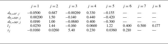
 \begin{align} {C_{d}^{\theta _i}} &= \underbrace {\frac {{24}}{{Re}}{g_{{\theta _i}}}(\beta )}_{\textrm {Stokes flow}}\bigl(\underbrace {\mathop {\textrm {1 + 0}.\textrm {1}{\textrm {5}{Re}^{\textrm {0}.\textrm {687}}}}\limits _{} }_{\scriptstyle \textrm {Empirical expression}\atop \scriptstyle \textrm {for sphere}}\nonumber\\&\quad + \underbrace {\mathop {}\limits _{} {d_{{\theta _i},1}}\left ( {\log \beta } \right )R{{e}^{{d_{{\theta _i},2}} + {d_{{\theta _i},3}}\log \beta }}\mathop {}\limits _{} }_{{\textrm {Shape correction for high }}Re} \bigr)\underbrace {\bigl(\mathop {}\limits _{} {d_{{\theta _i},4}}\sqrt N + {d_{{\theta _i},5}}H(N) + 1 \mathop {}\limits _{} \bigr)}_{\textrm {Magnetic field effect}} \end{align}
This expression consists of four components: the drag coefficient in the Stokes flow, the empirical-Reynolds-number correction for flows past a sphere, the shape and Reynolds-number corrections resulting from geometric characteristics, and the influence of the magnetic field. The expressions for the shape functions
 ${g_{{\theta _i}}} ( \beta )$
are provided in the Appendix C, and the values of
 $d_{{\theta _i}}$
are specified in table 8. Additionally, a comparison between the values calculated using expressions in (3.1) (
 $C_{d,\textit{Expression}}$
) and those obtained through simulations (
 $C_{d,\textit{Simulation}}$
) is presented in figure 20, which shows good agreement.
Validation of the drag coefficient expressions. (a) Drag coefficient expressions compared with simulation data, covering a total of 965 cases. (b) Relative error
 $( {( {{C_{d,\textit{Simulation}}} - {C_{d,\textit{Expression}}}} )\textrm {/}{C_{d,\textit{Expression}}}} )$
in different cases.

3.2.2. Lift expression
In the steady state regime, the lift force primarily acts in the
 $y$
-direction. Therefore, the lift coefficients
 $C_l$
in this section represent the lift coefficients in the
 $y$
-direction. The lift expression provided in (1.3) for arbitrary
 $\theta$
without a magnetic field can also be derived through the synthesis and decomposition of forces in the Stokes flow, illustrated in figure 18. When extending (1.3) from the Stokes flow to higher Reynolds numbers, there is a phase shift and a variation in the maximum value, as shown in figure 21(a). These effects can be corrected using the modified form in (1.5). The introduction of a magnetic field intensifies both the phase shift and the variation in the maximum value, necessitating further corrections. A dedicated explanation of the physical mechanism behind this phase shift is provided in Appendix B. The expression of the corrected form of lift expression is given as
 \begin{equation} {C_{l,\theta }} = {C_{l,\textit{max}}}\left ( {\textit{Re},\beta ,N} \right )\underbrace {\sin \left ( {2{\psi _l}\left ( {\textit{Re},\beta ,N,\theta } \right )} \right )}_{\scriptstyle \textrm {The synthesis and decomposition}\atop \scriptstyle \textrm {of forces in Stokes flow}}\!\!\!. \end{equation}
Lift coefficients at
 $\beta = 2$
,
 $Re=200$
with different inclination angles and magnetic fields. (a) The phase shift of the sine relationship with
 $C_l$
and
 $\theta$
. (b) The linear relationship with
 $C_l$
and
 $\sqrt N$
when
 $N \geqslant 1$
.

Initially, the correction for the phase shift in (3.6) affected by a streamwise magnetic field is based on the form in (1.5) without a magnetic field. The phase angle
 $\psi _{l}$
is expressed as
 \begin{equation} {\psi _{l}} \left ( {{\mathop {\textit{Re}}\nolimits } ,N,\beta ,\theta } \right ) = \frac {\pi }{2}{\left ( {\frac {\theta }{{{\pi \mathord {\left / {\vphantom {\pi 2}} \right . } 2}}}} \right )^{\!1 + {l_{6}}{{\left ( {\log \beta } \right )}^{{l_{7}}}}{{\left ( {\log Ha} \right )}^{{l_{8}}}}}} \end{equation}
where
 $Ha$
represents the Hartmann number and is defined as
 $Ha = \sqrt {N{\mathop {\textit{Re}}\nolimits } }$
. Subsequently, to determine the lift coefficient values at different inclination angles
 $\theta$
, expressions for the maximum value of the lift coefficient
 $C_{l,max}$
mentioned in (3.5) must be derived. It is evident that
 ${C_{l}} \sim \sqrt N$
also holds for
 $C_{l}$
at a constant
 $\theta$
, as shown in figure 21(b). This relationship can be analogously derived from the relationship
 ${C_{d}} \sim \sqrt N$
in the transverse magnetic field as established by Pan et al. (Reference Pan, Zhang and Ni2019). Due to the phase shift induced by higher Reynolds numbers and interaction parameters, the inclination angle
 $\theta$
corresponding to
 $C_{l,\textit{max}}$
shifts from
 $45^\circ$
to a larger
 $\theta$
. In figure 21(a), empirical testing determines that the lift coefficient at
 $\theta = 60^\circ$
is adopted as
 $C_{l,\textit{max}}$
. The lift force of an inclined spheroid can be interpreted as the drag projections caused by the incoming flow components along the spheroid’s major axis and its perpendicular axis, relative to the flow direction. This concept is illustrated in figure 18. Consequently, the expression for
 $C_{l,\textit{max}}$
shares a similar form with
 $C_{d}^\theta$
. By combining the effects of these two components through superposition, the expression for
 $C_{l,\textit{max}}$
is presented in (3.7) as
 \begin{equation} {C_{l,\textit{max} }}\!\left ( {\textit{Re},N,\beta } \right ) = \underbrace {\frac {{24}}{{\textit{Re}}}k(\beta )}_{\textrm {Stokes flow}}(\!{\kern-2pt}\underbrace{\mathop{\textrm{1 + 0}.\textrm {1}{\textrm {5}\textit{Re}^{\textrm {0}.\textrm {687}}}}\limits _{} }_{\scriptstyle \textrm {Empirical expression}\atop \scriptstyle \textrm {sphere}} + \underbrace {\mathop {}\limits _{} {l_1}\left ( {\log \beta } \right )\textrm {R}{\textrm {e}^{{l_2} + {l_3}\log \beta }}\mathop {}\limits _{} }_{\textrm {Shape correction}})\underbrace {(\mathop {}\limits _{} {l_4}\sqrt N + {l_5}\mathop {}\limits _{} )}_{\textrm {Magnetic field effect}}\!\!\! .\end{equation}
It consists of four components: the lift coefficient at
 $\theta ={60^ \circ }$
in Stokes flow, the empirical-Reynolds-number corrections for flows past a sphere, the shape and Reynolds-number corrections due to geometric specificity, and the impact of the magnetic field. The expression for the shape function
 $k(\beta )$
is provided in Appendix C, and the values of
 $l_i$
are specified in table 8. As
 $N$
approaches 0 and
 $\beta$
approaches 1,
 $C_{l}$
converges to 0. Similarly, a comparison of the values calculated using expressions in (3.5) (
 $C_{l,\textit{Expression}}$
) and those obtained through simulations (
 $C_{l,\textit{Simulation}}$
) is presented in figure 22, which shows good agreement.
Validation of the lift coefficient expressions. (a) Lift coefficient expressions compared with simulation data, covering a total of 992 cases. (b) Relative error
 $( {( {{C_{l,\textit{Simulation}}} - {C_{l,\textit{Expression}}}} )\textrm {/}{C_{l,\textit{Expression}}}} )$
in different cases.

3.2.3. Torque expression
In the steady state regime, the pitching torque primarily acts in the
 $z$
-direction. Therefore, the torque coefficients
 $C_t$
in this section represent the torque coefficients in the
 $z$
-direction. The torque coefficient
 $C_{t}$
versus
 $\sin 2\theta$
for an arbitrary
 $\theta$
without a magnetic field can be derived through the superposition of potential flow functions in Wu (Reference Wu1983). However, extending to higher Reynolds numbers requires correction for the phase shift and the variation in the maximum value, as shown in figure 23(a). These effects can be corrected using the modified form in (1.6). Additionally, applying a streamwise magnetic field intensifies this phenomenon. A dedicated explanation of the physical mechanism behind this phase shift is provided in Appendix B. Therefore, the expression of the corrected form of torque correlation is given as
 \begin{equation} {C_{t,\theta }}= {C_{t,\textit{max}}}\left ( {{\mathop {\textit{Re}}\nolimits } ,N,\beta } \right )\sin \left ( {2{\psi _{t}} \left ( {{\mathop {\textit{Re}}\nolimits } ,N,\beta ,\theta } \right )} \right )\!. \end{equation}
Torque coefficients at
 $\beta = 2$
,
 $Re=200$
with different inclination angles and magnetic fields. (a) The phase shift of the sine relationship with
 $C_t$
and
 $\theta$
. (b) The linear relationship with
 $C_t$
and
 $\sqrt N$
when
 $N \geqslant 1$
.

Initially, the correction for the phase shift affected by a streamwise magnetic field is based on the expression without a magnetic field as
 \begin{equation} {\psi _{t}} \left ( {{\mathop {\textit{Re}}\nolimits } ,N,\beta ,\theta } \right ) = \frac {\pi }{2}{\left ( {\frac {\theta }{{{\pi \mathord {\left / {\vphantom {\pi 2}} \right . } 2}}}} \right )^{1 + {t_{4}}{{\left ( {\log \beta } \right )}^{{t_{5}}}}{{\left ( {\log Ha} \right )}^{{t_{6}}}}}}. \end{equation}
Subsequently, to determine the torque coefficient values at different inclination angles
 $\theta$
, expressions for the maximum value of the torque coefficient
 $C_{t,max}$
mentioned in (3.8) must be derived. It is evident that
 ${C_{t}} \sim \sqrt N$
also holds for
 $C_{t}$
at a constant
 $\theta$
, as shown in figure 23(b). This arises from the fact that the pitching torque can be derived through the cross product of the lift and drag forces by their respective force arms. Coupling the influences of these two aspects through superposition, the expression for
 $C_{t,max}$
is presented in the form with reference to that without a magnetic field as
 \begin{equation} {C_{t,\textit{max}}}\left ( {{\mathop {\textit{Re}}\nolimits } ,N,\beta } \right ) = - \frac {{\log \beta }}{{{{{\mathop {\textit{Re}}\nolimits } }^{{t_{1}}}}}}( {{t_{2}}\sqrt N + {t_{3}}} ). \end{equation}
The values of
 $t_i$
are specified in table 8. As
 $N$
approaches 0 and
 $\beta$
approaches 1,
 $C_{t}$
converges to 0. Likewise, a comparison of the values calculated using (3.8) (
 $C_{t,\textit{Expression}}$
) and those obtained through simulations (
 $C_{t,\textit{Simulation}}$
) is presented in figure 24, which shows good agreement.
Validation of the torque coefficient expressions. (a) Torque coefficient expressions compared with simulation data, covering a total of 992 cases. (b) Relative error
 $( {( {{C_{t,\textit{Simulation}}} - {C_{t,\textit{Expression}}}} )/{C_{t,\textit{Expression}}}} )$
in different cases.

4. Summary
This study employs three-dimensional simulations to analyse wake patterns and derives expressions for force and torque coefficients for flows past an insulated spheroid under the influence of a streamwise magnetic field. A total of 1150 cases are computed for various combinations, including Reynolds number
 $50 \leqslant \textit{Re} \leqslant 250$
, aspect ratio
 $1.5 \leqslant \beta \leqslant 6$
, inclination angle
 ${0^ \circ } \leqslant \theta \leqslant {90^ \circ }$
, and interaction parameter
 $0 \leqslant N \leqslant 10$
. Nine wake patterns characterised by steady/unsteady state, flow symmetry, closed/open separation lines for steady state and single/multiple frequency for unsteady state are identified. These patterns are governed by four dimensionless parameters: Re,
 $\beta$
,
 $\theta$
, and
 $N$
. Without a magnetic field, enhancing
 $\beta$
increases the SL flow (feed the vortex spiral pair of
 $S_1$
and
 $S_2$
), while decreases the FM and SM flows (flow around
 $L_2$
to feed
 $L_1$
), generating rich wake structures. With a streamwise magnetic field, a reversion phenomenon is observed, which describes the wake structure at a higher Reynolds number and a certain magnetic interaction parameter
 $N$
corresponds to a lower Re with a lower
 $N$
for the fixed
 $\beta$
and
 $\theta$
. In summary, the magnetic field (not strong enough) stabilises the flow, delays separation, and increases the threshold for unsteady states. The results of those nine wake patterns are summarised in three maps of regimes basing on the inclination angle.
The simulated data are used to derive expressions for the forces and torques acting on an inclined spheroid with a streamwise magnetic field, based on three physical criteria. These expressions include the drag coefficient derived from Stokes flow, linear relationships between
 $C_d$
,
 $C_{l}$
,
 $C_{t}$
, and
 $\sqrt {N}$
derived from an energy perspective for large values of
 $N$
, as well as relationships such as
 ${C_d} \sim {\sin ^2}\theta$
,
 ${C_{l}}, {C_{t}} \propto \sin 2\theta$
derived from the synthesis and decomposition of forces in Stokes flow and the superposition of potential and flow functions in irrotational flow. At higher Reynolds numbers and interaction parameter, the previously observed relationships between
 $C_d$
,
 $C_{l}$
, and
 $C_{t}$
with
 $\theta$
are disrupted, requiring correction. As
 $N$
approaches 0, the corrected expressions for
 $C_d$
converge to the values without a magnetic field. Furthermore, as the aspect ratio
 $\beta$
approaches 1, both
 $C_{l}$
and
 $C_{t}$
converge to 0, and the corrected expressions for
 $C_d$
approach the drag coefficient for flows past a sphere
 $C_{d,sphere}$
without a magnetic field. The comparisons of the values calculated using the force and torque expressions and those obtained through simulations show a good agreement.
Funding.
The authors gratefully acknowledge support from the National Key Research and Development Program of China (no. 2022YFE03130000), the National Natural Science Foundation of China (nos 12472260, U23B20110, 12388101), the Innovation Special Project of the Bureau of Major Science and Technology Programs by CAS (no. RCJJ-145-24-58), the Young Elite Scientists Sponsorship Program by CAST (no. 2022QNRC001).
Declaration of interests.
The authors report no conflict of interest.
Author contributions.
T.-T.L. and J.-H.P contributed equally to this work and should be considered co-first authors.
Appendix A. High aspect ratio wake behaviour expansion
To further support the hypothesis that increasing the aspect ratio
 $\beta$
causes the spheroid to exhibit wake features similar to those of a circular cylinder, we present a supplementary case at
 $\beta = 15$
,
 $\rm Re = 250$
,
 $N = 0$
and
 $\theta = 90^\circ$
. Although this case lies outside our primary study range, it serves as a meaningful intermediate state that bridges spheroidal and cylindrical geometries. Figure 25 illustrates the wake structures in both the
 $xoy$
and
 $xoz$
planes. The flow field clearly demonstrates characteristics of a classical Kármán vortex street, including alternating vortex shedding and symmetric vortex pair structures. This provides qualitative support for the convergence of spheroidal wake patterns toward those of circular cylinders at high
 $\beta$
.
To quantitatively assess this convergence, we introduce comparative definitions for the Reynolds and Strouhal numbers of both the spheroid and a circular cylinder. For the spheroid, the Reynolds number and Strouhal number are defined as
 \begin{equation}\textit{Re}_s = \frac {u_\infty {d}_s}{\nu }, \quad St_s = \frac {f_s {d}_s}{u_\infty }, \end{equation}
where
 ${d}_s$
and
 ${f}_s$
denote the short-axis diameter and the vortex shedding frequency of the spheroid, respectively. For the cylinder,
 ${d}_c$
and
 ${f}_c$
are the diameter and the vortex shedding frequency of the cylinder. We use
 ${d}_c = {d}_s$
to ensure a consistent Reynolds number, leading to:
 \begin{equation} \textit{Re}_c = \frac {u_\infty {d}_c}{\nu }, \quad St_c = \frac {f_c {d}_c}{u_\infty }. \end{equation}
Table 6 compares
 $St_s$
,
 $St_c$
and their relative deviation for several values of
 $\beta$
. It is evident that the deviation
 $\left |( {St_c - St_s})/{St_c} \right |$
diminishes as
 $\beta$
increases. For instance, at
 $\beta = 3$
, the deviation is 36.7 %, whereas at
 $\beta = 15$
, it drops significantly to 14.1 %. This trend quantitatively confirms that as the spheroid becomes more elongated, its vortex shedding behaviour progressively aligns with that of a cylinder.
Comparison of the Strouhal number of flow past an spheroid
 $St_s$
with the same corresponding Reynolds number of the flow past a cylinder
 $St_c$
.

The isosurfaces of
 $Q$
contours with
 $Q=0.5$
for
 $\beta = 15$
,
 $Re=250$
,
 $N = 0$
,
 $\theta = {90^\circ }$
: (a) in
 $xoy$
plane, (b) in
 $xoz$
plane.

Furthermore, it is well established that vortex shedding behind a circular cylinder ceases when
 $\rm Re$
falls below approximately 47 (Williamson Reference Williamson1996; Cantwell & Barkley Reference Cantwell and Barkley2010). For a spheroid with constant inflow velocity, the short-axis Reynolds number
 $\rm Re_s$
decreases with increasing
 $\beta$
and is expected to drop below this critical threshold at approximately
 $\beta = 160$
. Therefore, it can be postulated that the spheroid will eventually revert to a steady state pattern as
 $\beta$
continues to increase until reaching a critical value of approximately
 $\beta = 160$
.
Appendix B. Explanation of the non-monotonic behaviour of drag coefficient and the phase shift of lift and torque coefficients
Although (1.2) is derived under the assumptions of Stokes flow, it has been shown to remain effective for Reynolds numbers up to approximately 2000. Sanjeevi, Kuipers & Padding (Reference Sanjeevi, Kuipers and Padding2018) demonstrated that, at higher Reynolds numbers and varying incident angles, when a magnetic field is applied, both the pressure distribution and the streamlines in the wake region are changed. The streamlines attach more closely to the surface of the spheroid, and the recirculation bubble disappears at
 $\theta = 60^\circ$
, while it persists at
 $\theta = 90^\circ$
, as shown in figure 27. This indicates that the Lorentz force performs more significant work at
 $\theta = 60^\circ$
than at
 $\theta = 90^\circ$
, resulting in a higher drag coefficient
 $C_d$
at the former. This leads to a non-monotonic trend in
 $C_d$
as the magnetic field increases, as shown in figure 26(a).
Influence of high Reynolds number and magnetic field on drag, lift and torque coefficients at
 $\beta = 2$
. (a) Drag coefficient
 $C_d$
. (b) Lift coefficient
 $C_l$
. (c) Torque coefficient
 $C_t$
.

The pressure contours and streamlines projected in the
 $xoy$
plane with
 $\beta = 2$
.

However, the phase shift in the lift and torque coefficients, as shown in figures 21 and 23, becomes prominent under higher Reynolds numbers and interaction parameters
 $N$
. Similar phase shifts under high Reynolds numbers have been reported in previous studies (Zastawny et al. Reference Zastawny, Mallouppas, Zhao and Van Wachem2012; Sanjeevi & Padding Reference Sanjeevi and Padding2017; Fröhlich et al. Reference Fröhlich, Meinke and Schröder2020). Equation (1.3), describing the lift coefficient
 $C_l$
, is derived under the assumption of Stokes flow, where inertial effects are negligible. As the Reynolds number and magnetic field increase, the deviation from this assumption becomes more pronounced, which leads to the phase shift and a variation in the maximum value of
 $C_l$
. For a fixed aspect ratio
 $\beta$
, smaller inclination angles (
 $\theta \leqslant {30^\circ }$
) exhibit boundary-layer separation and form a recirculation bubble at larger
 $\textit{Re}$
than larger inclination angles (
 $\theta \geq {45^\circ }$
), as shown in figure 27. Additionally, smaller inclination angles are less likely to produce a recirculation bubble, indicating weaker inertial effects. Consequently, the lift coefficient
 $C_l$
increases more significantly at larger inclination angles than at smaller ones. This causes the inclination angle corresponding to the maximum lift coefficient,
 $C_{l,\textit{max}}$
, to shift from
 $45^\circ$
to a larger
 $\theta$
, as shown in figure 26(b).
Equation (1.4), which defines the torque coefficient
 $C_{t}$
, is based on a superposition of potential flow solutions and assumes an inviscid, irrotational and incompressible flow governed by Laplace’s equation. However, the flow in our study is both viscous and affected by a streamwise magnetic field, leading to deviations from the theoretical predictions. Without a magnetic field, smaller inclination angles are less likely to produce a recirculation bubble, suggesting stronger viscous effects. This causes a slight shift in the inclination angle corresponding to
 $C_{t,\textit{max}}$
from
 $45^\circ$
to a smaller
 $\theta$
, as shown in figure 26(c). When applying a magnetic field, as demonstrated by Pan et al. (Reference Pan, Zhang and Ni2018), the flow exhibits characteristics similar to those of lower-Reynolds-number flows. The Lorentz force, particularly the Maxwell stresses, acts similarly to distributed viscous stresses. Thus, increasing the magnetic field enhances the viscous effect, causing further deviations from the predictions of potential flow theory. This effect is especially pronounced at larger inclination angles, where the recirculation bubble disappears (see figure 27) and the Lorentz force performs more work on the flow. As a result, the angle corresponding to
 $C_{t,\textit{max}}$
shifts from
 $45^\circ$
to a larger
 $\theta$
, as shown in figure 26(c).
Appendix C. The parameters and shape functions for force and torque coefficients expressions
Following Jeffery (Reference Jeffery1922), the drag coefficients
 $C_{d,{\textit{Stokes}}}^{{0}^ \circ }$
and
 $C_{d,{\textit{Stokes}}}^{{90}^ \circ }$
can be summarised as
 $${C_{d,{\textit{Stokes}}}^{{0}^ \circ }}= \frac {{64}}{{{\mathop {\textit{Re}}\nolimits } }}\frac {{{\beta ^{\frac {2}{3}}}}}{{{\chi _0} + {\beta ^2}{\gamma _0}}} = \frac {{24}}{{{\mathop {\textit{Re}}\nolimits } }}{g_{{0^ \circ }}}\left ( \beta \right )\! ,$$
 $${C_{d,{\textit{Stokes}}}^{{90}^ \circ }} = \frac {{64}}{{{\mathop {\textit{Re}}\nolimits } }}\frac {{{\beta ^{\frac {2}{3}}}}}{{{\chi _0} + {\alpha _0}}} = \frac {{24}}{{{\mathop {\textit{Re}}\nolimits } }}{g_{{{90}^ \circ }}}\left ( \beta \right )\!.$$
Analytical shape coefficients for spheroids with
 $\beta \gt 1$
.

Parameters for drag coefficient
 $C_d$
, lift coefficient
 $C_{l}$
and torque coefficient
 $C_{t}$
expressions.

According to the orientation-dependent drag expression for Stokes flow in (1.2),
 $C_{d,{\textit{Stokes}}}^{{60}^ \circ }$
can be defined by
 \begin{equation} \begin{aligned} {C_{d,{\textit{Stokes}}}^{{60}^ \circ }} & = {C_{d,{\textit{Stokes}}}^{{0}^ \circ }} + \big( {C_{d,{\textit{Stokes}}^{{90}^ \circ }}} \big){\sin ^2}{60^ \circ } \\ & = \frac {{24}}{{{\mathop {\textit{Re}}\nolimits } }}\big[{{g_{{0^\circ }}}\left ( \beta \right ) + \left ( {{g_{{{90}^\circ }}}\left ( \beta \right ) - {g_{{0^\circ }}}\left ( \beta \right )} \right ){{\sin }^2}{{60}^ \circ }} \big] = \frac {{24}}{{{\mathop {\textit{Re}}\nolimits } }}{g_{{{60}^\circ }}}\left ( \beta \right )\!. \end{aligned} \end{equation}
According to the orientation-dependent lift expression for Stokes flow in (1.3),
 $C_{l,{\textit{Stokes}}}^{{60}^ \circ }$
can be defined by
 \begin{equation} \begin{aligned} {C_{6,{\textit{Stokes}}}^{{60}^ \circ }} & = \big({{C_{d,{\textit{Stokes}}}^{{90}^ \circ }} - {C_{d,{\textit{Stokes}}}^{{0}^ \circ }}} \big)\sin {60^ \circ }\cos {60^ \circ }\\ & = \frac {{24}}{{{\mathop {\textit{Re}}\nolimits } }}\left [ {\left ( {{g_{{{90}^\circ }}}\left ( \beta \right ) - {g_{{0^\circ }}}\left ( \beta \right )} \right )\sin {{60}^ \circ }\cos {{60}^ \circ }} \right ] = \frac {{24}}{{{\mathop {\textit{Re}}\nolimits } }}{k}\left ( \beta \right )\!. \end{aligned} \end{equation}
Therefore, shape functions
 ${g_{{0^\circ }}} ( \beta )$
,
 ${g_{{{90}^\circ }}} ( \beta )$
,
 ${g_{{{60}^\circ }}} ( \beta )$
and
 $k ( \beta )$
can be defined by
 $${g_{{0^\circ }}}\left ( \beta \right ) = \frac {8}{3}\frac {{{\beta ^{\frac {2}{3}}}}}{{{\chi _0} + {\beta ^2}{\gamma _0}}},$$
 $${g_{{{90}^\circ }}}\left ( \beta \right ) = \frac {8}{3}\frac {{{\beta ^{\frac {2}{3}}}}}{{{\chi _0} + {\alpha _0}}},$$
 $${g_{{{60}^ \circ }}}\left ( \beta \right ) = {g_{{0^ \circ }}}\left ( \beta \right ) + \left ( {{g_{{{90}^ \circ }}}\left ( \beta \right ) - {g_{{0^ \circ }}}\left ( \beta \right )} \right ){\sin ^2}{{60}^ \circ },$$
 $$k\left ( \beta \right ) = \left ( {{g_{{{90}^ \circ }}}\left ( \beta \right ) - {g_{{0^ \circ }}}\left ( \beta \right )} \right )\sin {{60}^ \circ } \cos {{60}^ \circ }.$$
The shape parameters
 ${\chi _0}$
,
 ${\gamma _0}$
and
 ${\alpha _0}$
, initially proposed by Oberbeck (Reference Oberbeck1876) and subsequently summarised by Hölzer & Sommerfeld (Reference Hölzer and Sommerfeld2008), are provided in table 7. Comparable expressions are also available in Happel & Brenner (Reference Happel and Brenner2012). The fitting parameters for the drag expressions
 $d_{{\theta _i},j}$
, the lift expression
 $l_j$
, and the torque expression
 $t_j$
are summarised in table 8.