
1. Introduction
Membrane filtration is a process used for the clarification, purification and separation of fluid mixtures (Noble & Stern Reference Noble and Stern1995). This field has many important applications from filtering of blood to purifying water and air (van Reis & Zydney Reference van Reis and Zydney2007; Lee, Arnot & Mattia Reference Lee, Arnot and Mattia2011). In a typical filtration system, a mixture of fluid and contaminant particles is passed through a porous membrane; the fluid passes through while the particles are retained, either on the surface of the membrane or within the membrane structure.
Filtration membranes can be divided broadly into two main types: fibre-based membranes comprise a random network of fibres, and membrane surfaces are manufactured with pores. While fibre-based membranes have historically been easier to manufacture, they come with several drawbacks. For example, there is minimal control of their pore structure and they have a large environmental footprint since the fibres clog and have to be discarded, increasing waste to landfill. As such, the second type of manufactured membranes, which has the benefit of a controlled pore structure and the potential to be cleaned and reused, is often the preferable choice. Furthermore, new techniques are emerging to manufacture such membranes more easily (Smart Separations Ltd 2020).
As the unwanted particles are filtered out of the fluid mixture, the membrane blocks over time. There are two main blocking mechanisms: caking is the build-up of large particles on the surface of the membrane, and internal blocking is the clogging inside the actual pore. Blocking is inevitable in filtration. It affects the flux of fluid through the membrane, and consequently the efficiency of a filter is strongly coupled to any blocking.
The blocking of filters motivates the study of filtration devices, with the goal of finding the optimal filter design, i.e. the design that maximises flux through the filter and minimises the effect of blocking. Filtration devices can be classified by the direction of flow: fluid mixtures are passed through filtration membranes with the flow either perpendicular to the membrane surface in what is called dead-end flow, or parallel to the surface in cross-flow (Noble & Stern Reference Noble and Stern1995).
When using a filter in dead-end flow, all of the components of the fluid mixture are either passed through or retained by the membrane. While dead-end flow is simple to use, the technique is unsuitable for processing high volumes as the normal flow results in cake layers building up quickly. In cross-flow devices, the fluid mixture is passed parallel to the membrane surface; the predominant flow direction is parallel to the membrane with some of the flow travelling into the membrane. The fluid mixture is therefore processed slower through a cross-flow device than a dead-end flow device. The advantage of the predominant flow direction being parallel is that the flow continuously ‘washes’ the membrane surface and thereby inhibits cake build-up. Thus, although slow, cross-flow devices can be used to process higher volumes of fluid than direct flow. The disadvantage of this method is that the process requires recirculation of the fluid, and is consequently more complex and energy consuming.
Direct-flow filtration devices consist of cross-flow membranes with capped ends. This design therefore also benefits from reduced cake build-up. The capped ends act to drive the fluid mixture through the membrane thereby also utilising the dead-end technology resulting in a more economical and more energy efficient filtration device than cross-flow devices. Typically, direct-flow devices comprise vertically stacked filtration membranes.
There have been numerous studies into the mathematical modelling of vertically stacked direct-flow filtration devices (Herterich et al. Reference Herterich, Xu, Field, Vella and Griffiths2017; Wang, Mondal & Griffiths Reference Wang, Mondal and Griffiths2017; Xu, Pearce & Field Reference Xu, Pearce and Field2017). Of particular relevance to this paper is Herterich et al. (Reference Herterich, Xu, Field, Vella and Griffiths2017), who developed a mathematical model for flow through a direct-flow device comprising a system of stacked cylinders, where the porous cylinder walls provide the parallel membrane surfaces for cross-flow. A key observation was that when the membranes were stacked too closely or too sparsely, the total flux through the device was reduced and hence there was an optimal stacking distance.
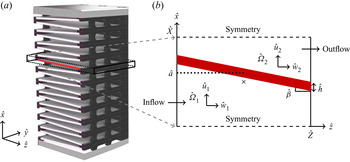
In this paper we will examine how the design set-up affects the flow through a direct-flow device with angled membranes. An industrial example and motivation for this is the direct-flow device designed by Smart Separations Ltd (2020). A schematic for this filter is shown in figure 1(a). There are similarities between a direct-flow device with angled membranes and a pleated filtration membrane. The main distinction between the two is that fluid can travel through the full porous pleated membrane structure, whereas direct-flow devices comprise dead ends (see figure 1) through which the flow cannot travel. The dead ends change the flow structure within the filter. There has been research studying the flow through pleated membranes to determine the optimal pleat density in such a membrane (Chen, Pui & Liu Reference Chen, Pui and Liu1995; Rebaï et al. Reference Rebaï, Prat, Meireles, Schmitz and Baclet2010). Additionally, previous studies have examined the effect of the geometry on the pressure drop achieved across a single pleat for a given flux (Caesar & Schroth Reference Caesar and Schroth2002; Saleh, Tafreshi & Pourdeyhimi Reference Saleh, Tafreshi and Pourdeyhimi2016; Théron, Joubert & Le Coq Reference Théron, Joubert and Le Coq2017).
Schematic of the concertinaed filtration device. Panel (a) shows the full three-dimensional device; reproduced from Smart Separations Ltd (2020) with permission. Panel (b) depicts the two-dimensional domain of a single filtration module; the centre of the domain  $({\hat {x}},{\hat {z}}) = ({\hat {X}}/2, {\hat {Z}}/2)$ is indicated by a cross.

Recent relevant studies by Sanaei et al. (Reference Sanaei, Richardson, Witelski and Cummings2016) and Sun et al. (Reference Sun, Sanaei, Kondic and Cummings2020) model the flow and blocking mechanisms in pleated devices, adopting the assumption of Darcy flow throughout the whole domain composed of rectangular pleats. The focus of these works was to find the filter design that optimised the lifetime of the filter accounting for transient blocking dynamics. Earlier work by King & Please (Reference King and Please1996) also models the flow through a pleated filtration membrane. The authors account for Stokes flow between the membranes driven by a prescribed flux through rectangular pleats with porous walls and ends, with a focus on the shape of cake build-up along the membrane surface.
The distinction between previous work on examining the transient flow through a pleated device and the work presented here is that we focus specifically on understanding how filters can be designed to optimise filtration, and on exploring how the optimal design changes as operating parameters vary. This is particularly useful for direct-flow devices since their geometry can be precisely controlled through modern manufacturing techniques. Specifically, we examine how the angle and position of the membrane affect the steady flow driven by a prescribed pressure drop. The model we develop here is relevant for new filters over time scales before blocking becomes important (i.e. months), and for filters where blocking is not relevant. An example of the latter is Smart Separation Ltd.'s novel virus filter, which works through neutralisation of the viruses without changing the physical properties of the filtration system through blocking (Smart Separations Ltd 2020).
1.1. Problem statement
In this paper, we present a comprehensive study of a direct-flow device with angled membranes. The angled membranes increase the membrane surface area in a concertinaed filtration device, as shown in figure 1(a). Our main objective is to determine the optimal set-up to maximise the flux for a given pressure drop.
We develop a mathematical model of flow through a filtration device with openings through which the fluid is introduced and removed, closed ends, and porous membranes. The concertina structure comprises repeated single modules, as shown in figure 1(a). The flow is driven by a pressure gradient, and we study how the optimal flow depends on the system parameters defining a single repeated module.
We build on the modelling approach used by Herterich et al. (Reference Herterich, Xu, Field, Vella and Griffiths2017), who considered the similar problem of an applied flux through horizontal walls, to study the design of an angled membrane module that maximises the flux for a given applied pressure difference. The structure of this paper is as follows. In § 2 we formulate the coupled lubrication flow problem through a single repeated module. In § 3, we consider an infinitely thin membrane with a specified angle and permeance. The permeance is defined as the inverse of the resistance and determines the ease in which fluid may pass through the membrane. We determine the membrane position within the module that results in the maximum flux. We analyse two parameter regimes: the first for a slightly angled membrane in § 3.1, and the second for an arbitrarily angled membrane in § 3.2. In § 4, we determine the optimal angle and position associated with the maximum flux through a membrane of specified thickness and permeance. We first consider vanishingly thin membranes and study the role of permeance in § 4.1. We then extend our study to membranes of finite thickness in § 4.2. In § 5 we discuss the implications and conclusions of our work, as well as avenues of future work.
2. Model development
We model the flow through a single repeated module of the filtration device shown in figure 1(a). The system geometry is such that the vertical length  ${\hat {X}}$ is significantly smaller than the horizontal height
 ${\hat {Z}}$ and lateral depth
 ${\hat {Y}}$ (see table 1). We assume no flow in the
 $\hat {y}$-direction and therefore focus our attention to the two-dimensional domain in
 $({\hat {x}},{\hat {z}})$-space depicted in figure 1(b). We denote dimensional and dimensionless quantities with and without hats, respectively. The position of the membrane is described by the upstream side of the membrane wall
 ${\hat {x}}={\hat {m}}({\hat {z}})$ given by
 \begin{equation} {\hat{m}}({\hat{z}}) = {\hat{a}} + \tfrac{1}{2}\left({\hat{Z}}\tan{\hat{\beta}} - {\hat{h}}\right) -{\hat{z}} \tan{\hat{\beta}}, \end{equation}
where  ${\hat {h}}$ is the membrane thickness, and
 ${\hat {\beta }}$ is the angle of the membrane; see figure 1(b). The midpoint of the membrane at
 $({\hat {x}},{\hat {z}})=({\hat {a}},{\hat {Z}}/2)$ is specified by the parameter
 $\hat {a}$, which is used to prescribe the distance between the centres of the membranes in neighbouring modules. In the specific case that the midpoint of the membrane coincides with the midpoint of the domain, i.e.
 ${\hat {a}} = {\hat {X}}/2$, the membranes will be equally spaced.


The flow domain comprises two subdomains
 \begin{gather} {\hat{\varOmega}}_1 = \{ {\hat{x}}\in[0,{\hat{m}}({\hat{z}})],\ {\hat{z}}\in[0,{\hat{Z}}]\}, \end{gather}
 \begin{gather}{\hat{\varOmega}}_{2} = \{ {\hat{x}} \in [{\hat{m}}({\hat{z}})+{\hat{h}}, {\hat{X}}],\ {\hat{z}}\in[0,{\hat{Z}}]\}. \end{gather}
Note that, while  ${\hat {X}}$ and
 ${\hat {Z}}$ are specified constants, the membrane length
 ${\hat {L}}$ is coupled to the prescribed angle
 ${\hat {\beta }}$ and horizontal height
 ${\hat {Z}}$ via
 ${\hat {L}}= {\hat {Z}}/\cos {\hat {\beta }}$. In this paper, the angle
 ${\hat {\beta }}$ will constitute a key experimental parameter that can be varied. Moreover, without loss of generality, we consider
 ${\hat {\beta }} > 0$ and note that neighbouring modules have
 ${\hat {\beta }} < 0$ with the subdomains switched for symmetric flux, as can be seen in figure 1(a).
The flow enters  ${\hat {\varOmega }}_1$ at
 ${\hat {z}}=0$ with constant inlet pressure
 ${\hat {p}}_{{in}}$, and exits
 ${\hat {\varOmega }}_2$ at
 ${\hat {z}}={\hat {Z}}$ with constant outlet pressure
 ${\hat {p}}_{{out}}$. The pressure difference
 $(\kern0.08em {\hat {p}}_{{in}}-{\hat {p}}_{{out}})>0$ drives the flow through the porous membrane, and a particular quantity of interest is the flux through the domain.
2.1. Governing equations
The ratio between the vertical and horizontal domain lengths is  $\epsilon = {\hat {X}} /{\hat {Z}}$. Using the parameter values given in table 1, we find that
 $\epsilon \ll 1$. Moreover, the values in table 1 yield a small reduced Reynolds number
 $\epsilon ^2Re =\epsilon ^2\hat {\rho }\hat {W}_0 {\hat {Z}}/{\hat {\mu }}$. We therefore use the Stokes flow equations to describe the flow in
 $\hat {\varOmega }_1$ and
 $\hat {\varOmega }_2$:
 \begin{gather} \hat{\mu} \hat{\nabla}^2 \hat{{\boldsymbol{u}}} - \hat{\boldsymbol\nabla} {\hat{p}} = 0, \end{gather}
 \begin{gather}\hat{\boldsymbol\nabla} \boldsymbol{\cdot} \hat{{\boldsymbol{u}}} = 0, \end{gather}
where  $\hat {{\boldsymbol {u}}}({\hat {x}},{\hat {z}})=({\hat {u}}({\hat {x}},{\hat {z}}),\hat {w}({\hat {x}},{\hat {z}}))$ is the velocity,
 ${\hat {p}}$ is the pressure and
 $\hat {\mu }$ is the constant fluid viscosity. We seek steady solutions in both subdomains denoting the variables in
 ${\hat {\varOmega }}_1$ by
 $({\hat {u}}_1,\hat {w}_1,{\hat {p}}_1)$ and those in
 ${\hat {\varOmega }}_{2}$ by
 $({\hat {u}}_{2},\hat {w}_{2},{\hat {p}}_{2})$.
As described above, the flow enters the domain along  ${\hat {z}}=0$ into
 ${\hat {\varOmega }}_1$, passes through the membrane at
 ${\hat {x}} ={\hat {m}}({\hat {z}})$ and exits along
 ${\hat {z}}={\hat {Z}}$ from
 ${\hat {\varOmega }}_{2}$, driven by a pressure gradient. The boundary conditions at the inlet and outlet are
 \begin{gather} {\hat{p}}_1 = {\hat{p}}_{{in}} \quad \mbox{at } {\hat{z}}=0,\quad {\hat{x}}\in[0,{\hat{m}}(0)], \end{gather}
 \begin{gather}{\hat{p}}_{2} = {\hat{p}}_{{out}} \quad \mbox{at } {\hat{z}}={\hat{Z}},\quad {\hat{x}}\in[{\hat{m}}({\hat{Z}})+{\hat{h}}, {\hat{X}}]. \end{gather}
There are closed ends at  ${\hat {z}}={\hat {Z}}$ in
 ${\hat {\varOmega }}_{1}$ and at
 ${\hat {z}}=0$ at
 ${\hat {\varOmega }}_{2}$ through which the flow cannot penetrate. The following boundary conditions enforce no penetration as well as no slip
 \begin{gather} \hat{{\boldsymbol{u}}}_1 = \textbf{0} \quad \mbox{at } {\hat{z}}={\hat{Z}},\quad {\hat{x}}\in[0,{\hat{m}}({\hat{Z}})], \end{gather}
 \begin{gather}\hat{{\boldsymbol{u}}}_{2} = \textbf{0} \quad \mbox{at } {\hat{z}}=0,\quad {\hat{x}}\in[{\hat{m}}(0)+{\hat{h}}, {\hat{X}}]. \end{gather}
Since the entire filter consists of a periodic array of modules, we impose symmetry conditions across  ${\hat {x}}=0$ and
 ${\hat {x}}={\hat {X}}$, yielding
 \begin{gather} {\hat{u}}_1 = 0, \quad \frac{{\partial} \hat{w}_1}{{\partial} {\hat{x}}} = 0 \quad \mbox{at } {\hat{x}}=0, \end{gather}
 \begin{gather}{\hat{u}}_{2} = 0, \quad \frac{{\partial} \hat{w}_{2}}{{\partial} {\hat{x}}} = 0 \quad \mbox{at } {\hat{x}}={\hat{X}}. \end{gather}
The normal flow through the filter is modelled as a porous flow (i.e. governed by the pressure difference and permeance). Thus, employing Darcy flow across the membrane provides the boundary condition for the velocity in  ${\hat {\varOmega }}_1$
 \begin{equation} \hat{{\boldsymbol{u}}}_1 \boldsymbol{\cdot} {\boldsymbol{n}} = {\hat{\kappa}} \left[{\hat{p}}_1({\hat{m}},{\hat{z}}) - {\hat{p}}_{2}({\hat{m}}+{\hat{h}},{\hat{z}})\right] \quad \mbox{at } {\hat{x}}={\hat{m}}({\hat{z}}), \end{equation}
where  ${\boldsymbol {n}}=(\cos {\hat {\beta }}, \sin {\hat {\beta }})$ is the unit normal vector to the membrane and
 ${\hat {\kappa }} = {\hat {k}}/\hat {\mu } {\hat {h}}$ is the membrane permeance, where
 ${\hat {k}}$ is the permeability of the membrane. Note that the flow resistance due to the membrane is
 ${\hat {R}} = 1/{\hat {\kappa }}$.
A flux balance through the membrane provides the corresponding boundary condition for the velocity in  ${\hat {\varOmega }}_{2}$
 \begin{equation} \hat{{\boldsymbol{u}}}_{1}|_{{\hat{x}}={\hat{m}}} = \hat{{\boldsymbol{u}}}_{2}|_{{\hat{x}}={\hat{m}}+{\hat{h}}}. \end{equation}
Finally, we need conditions at the permeable membrane layer. While Beavers & Joseph (Reference Beavers and Joseph1967) provide an appropriate tangential slip-flow boundary condition, Griffiths, Howell & Shipley (Reference Griffiths, Howell and Shipley2013) show that including slip does not have a significant effect on the flow. Hence, for simplicity, we impose no slip on both sides of the membrane
 \begin{gather} \hat{{\boldsymbol{u}}}_1 \boldsymbol{\cdot} {\boldsymbol{t}} = 0 \quad \mbox{at } {\hat{x}}={\hat{m}}({\hat{z}}), \end{gather}
 \begin{gather}\hat{{\boldsymbol{u}}}_{2}\boldsymbol{\cdot} {\boldsymbol{t}} = 0 \quad \mbox{at } {\hat{x}}={\hat{m}}({\hat{z}})+{\hat{h}}, \end{gather}
where  ${\boldsymbol {t}}=(-\sin {\hat {\beta }}, \cos {\hat {\beta }})$ is the unit tangent vector to the membrane.
2.2. Dimensionless model
We non-dimensionalise the system (2.3)–(2.9) by introducing the following scalings:
 \begin{equation} {\hat{z}} = {\hat{Z}} z, \quad {\hat{x}} = \epsilon {\hat{Z}} x, \quad {\hat{\beta}} = \epsilon \beta, \quad {\hat{u}} = \epsilon \hat{W}_0 u, \quad \hat{w} = \hat{W}_0 w, \quad {\hat{p}} = \frac{{\hat{\mu}} \hat{W}_0}{\epsilon^2 {\hat{Z}}} p+{\hat{p}}_{{out}}; \end{equation}
recalling that  $\epsilon = {\hat {X}}/{\hat {Z}}$. Note that the pressure difference is directly related to the velocity scale
 $W_0$ through (2.10a–f). Applying (2.10a–f) to (2.3) and taking the limit
 $\epsilon \to 0$ yields
 \begin{equation} p_x = 0, \quad w_{xx} - p_z = 0, \quad u_x + w_z = 0. \end{equation}
Hence, in both subdomains the lubrication equations govern the flow.
The leading-order position of the membrane (2.1) becomes
 \begin{equation} m(z) = a - \tfrac{1}{2}h + \beta\left(\tfrac{1}{2}-z\right), \end{equation}
where  $m={\hat {m}}/{\hat {X}}$,
 $a={\hat {a}}/{\hat {X}}$,
 $h={\hat {h}}/{\hat {X}}$ and the dimensionless membrane angle is
 $\beta \in [0,1]$. The corresponding dimensionless subdomains from (2.2) are given by
 \begin{gather} \varOmega_1 = \{ x\in[0,m(z)],\ z\in[0,1]\}, \end{gather}
 \begin{gather}\varOmega_{2} = \{ x \in [m(z)+h, 1],\ z\in[0,1]\}. \end{gather}
The dimensionless domain is identical to that shown in figure 1(b) with the hats removed and with the dimensionless vertical and horizontal lengths such that  $X=Z=1$. Recall that, while the domain size specified by
 $Z$ and
 $X$ is fixed, the membrane length varies with
 $\beta$.
Applying the scaling (2.10a–f) to the boundary conditions prescribed above, the pressure conditions (2.4) become
 \begin{gather} p_1 = 1 \quad \mbox{at } z=0,\quad x\in[0,m(0)], \end{gather}
 \begin{gather}p_{2} = 0 \quad \mbox{at } z=1,\quad x\in[m(1)+h, 1], \end{gather}
and the boundary conditions at the closed walls (2.5) become
 \begin{gather} w_1 = 0 \quad \mbox{at } z=1,\quad x\in[0,m(1)], \end{gather}
 \begin{gather}w_{2} = 0 \quad \mbox{at } z=0,\quad x\in[m(0)+h, 1]. \end{gather}
We note that information regarding the tangential velocity on the closed walls in (2.15) is lost since we are working in the lubrication regime. The dimensionless symmetry conditions from (2.6) are
 \begin{gather} u_1 = 0, \quad \frac{{\partial} w_1}{{\partial} x} = 0 \quad \mbox{at } x=0, \end{gather}
 \begin{gather}u_{2} = 0, \quad \frac{{\partial} w_{2}}{{\partial} x} = 0 \quad \mbox{at } x = 1. \end{gather}
We define the dimensionless permeance by  $\kappa = {\hat {\mu }} {\hat {\kappa }}/\epsilon ^3 {\hat {Z}}$, and the dimensionless permeability by
 $k = {\hat {k}}/\epsilon ^3 {\hat {Z}} {\hat {X}}$. With these definitions, the dimensionless permeance is
 $\kappa = k/h$. The Darcy flow condition through the membrane (2.7) becomes
 \begin{equation} u_1 =\kappa [\kern0.08em p_1(m,z) - p_{2}(m(z)+h,z)] \quad \mbox{at } x=m(z), \end{equation}
where the dimensionless membrane resistance is  $R=1/\kappa$. The flux-balance boundary condition across the membrane (2.8) becomes
 \begin{equation} u_{1}|_{x=m} = u_{2}|_{x=m+h}. \end{equation}
Finally, the dimensionless no-slip condition (2.9), exploiting the small angle of the membrane, is
 \begin{gather} w_1 = 0 \quad \mbox{at } x=m(z), \end{gather}
 \begin{gather}w_{2} = 0 \quad \mbox{at } x=m(z)+h. \end{gather}
2.3. Model reduction
Since  $p_1=p_1(z)$ and
 $p_2=p_2(z)$ from the momentum equation in the
 $x$-direction (2.11a), we can reduce the full problem (2.11)–(2.19) to modified Reynolds equations. Since we have two coupled domains, we derive two coupled second-order ordinary differential equations (ODEs) for the pressure; one ODE for each subdomain. The details are as follows.
In the region  $\varOmega _1$ we solve the momentum equation in the
 $z$-direction (2.11b) and the continuity equation (2.11c) with the symmetry and no-slip boundary conditions (2.16a) and (2.19a) to find the following relationships between the velocities and the pressure:
 \begin{gather} u_1 = \tfrac{1}{2}x\left[(\kern0.08em p_1' m^2)' - \tfrac{1}{3}x^2 p_{1}''\right], \end{gather}
 \begin{gather}w_1 = \tfrac{1}{2}\kern0.08em p_1' (x^2 - m^2), \end{gather}
where  $'$ denotes differentiation with respect to
 $z$ and recalling that
 $m=m(z)$ given in (2.12). We derive an equation for the pressure in
 $\varOmega _1$ by applying the Darcy flow boundary condition at the membrane (2.17)
 \begin{equation} \tfrac{1}{3}\left(\kern0.08em p_1'm^3 \right)' = \kappa\left(\kern0.08em p_1 - p_{2}\right). \end{equation}
The inlet pressure and closed end at  $z=1$ from (2.14a) and (2.15a) provide the two necessary boundary conditions for the pressure in
 $\varOmega _1$
 \begin{gather} p_1 = 1 \quad \mbox{at } z=0, \end{gather}
 \begin{gather}p_1' = 0 \quad \mbox{at } z=1. \end{gather}
Similarly, in  $\varOmega _{2}$, we solve the momentum (in the
 $z$-direction) and continuity equations (2.11b) and (2.11c) using the symmetry and no-slip boundary conditions (2.16b) and (2.19b) to derive
 \begin{gather} u_{2} = \tfrac{1}{2}(x-1)\left[\left(\kern0.08em p_2' (m+h-1)^2 \right)'- \tfrac{1}{3}(x-1)^2 p_{2}''\right], \end{gather}
 \begin{gather}w_{2} = \tfrac{1}{2} p_{2}' \left[ (x-1)^2 - (m+h-1)^2\right]. \end{gather}
The flux-balance boundary condition across the membrane (2.18) provides an equation for the pressure in  $\varOmega _2$
 \begin{equation} \tfrac{1}{3}\left[p_{2}'(m+h-1)^3 \right]' = \kappa\left(\kern0.08em p_1 - p_{2}\right). \end{equation}
The governing equation (2.24) is coupled to the following boundary conditions, which arise from the outlet pressure (2.14b) and closed end at  $z=0$ (2.15b):
 \begin{gather} p_{2} = 0 \quad \mbox{at } z=1, \end{gather}
 \begin{gather}p_{2}' = 0 \quad \mbox{at } z=0. \end{gather}
Thus, the problem is reduced to solving (2.21) and (2.22) for  $p_1$ in
 $\varOmega _1$ and (2.24) and (2.25) for
 $p_{2}$ in
 $\varOmega _{2}$. The parameters in the reduced system are the membrane permeance
 $\kappa$, the membrane thickness
 $h$ and the position of the membrane described by
 $a$ and
 $\beta$ in (2.12).
Our goal is to understand how to maximise the flux through the filter for an applied pressure difference across the filter. As such, it is helpful to define the dimensionless flux through the system, calculated at the inlet  $z=0$ as follows:
 \begin{equation} Q = \int_{0}^m w_1|_{z=0}\,{\textrm{d}x} ={-}\tfrac{1}{3} \left(\kern0.08em p_1'm^3\right) |_{z=0}. \end{equation}
The system parameters are  $a$,
 $\beta$,
 $\kappa$ and
 $h$; our goal is therefore to find the system set-up that maximises
 $Q(a,\beta ,\kappa ,h)$. We note that the analysis of this system is much clearer in the limit of small
 $h$. Moreover, this limit is a regular perturbation and a finite
 $h$ will only slightly change the quantitative results. We consequently consider the case
 $h = 0$ in § 3. However, as is realistic for the physical problem, we examine the quantitative changes that arise from accounting for
 $h>0$ in § 4.
3. The effect of angling the membrane
In this section, we seek to understand the effect of the membrane angle on the flux through the device. We consider a set-up in which we prescribe the membrane permeance  $\kappa$ and thickness
 $h$, and study the dependency of the maximum flux achievable and the associated membrane position on the membrane angle. We consider the regular limit of a thin membrane, taking
 $h=0$. Taking this limit greatly simplifies the analysis, and, as previously mentioned, the results we obtain are qualitatively consistent for
 $h\neq 0$.
In § 3.1, we first explore the limit of a slightly angled membrane within the dimensionless domain, corresponding to  $\beta \ll 1$. Recall that
 ${\hat {\beta }} = \epsilon \beta$ so the dimensional membrane angle is always small due to the long and thin domain and the dimensionless angle is such that
 $\beta \in [0,1]$. In § 3.2, we then examine the full angle domain
 $\beta \in [0,1]$ to find the optimal position and angle associated with the maximum flux.
3.1. Slightly angled membrane:  $\beta \ll 1$

We first consider the limit in which the membrane is slightly angled away from the horizontal. Since we are able to make analytical progress in this limit, this provides insight into the benefit of angling membranes. Within this limit, there are two important sub-limits, corresponding to the membrane being either far from or close to the symmetry line at  $x=0$. Mathematically, these correspond to
 $a = O(1)$, for a centred membrane, and
 $a = O(\beta )$, for a membrane positioned near the corner of the domain.
3.1.1. Membranes positioned close to the centre: $a = O(1)$

We start by considering the limit  $\beta \ll 1$ with
 $a = O(1)$, where the membranes are slightly angled but well separated. This limit is a regular perturbation of the problem considered in Herterich et al. (Reference Herterich, Xu, Field, Vella and Griffiths2017), but imposing a constraint on the pressure difference across the filter rather than the flux. We pose the following asymptotic expansions:
 \begin{gather} p_1 = p_{10} + \beta p_{11} + O(\beta^2), \end{gather}
 \begin{gather}p_{2} = p_{20} + \beta p_{21} + O(\beta^2). \end{gather}
Substituting (3.1) into the governing equations (2.21) and (2.22) for  $p_1$ and (2.24) and (2.25) for
 $p_2$ enables derivation of explicit analytic expressions for
 $p_{10}$,
 $p_{20}$,
 $p_{11}$ and
 $p_{21}$
 \begin{gather} p_{10} = a_{11} + a_{12} z + a_{13} \cosh(Mz) + a_{14} \cosh(M(z-1)), \end{gather}
 \begin{gather}p_{20} = a_{21} + a_{22} z + a_{23} \cosh(Mz) + a_{24} \cosh(M(z-1)), \end{gather}
 \begin{gather}p_{11} = b_{11}(z) + b_{12}(z) z + b_{13}(z) \cosh(Mz) + b_{14}(z) \cosh(M(z-1)), \end{gather}
 \begin{gather}p_{21} = b_{21}(z) + b_{22}(z) z + b_{23}(z) \cosh(Mz) + b_{24}(z) \cosh(M(z-1)), \end{gather}
for constants  $a_{ij}$ and functions
 $b_{ij}(z)$ where
 $i= 1,2$ and
 $j=1,\ldots ,4$. The details of the calculation and explicit expressions for
 $a_{ij}$ and
 $b_{ij}$ are given in Appendix A.1.
Using the asymptotic expansion (3.1) we can derive an expansion for the flux from (2.26)
 \begin{equation} Q = Q_0+\beta Q_1 + O(\beta^2). \end{equation}
From the solutions  $p_{10}$,
 $p_{20}$,
 $p_{11}$ and
 $p_{21}$ in (3.2) we have an explicit analytic form for
 $Q_0$ and
 $Q_1$. Importantly, this procedure results in
 $Q_1 >0$. Therefore, tilting a horizontal membrane (so that
 $\beta >0$), will always improve the flux. This can be understood physically by noting that tilting elongates the membrane, increasing its surface area and, consequently, providing an easier transport route through the domain.
3.1.2. Membranes positioned close to the corner: $a = O(\beta )$

We now consider the limit where  $\beta \ll 1$ and
 $a = O(\beta )$, where the membrane is still slightly angled but is now positioned close to the corner of the domain (i.e. pairwise close). This regime is not a sub-limit of that studied in § 3.1.1 above, but a distinct limit in of itself. This can be seen mathematically by noting that the asymptotic results in § 3.1.1 may switch asymptotic orders as
 $a\to 0$. Here, the presence of an apparent corner in the domain is important but the finite extent of the full domain cannot be realised. We derive the following analytical solutions to the governing equations (2.21), (2.22) and (2.24), (2.25) in this regime
 \begin{gather} p_1 = \exp\left[ - \left(\frac{3\kappa}{\left(a+\frac{1}{2}\beta\right)^3}\right)^{1/2} z\right], \end{gather}
 \begin{gather}p_2 = 0. \end{gather}
The details of the relevant boundary layer analysis are presented in Appendix A.2. The solutions (3.4) show that the pressure drop in this parameter regime only occurs in  $\varOmega _1$ over a boundary layer of size
 $\beta ^{3/2}$. We examine the effect of this result on the resulting flux below in § 3.1.3.
3.1.3. Numerical solutions
In this section we present numerical results to (2.21) and (2.22) for  $p_1$ in
 $\varOmega _1$ and (2.24) and (2.25) for
 $p_2$ in
 $\varOmega _2$, using
 $h=0$ and
 $\kappa =1$. We solve this system for
 $p_1$ and
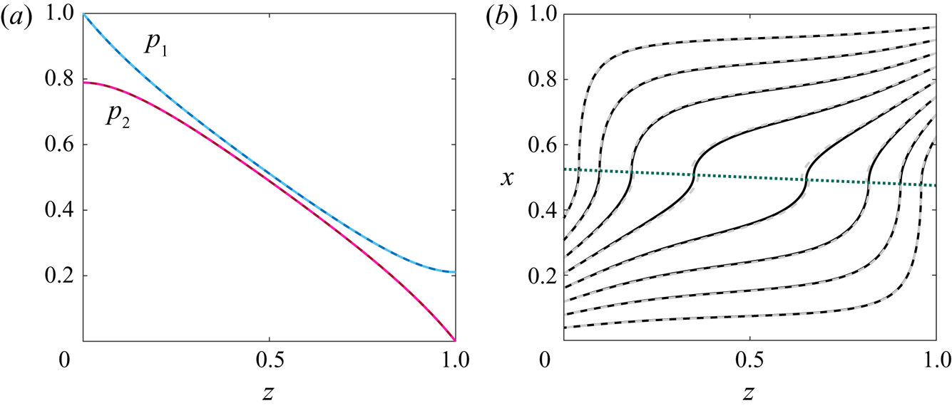
 $p_2$ using MATLAB's bvp4c solver (figure 2a). Using the solution for the pressures, we can calculate the velocity field in each subdomain using (2.20) and (2.23). A helpful way to visualise the qualitative behaviour of the flow through the domain is through its streamlines (figure 2b). We also present the flow field predicted by our asymptotic results (3.1) and (3.2) for
 $\beta \ll 1$,
 $a=O(1)$, derived in § 3.1.1, which shows excellent agreement with the numerical predictions.
Behaviour of the system governed by (2.21), (2.22) and (2.24), (2.25) for  $\beta = 0.05$,
 $a = 0.5$,
 $\kappa =1$ and
 $h=0$. The pressure profiles
 $p_1$,
 $p_2$ are shown in (a). The membrane position (dotted green line) as given in (2.12) and streamlines are shown in (b). We show both numerical solutions (solid) and asymptotic solutions (3.1) and (3.2) (dashed) and see excellent agreement.

We compare the flux (defined in (2.26)) predicted by the numerical results to that predicted by our asymptotic analysis for the two cases of  $a= O(1)$ (in § 3.1.1) and
 $a = O(\beta )$ (in § 3.1.2). The physically possible positions depend on the angle of the membrane:
 $a \in [\beta /2, 1-\beta /2]$. We note, however, that values of
 $a$ close to the boundaries of this interval are difficult to resolve numerically due to the presence of corners in the domain. We therefore solve for values of
 $a \in [ \beta /2+\delta _a, 1-\beta /2-\delta _a]$ for some small
 $\delta _a > 0$, and for all the results presented herein we take
 $\delta _a = 0.01$. To visualise the results we sample values of
 $\beta \ll 1$ and plot the resulting flux as a function of
 $a$.
There is excellent agreement between the numerical and analytic results for  $a= O(1)$ derived in § 3.1.1 (figure 3a). Importantly, we see that the flux is symmetric about
 $a=a^*:= 0.5$ where the midpoint of the membrane coincides with the midpoint of the domain. Moreover, for small
 $\beta$, the optimal flux occurs exactly at
 $a=a^*$, and so it is optimal to centre the membrane in the domain.
Flux  $Q$ given by (2.26) calculated from (2.21), (2.22) and (2.24), (2.25). Numerical solutions (solid line) compared with asymptotic results for
 $\beta \ll 1$ and
 $a= O(1)$ given by (3.1) and (3.2) (dashed line) and for
 $\beta ,\ a \ll 1$ given by (3.4) (dotted). Results shown for
 $a=O(1)$ in (a) and for
 $a\ll 1$ in (b) with
 $\kappa =1$,
 $h=0$ and
 $\beta = 0.04,\ 0.1,\ 0.16,\ 0.22$.

As we increase  $\beta$ (while still keeping
 $\beta$ small), the curve flattens around
 $a=a^*$ and the flux becomes fairly insensitive to variations in
 $a$ near
 $a^*$ (figure 3a). Eventually,
 $\partial ^2Q/\partial a^2(a^*,\beta ,1,0)>0$, indicating that the optimal location is no longer at
 $a=a^*$. However, the benefits of this optimal design over a centred design for
 $\beta \ll 1$ are marginal. In figure 3(b), we focus on the parameter regime where
 $a\ll 1$. As in the case when
 $a=O(1)$, we find that increasing the angle leads to higher fluxes. Moreover, our asymptotic results from § 3.1.2 show good agreement with the numerical results until
 $\beta$ gets too large.
The analysis of this section reveals two results: first, we can increase the flux through the device for the same applied pressure difference by tilting a horizontal membrane; second, for a small tilt, the flux is maximised when the membrane is located centrally, but as the membrane angle is increased the optimal location moves away from the centre. These observations motivate us to broaden our search to study the behaviour of the system for wider angled membranes in the following section.
3.2. Investigating the full angle domain
We now investigate the full angle domain, and examine the dependency of the optimal membrane position on the membrane angle. We continue to use  $h=0$ and
 $\kappa =1$ in this section, but consider general values of these in § 4. We present numerical solutions to (2.21) and (2.22) for
 $p_1$ in
 $\varOmega _1$ and (2.24) and (2.25) for
 $p_2$ in
 $\varOmega _2$ for all values of
 $a$ and
 $\beta$ in figure 4. Note that
 $\beta \in [0,1]$ and
 $a\in [\beta /2, 1-\beta /2]$. As mentioned in the previous section, numerical results are difficult to resolve for this system set-up when corners are present in the domain. We therefore explore the solution landscape for
 $\beta \in [0,1-\delta _\beta ]$, for some small
 $\delta _\beta >0$ and extrapolate our results to the full domain
 $\beta \in [0,1]$. In this paper, for all results shown, we take
 $\delta _\beta = 0.04$. Our domain for
 $a$ remains the same as before:
 $a \in [\beta /2+\delta _a, 1-\beta /2-\delta _a]$, and we extrapolate our conclusions to
 $a \in [\beta /2, 1-\beta /2]$.
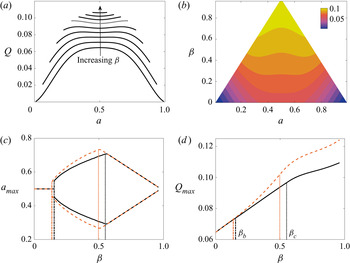
Solutions to (2.21), (2.22) and (2.24), (2.25). Numerical results (black, solid) and asymptotic solutions from (3.1) and (3.2) (orange, dashed) for  $\beta \in [0,1]$,
 $a \in [\beta /2, 1-\beta /2]$ with
 $\kappa =1$ and
 $h=0$. The dash-dotted lines indicate
 $\beta _b$ and the dotted lines indicate
 $\beta _c$. Panel (a) shows the flux
 $Q$ (2.26) for equally spaced
 $\beta \in [0, 0.87]$ inclusive, and (b) gives the contour plot of
 $Q$ in
 $(a,\beta )$-space. The optimal membrane position
 $a_{max}$ corresponding to the maximum flux achievable
 $Q_{max}$ (3.6) as a function of angle
 $\beta$ are shown in (c) and (d) respectively.

In § 3.1.3 we show that the flux increases with  $\beta$ for small
 $\beta$, and this trend remains true for larger values of
 $\beta$ (figure 4a). Moreover, in the same limit, we also show that the membrane position that maximises the flux moves away from the centre for increasing
 $\beta$. This trend continues in the full angle domain presented here; the optimal membrane position moves significantly off-centre as
 $\beta$ increases, bifurcating into two distinct optima symmetric about the centre of the domain for larger values of
 $\beta$ (figures 4(a) and 4(b)).
We define the position corresponding to the maximum achievable flux for a given angle by  $a_{max}(\beta )$. As
 $\beta$ increases, there is a bifurcation point
 $\beta = \beta _b$ at which the single, centred optimal design bifurcates into two off-centre optima, which drift further from the centre toward the corners of the domain as
 $\beta$ increases further (figure 4c). Thus, the bifurcation point
 $\beta =\beta _b$ marks a fundamental change in the optimal filter design. Due to the reversibility of Stokes flow, if one off-centre optimum exists then a second optimal configuration must exist in a set-up that is symmetric about
 $a=a^*$.
At a second critical value  $\beta = \beta _c > \beta _b$, the two optimal positions reach the corners of the physical domain, where they remain as
 $\beta$ increases further (figure 4c). We refer to
 $\beta _b$ and
 $\beta _c$ as the bifurcation and critical points, respectively. For
 $\beta > \beta _b$, we define the two optimal (off-centre) positions by
 $a^-$ and
 $a^+$ (with
 $a^- < a^+$ and
 $a^- + a^+ = 1$). When
 $\beta > \beta _c$, and the optimal membrane position consists of one membrane end residing at a corner of the domain, and we have
 $a^-=\beta /2$ and
 $a^+ = 1-\beta /2$.
As  $\beta _b$ is the lowest value of
 $\beta$ at which there is a local minimum in the flux at
 $a=a^*$, and recalling that the flux is symmetric about
 $a = a^*$,
 $\beta _b$ is implicitly defined by the condition
 \begin{equation} \frac{{\partial}^2 Q}{{\partial} a^2}(a^*,\beta_b,\kappa,h) = 0, \end{equation}
for a given  $\kappa$ and
 $h$. We determine
 $\beta _c$ by calculating the lowest value of
 $\beta$ for which the two off-centre optima are such that
 $a^-=\beta /2$ and
 $a^+ = 1-\beta /2$. Finally, to understand how the flux varies as these key values of
 $\beta$ are crossed, it is helpful to define the maximum flux achievable over
 $a$-space
 \begin{equation} Q_{max}(\beta, \kappa,h) = \mathop{\max}\limits_{a} Q(a,\beta,\kappa,h),\quad \mbox{for}\ a\in[\beta/2,1-\beta/2], \end{equation}
which occurs at  $a = a_{max}(\beta ,\kappa ,h)$.
For a membrane with permeance  $\kappa =1$ and thickness
 $h=0$, we see that
 $Q_{max}$ increases as
 $\beta$ increases (figure 4d). There does not appear to be any change in the qualitative behaviour of
 $Q_{max}$ around
 $\beta _b$, and this is consistent with the definition of
 $\beta _b$ in (3.5). That is, as the first and second derivatives of
 $Q$ with respect to
 $a$ both vanish at this critical point,
 $Q$ is fairly insensitive to
 $a$ near
 $a = a^*$,
 $\beta = \beta _b$. However, as
 $\beta$ passes through
 $\beta _c$, there is a change in the qualitative behaviour of
 $Q_{max}$. In particular, the slope of the curve decreases after this point, although we note that it does remain positive for these parameter values (
 $\kappa =1$,
 $h=0$). We will show later in § 4.1 that this is not always the case. Thus there are diminishing returns for
 $Q_{max}$ in terms of increasing
 $\beta$ beyond
 $\beta _c$.
In figures 4(c) and 4(d) we also present the small- $\beta$ results derived in § 3.1.1 alongside the numerical results from the full system. The asymptotic results agree very well with the numerical results for
 $a_{max}$ and
 $Q_{max}$ up to
 $\beta \approx 0.2$, and do predict the general trend thereafter, including the presence and effect of
 $\beta _b$ and
 $\beta _c$.
The results presented in this section show that angling the membrane away from horizontal can significantly increase the flux through a direct-flow device for the same applied pressure difference. Specifically, for a membrane with  $\kappa =1$ and
 $h=0$, angling the membrane away from horizontal can provide a 40 % increase in the maximum achievable flux (figure 4d). Moreover, we found that, while the optimal position for slightly tilted angles (with small
 $\beta$) is in the centre of the domain with
 $a=a^*$, the optimal position for increasing membrane angles bifurcates into two off-centre positions that move to the corner of the domain. Finally, the analysis of this section reveals the optimal set-up that maximises the flux through the membrane with
 $\kappa =1$ and
 $h=0$ to be a membrane centred and diagonal across the full domain (with
 $a=a^*$ and
 $\beta = 1$). We now turn to the wider aim of seeking the maximum achievable flux for a membrane of finite thickness and varying permeance by varying both the membrane position
 $a$ and the angle
 $\beta$.
4. Optimal position for a membrane of fixed properties
In this section we address the key motivating aim of determining the position and angle of a membrane of specified permeance and thickness that maximises the flux. In § 4.1, we retain our simplification of  $h=0$ and study membranes with varying permeance. In § 4.2 we relax this condition and examine the full problem with
 $h>0$.
4.1. Vanishingly thin membranes: $h= 0$

For a vanishingly thin membrane, we seek the optimal position and angle of a membrane of specified permeance  $\kappa$. We solve (2.21), (2.22) and (2.24), (2.25) numerically for
 $h=0$, and examine the flux (2.26) as we vary
 $\kappa$. Recall that the dimensionless resistance is simply the reciprocal of the permeance:
 $R = 1/\kappa$. Therefore, increasing the permeance decreases the resistance, and we observe the expected increase in the maximum flux achievable for a given
 $\beta$ (figure 5).


There is a quantitative change in the profiles of  $Q_{max}$ as a function of
 $\beta$ for increased
 $\kappa$ (figure 5). For small
 $\kappa$, the flux increases monotonically with
 $\beta$ and the optimal flux is achieved for
 $\beta = 1$ where the membrane is diagonal across the domain and centralised (
 $a=a^*$). For large
 $\kappa$, however, the highest flux is achieved when
 $\beta < 1$.
To examine at what position  $a$ this optimal flux is achieved, in this section we consider the critical angle
 $\beta_c$. We present the analysis of how the corresponding bifurcation angle
 $\beta_b$ varies with
 $\kappa$ in Appendix B. Recall that, for
 $\beta \geq \beta _c$, the maximum flux is achieved when either end of the membrane is positioned in a corner of the domain. We find that the optimal flux is achieved for angles slightly larger than
 $\beta _c$, and thus, for large
 $\kappa$, the optimal membrane position involves one end being in a corner of the domain. The associated optimal angle is predicted by the model equations (2.21), (2.22), (2.24), (2.25) and (2.26) through maximising
 $Q_{max}$ (3.6) as shown in figure 5. This result highlights the underlying physics in the problem. When optimising the flux, there is an inherent trade-off between maximising the length of the membrane and maximising the available space in one subdomain. Maximising the length of the membrane maximises the available surface area for ease of transport through the domain. Maximising the available space in either subdomain increases the transmembrane pressure drop. We find that for small
 $\kappa$, where the flow resistance is increased, it is more important to maximise the surface area of the membrane. Thus the optimal set-up is for the membrane to be diagonal across the full domain, thereby maximising the membrane length (figure 6a). For large
 $\kappa$, however, the membrane resistance is lower. In this case, it is more important to maximise the transmembrane pressure drop by shifting the membranes into the corners with increased available space in either subdomain (figure 6b). Thus, for large
 $\kappa$, the optimal angle is slightly larger than
 $\beta _c$ which is due to the trade-off between elongating the membrane and maximising the available space in either subdomain (figure 5).
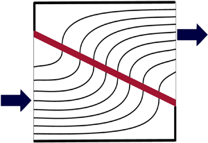
Schematics of the two dimensionless set-ups associated with optimal flux. The first, achieved for low permeances, is a centred membrane diagonal across full domain with  $\beta =1-h$ and
 $a=a^*$ as shown in (a). The second is an angled membrane in the corner with
 $\beta <1$ and
 $a=(\beta +h)/2$ as shown in (b). Note that the optimal configuration shown in (b) has an equivalent optimal configuration for the same optimal angle
 $\beta <1$ with
 $a = 1-(\beta +h)/2$. The full concertinaed device comprises repeated modules, and we illustrate this with faded schematics for the modules neighbouring the domain of consideration.

4.2. Membranes of finite thickness
We have so far restricted our attention to infinitely thin membranes, but in practice membranes have a finite albeit small thickness. We now relax this assumption to consider the effect of membrane thickness on the device behaviour. Hence, the new angle domain is  $\beta \in [0,1-h]$. We solve (2.21), (2.22) and (2.24), (2.25) numerically. As before, to avoid numerical complications arising from the presence of corners, we solve for
 $\beta \in [0, 1-h-\delta _\beta ]$ and
 $a\in [(\beta +h)/2-\delta _a, 1- (\beta +h)/2-\delta _a)]$, for some small
 $\delta _\beta , \delta _a >0$, and extend our conclusions to the full domain with
 $\delta _\beta ,\delta _a \to 0$.
In § 4.2.1, we first specify the permeance and focus on the effect of varying  $h$. In § 4.2.2, we then examine the combined effect of a finite thickness for varying permeance.
4.2.1. Investigating the effect of membrane thickness
We first examine the effect of a finite membrane thickness by varying  $h$ while holding
 $\kappa$ fixed. This corresponds to filters with different thicknesses but equal permeance, or equivalently equal net resistance. A helpful metric for comparison is
 $Q_{max}(\beta ,\kappa ,h)$, defined in (3.6), for varying
 $h$. For fixed permeance (and resistance), with
 $\kappa =1$, the maximum flux increases monotonically with
 $\beta$ and decreases as
 $h$ increases (figure 7a). Fixing the resistance isolates the effect of the geometry; as the membrane thickness increases, the membrane physically takes up more space and consequently inhibits the flow. We then consider the case where we vary
 $h$ and set
 $\kappa = 0.01/h$. Experimentally, this corresponds to comparing membranes made of the same material, so the permeability is the same, but the permeance or resistance changes accordingly with thickness. Increasing the thickness and decreasing the permeance (i.e. increasing the resistance) while holding the permeability constant decreases the maximum flux (figure 7b).
Maximum flux achievable  $Q_{max}$ given by (3.6) calculated from (2.21), (2.22), (2.24), (2.25) and (2.26). Results shown for
 $h=0$,
 $0.025$,
 $0.05$,
 $0.075$,
 $0.1$ with fixed permeance
 $\kappa =1$ in (a), and for
 $h=0.01$,
 $0.02$,
 $0.03$,
 $0.04$,
 $0.05$ with
 $\kappa =0.01/h$ (i.e. fixed permeability) in (b).

4.2.2. Quantifying the optimal design over experimental parameter space
Finally, we explore the full parameter space to understand what angle and position maximise the flux through the filter for a membrane of given thickness and permeance. We address this through consideration of the maximum achievable flux defined by
 \begin{equation}
\left.\begin{aligned} Q_{max}^*(\kappa,h) = \max_{a,\beta}
Q(a,\beta,\kappa,h) \quad & \mbox{for} \quad \beta \in[0, 1-h],
\nonumber\\ & \mbox{and} \ \ \,
a\in[(\beta+h)/2,1-(\beta+h)/2], \end{aligned}\right\}
\end{equation}
which we say occurs at  $\beta = \beta _{max}^*$ and
 $a=a_{max}^*$. Note that our earlier definition of
 $Q_{max}$ in (3.6) was introduced to find the optimal position associated with the maximum achievable flux for a membrane of specified angle, thickness and permeance. The definition of
 $Q_{max}^*$ in (4.1), however, seeks the optimal angle and position for a membrane of specified thickness and permeance.
The optimal angle and position are shown in figure 8. We immediately see that the profiles are discontinuous and this corresponds to the jump between the optimal positions depicted in figure 6. For smaller  $\kappa$, the optimal angle is
 $\beta _{max}^* = 1-h$ with the corresponding optimal position at
 $a_{max}^* = a^*$ (figure 8). (In fact, figure 8 shows that
 $\beta _{max}^* = 1-h-\delta _\beta$ which represents our numerically tested domain
 $\beta \in [0, 1-h-\delta _\beta ]$. We extrapolate our conclusions to the domain
 $\beta \in [0,1-h]$.) The set-up with
 $\beta_{\textit{max}}^* = 1-h$ is associated with the maximum achievable flux occurring for a centred membrane diagonal across the domain (as shown in figure 6a). As
 $\kappa$ increases, there is a critical value of
 $\kappa$ over which the optimal position jumps from the centre to the corner of the domain with the optimal angle occurring at
 $\beta _{max}^*< 1-h$, which is determined by our model, and the associated optimal position at
 $a_{max}^* = (\beta _{max}^*+h)/2$ (as shown in figure 6b). Sweeping across the full
 $\beta$-space (shown in figure 7) enables us to draw the conclusion that there exists a single optimal angle for all values of
 $\kappa$ except that at the transition point depicted by the discontinuity in figure 8(a).


Note that we have, without loss of generality, presented results for the branch of solutions corresponding to  $a_{max}^* = (\beta _{max}^*+h)/2$ only, but each off-centre optimal position is associated with a secondary optimal position symmetric about
 $a=a^*$, at
 $a_{max}^* = 1-(\beta _{max}^*+h)/2$ for the same
 $\beta _{max}^*$. Thus, for
 $\kappa$ above the critical value, the maximum flux is achieved for an angled membrane in the corner of the domain and the angle is determined by our model. Increasing
 $h$ results in the critical jump occurring for smaller
 $\kappa$ (figure 8).
The maximum achievable flux  $Q_{max}^*$ over a wide range of physical membrane properties is shown in figure 9. We observe that the global maximum
 $Q_{max}^*$ is achieved for
 $h \to 0$,
 $\kappa \to \infty$, with a horizontal membrane positioned in the corner (figures 8 and 9). Physically, this corresponds to maximally spaced infinitely thin membranes with zero resistance. In this case, the flux is maximised due to the pressure drop occurring almost entirely across the membrane. In practice, however, membrane design is limited in permeance and thickness. While figure 9 confirms that thinner, more permeable filters allow for greater flux, it provides a quantitative measure of how to design these filters for given membrane characteristics.
Maximum achievable flux  $Q_{max}^*$ in
 $(\kappa ,h)$-space defined by (4.1) calculated from (2.21), (2.22), (2.24), (2.25) and (2.26). The dashed line corresponds to the critical value of
 $\kappa$ at which there is a discontinuous jump from centred membranes to membranes in the corners. To the left of the dashed line, the maximum flux is achieved at centred membranes diagonal across the full domain; and to the right, the maximum flux is achieved at angled membranes in the corners of the domain.

Importantly, for any thickness and permeance, the maximum flux is achieved either for a centred membrane diagonal across the domain ( $(\kappa ,h)$-values to the left of the dashed line in figure 9) or for an angled membrane in the corner of the domain (
 $(\kappa ,h)$-values to the right of the dashed line in figure 9); i.e. the dashed line in figure 9 corresponds to the critical value of
 $\kappa$ over which there is a discontinuous jump in optimal design. Thus, a practitioner may use the model developed herein for a membrane of specified thickness and permeance to find the maximum achievable flux and the required angle and position that the membrane should take to achieve this flux. Specifically, if the membrane properties are to the left of the dashed line in figure 9, the optimal configuration is centred and diagonal across the domain, with angle
 $\beta ^*_{max} = 1-h$ and position
 $a^*_{max} = a^*$ (as depicted in figure 6a). If the membrane properties are to the right of the dashed line in figure 9, the optimal configuration is in either corner, and the angle
 $\beta ^*_{max}$ associated with maximum flux is provided by figure 8(a). The resulting optimal position is then
 $a^*_{max}=(\beta ^*_{max}+h)/2$ (or equivalently
 $a^*_{max}=1-(\beta ^*_{max}+h)/2$) as shown in figure 6(b).
5. Conclusions
In this paper, we studied the steady flow through a concertinaed direct-flow filtration membrane. The aim of the work was to find the geometry of the filtration membrane within a single repeating module that maximised the flux for a given pressure drop. The physical set-up facilitated a systematic asymptotic reduction of the mathematical system governing the flow. This resulted in a flow problem governed by two coupled lubrication-type equations. This system was characterised by four dimensionless parameter groupings, each representing different membrane properties; position  $a$, angle
 $\beta$, thickness
 $h$ and permeance
 $\kappa$.
We found that angling the membrane away from horizontal can greatly increase the flux through a direct-flow filtration device. For example, adjusting the device geometry for an infinitely thin membrane with fixed permeance  $\kappa =1$ can increase the flux through the device by up to 40 %. Moreover, for this specific membrane, we found that for slightly tilted membranes (with a small angle) the optimal position is in the centre of the domain. Increasing the membrane angle, however, results in the optimal position bifurcating to two off-centre optima which move to the corners of the domain as the angle increases. The global optimal set-up for this membrane was found to be a centred membrane diagonal across the full domain.
Extending our results to membranes of general physical characteristics, we found that there were two optimal membrane configurations. Below a critical permeance threshold, which we quantify, the membrane should be placed diagonally in a module in order to maximise membrane surface area. However, above this critical permeance threshold, the membrane should be placed in the corner of the module at an angle that depends on the system parameters, in order to maximise the transmembrane pressure drop. This discontinuity in the optimal system behaviour is summarised in figure 9, which provides a guide on which behaviour is optimal for given membrane properties and resulting maximum flux.
More generally, this work provides an example of a coupled problem in lubrication flow that exhibits non-trivial bifurcating optima symmetric about the centre of the domain. Although it is well known that free-boundary lubrication problems can yield interesting nonlinear results, our work shows that nonlinear outputs can also occur for coupled lubrication problems with fixed boundaries.
In practice, the filtration device we modelled is used to separate fluid mixtures. In this paper, we have studied the steady-state system relevant for early-time operation of newly manufactured filters, before blocking is significant, or for scenarios such as virus neutralisation where blocking never takes place. There are many applications of filtration, where later-time transient blocking can change the permeance and effective shape of the membrane separating the two fluid domains. A natural extension of the work presented here is to include transient blocking dynamics and study the optimal design of the filtration device to maximise the lifespan of these filters.
The findings in this paper can be used for any direct-flow filtration device with angled membranes. Practitioners may use the model presented herein to derive the optimal configuration for a membrane of specified thickness and permeance corresponding to the maximum possible flux through the device.
Acknowledgements
The authors would like to thank Smart Separations Ltd for presenting the initial problem, and Sotiria Tsochataridou from Smart Separations for many valuable discussions.
Funding
V.E.P. is supported by the EPSRC Impact Acceleration Account Award (grant no. EP/R511742/1). I.M.G. gratefully acknowledges support from the Royal Society through a University Research Fellowship.
Declaration of interests
The authors report no conflict of interest.
Appendix A. Asymptotic analysis
A.1. Membranes positioned close to the centre: $a=O(1)$

Applying the asymptotic expansion (3.1) to the governing equations (2.21) and (2.22) for  $p_1$ and (2.24) and (2.25) for
 $p_2$, and the membrane position
 $m(z)$ (2.12), gives the following leading-order problem:
 \begin{gather} a^3p_{10}'' = 3\kappa(\kern0.08em p_{10}-p_{20}),\quad p_{10}(0) = 1, \quad p_{10}'(1) = 0, \end{gather}
 \begin{gather}(a-1)^3p_{20}'' = 3\kappa(\kern0.08em p_{10}-p_{20}),\quad p_{20}(1) = 0, \quad p_{20}'(0) = 0. \end{gather}
We solve the coupled system of ODEs (A1) analytically, to yield
 \begin{align} p_{10} &= \frac{1}{N}\left[a^3 (1-a)^3 + a^6 \cosh(M) + (1-a)^6 \cosh(M(z-1))\right. \nonumber\\ &\quad + \left. a^3 (1-a)^3 \cosh(M z) - a^3 (1-a)^3 M(z-1)\sinh(M) \right], \end{align}
 \begin{align} p_{20} &= \frac{1}{N}\left[a^3 (1-a)^3 + a^6 \cosh(M) - a^3 (1-a)^3 \cosh(M(z-1))\right. \nonumber\\ &\quad -\left. a^6 \cosh(M z) - a^3 (1-a)^3 M (z-1)\sinh(M )\right], \end{align}
where
 \begin{equation} \left.\begin{gathered} \kappa_1 = \frac{3\kappa}{a^3}, \quad \kappa_2=\frac{3\kappa}{(1-a)^3},\quad M =\sqrt{\kappa_1+\kappa_2},\\ N = \left[(a^6 + (1-a)^6\right] \cosh(M) + a^3 (1-a)^3(2 + M \sinh(M)). \end{gathered}\right\} \end{equation}
Since this limit is a regular perturbation around  $\beta =0$, (A2) exactly solves the full problem described by (2.21), (2.22) and (2.24), (2.25) for a horizontal membrane.
At  $O(\beta$), we obtain the following system of ODEs and boundary conditions:
 \begin{align} \left[a^3p_{11}' + 3 a^2\left(\tfrac{1}{2}-z\right)p_{10}'\right]' = 3\kappa(\kern0.08em p_{11}-p_{21}),\quad p_{11}(0) = 0, \quad p_{11}'(1) = 0, \end{align}
 \begin{align}\left[(a-1)^3p_{21}'+ 3(a-1)^2 \left(\tfrac{1}{2}-z\right)p_{20}'\right]' = 3\kappa(\kern0.08em p_{11}-p_{21}), \quad p_{21}(1) = 0, \quad p_{21}'(0) = 0. \end{align}
Using variation of parameters, we derive the following analytic solutions to the system (A4):
 \begin{gather} p_{11} = \alpha_1(z) + \alpha_2(z) z + \kappa_1 \alpha_3(z) \cosh(Mz) + \kappa_1 \alpha_4(z) \cosh(M(z-1)), \end{gather}
 \begin{gather}p_{21} = \alpha_1(z) + \alpha_2(z) z - \kappa_2 \alpha_3(z) \cosh(Mz) - \kappa_2 \alpha_4(z) \cosh(M(z-1)), \end{gather}
where  $\alpha _i(z) = f_i(z) + c_i$ for
 $i = 1,2,3,4$, with
 \begin{gather} f_1(z) ={-}\frac{1}{M^2}\int_0^z s(\kappa_2 F_1(s) + \kappa_1 F_2(s))\,{\mbox{d}} s, \end{gather}
 \begin{gather}f_2(z) ={-}\frac{1}{M^2}\int_z^1 (\kappa_2 F_1(s) + \kappa_1 F_2(s))\,{\mbox{d}} s, \end{gather}
 \begin{gather}f_3(z) = \frac{\mbox{csch}(M)}{M^3}\int_z^1 \cosh(M(s-1))(F_2(s)-F_1(s))\,{\mbox{d}} s, \end{gather}
 \begin{gather}f_4(z) = \frac{\mbox{csch}(M)}{M^3}\int_0^z \cosh(M s)(F_2(s) - F_1(s))\,{\mbox{d}} s, \end{gather}
functions  $F_1$ and
 $F_2$ defined as
 \begin{gather} F_1(z) ={-} \frac{3}{a}\left[\left(\frac{1}{2}-z\right)p_{10}'\right]', \end{gather}
 \begin{gather}F_2(z) = \frac{3}{1-a}\left[\left(\frac{1}{2}-z\right)p_{20}'\right]', \end{gather}
and constants  $c_1, c_2, c_3, c_4$ that satisfy
 \begin{gather} 0 = c_1 + \kappa_1 (\,f_3(0) + c_3) + c_4 \kappa_1 \cosh(M), \end{gather}
 \begin{gather}0 = c_2 + \kappa_1 c_3 M \sinh(M), \end{gather}
 \begin{gather}0 = f_1(1) + c_1 + c_2 - \kappa_2 c_3 \cosh(M) - \kappa_2 (c_4 + f_4(1)), \end{gather}
 \begin{gather}0 = f_2(0) + c_2 + \kappa_2 c_4 M \sinh(M). \end{gather}
The system (A8) is derived from applying the boundary conditions in (A4) to (A5).
Since  $p_{10}$ and
 $p_{20}$ are given explicitly in (A2) and the system (A8) is linear, the solution (A5) represents an analytic solution to the
 $O(\beta$) problem. Moreover, we note that the integrals in (A6) can be evaluated explicitly, so our solution (A5) can be rewritten in closed form. However, the full expression is unwieldy, and does not provide any additional physical insight, so we do not present it herein. Hence, we have derived asymptotic solutions to the system (2.21), (2.22) and (2.24), (2.25) that are accurate up to
 $O(\beta ^2)$.
A.2. Membranes positioned close to the corner: $a=O(\beta )$

In this regime we can rewrite the membrane position (2.12) as
 \begin{equation} m(z) = \beta\left(A + \tfrac{1}{2}-z\right), \end{equation}
where  $A = a/\beta$ and simply consider the single limit
 $\beta \to 0$ with
 $A=O(1)$. Using (A9), the governing equations (2.21) and (2.22) for
 $p_1$ and (2.24) and (2.25)
 $p_2$ become
 \begin{gather} \beta^3 \left[ p_1'(A+\tfrac{1}{2}-z)^3\right]' = 3 \kappa (\kern0.08em p_1-p_2),\quad p_{1}(0) = 1, \quad p_{1}'(1) = 0, \end{gather}
 \begin{gather}\left[ p_2'(\beta(A+\tfrac{1}{2}-z)-1)^3\right]' = 3 \kappa (\kern0.08em p_1-p_2), \quad p_{2}(1) = 0, \quad p_{2}'(0) = 0. \end{gather}
In the limit of  $\beta \to 0$, the majority of the pressure drop across the system occurs near
 $z=0$. That is, there is a boundary layer of width
 $O(\beta ^{3/2})$, where
 $p_1$ drops from
 $1$ to being of
 $O(\beta ^{3/2})$, and
 $p_1= O(\beta ^{3/2})$ away from this boundary layer. Moreover,
 $p_2 =O(\beta ^{3/2})$ everywhere in
 $\varOmega _2$. To derive the solution in this boundary layer we introduce the boundary layer variable
 \begin{equation} z = \beta ^{3/2} Z, \end{equation}
which scales the system of ODEs (A10) to obtain the leading-order boundary layer problem
 \begin{gather} \left(A+\frac{1}{2}\right)^3\frac{{\mbox{d}}^2 p_1}{{\mbox{d}} Z^2} = 3 \kappa (\kern0.08em p_1-p_2),\quad p_{1}(0) = 1,\quad p_{1}'(\infty) = 0, \end{gather}
 \begin{gather}- \frac{{\mbox{d}}^2 p_2}{{\mbox{d}} Z^2} = 0,\quad p_{2}(\infty) = 0,\quad p_{2}'(0) = 0, \end{gather}
where the conditions as  $Z \to \infty$ arise from matching into the outer regions where
 $p_1, p_2 = O(\beta ^{3/2})$. The system (A12) is solved by
 \begin{gather} p_1 = \exp\left[ - \left(\frac{3\kappa}{\left(A+\frac{1}{2}\right)^3}\right)^{1/2} Z\right] = \exp\left[ - \left(\frac{3\kappa}{\left(a+\frac{1}{2}\beta\right)^3}\right)^{1/2} z\right], \end{gather}
 \begin{gather}p_2 = 0, \end{gather}
and we note that the  $O(\beta ^{3/2})$ terms can be calculated if required.
Appendix B. Bifurcation point
In this appendix, we consider infinitely thin membranes with  $h=0$, and examine the maximum flux achievable for membranes of varying permeance
 $\kappa$. Specifically, we are interested in the values of
 $\beta$ and
 $\kappa$ for which there exists a bifurcation point
 $\beta _b$. This is calculated by formulating the flux function
 $Q(a^*, \beta , \kappa ,0)$ from (2.26) and deriving the domain corresponding to
 ${\partial } Q^2/{\partial } a^2 (a^*,\beta ,\kappa ,0) > 0$, for which a minimum exists at
 $a=a^*$ and consequently where two distinct optima co-exist. Thus we construct a phase diagram in
 $(\beta ,\kappa )$-space (figure 10). We denote the domain in which one finds a single optimal position by
 $\varLambda _1$ and that in which there are two optimal positions by
 $\varLambda _2$.
Phase diagram showing where one optimum membrane configuration exists in  $\varLambda _1$ and where two optimum configurations exist in
 $\varLambda _2$ in (
 $\beta ,\kappa$)-space;
 $\varLambda _2$ indicates the values
 $(\beta ,\kappa )$ for which
 ${\partial }^2 Q/{\partial } a^2 (a,\beta ,\kappa ,0)>0$, where
 $Q$ is calculated from (2.26) using the solutions from (2.21), (2.22) and (2.24), (2.25). The numerical results show the two shaded regions, and the analytical results are used to plot the black-dashed curve between them.

For permeances  $\kappa \gtrsim 1.2$, the presence of the
 $\varLambda _2$ region indicates that there are two distinct optimal positions for the membrane angles
 $\beta \lesssim 0.96$ (figure 10). For
 $0.96\lesssim \beta \leq 1$, there is a single optimal position. This is because larger values of
 $\beta$ provide tighter constraints on the membrane position within the domain, and so only one position is possible, namely the centred membrane,
 $a=a^*$. For permeances
 $\kappa \lesssim 1.2$ there is a distinctive curve separating the two regions, across which a single optimal position bifurcates into two off-centre optimal positions. Thus we conclude that
 $\beta _b$ exists only for small
 $\kappa \lesssim 1.2$.
We also show the equivalent analytic results from § 3.1.1 in figure 10. Using the analytic expressions for the pressure in (3.1), we are able to calculate an explicit form for the curve  ${\partial } Q^2/{\partial } a^2(a^*,\beta , \kappa ,0)=0$, which we show in figure 10 as a dashed line. This shows excellent agreement with the numerical results even up to intermediate values of
 $\beta$, despite the asymptotic results only being valid for small
 $\beta$. The asymptotic results do diverge significantly after
 $\beta \gtrsim 0.96$, since the asymptotic results do not account for the constraints in membrane position that occur at larger values of
 $\beta$.