Introduction
Residual strain is the strain that remains after the original cause of the external stress has been removed [Reference Li, An, Liu and Wang1]. Residual strain occurs for a variety of reasons, such as when materials were subjected to the tension load, random vibration, or high impact [Reference Zhang, Huang, Bian and Wan2]. Residual strain is a significant factor for assessing the deformation and failure of materials [Reference Withers3]. Simultaneously, the residual strain in metal could make significant effect to the change of measured lattice parameters, which potentially leads to inaccurate structural integrity evaluation and determination [Reference Li, An, Liu and Wang1].
The nonlinear ultrasonic technique is a novel method emerging in recent years [Reference Zheng, Maev and Solodov4, Reference Breazeale and Thompson5, Reference Mondal, Mukhopadhyay and Sarkar6, Reference Jhang7, Reference Baby, Kowmudi, Omprakash, Satyanarayana, Balasubramaniam and Kumar8], and now it has been recognized as a powerful method for characterizing the microstructural features in solids. With respect to its application in metal, a review of this technique was provided by Matlack [Reference Matlack, Kim, Jacobs and Qu9]. Recently, Apple et al. [Reference Apple, Cantrell, Amaro, Mayer, Yost, Agnew and Howe10] studied the nonlinear effect in single crystal copper during the fatigue process and found that the variation of nonlinear parameter was related to the presence of secondary dislocations in the samples. Xiang et al. [Reference Xiang, Deng, Xuan and Liu11] studied the thermal degradation in ferritic Cr–Ni alloy steel and revealed that the acoustic nonlinearity increases due to the second phase precipitates in the early stage; Marino et al. [Reference Marino, Kim, Ruiz, Joo, Qu and Jacobs12] investigated the thermal aging in 9% Cr steel and found that the nonlinearity of material is sensitive to the variation of precipitate density. On the basis of the past investigations, the causes of the nonlinear effect in metal can be summed up as the following: (i) fatigue-induced microvoids and microcracks; (ii) the lattice distortion resulted from the tensile damage; (iii) the dislocation density rises and the phenomenon of dislocation pile-up occurs; (iv) the precipitated phases coarsening and its interaction with dislocations.
Although some of the works have been done in the past; however, with regard to the physical damage in metal, previous nonlinear ultrasonic studies were confined to the fatigue damage that happen at the plastic stage. With respect to the microresidual strain in metal that happen within the range of elasticity, comprehensively experimental investigations are still rare. Considering the practical application of the metal components was usually subjected to a load below its elastic limit; therefore, it is even more desirable to characterize the variation of material property at this region.
X-ray diffraction (XRD) is a general way to characterize the residual strain in materials, but this method was time consuming, since it requires the process of sample preparation. The advantages of such an ultrasonic technique are intuitively clear, which can provide a quick start, a faster data return, and relatively simple measurement setup. Under this circumstance, it is necessary to establish the quantitative relationship between the nonlinear response and microresidual strain. That is what we intended to do and have done in this research for a typical industrial material undergone elastic loading. The reason for choosing the mild steels is due to its wide applications in the construction and equipment manufacturing industry.
Ultrasonic nonlinearity
The nonlinear elastic properties of solids containing microdefects (scaled from dislocations to volume inclusions) or structural changes can be manifested in specific types of ultrasonic nonlinearity. Through the measurements of the higher order elastic constants of material, the acoustic–elastic properties of a solid can be determined. For instance, second harmonic generation measurements have shown to be very applicable in detecting microstructural changes in metals, which are most commonly used with the longitudinal waves.
In a solid element, the stress σ–strain ε relation relationship in a nonlinear medium [Reference Cantrell and Yost13, Reference Zhu, Xiang, Liu, Deng, Ma and Xuan14, Reference Xiang, Deng, Xuan and Liu15, Reference Pešička, Kužel, Dronhofer and Eggeler16, Reference Sun, Xiang, Deng, Tang, Zhu and Xuan17] can be written as the following:
 $$\sigma = E\varepsilon \left( {1 + \beta \varepsilon + \cdots } \right)\quad ,$$
where E is the elasticity modulus and β is the second-order nonlinear parameter.
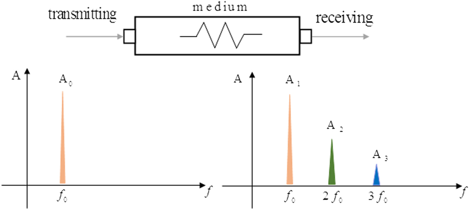
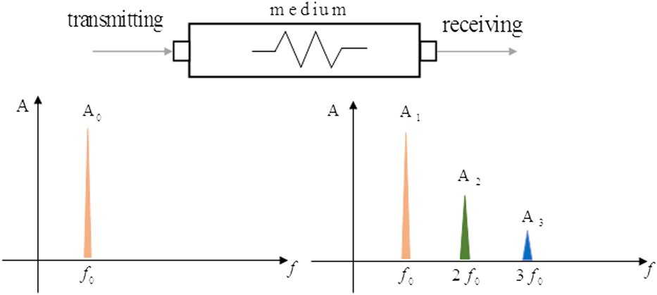
When a sinusoidal ultrasonic wave of a single frequency with sufficient strength is introduced into an anharmonicity solid, the fundamental wave will be distorted by the nonlinear elastic response as it propagates, so that the second and higher harmonic waves are generated in transmitted wave (as shown in Fig. 1). The f 0 represents the initial wave frequency, and 2f 0 and 3f 0 are the second and third-order terms of the harmonic frequency component, respectively.
Distortion in the waveform during propagation and harmonic generation.
In the meantime, the motion equation of longitudinal wave in a material can be described as the following [Reference Kim, Park and Jhang18]:
 $$\rho {{{\partial ^2}u} \over {\partial {t^2}}} = {{\partial \sigma } \over {\partial x}}\quad ,$$
where ρ is the medium mass density, u is the medium displacement, t is the time, σ is the stress, and x is the wave propagation distance. Meanwhile, the relationship between ε and u can be given as:
 $$\varepsilon \left( {x,t} \right) = {{\partial u\left( {x,t} \right)} \over {\partial x}}\quad .$$
Combined Eqs. (1), (2), and (3), the nonlinear wave equation can be obtained as
 $$\rho {{{\partial ^2}u} \over {\partial {t^2}}} = E\left( {{{{\partial ^2}u} \over {\partial {x^2}}} + 2\beta {{\partial u} \over {\partial x}}{{{\partial ^2}u} \over {\partial {x^2}}}} \right)\quad .$$
Consider a sinusoidal wave u = A sin ωt, where A 1 is the fundamental wave amplitude, A 2 is the second harmonic, ω is the angular frequency, and k is the wave number. Then the nonlinear parameter β can be determined in terms of the A 1, A 2, k, and x [Reference Matlack, Kim, Jacobs and Qu9],
 $$\beta = {8 \over {{k^2}x}}{{{A_2}} \over {A_1^2}}\quad .$$
Since the harmonic wave amplitude was related to the medium properties, therefore, one can assess the degradation of medium by measuring the harmonic wave amplitude generated in the transmitted wave. Besides, to simplify the algorithm, it can also use the  $\beta ' = {{{A_2}} / {A_1^2}}$ to replace β.
Result and discussion
Ultrasonic measurement
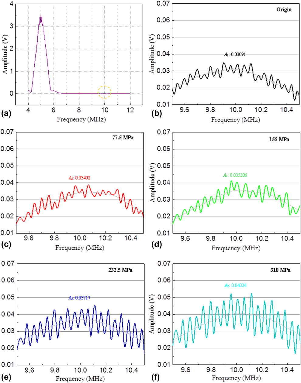
Figure 2(a) shows the frequency-amplitude function of the original mild steel specimen. The spectrum curve contains both the output frequency signal of 5 MHz fundamental wave (A 1) and 10 MHz second-order harmonic wave (A 2). In general, the A 2 is an important parameter of studying the material degradation or microstructure and property variation. Nevertheless, the change of the second-order harmonic wave was typically small, and it was hard to identify the change of A 2 when both A 1 and A 2 were in one frequency spectrum. Under this circumstance, to make the accurate observation of the A 2 variation, we focus on the frequency domain that range from 9.5 to 10.5 MHz, which was marked with a loop.
The spectrum curve and the variation of A 2 in mild steel specimen. (a) The spectrum curve of the original mild steel specimen. (b) The A 2 of the origin specimen. (c) The A 2 of the specimen stretched to 77.5 MPa. (d) The A 2 of the specimen stretched to 155 MPa. (e) The A 2 of the specimen stretched to 232.5 MPa. (f) The A 2 of the specimen stretched to 310 MPa.
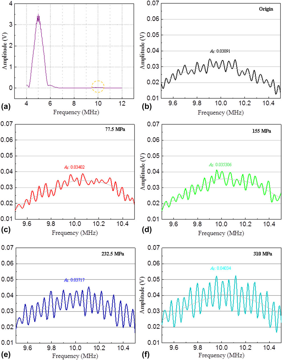
Figures 2(b)–2(f) show the variation of A 2 in mild steel specimen with different tensile stresses. It can be observed that there was a rising tendency of second harmonic amplitude with the increase of applied stress, which indicates that the nonlinearity effect has accumulated in the tensile specimens. The change of A 2 was relatively small when applied stress was below 155 MPa, but increases notably when stress was above 232.5 MPa. Although the growth trend of second harmonic wave can be clearly recognized, a tooth-like oscillation makes it hard to determine the accurate value of A 2. Under this circumstance, the harmonic signal of A 2 was smoothed in MATLAB-2016 by using the algorithm of linear weighting.
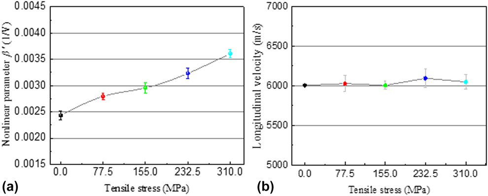
A similar pattern was also found in the change of the nonlinear parameter. To make sure that the reproducibility and reliability of this test, each measurement was repeated four times. Through recording the fundamental (A 1) and the corresponding second harmonic (A 2) amplitude in each file, the nonlinear parameter β′ can be calculated. Figure 3(a) shows the variation of nonlinear parameter with different tensile stresses in the mild specimen. From this experimental result, we can see that the nonlinear parameter gradually increases with increasing applied stress. To compare with the original specimen, the nonlinear parameter rose beyond 40% when it stretched to 310 MPa, which indicates that the nonlinearity effect was accumulating with the increase of applied stress.
The ultrasonic measurement of the mild steel specimens with different tensile stresses. (a) Variation of the nonlinear parameter in mild steel specimens with different tensile stresses. (b) The longitudinal velocity in mild steel specimens with different tensile stresses.
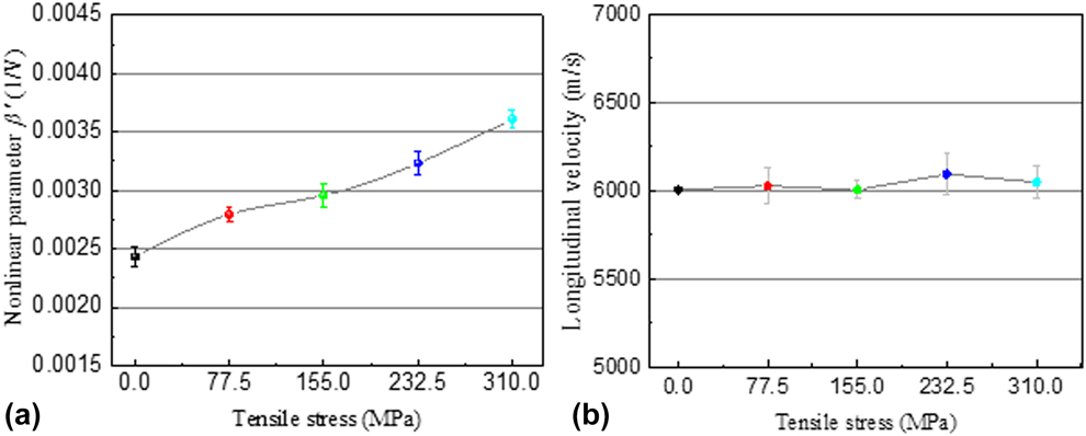
The higher sensitivity of nonlinear ultrasonic measurements can be demonstrated when Fig. 3(a) is compared against the results obtained from the traditional longitudinal wave velocity measurements. From Fig. 3(b), it can be seen that the longitudinal velocity of mild steel remains almost unchanged from original condition to stretch to 155 MPa and then shows a small rise of approximately 0.0189% when the specimen was stretched to 232.5 MPa, but returns later at the elastic limit. In fact, the longitudinal velocity in this research did not exhibit a linear increase within the elastic region, which indicates that the traditional ultrasonic measurements are not sensitive enough to the microresidual strain. Virtually, the longitudinal velocity decreases notably only when the metal undergone a dramatic change. From these results, the higher sensitivity and superiority of the nonlinear ultrasonic technique can be fully realized.
Based on the principles of the nonlinear elasticity theory, the material failure or degradation was usually preceded by some kind of nonlinearity behavior, so that the waveform of incident signal is distorted by the nonlinear elastic response [Reference Xiang, Deng, Xuan and Liu15]. Recent studies [Reference Matlack, Kim, Jacobs and Qu9, Reference Apple, Cantrell, Amaro, Mayer, Yost, Agnew and Howe10, Reference Herrmann, Kim, Jacobs, Qu, Littles and Savage19, Reference Valluri, Balasubramaniam and Prakash20] show that there are three determining factors that can lead to the increase of the nonlinear parameter, which include the microvoid formation, the lattice distortion, and the increase of dislocation density. In order to figure out the causes of nonlinear parameter increase within the elastic stage, the microstructure of mild steel specimen was investigated after the tensile testing.
Microscopic structures observation
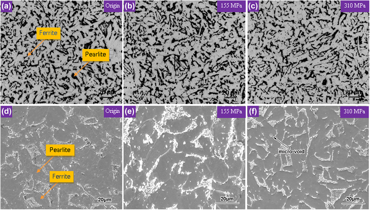
Microscopic structures of mild steel were observed before and after the tensile test. The OM micrographs of mild steel specimens are shown in Figs. 4(a)–4(c), and the SEM micrographs of this steel are shown in Figs. 4(d)–4(f). In OM observation, it can be seen that microstructures of this steel are pearlite and ferrite. And in SEM observation, the pearlite shows irregular lamellar as well as dendritic shape that distributed homogenously around the ferrite matrix. In comparison with Fig. 4(d), apart from one, microvoids (about 1 μm) had appeared in Fig. 4(f) and no appreciable microstructural change can be observed. Virtually, a significant increase in void number density and dimension can only happen during the severe plastic deformation; hence, the void contribution to the nonlinearity change in the elastic range can be negligible.
Microstructures of the mild steel specimens under different tensile stresses. (a) OM image of the origin specimen. (b) OM image of the specimen stretched to 77.5 MPa. (c) OM image of the specimen stretched to 155 MPa. (d) SEM image of the origin specimen. (e) SEM image of the specimen stretched to 155 MPa. (f) SEM image of the specimen stretched to 310 MPa.
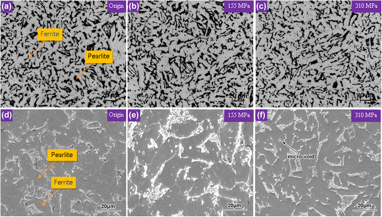
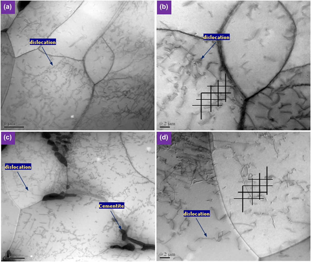
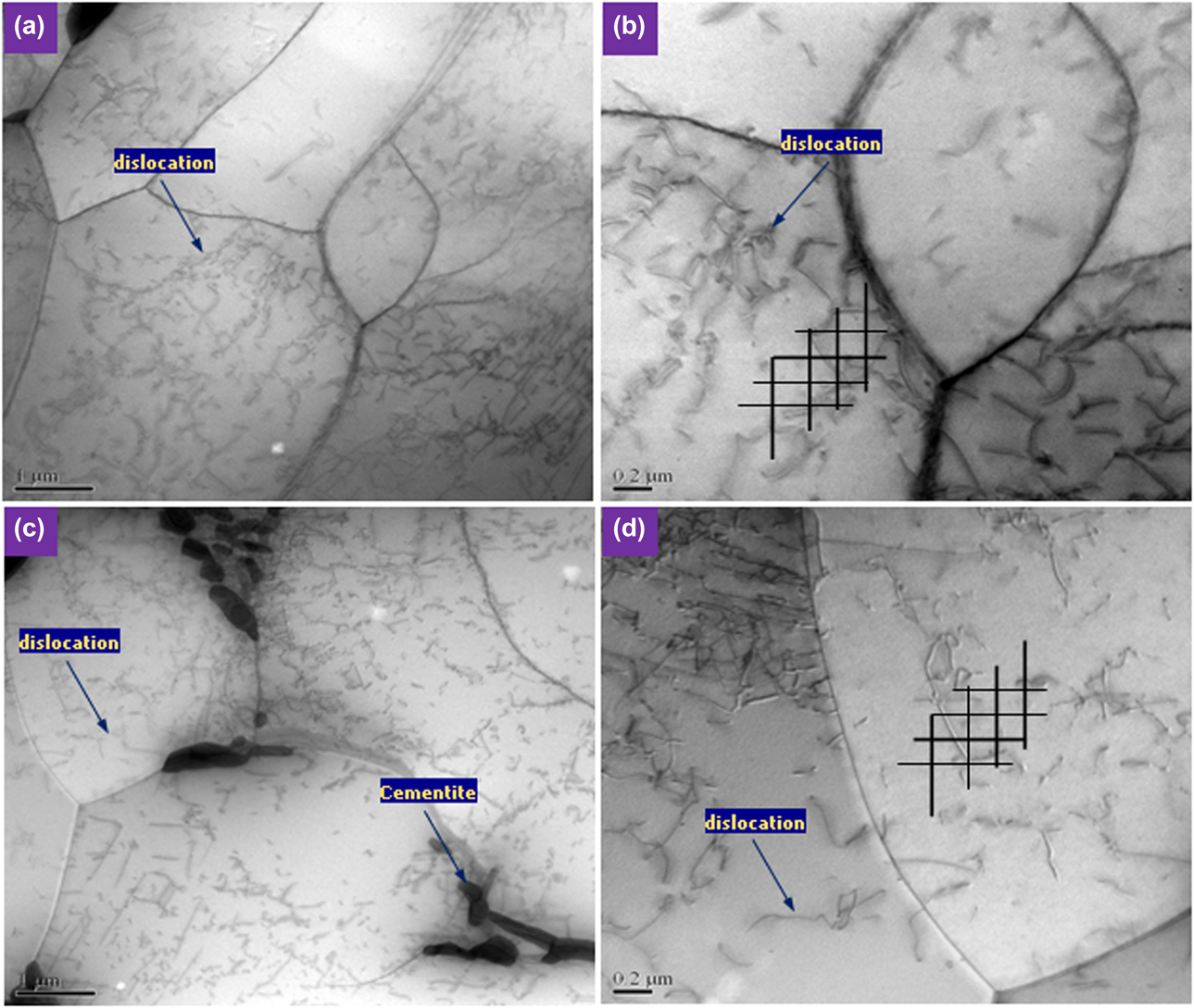
Figure 5 shows the TEM images of the original and the tensile mild steel specimens. The streak and rod-like cementite distributed randomly along ferrite grain boundary [see Fig. 5(c)] and a certain amount of dislocation have been observed in the original specimen with a labyrinth structure [see Fig. 5(a)]. However, with respect to the dimension and number density of dislocation lines, no distinct changes have been found in the tensile specimen. Here, the dislocation density was calculated by using the method proposed from Pešicka et al. [Reference Pešička, Kužel, Dronhofer and Eggeler16], which drew the random lines for counting the number of dislocation intersections on the micrographs, then the density can be figured out from the following expression:
 $$\Lambda = {1 \over t}\left[ {{{\sum {n_{\rm{v}}}} \over {\sum {L_{\rm{v}}}}} + {{\sum {n_{\rm{h}}}} \over {\sum {L_{\rm{h}}}}}} \right]\quad ,$$
where t is the thickness of the slice (200 nm), n v and n h are the number of dislocations crossing a vertical line and a horizontal line, respectively. L v and L h are the values of the vertical line and the horizontal line, respectively. The results indicate that the dislocation density of the original specimen and 310 MPa tensile specimen were 4.864 × 10¹³ m−2 and 4.891 × 10¹³ m−2, which corresponds to Figs. 5(b) and 5(d). From this result, it can be recognized that the dislocation density did not occur a significant change within the elastic stage; therefore, it can be concluded that the nonlinear parameter increase in this region may not come from the contribution of dislocation variation.
TEM images of this mild steel before and after the tensile test. (a) Original specimen at low magnification. (b) Original specimen at high magnification. (c) Tensile specimen at low magnification. (d) Tensile specimen at high magnification.
The microresidual strain characterization in specimen
The microresidual strain measurement
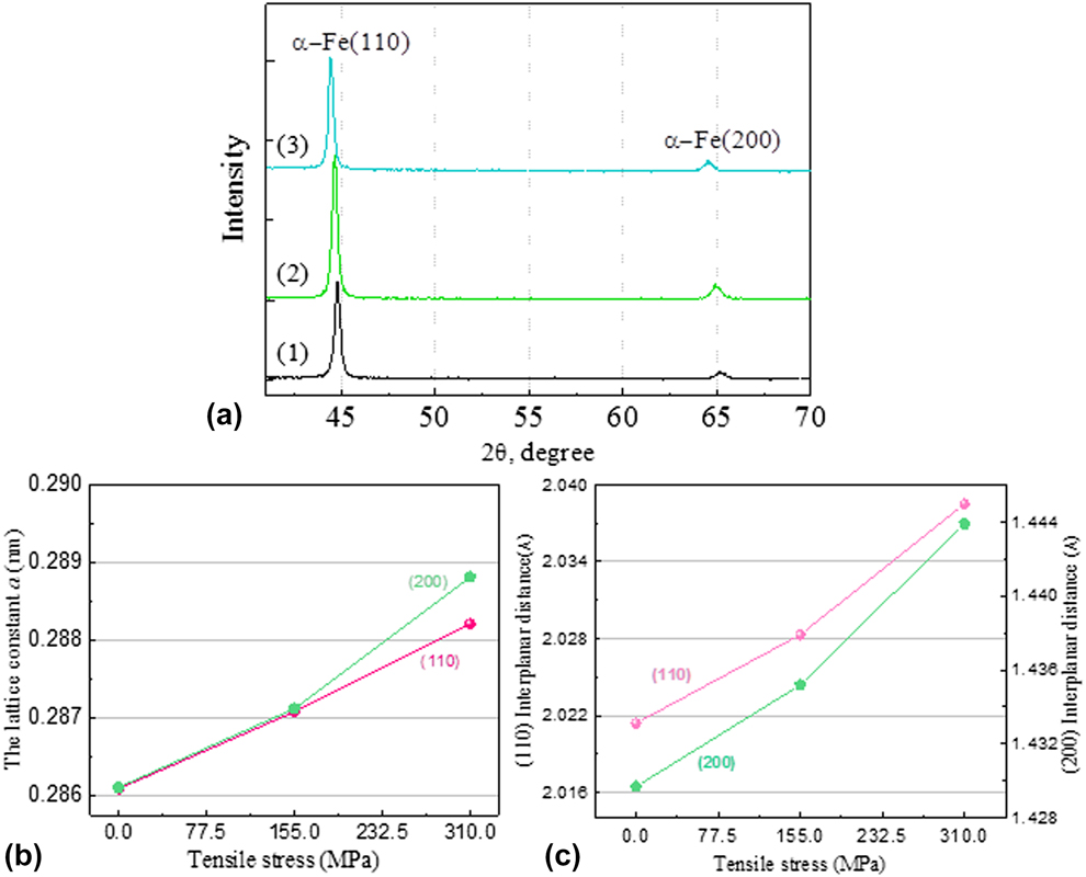
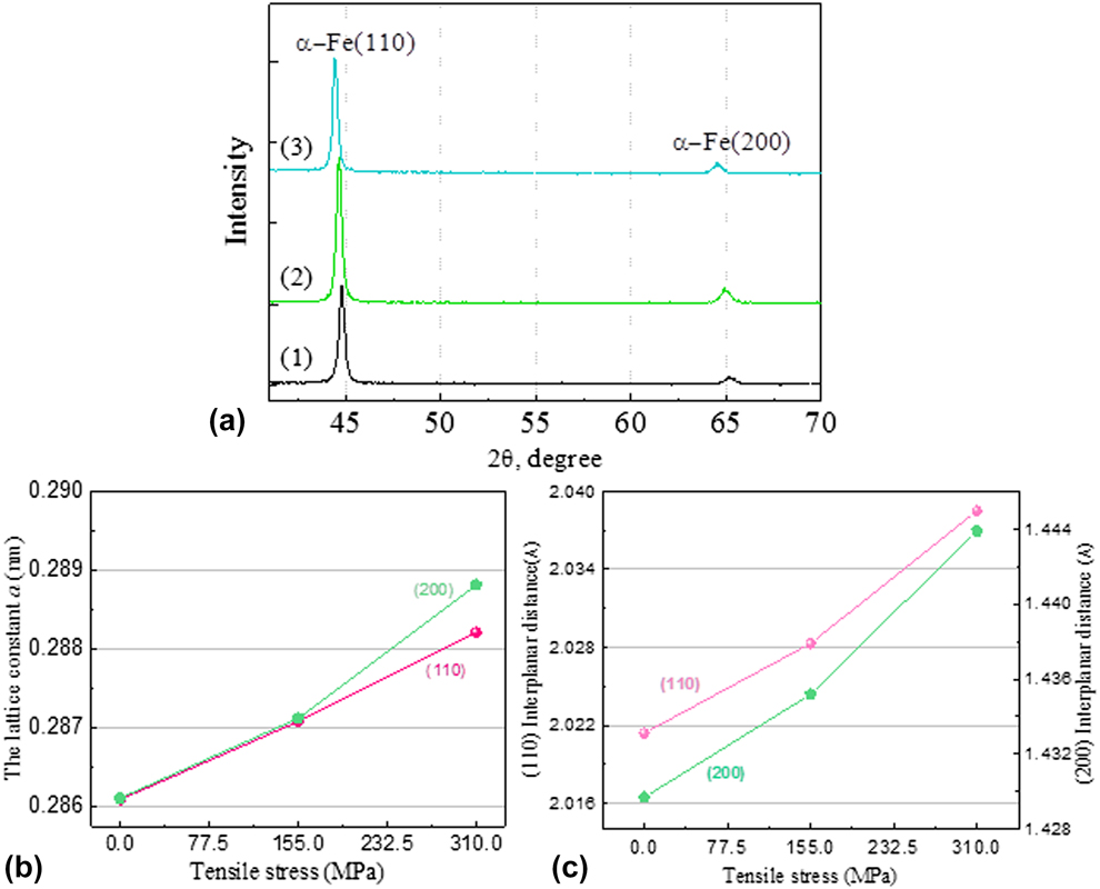
Precise lattice parameter measurement is of great help to understand the cause of nonlinear parameter variation. As shown in Fig. 6(a), in the original specimen, the lattice plane of (110) and (200) appears the α-Fe diffraction peak, where at 2θ = 44.770° and 2θ = 65.132°. With the applied stress increased, both of two diffraction peaks exhibit a lateral shift (to the left), and this deviation gets the maximum as tensile stress increased to the elastic limit (310 MPa), which equals to 0.357° and 0.654°, respectively. It is important to realize that shifting of diffraction peaks arises mainly due to the lattice distorting as well as grain deformation [Reference Kanjarla, Lebensohn, Balogh and Tomé21, Reference Huang, Barabash, Clausen and Liaw22]; here, the variation of the lattice constant a and interplanar spacing d hkl for both lattice plane is shown in Figs. 6(b) and 6(c).
XRD measurement results of mild steel specimens under different tensile stresses. (a) The X-ray diffraction patterns of mild steel specimens. (1) Origin. (2) 155 MPa. (3) 310 MPa. (b) The variation of the lattice constant of the mild steel specimens. (c) The variation of the interplanar spacing of the mild steel specimens.
As we know, the variation of the lattice constant and interplanar spacing was usually associated with the internal strain in material. The relationship between the changes of Bragg angle with interplanar spacing can be given as
 $${\rm{d}}\theta = \theta - {\theta _0} = - \tan \;{\theta _0}\left( {{{{\rm{d}}D} / {{D_0}}}} \right) = - \tan \;{\theta _0}\left[ {{{\left( {D - {D_0}} \right)} / {{D_0}}}} \right]\quad ,$$
where θ and θ0 are the Bragg angle before and after the tensile testing. D and D 0 are the interplanar spacing under strain condition and no strain condition. Meanwhile, the microresidual strain εhkl of mild steel can be calculated utilizing Bragg’s law,
 $${\varepsilon _{hkl}} = {{\left( {{d_{hkl}} - d_{hkl}^0} \right)} \over {d_{hkl}^0}}\quad ,$$
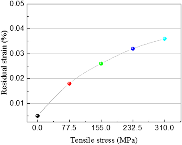
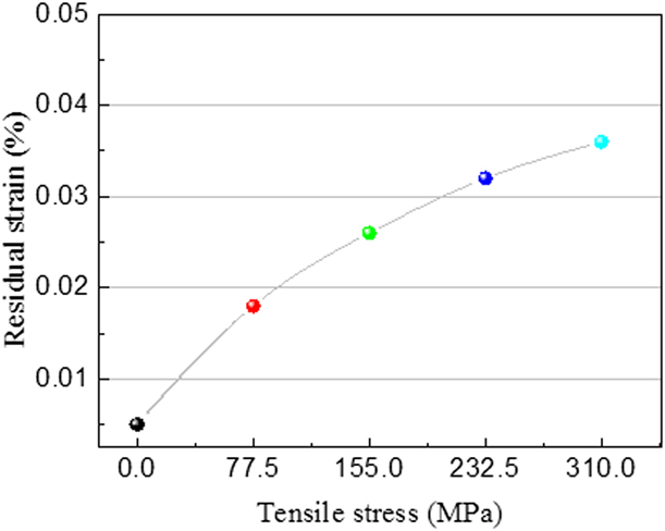
where  $d_{hkl}^0$ is the stress-free lattice spacing. Figure 7 shows the effect of applied stress on residual strain in mild steel specimen, and it can be observed that the microresidual strain accumulated as early as at the low stress region. Theoretically, in an ideal scenario, the strain recovery is one of the most basic characteristics in metallic material within the elastic deformation, since the order degree of crystalline (i.e., entropy value) has been basically unchanged. When the applied load is removed, the reduction of the internal energy could drive the elastic recovery; however, in the real situation, any material is a nonideal linear solid, because of the effects of retarded elasticity, the absorbed energy of the material in the process of loading is always greater than it is discharged during the release loading (i.e., internal friction), which causes the microstrain residues in the solid. And if the situation is serious enough in engineering application, we must take this case into consideration.
The variation of residual strain in mild steel specimen with different tensile stresses.
The nonlinearity calculation in mild steel with microresidual strain
An initially sinusoidal acoustic wave will generate harmonics of the fundamental waveform as it propagates through a solid as the result of the nonlinearity of the propagation medium [Reference Xiang, Deng, Xuan and Liu11, Reference Marino, Kim, Ruiz, Joo, Qu and Jacobs12]. Cantrell and Yost [Reference Cantrell and Yost13] reported that disruptions in the crystal lattice can lead to considerable changes in the amplitude of the nonlinear parameters. For isotropic symmetry polycrystalline alloys, the parameter can be written using the Voigt contraction of indices,
 $${\beta _0} = - \left( {{{3{{\bar{C}}_{11}} + {{\bar{C}}_{111}}} \over {{{\bar{C}}_{11}}}}} \right),\;\beta = - \left( {{{3{C_{11}} + {C_{111}}} \over {{T_{11}} + {C_{11}}}}} \right)\quad ,$$
where β0 is the nonlinearity parameter referred to the zero stress state, β is the nonlinearity parameter of material that after the stress effects. The quantities T 11, C 11, and C 111 for isotropic symmetry can be expressed as the following:
 $$\eqalign{ & {T_{11}} = {{\bar{C}}_{11}}{n_{11}} + {{\bar{C}}_{12}}\left( {{n_{22}} + {n_{33}}} \right) + \cdots \cr & {C_{11}} = {{\bar{C}}_{11}} + \left[ { - {{\bar{C}}_{11}}\left( {{n_{11}} + {n_{22}} + {n_{33}}} \right) + 4{{\bar{C}}_{11}}{n_{11}} + {{\bar{C}}_{111}}{n_{11}} + {{\bar{C}}_{112}}\left( {{n_{22}} + {n_{33}}} \right)} \right] + \cdots \cr & {C_{111}} = {{\bar{C}}_{111}} + \left[ { - {{\bar{C}}_{111}}\left( {{n_{11}} + {n_{22}} + {n_{33}}} \right) + 6{{\bar{C}}_{111}}{n_{11}} + {{\bar{C}}_{1111}}{n_{11}} + {{\bar{C}}_{1112}}\left( {{n_{22}} + {n_{33}}} \right)} \right] + \cdots \quad , \cr}$$
where n ii are the strains corresponding to the deformation of material (n ii = εii),  ${\bar{C}_{ijkl}}$ and
 ${\bar{C}_{ijklmn}}$ are the second and third order Brugger elastic constants referred to the zero stress state. Substituting Eq. (9) into Eq. (10), the calculation of parameter variation Δβc that results from the residual strain can be obtained as
 $$\Delta {\beta _{\rm{c}}} = \beta - {\beta _0} = \left( {3 - {{{{\bar{C}}_{111}}} \over {{{\bar{C}}_{11}}}} - {{{{\bar{C}}_{1111}}} \over {{{\bar{C}}_{11}}}} + {{\bar{C}_{111}^2} \over {\bar{C}_{11}^2}}} \right){\varepsilon _{11}} + \left( {3{{{{\bar{C}}_{12}}} \over {{{\bar{C}}_{11}}}} - {{{{\bar{C}}_{1112}}} \over {{{\bar{C}}_{11}}}} + {{{{\bar{C}}_{12}}{{\bar{C}}_{111}}} \over {\bar{C}_{11}^2}} + {{{{\bar{C}}_{112}}{{\bar{C}}_{111}}} \over {\bar{C}_{11}^2}}} \right)\left( {{\varepsilon _{22}} + {\varepsilon _{33}}} \right)\quad .$$
Meanwhile, in the case of the uniaxial tension test, we have
 $${\varepsilon _{22}} = {\varepsilon _{33}} = - \mu {\varepsilon _{11}}\quad ,$$
where μ is the poisson’s ratio of mild steel. Using the Hiki–Granato relationship here (i.e.,  ${\bar{C}_{11}} = 2{\bar{C}_{12}}$,
 ${\bar{C}_{111}} = 2{\bar{C}_{112}}$,
 ${\bar{C}_{1111}} = 2{\bar{C}_{1112}}$,
 ${{{{\bar{C}}_{111}}} / {{{\bar{C}}_{11}}}} \approx {{{{\bar{C}}_{1111}}} / {{{\bar{C}}_{111}}}}$), the change of parameter Δβc can be obtained in terms of Eqs. (11) and (12),
 $$\Delta {\beta _{\rm{c}}} = \left( {3 - {{{{\bar{C}}_{111}}} \over {{{\bar{C}}_{11}}}}} \right){\varepsilon _{11}} - \left( {3 + {{{{\bar{C}}_{111}}} \over {{{\bar{C}}_{11}}}}} \right)\mu {\varepsilon _{11}} = \left[ {3\left( {1 - \mu } \right) - {{{{\bar{C}}_{111}}} \over {{{\bar{C}}_{11}}}}\left( {1 + \mu } \right)} \right]{\varepsilon _{11}}\quad .$$
Thus, when  ${\bar{C}_{11}}$ and
 ${\bar{C}_{111}}$ is a constant, the change in the acoustic nonlinearity parameters resulting from tensile residual strains can be given from Eq. (13). For mild steel, the Poisson’s ratio μ is given as 0.26,
 ${\bar{C}_{11}} \approx 210\;{\rm{GPa}}$ and
 ${\bar{C}_{111}} \approx 304\;{\rm{GPa}}$ [Reference Takahashi and Motegi23]; here, we assume that all residual strain εhkl in material is roughly equal to the residual strain in tensile direction ε11, and for the mild steel specimen that stretched to 310 MPa (i.e., εhkl = 0.036%) (see Fig. 7), the theoretical nonlinear parameter can be obtained from Eq. (13) as Δβct ≈ 1.2 × 10⁻².
Meanwhile, in this experiment, the measured value of the simplified nonlinear parameter is given as Δβ′m ≈ 1.18 × 10⁻³ [see Fig. 3(a)], then substituting it into Eq. (5) as converting the simplified nonlinear parameter to the actual value Δβcm ≈ 9.6 × 10⁻³ (k = 10, x = 0.01 m). This result manifests that the theoretical calculation value Δβct is very close to the actual measured value Δβcm, which verifies the effectiveness of nonlinear ultrasonic method; however, we should recognize that there was still some deviation, which might result from the approximate solution (e.g.,  ${\bar{C}_{11}}$,
 ${\bar{C}_{111}}$, and ε11) and the errors followed by the instrument itself.
Microhardness measurement
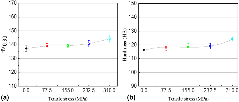
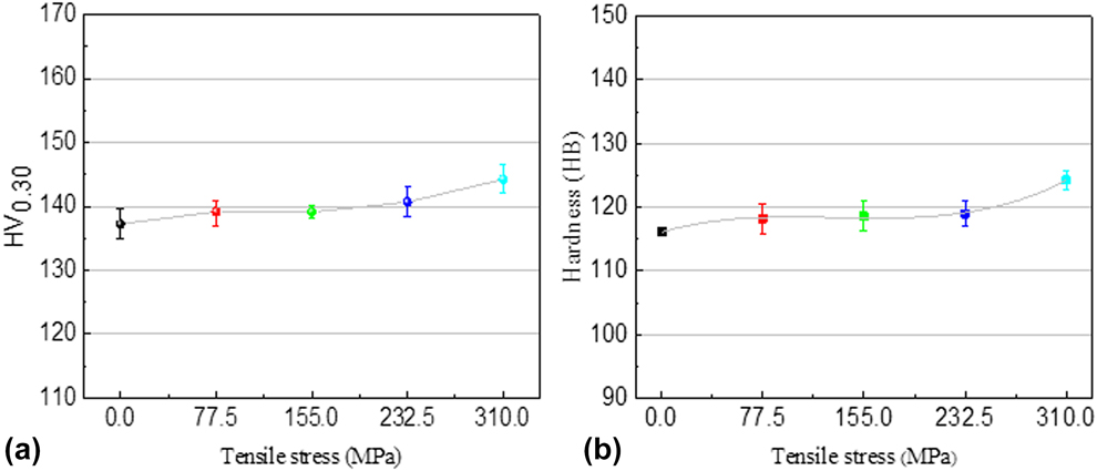
Figure 8 shows the microhardness changes of mild steel specimen after stretched to several different stresses. The microhardness of the original mild steel specimen at the ferrite matrix was about 137 HV, with the increase of the applied stress, the mild steel exhibiting a slight harden, and finally, the microhardness value gets to about 144 HV when the tensile stress increased to its elastic limit. To contrast with the measurement results of lattice parameters and microhardness [Figs. 6(a) and 8(a)], the rise of microhardness could be understood that derived from the effect of the strain-hardening. Besides, the Brinell hardness of the tensile specimen shows the similar fluctuation patterns [see Fig. 8(b)], which also reflects the existence of the microstrain.
The hardness of the mild steel specimen with different tensile stresses. (a) The microhardness of the mild steel specimens. (b) The Brinell hardness of the mild steel specimens.
Conclusions
In summary, a novel application of nonlinear ultrasonic technique to characterize the microstrain in the metal subjected to elastic loading was explored successfully. The conclusions are drawn as follows:
(1) The residual strain increases with increasing applied stress in the mild steel specimen and reaches a maximum 0.036% when the stress gets to its elastic limit.
(2) The nonlinear parameter gradually increases as the applied stress. To compare with the original specimen, the nonlinear parameter of tensile specimen has risen more than 40% at its elastic limit.
(3) From the microstructural analysis, it can be found that the microvoids in tensile specimens were physically small, and no obvious change has been found in the dislocation substructure, which indicates that the β′ change in mild steel within elastic range did not rely so much on the factor of void and dislocation contribution.
(4) The higher sensitivity of the nonlinear measurements to the microresidual strain was demonstrated when the nonlinear parameter value was compared against the results obtained from the traditional measurement of longitudinal wave velocity.
Experimental procedure
Material preparation
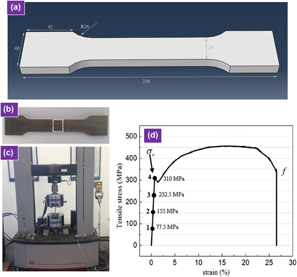
The materials used in this research were the commercial mild steel, with a thickness of 10 mm. The chemical composition of this steel was as follows: C: 0.211, Mn: 0.208, Si: 0.147, Cr: 0.0178, Al: 0.0025, Sn: 0.0022, V: 0.0010, Co: 0.037, P: 0.0148, and Fe: Bal (mass, %). The specimens were machined into the dog-bone-shaped with nominal dimensions of 236 mm (length) × 40 mm (width), which is shown in Fig. 9(a). The elastic limit of this mild steel is 310 MPa. In order to obtain several different levels of residual strain within the range of elasticity, these specimens were stretched to four different applied stresses (using the MTS-C45 tensile testing machine), which is equivalent to 25%, 50%, 75%, and 100% of its elastic limit, respectively (i.e., 77.5 MPa, 155 MPa, 232.5 MPa, and 310 MPa), and the corresponding tensile strain values are 0.18%, 0.35%, 0.51%, and 0.7%, respectively [see Figs. 9(c) and 9(d)].
Diagram of experimental scheme. (a) The dimensions of the tensile sample (all dimensions are in mm). (b) The tensile specimen. (c) The MTS-C45 tensile testing machine. (d) The stress–strain curve and the tensile point of mild steel specimen.

Nonlinear ultrasonic measurement
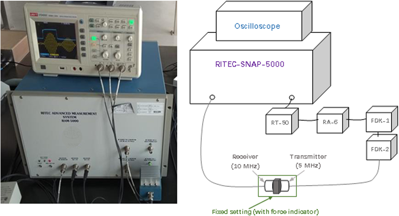
After the tensile experiments, the specimens were cut along the white dashed frames [see Fig. 9(b)] for processing the small pieces with a size of 20 mm (length) × 25 mm (width) ×10 mm (thickness). The RITEC-SNAP-5000 nonlinear system was used in this research for nonlinear ultrasonic measurements. The device contains a valve control amplifier for modulating RF pulse, three precise direct digital synthesizers for high-resolution frequency regulation, and a couple of integrators to process the information that derived from the super-heterodyne phase sensitive receiver. These components could be used to handle the characteristics of ultrasonic emission signal. Besides, outside the RITEC-SNAP-5000, the device was connected to a 50 Ω termination (RT-50), a 6-dB attenuator (RA-6), and two diplexers (FDK-X) for wave filtering (see Fig. 10). The drive voltage is 450 V.
The schematic diagram of the nonlinear ultrasonic measurement.

A pair of transducers was placed on either side of the mild steel specimens. A 5 MHz piezoelectric transducer (SIUI, Φ10, SIUI-Shantou city, China) was used as the transmitter for sending impulses (setting as 10 cycles in this experiment), and a 10 MHz piezoelectric transducer (SIUI, Φ10) was used as the receiver for receiving the fundamental wave (A 1) and second-order harmonic wave signal (A 2). The bandwidth of the transmitter and receiver transducers is 3.75–6.25 MHz and 7.5–12.5 MHz, respectively. The transducers are coupled with light lubrication oil. The scanning frequency was set from 4 to 12 MHz. After conducting the fast Fourier transfer (FFT), the frequency spectrum of transmitted signal can be obtained. Then, the amplitude of A 1 and A 2 can be measured. In addition, to improve the measure accuracy, fixed setting with force indicator was placed, and then the force acted on the transducers can be ensured to be consistent (11.76 N) during each measurement. Besides, for comparison, the CTS1002 (SHANTOU) ultrasonic apparatus was also used to accomplish the traditional longitudinal wave velocity measurements.
Characterization
For examination of the microresidual strain, tensile specimens were fabricated into the small pieces for XRD (Cu Kα radiation) analysis, and the scan range of the X-ray diffraction is set from 40 to 70°, with a rate of 2°/min (Shimadzu-XRD6000, Shimadzu, Japan). Subsequently, the small pieces were etched using 4% nitric acid for microstructure observations using a scanning electron microscope (SEM-EVO18, Jena, Germany). In order to observe the change of dislocation structure after the elastic tensile, the small pieces were also examined by transmission electron microscope (TEM-JEM2100F, Tokyo, Japan); the thin foils were prepared by twin jet polishing in a solution of 10% perchloric acid in methanol at −40 °C at a voltage of 40 V. For assessment of the mechanical property of the mild steel specimens, microhardness and the Brinell hardness values were also measured after the tensile test.
Acknowledgments
The authors would like to express their gratitude for projects supported by the National Natural Science Foundation of China and Macau Science and Technology Development Joint Fund (NSFC-FDCT) (No. 71861167002).