2.1. Notation

Let d be a positive integer. We let $\mathcal{B}$ denote the $\sigma$ -field of Borel sets on $\mathbb{R}^d$ and let $\mathcal{B}_b$ denote its subset of bounded Borel sets. More generally, for any topological space E, we let $\mathcal{B}(E)$ denote its Borel $\sigma$ -field, B(E) its set of measurable bounded real-valued functions, $\overline{E}$ its closure, and $\partial E$ its boundary.

Let $\mathfrak{M}$ be the set of locally finite measures on $(\mathbb{R}^d,\mathcal{B})$ and let $\mathfrak{N}=\{\mu\in\mathfrak{M};\, \text{{for all} } B \in \mathcal{B}_b$ , $\mu(B) \in \mathbb{N}\}$ be the set of locally finite point measures. Note that any $\mu$ in $\mathfrak{N}$ can be expressed as a (possibly infinite) sum of Dirac distributions; the Dirac distribution with point mass at x, for x in $\mathbb{R}^d$ , will be denoted by $\delta_x$ .

Let $C_c(\mathbb{R}^d)$ be the set of continuous real-valued functions with compact support on $\mathbb{R}^d$ . For any measure $\mu\in\mathfrak{M}$ and function $f\in C_c(\mathbb{R}^d)$ , set

\begin{equation*}\mu f \,:\!= \int_{\mathbb{R}^d} f(x) \mu({\text{d}} x).\end{equation*}

We endow $\mathfrak{M}$ with the vague topology. Recall that the vague convergence for a sequence of measures $(\mu_n)_n\subset \mathfrak{M}$ to a measure $\mu\in\mathfrak{M}$ is defined by

\begin{equation*}\mu_nf\xrightarrow[n\rightarrow \infty]{} \mu f\quad \text{{for all} } f\in C_c(\mathbb{R}^d).\end{equation*}

We denote it by

\begin{equation*}\mu_n \xrightarrow[n\rightarrow \infty]{v} \mu .\end{equation*}

It is easily seen that that $\mathfrak{N}$ is a closed subset of $\mathfrak{M}$ for the vague topology.

For any real numbers a and b, $a \vee b$ and $a \wedge b$ denote the maximum and minimum respectively between a and b.

2.2. State space of measure-valued PDMPs

Let K be a finite set called the modes or regimes space. For any mode $v \in K$ , let $E_v$ be an open subset of $\mathfrak{M}$ , representing the state space in mode v. The global state space is then

\begin{equation*}E=\{(v,\zeta) \in K \times \mathfrak{M} \mid v\in K, \zeta \in E_v \}.\end{equation*}

We endow this set E with the $\sigma$ -field $\mathcal{E}$ generated by sets of the form $A=\{v\}\times A_v$ for all Borel sets $A_v\in \mathcal{B}(E_v)$ . For instance, if one can consider the temporal evolution of a cell population characterized by state variables such as age, size, growth, maturity, or protein content, then the quantity $\zeta\in \mathfrak{N}$ represents such state variables and the mode can be the experiment conditions. In the following example, we consider a simple case with only one mode and where the variable state corresponds to the cell size.

Example 2.1. Consider a population of three individuals at a given time. Their sizes are denoted by $(x_i)_{1\leqslant i \leqslant 3}$ . This population is identified with the measure

\begin{equation*} \zeta=\sum_{i=1}^3 \delta_{x_i} \in \mathfrak{N}. \end{equation*}

It gives a complete view of the population: all the information is contained in $\zeta$ . As time goes by, the number of individuals may increase or decrease, leading to more or fewer terms in this Dirac sum representation, but it will remain a measure in $\mathfrak{N}$ . This representation is then easier to manipulate than a changing-dimension vector.

On the measure space $\mathfrak{M}$ , we introduce a particular metric $\rho$ for the vague topology in order to have a Polish space (i.e. a separable completely metrizable topological space). This property will be used in Section 2.3 for the explicit construction of the stochastic process. As shown in [Reference Kallenberg17, Appendix], a suitable choice for $\rho$ is constructed as follows. Let $\mathcal{C}$ be a countable basis of open bounded subsets in $\mathbb{R}^d$ closed under finite unions. For all C in $\mathcal{C}$ , there exists a sequence $(C_n)_n$ in $\mathcal{B}_b$ and an increasing sequence $(\kern1.3ptf_{C,n})_n$ in $C_c(\mathbb{R}^d)$ such that

\begin{equation*}f_{C,n} \xrightarrow[n\rightarrow \infty]{} \mathds{1}_C \quad\text{and}\quad\mathds{1}_{C_n}\leqslant f_{C,n}\leqslant\mathds{1}_{C}.\end{equation*}

Since $\mathcal{C}$ is countable, the set $\{f_{C,n} | C\in\mathcal{C}$ , $n\in\mathbb{N}\}$ is also countable, and we then number those functions $f_1,f_2,\ldots.$ Any measure $\mu$ is completely determined by the set $\{ \mu f_k, k\in\mathbb{N}\}$ . Now, for all $\mu$ and $\mu'$ in $\mathfrak{M}$ , we define the distance $\rho$ by

\begin{equation*} \rho(\mu,\mu')\,:\!= \sum_{k\geqslant1}\frac{1}{2^k} ( 1-\exp({-}|\mu f_k-\mu' f_k|)). \end{equation*}

From this metric on $\mathfrak{M}$ , we define a metric on E related to its hybrid structure: any two points in E with different modes must be arbitrarily far away from each other. For all $x=(v,\zeta)$ and $x'=(v',\zeta')$ in E, set

\begin{equation*} \rho_0(x,x')\,:\!= \begin{cases} { \dfrac{2}{\pi} \arctan(\rho(\zeta,\zeta'))} &\text{if $ v= v'$,}\\[10pt] 1 &\text{otherwise}.\end{cases} \end{equation*}

Thus $\rho_0(x,x')$ equals 1 if and only if x and xʹ have different modes. With this metric, a sequence $(x_n)_n=(v_n,\zeta_n)_n$ converges to $x=(v,\zeta)$ in $(E,\rho_0)$ if and only if there exists some m in $\mathbb{N}$ such that

\begin{equation*} \begin{cases}v_n=v \text{ for }n\geqslant m, \\[5pt] \zeta_{m+k} \xrightarrow[k\rightarrow \infty]{} \zeta \text{ in } (E_v,\rho).\end{cases}\end{equation*}

We have

\begin{equation*}\overline{E}=\{(v,\zeta) \in K \times \mathfrak{M} \mid v\in K, \zeta \in \overline{E}_v \},\end{equation*}

the closure of E for the distance $\rho_0$ . The following statement is then straightforward.

2.3. Construction of measure-valued PDMPs

We now introduce the three local characteristics of the PDMP specifying the dynamics of trajectories between jumps, the jump times, and the post-jump locations.

1. • The flow $\Phi$ is defined by $(x,t) \mapsto \Phi(x,t)=(v,\Phi_v(\zeta,t))$ for all $x=(v,\zeta)$ in E and non-negative t, where the functions $\Phi_v\colon \mathfrak{M}\times \mathbb{R}\rightarrow \mathfrak{M}$ are continuous and have a semi-group property: for all $s,t \geqslant0$ , we have $\Phi_v(\cdot,t+s)=\Phi_v(\Phi_v(\cdot,s),t)$ . The flow describes the deterministic trajectory of the process between jumps. Let

   \begin{equation*}t^*(x)=\inf\{t>0, \Phi_v(t,\zeta)\in \partial E_v\}\end{equation*}
   be the deterministic time the flow takes to reach the boundary of the domain starting from $x=(v,\zeta)\in E$ , with the usual convention $\inf\emptyset=+\infty$ . An infinite exit time $t^*$ means that the process cannot reach the boundary in finite time.

2. • The jump intensity $\lambda\colon E \rightarrow \mathbb{R}_+$ is a measurable function, with a local integrability property: for all $x=(v,\zeta)\in E$ there exists some $\varepsilon>0$ such that

   \begin{equation*}\int_0^\varepsilon \lambda(v,\Phi_v(\zeta,s)) \,{\text{d}} s <\infty.\end{equation*}
   It determines the frequency of the jumps.

3. • The Markov kernel $\mathcal{Q}\colon \overline{E} \times \mathcal{B}(E) \rightarrow [0,1]$ selects the post-jump locations. It has the following property:

   \begin{equation*} Q(x,\{x\})=0\quad{\text{for all } x\in E}, \end{equation*}
   meaning that the process cannot have a no-move jump.

From these local characteristics, one can construct a stochastic process similarly to [Reference Davis10, Section 24] as follows. Let $(\Omega,\mathcal{F},\mathbb{P})$ be the canonical space for a sequence $(U_n)_{n\geqslant 1}$ of independent random variables with uniform distribution on [0, 1]. The sample path of an E-valued PDMP $(X_t(\omega))_{t\geqslant 0}$ starting from a fixed initial point $x=(v,\zeta)\in E$ and for some $\omega\in \Omega$ is defined iteratively. Let

(2.1) \begin{equation}F(x,t)=\mathds{1}_{\{t<t^*(x)\}} \exp\biggl({-}\int_0^t \lambda(v,\Phi_v(\zeta,s))\,{\text{d}} s\biggr)\end{equation}

for $(x,t)=(v,\zeta,t)\in E\times\mathbb{R}_+$ , let $ \Psi_1$ be the function from $E\times [0,1]$ onto $\mathbb{R}_+$ defined by

\begin{equation*} \Psi_1(x,u)=\inf\{t\geqslant 0;\ F(x,t)\leqslant u\},\end{equation*}

and let $S_1(\omega)=T_1(\omega)= \Psi_1(x,U_1(\omega))$ be the first jump time of the process. Thus $F(x,\cdot)$ is the survivor function of $T_1$ .

As the spaces $\mathfrak{M}$ and $\overline{E}$ are Polish, one can use [Reference Kolokoltsov18, p. 6] to obtain that $\{\mathcal{Q}(x,\cdot) \}_{x\in \overline{E}}$ is a collection of probability measures on $\overline{E}$ , with a measurable dependence on the parameter x in $\overline{E}$ . Then there is a measurable function $\Psi_2\colon E\times [0,1]\rightarrow E$ such that the distribution of $\Psi_2(y,U)$ is $\mathcal{Q}(y,\cdot)$ for any random variable U with uniform distribution on [0, 1]. Hence one can then define

\begin{align*}X_t(\omega)&=\Phi_v(\zeta,t),\quad \text{ for } 0\leqslant t<T_1, \\*X_{T_1}(\omega)&=\Psi_2 ((v,\Phi_v(\zeta,T_1(\omega))),U_2(\omega)).\end{align*}

Hence the trajectory $X_t$ follows the deterministic flow starting from $X_0=x$ until the first jump time $T_1$ . At $T_1$ a new location $Z_1=X_{T_1}$ is drawn according to the Markov kernel $\mathcal{Q}$ . Namely, the law $\mathcal{L}(Z_1 \mid T_1)$ of $Z_1$ conditionally on $T_1$ is

\begin{equation*} \mathcal{L}(Z_1 \mid T_1)= \mathcal{Q}(\Phi(x,S_1),\cdot).\end{equation*}

The process now restarts from $X_{T_1}$ following the same steps. Define

\begin{equation*}S_2(\omega)= \Psi_1(X_{T_1}(\omega),U_3(\omega)),\quad T_2(\omega)=S_1(\omega)+S_2(\omega),\end{equation*}

and set

\begin{align*}X_t(\omega)&=\Phi(X_{T_1}(\omega),t-T_1(\omega)),\quad \text{ for } T_1(\omega)\leqslant t<T_2(\omega),\\*X_{T_2}(\omega)&=\Psi_2 ((v,\Phi(X_{T_1}(\omega),S_2(\omega))),U_4(\omega)),\end{align*}

and so on. In order to avoid explosion issues, the following assumption will hold throughout the paper.

Assumption 2.1. For all (x,t) in $E\times \mathbb{R}_+$ ,

\begin{equation*} \mathbb{E}_x \Biggl[\sum_{n=1}^{\infty} \mathds{1}_{(T_n<t})\Biggr] < \infty.\end{equation*}

Hence the trajectories of $(X_t)$ are well-defined for all $t\geqslant 0$ .

The positive random variables $S_1,S_2,\ldots$ are the times between two consecutive jumps or inter-jump times. For notational convenience, we set $T_0=S_0=0$ and $T_n\,:\!=\sum_{i=1}^n S_n$ the nth jump time of the process. Note that we have $T_1=S_1$ and $S_{n+1}=T_{n+1}-T_n$ . The sequence $(Z_n)_n$ with $Z_n=X_{T_n}$ describes the post jump locations of the process. By construction, all the randomness of the continuous-time process $(X_t)_{t\geqslant 0}$ is contained in the discrete-time process $(Z_n,S_n)_{n\geqslant 0}$ .

2.4. Structure of stopping times and Markov property

The aim of this section is to prove that the special structure of stopping times for finite-dimensional PDMPs given in [Reference Davis10, Theorem A2.3] still holds in the measure space context. This yields the Markov property and will be important for the study of the optimal stopping problem in Section 3.

Let $D_E[0,+\infty)$ be the set of functions on $\mathbb{R}_+$ with values in E that are right-continuous with left limits. Let $\tilde X_t$ denote the coordinate function $\tilde X_t(\kern1.3ptf)=f(t)$ for $f\in D_E[0,+\infty)$ . Let $(\mathcal{F}_t^0)_{t\geqslant 0}$ denote the natural filtration of $(\tilde x_t)$ and $\mathcal F^0=\vee_{t\geqslant 0}\mathcal F^0_t$ . Under Assumption 2.1, for each starting point $x\in E$ , the construction in the previous section defines a measurable mapping $\Psi_x$ from $\Omega$ onto $D_E[0,+\infty)$ such that $\tilde X_t(\Psi_x(\omega))=X_t(\omega)$ . Let $\mathbb P_x$ denote the image measure of $\mathbb P$ by $\Psi_x$ . This defines a family of measures $(\mathbb P_x)_{x\in E}$ on $D_E[0,+\infty)$ . We shall identify $\tilde X_t$ and $X_t$ . For any probability measure $\nu$ on E, define the measure $\mathbb P_\nu$ on $(D_E[0,+\infty),\mathcal F^0)$ by $\mathbb P_\nu(\cdots)=\int_E\mathbb P_x(\cdot)\nu({\text{d}} x)$ . Now let $\mathcal{F}_t^\nu$ be the completion of $\mathcal{F}_t^0$ with all $\mathbb P_\nu$ -null sets of $\mathcal{F}^0$ and define $\mathcal{F}_t=\cap_{\nu\in\mathcal{P}(E)}\mathcal{F}_t^\nu$ , where $\mathcal{P}(E)$ is the set of probability measures on E.

We can now state a crucial result on the structure of stopping times for our process.

Theorem 2.1. A non-negative random variable $\tau$ is a $(\mathcal{F}_t)_{t\geqslant 0}$ stopping time if and only if there exists a sequence $(R_n)_{n\in \mathbb N}$ of non-negative $(\mathcal{F}_{T_n})_{n\in \mathbb N}$ -adapted random variables such that

\begin{equation*}\tau=\sum_{n=1}^\infty R_{n-1}\wedge S_n.\end{equation*}

Proof. The proof follows the same lines as in [Reference de Saporta, Dufour and Zhang11, Section 1.7]. It is based on Theorem A2.3 in [Reference Davis10], which is valid for any right-continuous piecewise constant process taking values in a Borel set and the one-to-one correspondence between our process $(X_t)$ and the right-continuous piecewise constant $E\times\mathbb N$ -valued process $(\eta_t)$ defined by

\begin{equation*}\eta_t=(X_0,0), \ t<T_1,\quad \eta_t=(X_{T_n},n),\ T_n\leqslant t < T_{n+1}\end{equation*}

(see [Reference Davis10, (25.1)]).□

Proof. The strong Markov property is proved in the same way as in [Reference Davis10, Section 25], using Theorem 2.1 and the one-to-one correspondence with the piecewise constant process $(\eta_t)$ defined above.□

2.5. Toy example

We now develop Example 2.1 into a more generic model for some cells population. Typically, cells grow and divide into two daughter cells that start growing and then divide and so on.

2.5.2 Population model

We now consider the previous cell growth-division dynamics but for the whole population instead of a single randomly selected cell. Again we consider a single mode so that the space E is simply $\mathfrak{N}$ .

Let $\zeta=\sum_{i=1}^n \delta_{x_i}$ be in $\mathfrak{N}$ be an initial state of n cells with respective sizes $(x_i)_{1\leqslant i\leqslant n}$ . Each cell grows following the previous dynamics, so that globally the flow is

\begin{equation*} \begin{array}{c@{\,}c@{\,}c@{\ }c@{\ }c}{{\Phi}} & : & {\mathfrak{N}\times\mathbb{R}_+} & \to & {\mathfrak{N}}\\ & & {(\zeta,t)} & \mapsto & {\sum_{i=1}^n \delta_{\phi(x_i,t)}.}\\\end{array} \end{equation*}

The first jump time corresponds to the first splitting, i.e. the minimum between n exponentially distributed random variables. Thus the jump intensity is

\begin{equation*} \begin{array}{c@{\,}c@{\,}c@{\ }c@{\ }c}{\lambda} & : & \mathfrak{N} & \to & \mathbb{R} \\ & & \zeta& \mapsto & \sum_{i=1}^n l(x_i).\\\end{array} \end{equation*}

Given that the jth cell is the one that splits, the post-jump location is

\begin{equation*}Z_1=\sum_{\substack{ i=1\\i\neq j}}^n \delta_{x_i}+2 \delta_{x_j/2}, \end{equation*}

where cell number j was removed and two new cells are added with half the size of cell j. For notational convenience, we set

\begin{equation*}\zeta_{(j)}\,:\!=\zeta-\delta_{x_j}+2 \delta_{x_j/2}. \end{equation*}

Thus, for A in $\mathcal{E}$ , the Markov jump kernel of the PDMP is given by

\begin{equation*} {\mathcal{Q}}(\zeta,A)=\sum_{j=1}^n \frac{l(x_j)}{\sum_{i=1}^n l(x_i)} \mathds{1}_A(\zeta_{(j)}). \end{equation*}

2.5.3. Time-augmented population model

Sometimes it is convenient to add time in the state variable of a PDMP, for instance if we want to use time-dependent jump intensity, or trigger some jump when a certain lapse of time has passed, or to study control problems with time-dependent reward functions. In [Reference Davis10, Section 31] Davis proves that for finite-dimensional PDMPs, the time-augmented process is still a PDMP. The same property holds in the framework of our toy example.

We consider the time-augmented process $(\widetilde{X}_t)_{t}$ defined as the PDMP on $\mathfrak{N}$ starting from the initial state 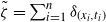$\tilde\zeta=\sum_{i=1}^n \delta_{(x_i,t_i)}$ . The flow is now given by

\begin{equation*} \begin{array}{c@{\,}c@{\,}c@{\ }c@{\ }c}{{\widetilde{\Phi}}} & : & {\mathfrak{N}\times\mathbb{R}_+} & \to & {\mathfrak{N}}\\ & & {(\tilde\zeta,t)} & \mapsto & {\sum_{i=1}^n \delta_{(\phi(x_i,t), t_i+t)},}\\\end{array} \end{equation*}

for any $\tilde\zeta$ in $\mathfrak{N}$ of the form 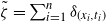$\tilde\zeta=\sum_{i=1}^n \delta_{(x_i,t_i)}$ . The jump intensity is

\begin{align*}\begin{array}{c@{\,}c@{\,}c@{\ }c@{\ }c} {\widetilde{\lambda}} & : & \mathfrak{N} & \to & \mathbb{R} \\ & & \tilde\zeta=\sum_{i=1}^n \delta_{(x_i,t_i)}& \mapsto & \sum_{i=1}^n l(x_i),\\ \end{array}\end{align*}

and the jump kernel is simply

\begin{equation*}\widetilde{\mathcal{Q}}\Biggl(\sum_{i=1}^n \delta_{(x_i,t_i)},A\Biggr)=\sum_{j=1}^n \frac{l(x_j)}{\sum_{i=1}^n l(x_i)} \mathds{1}_A \Biggl(\sum_{i=1}^n \delta_{(x_i,t_i)}-\delta_{(x_j,t_i)}+2\delta_{(x_j/2,t_i)}\Biggr).\end{equation*}

Remark 2.1. Following the definition of the time-augmented process by Davis, we could have defined the measure-valued time-augmented process on $\mathfrak{N}\times\mathbb{R}_+$ with the flow

\begin{equation*}\Biggl(\sum_{i=1}^n\delta_{x_i},u\Biggr)\to\Biggl(\sum_{i=1}^n\delta_{\phi_{u,t}(x_i)},u+t\Biggr).\end{equation*}

But formally PDMPs on product spaces such as $\mathfrak{N}\times\mathbb{R}_+$ are not included in our previous construction. However, in our main examples, we only consider $\tilde\zeta$ in the form $\sum_{i=1}^n \delta_{(x_i,u)}$ which roughly means that all cells have the same current time.

We will further study this toy example in Section 4 to prove that controlling the whole population is not equivalent to controlling a suitably chosen random lineage.

3.1. Dynamic programming operators

We start with some additional notation and assumption. For w in B(E), x in E, and l a measurable real-valued function on E, we denote for short

\begin{equation*}l\mathcal{Q} w (x) \,:\!= l(x)\times \mathcal{Q} w(x)=l(x)\int_E w(y) \mathcal{Q} (x,{\text{d}} y). \end{equation*}

The following assumption is made for simplicity reasons. It is satisfied in most real-life examples, for instance when monitoring a population until some finite horizon time.

We now define some operators on B(E). Let $\textbf{H}$ be the operator from $B(\overline{E})$ onto $B(\overline{E}\times \mathbb{R}_ +)$ defined for all h in $B(\overline{E})$ , x in $\overline{E}$ and $t\in\mathbb{R}_+$ , by

\begin{equation*}\textbf{H} h(x,t) = h (\Phi(x,t\wedge t^*(x))) \,\text{e}^{-\Lambda(x,t\wedge t^*(x))}, \end{equation*}

and let $\textbf{I}$ be the operator from B(E) onto $B(E\times \mathbb{R}_ +)$ defined for all w in B(E), x in E, and $t\in\mathbb{R}_+$ , by

\begin{equation*}{\textbf{I}}{w}(x,t) =\int_0^{t\wedge t^*(x)}\lambda\mathcal{Q} w(\Phi(x,s)) \,\text{e}^{-\Lambda(x,s)}\,\text{d}s, \end{equation*}

where

\begin{equation*}\Lambda(x,t)=\int_0^t \lambda (\Phi(x,s))\,{\text{d}} s. \end{equation*}

We also introduce operator $\textbf{K}$ from B(E) onto B(E), defined for all w in B(E) and x in E as

\begin{equation*} {\textbf{K}}{w}(x)= \int_0^{t^*(x)}\lambda\mathcal{Q} w(\Phi(x,s)) \,\text{e}^{-\Lambda(x,s)}\text{d}s + \mathcal{Q} w (\Phi(x,t^*(x))) \,\text{e}^{-\Lambda(x,t^*(x))}. \end{equation*}

It is straightforward to see that these operators can be expressed as expectations involving the embedded Markov chain $(Z_n,S_n)$ defined in Section 2.3.

Proposition 3.1. For all h in $B(\overline{E})$ and w in B(E), x in E and $t\geqslant 0$ , we have

\begin{align*}\textbf{H} h(x,t) &= \mathbb{E}_x [h(X_{t\wedge t^*(x)})\,\mathds{1}_{S_1> t\wedge t^*(x)}]=h (\Phi(x,t\wedge t^*(x)) ) \mathbb{P}_{x} (S_1>t\wedge t^*(x)),\\*\textbf{I} w(x,t) &= \mathbb{E}_x [ w(Z_1)\mathds{1}_{S_1 \leqslant t\wedge t^*(x)} ],\\*\textbf{K} w(x)&=\mathbb{E}_x[w(Z_1)].\end{align*}

Finally we let $\textbf{J}$ and $\textbf{L}$ denote the operators from $B(E) \times B(\overline{E})$ onto $B(E\times\mathbb R_+)$ and B(E) respectively defined for all w in B(E), h in $B(\overline{E})$ , x in E, and $t\in\mathbb{R}_+$ , by

\begin{align*}\textbf{J}(w,h)(x,t)&= \textbf{H} h(x,t)+\textbf{I} w(x,t),\\*\textbf{L}(w,h)(x)&= \sup_{t\geqslant 0} \{ \textbf{J}(w,h)(x,t) \} \vee \textbf{K} w (x). \end{align*}

We can now propose an iterative construction of value functions by iterating operator $\textbf{L}$ . For all $x\in E$ , set

\begin{align*} \mathbb{V}_{0}(x)&=g(x), \\*\mathbb{V}_{n}(x)&=\textbf{L}(\mathbb{V}_{n-1},g)(x) \quad \text{for all }n \geqslant 1,\end{align*}

where g is the reward function of the optimal stopping problem. Clearly the functions $\mathbb{V}_{n}$ are in B(E). Roughly speaking, operator $\textbf{L}$ represents the best compromise between stopping at the best location along the deterministic trajectory following the flow ( $ \sup_{t\geqslant 0} \textbf{J}$ part) or waiting until the next jump ( $\textbf{K}$ part).

3.2. Family of stopping times

Now we introduce a family of random variables and prove they are stopping times. They will be candidate $\varepsilon$ -optimal stopping times for our optimal stopping problem. For all $x\in E$ , $n\in\mathbb{N}$ , and $\varepsilon>0$ , set

\begin{equation*}r_{n,\varepsilon}(x)=\begin{cases} t^*(x)\quad \text{if }\textbf{K}\mathbb{V}_{n}(x)> \sup_{t>0}\textbf{J}(\mathbb{V}_{n},g)(x,t), \\[5pt] \inf\{s\geqslant0;\,\textbf{J}(\mathbb{V}_{n},g)(x,s)\geqslant\sup_{t>0}\textbf{J}(\mathbb{V}_{n},g)(x,t)-\varepsilon \} \quad \text{otherwise.} \end{cases}\end{equation*}

For all $\varepsilon>0$ and $n\geqslant 2$ , also set

\begin{align*}R_{1,\varepsilon}&=r_{0,\varepsilon}(Z_0),\\[2pt] R_{n,0}^\varepsilon&=r_{n-1,\varepsilon/2}(Z_0),\\[2pt] R_{n,k}^\varepsilon&=r_{n-k-1,\varepsilon/2^{k}}(Z_k)\mathds{1}_{(R_{n,k-1}^\varepsilon\geqslant S_k)}, \quad 1\leqslant k\leqslant n-1.\end{align*}

Then $R_{n,k}^\varepsilon$ is clearly $\mathcal F_{T_k}$ -measurable for $0\leqslant k\leqslant n-1$ . Finally, define $S_{1,\varepsilon}\,:\!=r_{0,\varepsilon}(Z_0)\wedge T_1=R_{1,0}^\varepsilon\wedge S_1$ , and by iteration,

\begin{equation*}S_{n,\varepsilon}\,:\!=\begin{cases}R_{n,0}^{\varepsilon} &\text{if $T_1>R_{n,0}^{\varepsilon} $,}\\[5pt] T_1+\theta(T_1)S_{n-1,\varepsilon/2} &\text{else $ T_1\leqslant R_{n,0}^{\varepsilon}$,}\end{cases}\end{equation*}

where $\theta(t)$ is the shift operator with lag t on $D_E[0,+\infty)$ , namely for $f\in D_E[0,+\infty)$ , $\theta(t)f(\cdot)=f(t+\cdot)$ .

In order to prove that the $S_{n,\varepsilon}$ are stopping times in $\mathcal M_n$ , we first study the effect of the shift operator on $R_{n,k}^\varepsilon$ .

Lemma 3.1. For all $\varepsilon>0$ and $n\geqslant 2$ and $1\leqslant k\leqslant n-1$ , on the set $(T_1\leqslant S_{n,2\varepsilon})$ , we have

\begin{equation*}R_{n,k}^{2\varepsilon}=\theta(T_1)(R_{n-1,k-1}^\varepsilon).\end{equation*}

Proof. For $n=2$ , by definition, we have $R_{1,0}^\varepsilon=r_{0,\varepsilon}(Z_0)$ and hence $\theta(T_1)(R_{1,0}^\varepsilon)=r_{0,\varepsilon}(Z_1)$ and $R_{2,1}^{2\varepsilon}=r_{0,\varepsilon}(Z_1)$ on $(T_1\leqslant S_{2,2\varepsilon})=(T_1\leqslant R_{2,0}^\varepsilon)$ . Hence the result holds.

For $n\geqslant 3$ , we prove the result by induction on k using similar arguments and the fact that $(T_1\leqslant S_{n,\varepsilon})=(R_{n,0}^{2\varepsilon}\geqslant T_1)$ .□

We now prove that $S_{n,\varepsilon}$ is a stopping time using the characterization of Theorem 2.1.

Lemma 3.2. For all $\varepsilon>0$ and $n\in\mathbb N^*$ , we have

\begin{equation*}S_{n,\varepsilon}=\sum_{k=1}^n R_{n,k-1}^\varepsilon\wedge S_k.\end{equation*}

In particular, $S_{n,\varepsilon}$ is a stopping time and $S_{n,\varepsilon}\leqslant T_n$ .

Proof. We proceed by induction on n. For $n=1$ , by definition, $S_{1,\varepsilon}=r_{0,\varepsilon}(Z_0)\wedge T_1=R_{1,k-1}^\varepsilon\wedge S_1$ and the result is true.

Suppose the result holds for $n-1$ . From the definition, on the event

\begin{equation*}(r_{n-1,\varepsilon/2}(Z_0)=R_{n,0}^\varepsilon<S_1),\end{equation*}

we have $S_{n,\varepsilon}=R_{n,0}^\varepsilon$ and $R_{n,1}^\varepsilon=0<S_2$ , $R_{n,2}^\varepsilon=0<S_3$ , and so on, so that $\sum_{k=1}^n R_{n,k-1}^\varepsilon\wedge S_k=R_{n,0}^\varepsilon$ and the result is valid.

On the event $(R_{n,0}^\varepsilon\geqslant S_1)$ , by definition $S_{n,\varepsilon}=T_1+\theta(T_1)S_{n-1,\varepsilon/2}$ . Now, the induction hypothesis and the previous lemma yield

\begin{equation*}T_1+\theta(T_1)S_{n-1,\varepsilon/2}=S_1+\sum_{k=1}^{n-1} R_{n,k}^{\varepsilon}\wedge S_{k+1}=\sum_{k=1}^n R_{n,k-1}^\varepsilon\wedge S_k,\end{equation*}

on $(R_{n,0}^\varepsilon\geqslant S_1)$ . Hence the result.□

3.3. Characterization of the value function

We can now state and prove our main result, namely that the value function $\mathbb{V}$ of the optimal stopping problem (3.1) equals the Nth iterate $\mathbb{V}_{N}$ and that $S_{N,\varepsilon}$ is an $\varepsilon$ -optimal stopping time.

Theorem 3.1. Let x be in E and $n\in \mathbb{N}$ . Then, for all $\varepsilon>0$ , $S_{n,\varepsilon}$ is a stopping time in $\mathcal{M}_n$ and

(3.2) \begin{align}\equationnumber{\normalfont(3.2)}\mathbb{V}_{n}(x)&=\sup_{S\in \mathcal{M}_n}\mathbb{E}_{x}[g(X_S)], \end{align}

(3.3) \begin{align}\equationnumber{\normalfont(3.3)}\mathbb{E}_{x}[g(X_{S_{n,\varepsilon}})]&\geqslant \mathbb{V}_{n}(x)-\varepsilon. \end{align}

Proof. By an induction argument we will prove equation (3.3) and the following inequality:

(3.4) \begin{equation}\mathbb{E}_{x}[g(X_{S\wedge T_n})] \leqslant \mathbb{V}_{n}(x)\quad {\text{for all } S \in \mathcal{M},\ n\in\mathbb{N}.}\end{equation}

These two equations imply (3.2). Indeed, for all S in $\mathcal{M}_{\infty}$ , we have $S\wedge T_n \in \mathcal{M}_n$ ; then, for all S in $\mathcal{M}_{\infty}$ , n in $\mathbb{N}$ and x in E, (3.3) and (3.4) yield

\begin{equation*}\mathbb{V}_{n}(x)-\varepsilon \leqslant \mathbb{E}_{x}[g(X_{S_{n,\varepsilon}})] \leqslant \sup_{S\in \mathcal{M}_n} \mathbb{E}_{x}[g(X_{S})] = \sup_{S\in \mathcal{M}_n} \mathbb{E}_{x}[g(X_{S\wedge T_n})] \leqslant \mathbb{V}_{n}(x),\end{equation*}

which is valid for all positive $\varepsilon$ , hence the result.

It remains now to prove (3.4) and (3.3) by induction.

The case $n=1$ is based on Theorem 2.1 Indeed, we obtain

\begin{equation*}\mathbb{E}_{x}[g(X_{S\wedge T_1})] =\mathbb{E}_{x}[g(X_{R_0\wedge T_1})],\end{equation*}

for some $\mathcal{F}_0$ -measurable random variable $R_0$ . From this, we deduce

\begin{align*} \mathbb{E}_{x}[g(X_{S\wedge T_1})] &=\mathbb{E}_{x}[g(X_{R_0})\mathds{1}_{T_1 > R_0}] +\mathbb{E}_{x}[g(Z_1)\mathds{1}_{T_1\leqslant R_0}]\\[4pt] &= \textbf{H} g (x,R_0)+ \textbf{I} g (x,R_0) \\[4pt] &= \textbf{J}(g,g)(x,R_0)\\[4pt] &\leqslant \sup_{t\geqslant 0} \{ \textbf{J}(g,g)(x,t) \}\\[4pt] &\leqslant \mathbb{V}_{1}(x){,} \end{align*}

which proves (3.4) for $n=1$ . To prove (3.3), we distinguish two cases.

1. • If $ \textbf{K} g (x) > \sup_{t\geqslant 0}\textbf{J}(g,g)(x,t) $ , then $\mathbb{V}_{1}(x)=\textbf{K} g(x)=\mathbb{E}_{x}[g(Z_1)]$ and also

   \begin{equation*}S_{1,\varepsilon}=t^*(x) \land T_1=T_1.\end{equation*}
   Thus
   \begin{equation*}\mathbb{E}_{x}[g(X_{S_{1,\varepsilon}})]=\mathbb{E}_{x}[g(Z_1)]=\mathbb{V}_{1}(x)\geqslant \mathbb{V}_{1}(x)-\varepsilon.\end{equation*}

2. • Otherwise, $\mathbb{V}_{1}(x)=\sup_{t\geqslant 0}\textbf{J}(g,g)(x,t)$ and, by definition of $\textbf{J}$ ,

   \begin{align*} \mathbb{E}_{x}[g(X_{S_{1,\varepsilon}})] &=\mathbb{E}_{x}[g(X_{r_{0,\varepsilon}(x)\land T_1})]\\[4pt] &=\mathbb{E}_{x}[g(X_{r_{0,\varepsilon}(x)})\mathds{1}_{T_1 \geqslant r_{0,\varepsilon}(x)}] +\mathbb{E}_{x}[g(Z_1)\mathds{1}_{T_1\leqslant r_{0,\varepsilon}(x)}]\\[4pt] &=\textbf{J}(g,g)(x,r_{0,\varepsilon}(x)).\end{align*}

We then deduce, by definition of $r_{0,\varepsilon}$ ,

\begin{equation*} \mathbb{E}_{x}[g(X_{S_{1,\varepsilon}})] \geqslant \sup_{t\geqslant 0}\{ \textbf{J}(g,g)(x,t)\} -\varepsilon=\mathbb{V}_{1}(\mu)-\varepsilon. \end{equation*}

This completes the proof of (3.3) for $n=1$ .

Now, let $N\geqslant 1$ , suppose that (3.4) and (3.3) hold true for all $n\leqslant N$ , and prove that they hold for $n=N+1$ .

Begin by proving (3.4). Again, this is based on Theorem 2.1 As S is a stopping time, it can be decomposed as

\begin{equation*}S=\sum_{n=1}^\infty R_{n-1}\wedge S_n,\end{equation*}

where $(R_n)_{n\in \mathbb N}$ are non-negative $(\mathcal{F}_{T_n})_{n\in \mathbb N}$ -adapted random variables. In particular, on $(S\geqslant T_1)$ we have

\begin{equation*}S=S_1+\sum_{n=2}^\infty R_{n-1}\wedge S_n=T_1+\theta(T_1)(S'),\end{equation*}

for some stopping time Sʹ. Thus we have

(3.5) \begin{align}\equationnumber{\normalfont(3.5)}\mathbb{E}_{x}[g(X_{S\wedge T_{n+1}})]&= \mathbb{E}_{x}[g(X_{S\wedge T_{1}})\mathds{1}_{S<T_1}]+ \mathbb{E}_{x}[g(X_{S\wedge T_{n+1}})\mathds{1}_{S\geqslant T_1}] \notag\\[5pt] &= \mathbb{E}_{x}[g(X_{R_0\wedge T_{1}})\mathds{1}_{R_0<T_1}]+ \mathbb{E}_{x}[g(X_{S\wedge T_{n+1}})\mathds{1}_{R_0\geqslant T_1}] \notag\\[5pt] &=\mathbb{E}_{x}[g(X_{R_0})\mathds{1}_{R_0<T_1}]+ \mathbb{E}_{x}[\mathbb{E}_{x}[g(X_{(T_1+\theta(T_1)(S'))\wedge T_{n+1}})\vert \mathcal{F}_{1}]\mathds{1}_{R_0\geqslant T_1}]\notag\\[2pt] &=\mathbb{E}_{x}[g(X_{R_0})\mathds{1}_{R_0<T_1}]+ \mathbb{E}_{x}[\mathbb{E}_{Z_1}[g(X_{ S'\wedge T_{n}})]\mathds{1}_{R_0\geqslant T_1}] \end{align}

(3.6) \begin{align}\equationnumber{\normalfont(3.6)}&\leqslant \mathbb{E}_{x}[g(X_{R_0})\mathds{1}_{R_0<T_1}]+ \mathbb{E}_{x}[ \mathbb{V}_{n}(Z_1) \mathds{1}_{R_0\geqslant T_1}] \end{align}

\begin{align}\equationnumber{\normalfont}&\leqslant \sup_{r\geqslant 0} \mathbb{E}_{x}[g(X_{r})\mathds{1}_{r<T_1}]+ \mathbb{E}_{x}[ \mathbb{V}_{n}(Z_1) \mathds{1}_{r\geqslant T_1}] \notag \\ &\leqslant \sup_{r\geqslant 0} \textbf{J} (\mathbb{V}_{n},g)(x,r) \lor \textbf{K} \mathbb{V}_{n}(x) \notag \\ & =\mathbb{V}_{n+1}(x). \notag\end{align}

Line (3.5) is obtained thanks to the strong Markov property. The induction hypothesis is applied in line (3.6). This achieves the induction for (3.4).

Let us now prove (3.3). We have

\begin{align*}\mathbb{E}_{x}[g(X_{S_{n+1,2\varepsilon}})] &=\mathbb{E}_{x}[g(X_{S_{n+1,2\varepsilon}})\mathds{1}_{R_{n,0}^\varepsilon<T_1}]+\mathbb{E}_{x}[g(X_{S_{n+1,2\varepsilon}})\mathds{1}_{R_{n,0}^\varepsilon\geqslant T_1}] \\[3pt] &=\mathbb{E}_{x}[g(X_{R_{n,0}^\varepsilon})\mathds{1}_{R_{n,0}^\varepsilon<T_1}]+\mathbb{E}_{x}[g(X_{T_1+\theta(T_1)S_{n,\varepsilon}})\mathds{1}_{R_{n,0}^\varepsilon\geqslant T_1}] \\[3pt] &=\mathbb{E}_{x}[g(X_{R_{n,0}^\varepsilon})\mathds{1}_{R_{n,0}^\varepsilon<T_1}]+\mathbb{E}_{x}[\mathbb{E}_{Z_1}[g(X_{S_{n,\varepsilon}})]\mathds{1}_{R_{n,0}^\varepsilon\geqslant T_1}] \\[3pt] &\geqslant \mathbb{E}_{x}[g(X_{R_{n,0}^\varepsilon})\mathds{1}_{R_{n,0}^\varepsilon<T_1}]+ \mathbb{E}_{x}[\mathbb{V}_{n} (Z_1)\mathds{1}_{R_{n,0}^\varepsilon\geqslant T_1}]-\varepsilon \times \mathbb{P}_{x}(R_{n,0}^\varepsilon\geqslant T_1) \\[3pt] &\geqslant\mathbb{E}_{x}[g(X_{R_{n,0}^\varepsilon})\mathds{1}_{R_{n,0}^\varepsilon<T_1}]+ \mathbb{E}_{x}[\mathbb{V}_{n} (Z_1)\mathds{1}_{R_{n,0}^\varepsilon\geqslant T_1}]-\varepsilon.\end{align*}

From the definition of $R_{n,\varepsilon}$ , we readily obtain the following.

1. • If $ \textbf{K} \mathbb{V}_{n} (x) > \sup_{t\geqslant 0}\textbf{J}(\mathbb{V}_{n},g)(x,t) $ , then $\mathbb{V}_{n+1}(x)=\textbf{K} \mathbb{V}_{n} (x)=\mathbb{E}_{x}[\mathbb{V}_{n} (Z_1)]$ and $R_{n,0}^\varepsilon=t^*(x)$ . So the previous inequality becomes

   \begin{align*}\mathbb{E}_{x}[g(X_{S_{n+1,2\varepsilon}})]&\geqslant \mathbb{E}_{x}[g(X_{t^*(x)})\mathds{1}_{t^*(x)<T_1}]+ \mathbb{E}_{x}[\mathbb{V}_{n} (Z_1)\mathds{1}_{T_1\leqslant t^*(x)}]-\varepsilon\\[3pt] &= \textbf{K} \mathbb{V}_{n} (x) - \varepsilon\\[3pt] &= \mathbb{V}_{n+1}(x)-\varepsilon.\end{align*}

2. • Otherwise, $\mathbb{V}_{n+1}(x)=\sup_{t\geqslant 0}\textbf{J}(\mathbb{V}_{n},g)(x,t)$ , and the previous inequality becomes

   \begin{align*}\mathbb{E}_{x}[g(X_{S_{n+1,2\varepsilon}})] & \geqslant \textbf{J}(\mathbb{V}_{n},g)(x,r_{0,\varepsilon}(x)) - \varepsilon\\[3pt] &\geqslant \sup_{t\geqslant 0}\textbf{J}(\mathbb{V}_{n},g)(x,t) - \varepsilon - \varepsilon \\[3pt] &= \mathbb{V}_{n+1}(x)- 2\varepsilon.\end{align*}

Thanks to these two cases, we prove (3.3) and we complete the proof.□

3.4. Unbounded horizon

We now consider the unbounded horizon optimal stopping problem

\begin{equation*} \mathbb{V}_{\infty}(x)=\sup_{\tau\in\mathcal{M}_{\infty}}\mathbb{E}_{x}[g(X_{\tau})],\end{equation*}

where $\mathcal{M}_{\infty}$ denotes the family of all stopping times which are $\mathbb{P}_x$ -a.s. finite for all $x\in E$ . The value function $\mathbb{V}_{\infty}$ can be readily obtained by an infinite number of iterations of the dynamic programming operator $\textbf{L}$ .

Proof. Let us fix $x\in E$ . First, it is obvious that

\begin{equation*} \quad\mathbb{V}_{n}(x) \leqslant \mathbb{V}_{\infty}(x)\quad {\text{for all } n \in \mathbb{N}}, \end{equation*}

using Theorem 3.1 and that $\mathcal{M}_n\subset\mathcal{M}_\infty$ . Thus $\limsup_{n \rightarrow \infty} \mathbb{V}_{n}(x) \leqslant \mathbb{V}_{\infty}(x)$ . Let us now show the converse inequality $\mathbb{V}_{\infty}(x) \leqslant \liminf_{n \rightarrow \infty} \mathbb{V}_{n}(x)$ to have equality. By definition of the supremum, for all $\varepsilon>0$ , there exists a stopping time $T_{\varepsilon}\in \mathcal{M}_\infty$ such that

\begin{equation*}\mathbb{V}_{\infty}(x)= \sup_{\tau\in\mathcal{M}_{\infty}}\mathbb{E}_{x}[g(X_{\tau})] \leqslant \mathbb{E}_x[g(X_{T_\varepsilon})]+\varepsilon.\end{equation*}

By the dominated convergence theorem we have

\begin{equation*} \mathbb{E}_x[g(X_{T_{\varepsilon}})] = \lim_{n \rightarrow \infty} \mathbb{E}_x[g(X_{T_{\varepsilon} \wedge T_n})]\leqslant \liminf_{n \rightarrow \infty} \mathbb{V}_{n}(x). \end{equation*}

Thus, for all $\varepsilon>0$ ,

\begin{equation*} \mathbb{V}_{\infty}(x) \leqslant \liminf_{n \rightarrow \infty} \mathbb{V}_{n}(x)+\varepsilon,\end{equation*}

and this completes the proof.□

4.1. Tagged cell and many-to-one formula

Let us briefly describe the many-to-one formula and the definition of the tagged cell as presented in [Reference Doumic, Hoffmann, Krell and Robert12]. Heuristically, picking a branch uniformly at random along the genealogical tree describes the path of the so-called tagged cell. Many-to-one formulas state that the expectation of a functional of the tagged cell at some given time t is equal to the expectation of a corresponding suitably chosen functional of the whole population of cells present at time t.

More precisely, for any measurable positive function h and any $t\geqslant 0$ , we have the following formula, commonly called the many-to-one formula:

(4.1) \begin{equation} \mathbb{E}_{x}\biggl[ \text{e}^{-r t} \int_{E} h(x) X_t({\text{d}} x) \biggr]=\sum_{i=1}^n\mathbb{E}_{x_i}\biggl[\frac{h(\chi_t)}{\chi_t} \biggr]\times x_i,\end{equation}

where $x=\mu= \sum_{i=1}^n \delta_{(x_i,0)}$ , $(X_t)_{t\geqslant 0}$ is the measure-valued PDMP of Section 2.5.2, and $(\chi_t)_{t\geqslant 0}$ is the tagged process, representing the evolution of the size of the tagged cell, and r is the common growth rate of all cells. Its dynamics is a real-valued PDMP described in Section 2.5.1 but whose parameters are different from those of $(X_t)_{t\geqslant 0}$ ; see [Reference Bertoin3], [Reference Cloez6], and [Reference Doumic, Hoffmann, Krell and Robert12] for details.

To compare the value functions of the tagged cell and the measure-valued process, we will impose the form of our reward functions based on (4.1). For the tagged cell, we choose a bounded non-negative function f continuous along the flow. For the process $(X_t)_t$ , the reward function g has the form

\begin{equation*} g\colon \sum_{i=1}^n \delta_{(x_i,t)} \in E \mapsto \sum_{i=1}^n f(x_i) \,\text{e}^{-rt}, \end{equation*}

where we used the time-augmented process defined in Section 2.5.3 to take the time dependence into account.

4.2. Comparison of the value functions

Numerically computing the value function $\mathbb V_{N}$ is very demanding, as for each iteration of the dynamic programming operators, one needs to compute the functions on the whole state space E, at least at first sight. In fact, when dealing with the optimal stopping problem with horizon N, the dynamic programming recursion on functions $\mathbb V_{n}$ can be rewritten as a recursion on the random variables $\mathbb V_{k}(Z_{N-k})$ . Still, the recursion is numerically intractable as one needs to compute conditional expectations at each step. In order to avoid such intricacies, we simply consider the optimal stopping problem with horizon $N=1$ jump.

We thus have to compute

\begin{align*} \mathbb{V}_{0}(Z_1)&=g(Z_1), \\*\mathbb{V}_{1}(Z_0)&=\sup_{t\geqslant 0} \{\mathbb{E}_{Z_0}[\mathbb{V}_{0}(Z_1)\mathds{1}_{T_1 \leqslant t}]+g\circ\Phi(Z_{0},t)\times \mathbb{P}_{Z_0}(T_1>t) \} \lor\mathbb{E}_{Z_0}[\mathbb{V}_{0}(Z_1)].\end{align*}

The only quantities to look at are $\mathbb{V}_{0}(Z_1)=g(Z_1)$ and $\mathbb{V}_{1}(Z_0)=\mathbb{V}_{1}(\mu)$ . Moreover, this last expression is deterministic if we choose a deterministic $Z_0$ . More specifically, we have

\begin{equation*} \mathbb{V}_{0}(Z_1)=\text{e}^{-rT_1}\Biggl[\sum_{i \neq I_1}(x_i\,\text{e}^{r T_1}-\gamma)\mathds{1}_{x_i<\gamma\,\text{e}^{-r T_1}}+(x_{I_1}\,\text{e}^{rT_1}-2\gamma)\mathds{1}_{x_{I_1}<2\gamma\,\text{e}^{-rT_1}}+(n+1)\gamma \Biggr] \end{equation*}

and

\begin{align*} &\mathbb{V}_{1}(Z_0)= \notag \\*& \sup_{t>0}\Biggl\{\text{e}^{-rt}\mathbb{E}_{x}\Biggl[\Biggl(\sum_{i \neq I_1}(x_i\,\text{e}^{r T_1}-\gamma)\mathds{1}_{x_i<\gamma\,\text{e}^{-r T_1}}+(x_{I_1}\,\text{e}^{rT_1}-2\gamma)\mathds{1}_{x_{I_1}<2\gamma\,\text{e}^{-rT_1}}+(n+1)\gamma \Biggr)\mathds{1}_{T_1\leqslant t}\Biggr] \notag \\* &\quad\, + \Biggl(\sum_{i}(x_i\,\text{e}^{r t}-\gamma)\mathds{1}_{x_i<\gamma\,\text{e}^{-r t}}+n\gamma \Biggr)\exp\biggl({-}\sum(x_i^\alpha)\frac{\text{e}^{rt\alpha}-1}{\alpha r} \biggr) \Biggr\}\lor\mathbb{E}_{x}[\mathbb{V}_{0}(Z_1)], \end{align*}

where the first jump time $T_1$ is distributed as (2.1) and the random variable $I_1$ is the rank of the split cell. Its distribution is given by

\begin{equation*} \mathbb{P}_{\mu}(I_1=j)=\dfrac{x_j^\alpha}{x_1^\alpha+\cdots+x_n^\alpha}. \end{equation*}

We can numerically simulate $\mathbb{V}_{0}(Z_1)$ . For $\mathbb{V}_{1}(\mu)$ , we fix a (large enough) maximum time and discretize the time interval in order to compute (an approximation of) the supremum. In the same way, the value function for the tagged cell is given by

\begin{align*} \mathcal{V}_{1}(x)&=\sup_{t\leqslant 0}\biggl\{ [(x\,\text{e}^{rt}-\gamma)\mathds{1}_{x\,\text{e}^{rt}<\gamma}+\gamma ]\exp\biggl({-}\frac{x^{\alpha}}{\alpha r}(\text{e}^{r\alpha t}-1)\biggr) \\*&\quad\, + \mathbb{E}_{x} [ ( (x\,\text{e}^{r T_1}/2-\gamma) \mathds{1}_{x\,\text{e}^{r T_1}<2\gamma}+\gamma )\mathds{1}_{T_1 \leqslant t} ] \biggr\} \lor \mathbb{E}_x [\mathcal{V}_{0}(\mathcal{Z}_1) ].\end{align*}

For the numerical results, we use the following parameters: $\alpha=1$ , $r=2$ , $\gamma=1$ . For the discretization step, we evaluate the maximum value of $T_1$ by the Monte Carlo simulations and we divide it by nbpt, which corresponds to the number of discretization points for the evaluation of the supremum. Here, $nbpt=10\,000$ and the Monte Carlo sample size is $N=100\,000$ . We obtain the following approximation:

\begin{align*} \mathcal{V}_{1}(3) & =1.0018 \pm 2.54\times10^{-4}{,} \\* \mathbb{V}_{1}(\delta_3) & = 1.3447 \pm 3.6034\times10^{-4} . \end{align*}

Hence, even on this simple toy example where the cost functions g and h match and with a short one-step horizon, the optimal performance for the global population and the tagged cell differ.

This means that the many-to-one formula (4.1) holds for fixed times t but not for stopping times. Note in addition that stopping times for the processes $(X_t)_{t\geqslant 0}$ and $(\chi_t)_{t\geqslant 0}$ are not easily comparable. Intuitively, the set of stopping times for the measure-valued process $(X_t)_{t\geqslant 0}$ is richer than that of the tagged cell $(\chi_t)_{t\geqslant 0}$ . Thus it is not surprising that $ \mathbb{V}_{1}(\delta_3)> \mathcal{V}_{1}(3)$ .

It will be the object of future work to design specific numerical approximations of the value function of the global measure-valued population.