Carrier Phase-based RAIM Algorithm Using a Gaussian Sum Filter

Ho Yun; Youngsun Yun; Changdon Kee

doi:10.1017/S0373463310000330

Carrier Phase-based RAIM Algorithm Using a Gaussian Sum Filter

Published online by Cambridge University Press: 26 November 2010

Ho Yun ,

Youngsun Yun and

Changdon Kee

Show author details

Ho Yun*: Affiliation:
(Seoul National University, Republic of Korea)
Youngsun Yun: Affiliation:
(Seoul National University, Republic of Korea)
Changdon Kee: Affiliation:
(Seoul National University, Republic of Korea)
*: (Email: yunho3@snu.ac.kr)

Article contents

Abstract
INTRODUCTION
CARRIER PHASE ERROR MODEL
GAUSSIAN MIXTURE MODELLING METHOD
GAUSSIAN SUM FILTER
INTEGRITY MONITORING ALGORITHMS
SIMULATION
CONCLUSIONS
References

Rights & Permissions

Abstract

Carrier phase measurements are used to provide high-accuracy estimates of position. For safety-of-life navigation applications such as precision approach and landing, integrity plays a critical role. Carrier phase-based Receiver Autonomous Integrity Monitoring (CRAIM) has been investigated for many years (Pervan et al, 1998; Feng et al, 2007). Assuming that the carrier phase error has a Gaussian distribution, conventional CRAIM algorithms were directly derived from the Pseudorange-based RAIM (PRAIM). However, the actual carrier phase error does not exactly follow the Gaussian distribution, hence the performance of the conventional CRAIM algorithm is not optimal.

To approach this problem, this paper proposes a new CRAIM algorithm that uses Gaussian sum filters. A Gaussian sum filter can deal with any non-Gaussian error distribution and accurately present the posterior distributions of states. In this paper, a new method of making a Gaussian mixture model, which follows the true error distribution, is introduced. Additionally an integrity monitoring algorithm, using a Gaussian sum filter, is described in detail. The simulation results show that the proposed algorithm can have about 18% smaller Minimum Detectable Bias (MDB) and generates about 20% lower protection levels than those of the conventional CRAIM algorithm. In other words, by considering a non-Gaussian carrier phase error distribution, the new algorithm can improve the accuracy and the availability.

Keywords

Carrier phase error distribution CRAIM Gaussian sum filter Integrity monitoring

Information

Type: Research Article
Information: The Journal of Navigation , Volume 64 , Issue 1 , January 2011 , pp. 75 - 90

DOI: https://doi.org/10.1017/S0373463310000330 [Opens in a new window]
Copyright: Copyright © The Royal Institute of Navigation 2010

1. INTRODUCTION

Pseudorange-based Receiver Autonomous Integrity Monitoring (RAIM) has been investigated for many years and is used in various applications (Lee, Reference Lee1986; Parkinson and Axelrad, Reference Parkinson and Axelrad1988). However, for high accuracy and high integrity applications, its use is limited because the noise level of pseudorange measurement is high. For these cases, carrier phase measurements may be adequate. In order to obtain centimetre-level accuracy in a carrier phase measurement, carrier phase cycle ambiguities must be resolved. For some sophisticated aircraft systems like Joint Precision Approach and Landing System (JPALS), the cycle ambiguities can be resolved while a landing aircraft flies over the runway, so that the aircraft use the carrier phase-based navigation during landing (Rife et al, Reference Rife, Khanafseh, Pullen, Lorenzo, Kim, Koenig, Chiou, Kempny and Pervan2008). Various approaches have been developed for resolving the carrier phase cycle ambiguity (Kim and Langley, Reference Kim and Langley2000). Assuming that the cycle ambiguity is correctly resolved, carrier phase measurements can be used to obtain an absolute range that provides improved accuracy and integrity. With the absolute range obtained, an Absolute RAIM (ARAIM), which is very similar to PRAIM, can be performed. One significant advantage of ARAIM over Relative RAIM (RRAIM) is that the external monitoring does not have to alert the user within the Time To Alarm (TTA). This relaxed requirement creates a much simpler architecture in both the monitoring algorithms and the messaging channel to the user.

Other CRAIM methods were investigated for the same purpose (Pervan et al, Reference Pervan, Lawrence and Parkinson1998; Feng et al, Reference Feng, Ochieng, Moore, Hill and Hide2007). Pervan used CRAIM with direct extension of the parity space method of PRAIM. Feng implemented the Kalman filter in the CRAIM algorithm to improve positioning accuracy. These conventional CRAIM algorithms assumed that the carrier phase residual has the Gaussian probability distribution. The Gaussian assumption makes the integrity monitoring problem easier to solve. However, if the probability distribution deviates from the Gaussian distribution, the performance of the conventional CRAIM algorithms will deteriorate. In fact, the carrier phase residual is not exactly the Gaussian distribution. Therefore, in order to improve the accuracy and the integrity performance, the algorithm has to incorporate a non-Gaussian probability distribution that represents the true carrier phase residual and a non-Gaussian filter as well.

This paper primarily discusses the filtering CRAIM algorithm under the assumption that the non-Gaussian probability distribution model is sufficiently similar to the true probability distribution. The Gaussian mixture modelling method, that uses the optimization technique, is employed for all given probability distributions. Using this Gaussian mixture model, the Gaussian sum filter is implemented in the CRAIM. Gaussian sum filters have been researched over the last few decades to solve nonlinear/non-Gaussian problems (Alspach and Sorenson, Reference Alspach and Sorenson1972; Fruhwirth, Reference Fruhwirth1997; Ito and Xiong, Reference Ito and Xiong2000). By using the Gaussian sum filter, the state and the distribution of individual measurement residuals can be estimated from the posterior density, and exceedingly large residuals can be detected to satisfy a false alarm rate. This individual residual method can easily detect and exclude the fault almost at the same time (Da and Lin, Reference Da and Lin1995). The performance of the proposed Gaussian Sum Filter Individual Residual Method (GSFIR) is evaluated by simulations with three conventional CRAIM algorithms: the snapshot χ² method (SSX2), the Kalman filter χ² method (KFX2), and the Kalman Filter Individual Residual Method (KFIR).

2. CARRIER PHASE ERROR MODEL

In most Global Navigation Satellite System (GNSS) applications, the pseudorange and carrier phase measurement errors are assumed to follow a Gaussian distribution. However, this assumption is not realistic. In general, the core part of the actual error distribution can be characterized using a Gaussian distribution, but the tail part of the actual distribution is heavier than that of a Gaussian distribution (McGraw et al, Reference McGraw, Murphy, Brenner, Pullen and Van2000; Sayim et al, Reference Sayim, Pervan, Pullen and Enge2002; Cai and Grafarend, Reference Cai and Grafarend2007).

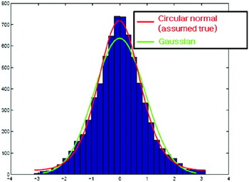
A circular normal distribution is the normal distribution for the circular random variable, which is appropriate for carrier phase observables, which are the measurements of the fractional phase (Cai and Grafarend, Reference Cai and Grafarend2007). After conducting the test of uniformity and the test of goodness of fit on circular normal distributions, Cai and Grafarend concluded that GPS carrier observables can be characterized more precisely using the circular normal distribution. Figure 1 shows the histogram of carrier observables, the Probability Density Functions (PDFs) of a Gaussian distribution and a circular normal distribution. The figure verifies that the circular normal distribution is more appropriate than the Gaussian distribution to describe a carrier phase error. In this paper, the circular normal distribution is assumed to be the true error distribution in the simulation.

Figure 1.

Statistics of carrier observables.

The PDF of the circular normal distribution is given as Equation (1).

(1)

$p\lpar \theta \semi {\kern 1pt} \mu _{\setnum{0}} \comma \kappa \rpar \equals {1 \over {2\pi I_{\setnum{0}} \lpar \kappa \rpar }}\exp \lpar \kappa \cos \lpar \theta \minus \mu _{\setnum{0}} \rpar \rpar \comma \quad \minus \pi \les \theta \les \pi \comma$

where I ₀(κ) is the modified Bessel function, μ₀ is the mean direction, and κ is the concentration parameter. These parameters can be determined from the sufficient number of carrier phase observables.

Since the carrier phase measurement error has a heavier tail distribution than a Gaussian distribution, in the conventional CRAIM algorithm that insists on Gaussian assumption, sigma-overbounding methods are used to prevent integrity risks (Shively and Braff, Reference Shively and Braff2000; Varner, Reference Varner2002; Rife et al, Reference Rife, Pullen and Pervan2004). A sigma-overbounding is a procedure used to set an inflation factor to make the user's protection level bound to the true position error in required missed detection rate. It makes the system meet the integrity requirement:

(2)

$\sigma _{over} \equals INF \cdot \sigma$

where INF is the inflation factor determined using Equation (3).

(3)

$\eqalign{\tab\hskip74pt INF \equals {M \over {5{\cdot}81}}\comma \cr \tab \int_{\rm M}^{\infty } {p_{true} \lpar x\rpar\, dx \equals } \int_{\setnum{5{\cdot}81}}^{\infty } {p_{N\lpar \setnum{0}\comma \setnum{1}\rpar } \lpar x\rpar\, dx \equals 3{\cdot}12 \times 10^{ \minus \setnum{9}} } \cr}$

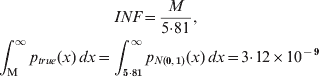
where p _true (x) is the observed true PDF. The denominator value of 5·81 is a multiplier used to calculate a defined, fault-free protection level (RTCA, 2001). This method provides users with an overbounded broadcast sigma that they can use to estimate the fault-free protection levels for bounding position errors with the required probability. Figure 2 shows PDFs of a true error model and an Overbound Gaussian (OG) distribution. As the figure shows, the overbound Gaussian model is too conservative in preventing the integrity risk (i.e. following the true tail probability), so this method has disadvantages in the accuracy aspect. Therefore, an alternative error model that is more similar to the true PDF has to be used. This paper proposes a new CRAIM algorithm using a Gaussian sum filter which can deal with non-Gaussian error distributions.

Figure 2.

PDF of true error model and overbound Gaussian distribution.

3. GAUSSIAN MIXTURE MODELLING METHOD

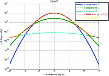
In order to implement a Gaussian sum filter, a Gaussian Mixture Model (GMM), which precisely follows a true error model, has to be generated. In Figure 3, the true error model (yellow line) is approximated by the weighted sum of the three Gaussian distributions and indicated in the red line. This red line is called the Gaussian Mixture Model. In GMM, the j-th measurement error distribution can be expressed by a sum of N _comp Gaussian distributions as follows:

(4)

${\rm p}_{GM} \lpar n^{j} \rpar \equals \sum\limits_{i \equals \setnum{1}}^{N_{\rm comp} } {\gamma ^{\lt i \gt } {\rm p}_{\rm N} \lpar n^{j} \semi{\kern 1pt}m^{j \comma\! \lt i \gt } \comma v^{j\comma\! \lt i \gt } \rpar } \comma$

where γ^ is the weight of the i-th GMM component, $\sum\limits_{i \equals \setnum{1}}^{N_{comp} } {\gamma ^{ \lt i \gt } } \equals 1$ , p _N (x, m, C) is the Gaussian probability density of x, m is mean, and C is variance.

Figure 3.

Gaussian mixture model.

The parameter p _GM converges to any density function as N _comp increases and the covariance approaches the zero matrix. In general, the parameters N _comp, γ^, m ^j,, and ν^j, are selected by the Expectation Maximization (EM) algorithm, which is a general approach to iterative computation of maximum-likelihood estimates (Dempster et al, Reference Dempster, Laird and Rubin1977; Vlassis et al, Reference Vlassis, Papaconstantinou and Tsanakas1999; Vlassis and Likas Reference Vlassis and Likas2002). However, this algorithm is not appropriate for the integrity-monitoring problem because its main concern is overall fitting of the given PDF, and it does not deal properly with the tail probability.

This paper proposes a new method for accurate fitting of the tail probability and overall probability as well. If one defines the performance index J as Equation (5) and using the optimization technique, it is possible to obtain the modelling parameters that minimize J.

(5)

$J \equals \int_{\setnum{0}}^{\infty } {e^{x} \log \left( {f\left( {e^{x} } \right)} \right)}\, dx$

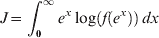
where f(x)=[p _GM(x)−p _GL(x)]². The performance index is on a logarithmic scale to emphasize the small tail probability.

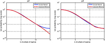
Figure 4 (Left) shows PDFs of the true error model and the Gaussian Mixture Model approximated by an EM algorithm. The EM algorithm estimates the core part very accurately and fails to deal properly with the tail part. Because the tail part has a very small probability density, the EM algorithm neglects the tail when it calculates expectation. However, the proposed algorithm sets the Gaussian mixture parameters which emphasize the tail probability, a very important aspect in integrity monitoring. As a result, as shown in Figure 4 (Right), the tail part also can be approximated accurately by using the proposed algorithm.

Figure 4.

True error model (blue) and Gaussian Mixture Model (red) for EM algorithm (Left) and the proposed algorithm (Right).

In this work, N _comp was fixed to 3 and m ^j, to 0, because the carrier phase error model is a uni-modal Gaussian-like model, and it is assumed to have a zero mean. The variables γ^and ν^j, were optimized by a Sequential Quadratic Programming (SQP) algorithm.

4. GAUSSIAN SUM FILTER

A Gaussian Mixture Model can be designed using the above method for any carrier phase error model. Assuming that the carrier phase measurement error follows the GMM, several Kalman filters that deal with each Gaussian component are used to estimate the distribution of states more accurately. This method is called the Gaussian Sum Filter (GSF) (Alspach and Sorenson, Reference Alspach and Sorenson1972; Fruhwirth, Reference Fruhwirth1997; Ito and Xiong, Reference Ito and Xiong2000).

Provided that all of the measurements are independent, a probability distribution of the measurement vector is obtained by the following equation:

(6)

$p\lpar n\rpar \equals \prod\limits_{j \equals \setnum{1}}^{N_{M} } {p_{GM} \lpar n^{j} \rpar \equals } \prod\limits_{j \equals \setnum{1}}^{N_{M} } {\left( {\sum\limits_{i \equals \setnum{1}}^{Ncomp} {\gamma ^{ \lt i \gt } p_{N} \left( {n^{j} \semi {\kern 1pt} m^{j\comma \lt i \gt } \comma \nu ^{j\comma \lt i \gt } } \right)} } \right)}$

where N _M is the number of measurements. Equation (6) can be expressed by a weighted sum of multivariate normal distributions as:

(7)

$p\lpar n_{k} \rpar \equals \sum\limits_{i \equals \setnum{1}}^{N_{\rm {mode}} } {\varpi _{k} ^{\hskip4pt \lt i \gt } p_{N} \left( {n_{k} \semi {\kern 1pt} M_{k} ^{ \hskip4pt\lt i \gt } \comma R_{k} ^{\hskip4pt \lt i \gt } } \right)} \comma$

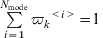where N _mode is the number of modes, $N_{\rm {mode}} \equals \lpar N_{comp} \rpar ^{N_{M}}$ , and ϖ_k^ is a weight of the i^th multivariate Gaussian distribution. ϖ_k^ is calculated from Equation (6) and $\sum\limits_{i \equals \setnum{1}}^{N_{\rm {mode}} } {\varpi _{k}^{\hskip4pt\lt {i}\gt } } \equals 1$ .

In this work, the system is linear, and the mean of measurement error was assumed to be zero. In this case, GSF can be formulated by implementing the Kalman filters for every Gaussian component as follows: First, by propagating the past state and covariance of each Gaussian component, the current state and covariance can be calculated as Equations (8) and (9). Using these values, a priori probability distribution of state can be expressed as Equation (10).

(8)

$\tilde{x}_{k} ^{\hskip3pt \lt j \gt } \equals F_{K} \hat{x}_{k \minus \setnum{1}} ^{\hskip14pt \lt j \gt } \comma$

(9)

$\tilde{P}_{k} ^{\hskip3pt \lt j \gt } \equals F_{K} \tilde{P}_{k \minus \setnum{1}} ^{\hskip12pt \lt j \gt } F_{K} ^{\hskip5pt T} \plus Q_{k \minus \setnum{1}} \comma$

(10)

$p\left( {x_{k} \left\vert {z_{\setnum{1}\colon k \minus \setnum{1}} } \right.} \right) \equals \sum\limits_{j \equals \setnum{1}}^{N_{{post}} } {\pi _{k}^{ \hskip4pt\lt j \gt } p_{N} \left( {x_{k} \semi {\kern 1pt} \tilde{x}_{k}^{ \hskip4pt\lt j \gt } \comma \tilde{P}_{k}^{ \hskip4pt\lt j \gt } } \right)} \comma$

where $\tilde{x}_{k}$ is the time propagated state vector at time index k, $\hat{x}_{k}$ is the measurement updated state vector at time index k, z _1:k is the measurement set up to time index k, F _K is a system mode applied to the previous state, P is the estimation error covariance matrix, Q is the process noise covariance matrix, and π_k^<j> is a weight of the j^th priori probability distribution, $\sum\limits_{j \equals \setnum{1}}^{N_{{post}} } {\pi _{k}^{\hskip3pt \lt j \gt }\equals 1.}$

From Equation (7), the likelihood function of the current epoch is expressed as:

(11)

$p\left( {z_{k} \vert x_{k} } \right) \equals \sum\limits_{i \equals \setnum{1}}^{N_{{{\rm mode}}} } {\varpi _{k} ^{\hskip4pt \lt i \gt } p_{N} \left( {z_{k} \semi {\kern 1pt} H_{k} x_{k} \comma R_{k} ^{ \hskip4pt\lt i \gt } } \right)} \comma$

where H _k is the observation matrix, and R _k is the observation noise covariance matrix.

GSF updates the weights of the Gaussian components, the states, and the covariance matrix by using Equations (12)–(14).

(12)

$\omega _{k} ^{\hskip4pt \lt i\comma j \gt } \propto \varpi _{k} ^{ \hskip4pt\lt i \gt } \pi _{k} ^{ \hskip4pt\lt j \gt } p\left( {z_{k} \semi {\kern 1pt} H_{k} \tilde{x}_{k} ^{\hskip4pt \lt j \gt } \comma R_{k} ^{ \hskip4pt\lt i \gt } \plus H_{k} \tilde{P}_{k} ^{ \hskip4pt\lt j \gt } H_{k} ^{\hskip3ptT} } \right)\comma$

where $\sum\limits_{i \equals \setnum{1}}^{N_{\rm {mode}}} {\sum\limits_{j \equals \setnum{1}}^{N_{\rm {post}} } {\omega _{k} ^{\hskip3pt \lt i\comma j \gt } \equals 1}. }$

(13)

$\hat{x}_{k} ^{ \hskip3pt\lt i\comma j \gt } \equals \tilde{x}_{k} ^{\hskip3pt \lt j \gt } \plus \hat{P}_{k} ^{\hskip3pt \lt i\comma j \gt } H_{k} ^{\hskip3pt T} \left( {R_{k} ^{\hskip3pt \lt i \gt } } \right)^{ \minus \setnum{1}} \left( {z_{k} \minus H_{k} \tilde{x}_{k} ^{\hskip3pt \lt j \gt } } \right)$

(14)

$\hat{P}_{k} ^{\hskip3pt \lt i\comma j \gt } \equals \left[ {\left( {\tilde{P}_{k} ^{ \hskip3pt\lt j \gt } } \right)^{\! \minus \setnum{1}} \plus H_{k} \left( {R_{k} ^{ \hskip3pt\lt i \gt } } \right)^{\! \minus \setnum{1}} H_{k} ^{\hskip3pt T} } \right]^{ \minus \setnum{1}}$

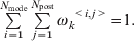
Using these updated weights, states, and covariance, the current states are estimated as follows:

(15)

$p\left( {x_{k} \vert z_{\setnum{1}\colon k} } \right) \equals \sum\limits_{i \equals \setnum{1}}^{N_{{{\rm mode}}} } {\sum\limits_{j \equals \setnum{1}}^{N_{{{\rm post}}} } {\omega _{k} ^{ \hskip3pt\lt i\comma j \gt } p_{N} \left( {x_{k} \semi {\kern 1pt}\hat{x}_{k} ^{ \hskip3pt\lt i\comma j \gt } \comma \hat{P}_{k} ^{ \hskip3pt\lt i\comma j \gt } } \right)} }$

5. INTEGRITY MONITORING ALGORITHMS

GNSS-based navigation systems must have an integrity-monitoring system that contains two main functions: 1) detection and exclusion of satellite faults and 2) estimation of the uncertainty of the position solutions. First, the system calculates decision variables and compares these to thresholds that have been set to satisfy the integrity requirements for the desired operation. If any decision variable exceeds the threshold, the system concludes that the corresponding measurement contains a fault and excludes the detected fault. Second, because the system cannot distinguish the true position estimation errors, it estimates the uncertainty of the solution, which is known as the protection level.

5.1. Fault Detection and Exclusion

The proposed algorithm uses an individual residual method for fault detection and exclusion (FDE). The conventional χ² FDE method presumes that the residuals follow the Gaussian distribution, and thus it cannot be implemented in a non-Gaussian model. Furthermore, it is very hard for a conventional χ² FDE to distinguish small faults because it detects the fault in a system by inspecting a decision variable calculated from Weighted Squared Sum of the Errors (WSSE) that follows a χ² distribution, not individual errors. On the contrary, as the individual residual method detects the fault by examining each residual, not the combined one, it can distinguish smaller faults than conventional FDE methods can.

In the KFIR method, the algorithm compares a measurement residual with the multiple of the residual standard deviation. Because GSFIR, assumes a non-Gaussian error, it cannot use the residual standard deviation. Instead, GSFIR estimates the residual distribution, and then decides whether the residual is located in a normal region or not. These individual residual algorithms have to estimate the residual distribution and determine the individual detection threshold for each residual. The expected measurement is obtained by projecting the propagated state from the position domain to the measurement domain, and the residual is defined as the difference between the true and expected measurements. For a Gaussian sum filter, the residual of the j-th measurement's i-th Gaussian component can be calculated as:

(16)

$r_{k} ^{ \hskip3pt\lt i\comma j \gt } \equals H_{k} \tilde{x}_{k} ^{ \hskip3pt\lt i \gt } \minus z_{k} ^{\hskip3pt \lt j \gt } \comma$

The associated weights and the covariance are as follows:

(17)

$\omega _{k} ^{ \hskip3pt\lt i\comma j \gt } \equals \omega _{k} ^{ \hskip3pt\lt i \gt } \varpi _{k} ^{ \hskip3pt\lt j \gt } \comma$

(18)

$C_{r\comma k}^{ \hskip8pt\lt i\comma j \gt } \equals H_{k} \tilde{P}_{k} ^{ \hskip3pt\lt i \gt } H_{k}^{T} \plus R_{k}^{ \hskip3pt\lt j \gt }.$

Therefore, the residual distribution from the Gaussian sum filter is expressed as:

(19)

$p_{R_{k} } \lpar r_{k} \rpar \equals \sum\limits_{l \equals \setnum{1}}^{N_{{post}} } {\omega _{k} ^{ \hskip3pt\lt l \gt } p_{N} \left( {r_{k} \semi {\kern 1pt} r_{k} ^{ \hskip3pt\lt l \gt } \comma C_{r\comma k} ^{ \hskip8pt\lt l \gt } } \right)}$

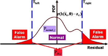
As shown in Figure 5, the expectation of the residual is close to zero and the large residuals have low probabilities. When the expectation of the residual is in the region between the two thresholds known as the normal region, the system declares that there is no fault in the measurement. Otherwise, it determines that the measurement includes a fault, and excludes it for further operation.

Figure 5.

PDF of a residual distribution and thresholds.

In real implementation, a one-sided tail probability can be calculated below or above zero depending on the decision variable shown in Equation (20). The result of this calculation is compared with the individual false alarm rate that will be defined in the next subsection for each measurement.

(20)

$pr_{k} ^{\hskip6pt j} \equals \left\{\openup3 {\matrix{ {\int_{\! \minus \infty }^{\setnum{0}} {p_{R_{k} ^{\hskip3pt j} } \left( {r_{k} ^{\hskip4pt j} \prime} \right)\,dr_{k} ^{\hskip4pt j} \prime} \comma r_{k} ^{\hskip4pt j} \ges 0} \cr {\int_{\setnum{0}}^{\infty } {p_{R_{k} ^{\hskip4pt j} } \left( {r_{k} ^{\hskip4ptj} \prime} \right)\,dr_{k} ^{\hskip4pt j} \prime} \comma r_{k} ^{\hskip4pt j} \lt 0} \cr} } \right..$

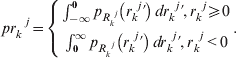
The individual residual method requires a threshold for each measurement, and hence the individual false alarm rate, p _fa, needs to be determined first. In this paper, the multivariate normal distribution is used, and the residual covariance matrix is estimated from the Kalman filter. Therefore, assuming that the individual false alarm rates for all residuals are the same, the following equation is obtained:

(21)

$P_{FA} \equals 2\left( {1 \minus {1 \over {\sqrt {\vert C_{r} \vert \lpar 2\pi \rpar ^{N_{M} } } }}\int\limits_{ \minus \infty }^{K\sigma _{\setnum{1}} } {\int\limits_{ \minus \infty }^{K\sigma _{\setnum{2}} } { \ldots \int\limits_{ \minus \infty }^{K\sigma _{{N_{M} }} } {\exp \left( { \minus {1 \over 2}r^{T} C_{r} r} \right)dr} } } }\hskip2pt \right)\comma$

where P _FA is the predefined false alarm rate, and σ_i is the i-th diagonal term of C _r. K is the only unknown in this equation, and it can be solved by iteration. With the K determined, the individual false alarm rate is calculated as follows:

(22)

$P_{fa\comma i} \equals 2\int_{K\sigma _{i} }^{\infty } {p_{R_{i} }\ \lpar r_{i} \rpar \,dr_{i} } \equals 2\int_{K}^{\infty } {p_{N\lpar \setnum{0}\comma \setnum{1}\rpar } \lpar n\rpar\, dn} \equals P_{fa}$

Because it is assumed that the measurement error follows a symmetrical distribution, the proposed algorithms declare that a fault is present if a one-sided tail probability of a residual pr _k^j exceeds the value of ${{P_{fa}} \big/ 2}$ .

5.2. Protection Level

Navigation users must calculate both fault-free and faulted protection levels for integrity. The faulted protection levels indicate the position error protection, assuming that a fault measurement exists. Assuming the measurement errors are Gaussian (SSX2, KFX2, KFIR), the protection levels can be calculated from the standard deviation of measurements, computing parameters such as k _md, k _ffmd and a detection threshold (RTCA, 2001). The parameters for computing protection levels are shown in Table 1.

Table 1.

Multipliers for protection level calculation.

In GSFIR it is assumed that the measurement errors are non-Gaussian and the protection levels have to be calculated in a different way. Using Equations (23)–(26)HPL _0,n, VPL _0,n, HPL _1,n and VPL _1,n can all be calculated. The subscripts 0 and 1 denote ‘fault free’ and ‘faulted’, respectively, and the subscript n is the protection level component due to noise.

(23)

$\int_{ \minus \infty }^{k_{{md}} } {p_{N} \,\left( {n\semi {\kern 1pt}0\comma 1} \right)\,dn \equals \int_{ \minus \infty }^{ePL_{{\setnum{1}\comma n}} } {p_{\hat{x}_{k}\ \lpar \setnum{1}\rpar } } } \lpar x_{\setnum{1}} \rpar\, dx_{\setnum{1}} \comma$

(24)

$\int_{ \minus \infty }^{k_{{md}} } {p_{N} \,\left( {n\semi {\kern 1pt}0\comma 1} \right)\,dn \equals \int_{ \minus \infty }^{nPL_{{\setnum{1}\comma n}} } {p_{\hat{x}_{k}\ \lpar \setnum{2}\rpar } } } \lpar x_{\setnum{2}} \rpar\, dx_{\setnum{2}} \comma$

(25)

$HPL_{\setnum{1}\comma n} \equals \sqrt {ePL_{\setnum{1}\comma n} ^{\hskip10pt\setnum{2}} \plus nPL_{\setnum{1}\comma n} ^{\hskip10pt\setnum{2}} } \comma$

(26)

$\int_{ \minus \infty }^{k_{{md}} } {p_{N} \,\left( {n\semi {\kern 1pt} 0\comma 1} \right) \equals \int_{ \minus \infty }^{VPL_{{\setnum{1}\comma n}} } {p_{\hat{x}_{k}\ \lpar \setnum{3}\rpar } } } \lpar x_{\setnum{3}} \rpar\, dx_{\setnum{3}}.$

XPL _0,n can be calculated when k _md is replaced by k _ffmd in Equations (23)–(26).

Using XPL _0,n, XPL _1,n and Equations (27)–(31), the XPL with non-Gaussian measurement errors can be calculated.

(27)

$HPL_{\setnum{0}} \equals HPL_{\setnum{0}\comma n} \comma$

(28)

$VPL_{\setnum{0}} \equals VPL_{\setnum{0}\comma n} \comma$

(29)

$HPL_{\setnum{1}}^{j} \equals HPL_{\setnum{1}\comma n} \plus \left\vert {T^{\hskip2pt j} \sqrt {H_{W}^{ \plus } \, \left( {1\comma j} \right)^{\setnum{2}} \plus H_{W}^{ \plus } \,\left( {1\comma j} \right)^{\setnum{2}} } } \right\vert \equals HPL_{\setnum{1}\comma n} \plus HPL_{b}^{j}$

(30)

$VPL_{\setnum{1}}^{j} \equals VPL_{\setnum{1}\comma n} \plus \left\vert {T^{\hskip 2ptj} \cdot H_{W}^{ \plus } \,\lpar 3\comma j\rpar } \right\vert \equals VPL_{\setnum{1}\comma n} \plus VPL_{b}^{j} \comma$

(31)

$H_{W}^{ \plus } \equals \left( {H^{T} WH} \right)^{ \minus \setnum{1}} WH^{T} \comma$

where W is a weighting matrix, the subscript ‘1’ indicates the faulted protection level under the assumption that the measurement has a fault, the subscript b is the protection level component due to bias, and T ^j is calculated from the probability distribution of the residual and individual false alarm rates as:

(32)

$p_{fa} \equals 2\int_{T^{j} }^{\infty } {p_{R_{k}^{j} } \lpar r_{k}^{j} \rpar \,dr_{k}^{j} }$

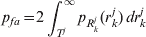
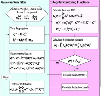
Figure 6 shows the overall flowchart of the proposed algorithm. The Gaussian sum filter estimates the state probability distribution from which the residual distribution is estimated. With these distributions, the integrity monitoring function performs fault detection or exclusion and protection level calculations.

Figure 6.

Flowchart of integrity monitoring algorithm using a Gaussian sum filter.

6. SIMULATION

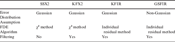
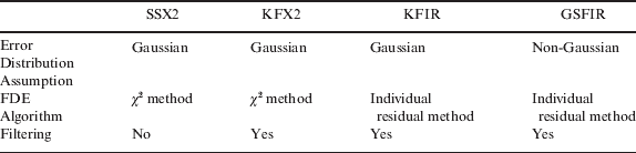
A simulation was performed to validate the proposed CRAIM algorithm based on a Gaussian sum filter. In order to investigate the advantage of the non-Gaussian assumption, conventional methods were implemented in parallel. These methods are summarized in Table 2.

Table 2.

Four methods implemented in simulation.

6.1. Simulation Setup

The system model and the measurement equation were defined using the linear functions in Equations (33) and (34). The linear functions are used because the validation focused on the effect of the non-Gaussian error distribution and not the nonlinearity. The user position in ENU coordinates and the receiver clock bias were defined as state variables. The user was assumed to be static and a 24 GPS satellite constellation was generated for 100 epochs.

(33)

$x_{k} \equals f_{k} \hskip2pt\left( {x_{k \minus \setnum{1}} \comma v_{k \minus \setnum{1}} } \right) \equals Fx_{k \minus \setnum{1}} \plus v_{k \minus \setnum{1}} \comma$

(34)

$z_{k} \equals h_{k} \,\left( {x_{k} \comma n_{k} } \right) \equals H_{k} x_{k} \plus n_{k} \comma$

where $z_{k} \equals \left( {e_{u}^{\setnum{1}} \cdot R^{\setnum{1}} \minus \rho _{u}^{\setnum{1}} \comma e_{u}^{\setnum{2}} \cdot R^{\setnum{2}} \minus \rho _{u}^{\setnum{2}} \comma \cdots \comma e_{u}^{n_{M} } \cdot R^{n_{M} } \minus \rho _{u}^{n_{M} } } \right)_{k} ^{T}$ , $x_{k} \equals \left[ {x_{e} \ x_{n} \ x_{u} \ x_{t} } \right]^{T}$ , $H_{k} \equals \left( {\matrix{ {e_{u}^{\setnum{1}} } \tab {e_{u}^{\setnum{2}} } \tab \cdots \tab {e_{u}^{n_{M} } } \cr { \minus 1} \tab { \minus 1} \tab \cdots \tab { \minus 1} \cr} } \right)_{k} ^{T}$ , 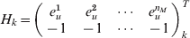and F=I _4×4.

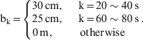
The measurement error is generated using the assumed distribution shown in Equation (1). The simulator intentionally injected biases into the pseudorange of a satellite as follows:

${\rm {b}}_{\rm {k}} \equals \left\{\! {\matrix{{{ 30\,{\rm cm}\comma \ }} \tab {{\rm k} \equals 20 \sim 40\,{\rm s}} \cr {{25\, {\rm cm}\comma \ }} \tab {{\rm k} \equals 60 \sim 80\,{\rm s}} \cr { \hskip-12pt0\,{\rm m}\comma }\tab {\hskip-12pt{\rm otherwise}} \cr} } \right..$

The four algorithms listed in Table 2 were used to detect and exclude the fault and to estimate the protection levels.

6.2. Simulation Results

The simulation results were classified into measurement domain results, position domain results, and processing time for each algorithm.

6.2.1. Measurement Domain Results

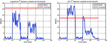
Figure 7 shows the decision variables (WSSE) and the thresholds of the SSX2 and the KFX2 algorithms. When a decision variable exceeded the threshold, the system declared a fault. The SSX2 method could not detect any faults because the noise level was too high. The KFX2 method detected the 25 cm bias initially, but it failed to detect any bias thereafter. When a filtering method fails to detect and exclude a bias, the remaining bias propagates through the filter so that subsequent detection becomes more difficult.

Figure 7.

Decision variable and threshold of SSX2 (Left) and KFX2 (Right).

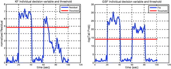
Figure 8 shows the decision variables and the thresholds of the KFIR and the GSFIR algorithms. The KFIR method detected the 30 cm bias perfectly, but it did not detect a 25 cm bias after 67 s. The undetected bias remained in the filtering process and led to a large position error that propagated into subsequent processes. The error eventually resulted in the monitoring system becoming noisy after the missed detection. The GSFIR methods detected the faults at all epochs where the system had a fault measurement.

Figure 8.

Decision variable and threshold of KFIR (Left) and GSFIR (Right).

In this simulation, the minimum detectable bias was about 25·0 cm for the KFIR method and about 20·4 cm for the GSFIR method. Therefore, the simulation proved that GSFIR can detect a smaller bias than the other conventional methods.

6.2.2. Position Domain Results

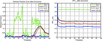
Figure 9 shows the vertical position errors and the vertical protection levels for each algorithm after the FDE procedure. Since the SSX2, KFX2, and KFIR methods did not detect the faults well, they exhibited large position errors induced by the remaining faults. However, the GSFIR detected and excluded all 30 cm and 25 cm biases perfectly and provided the most accurate position solutions. The values of position errors and protection levels of each method are shown in Table 3. The SSX2 method has the highest protection levels because it has the highest level of noise, and the KFX2 method provided a slightly higher protection level than KFIR, which means that the KFIR method could detect smaller biases. The protection levels of the GSFIR method were the lowest, and this indicates that the proposed algorithm outperformed the other algorithms in terms of integrity and availability. Once the detected fault measurement is excluded, the protection levels increase in the faulty period because a smaller number of measurements are available.

Figure 9.

Vertical position errors (Left) and vertical protection levels (Right) of each method.

Table 3.

Position errors and protection levels of each method.

6.2.3. Processing Time

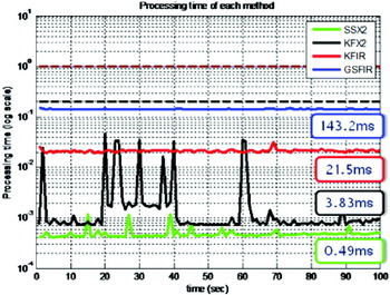
Figure 10 shows the processing time of each algorithm. In the figure, the two dashed lines are the maximum allowable processing times for real time implementation.

Figure 10.

Processing time of each algorithm.

The computational inefficiency of the non-Gaussian filter is the main acknowledged criticism. However, the simulation results show that the proposed algorithm can be implemented in real time up to 5 Hz. Because the carrier phase error distribution is almost Gaussian, a Gaussian sum filter can be implemented with a small number of Gaussian components.

6.3. Discussion of the Results

The simulation results and their analysis can be summarized as follows:

• The result of the SSX2 method was the worst due to the high noise level. KFX2 and KFIR use the same filtering method with different decision variables (WSSE and individual residual, respectively). For the same false alarm rate, the WSSE method has a larger detection threshold than the individual residual method has because it needs to consider the noise of the other fault-free measurement. Therefore, the individual residual method that considers only one measurement at a time has a lower threshold, better fault detection performance, and better availability.
• GSFIR and KFIR use the same FDE algorithm, but use different error model and filtering methods. GSFIR used the non-Gaussian error model, while KFIR used the overbound Gaussian error model. The overbound Gaussian model estimates the error distribution conservatively to prevent the integrity risk while keeping the Gaussian assumption, and thus it has a higher protection level and detection threshold.
• Although the major acknowledged criticism of the Gaussian sum filter is its computational inefficiency, it can be implemented in real time in ordinary PCs. There is no need to have many GMM components because carrier phase error distribution is almost Gaussian.

These results validated the proposed algorithm in terms of fault detection and exclusion availability.

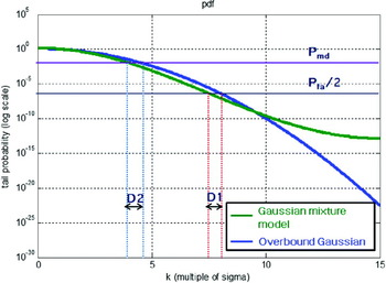
The results can be explained with Figure 11, which shows the tail probability of a residual from the Kalman filter and the Gaussian sum filter. The Kalman filter used the overbound Gaussian to meet the integrity requirements and the Gaussian sum filter used the Gaussian mixture model that precisely follows the true error model. The detection threshold and the protection levels are determined using the residual distribution, false alarm rate, and missed detection rate. The difference of the error models results in the gap of the residuals at the given probabilities. The gaps, D1 and D2, cause higher detection thresholds and protection levels for the conventional CRAIM method.

(35)

$\left. T \right\vert_{KFIR} \equals \left. T \right\vert_{GSFIR} \plus {\rm D1}$

(36)

$\left. {{\rm VPL}_{n} } \right\vert_{KFIR} \equals \left. {{\rm VPL}_{n} } \right\vert_{GSFIR} \plus \sum\limits_{i \equals \setnum{1}}^{N_{M} } {{\bf H}_{W}^{ \plus } \lpar 3\comma i\rpar \cdot {\rm D2}\lpar i\rpar }$

Figure 11.

The effect of overbound sigma.

7. CONCLUSIONS

In this paper, a CRAIM algorithm, which tests individual measurement residuals using a Gaussian sum filter, was developed. To represent a non-Gaussian carrier phase error model, a Gaussian mixture modelling method using the optimization technique, was introduced. The simulation results showed that the proposed algorithm could detect smaller measurement bias and generate smaller protection levels than other conventional methods. This result implied that the proposed algorithm could provide better integrity monitoring performance than other conventional methods that assume a measurement model to be Gaussian. The conservative sigma overbounding methods deteriorated the integrity monitoring performance. Using a more accurate error model, a navigation system can provide higher availability without integrity losses.

Although the proposed algorithm requires high computational capacity, the simulation results showed that a real-time process was possible to implement in an ordinary PC. Therefore it could be used in many sophisticated systems, such as reference stations, monitor stations, and airliners, or for development and performance assessment of sigma overbounding methods in conventional systems. In the future, more computationally efficient algorithms need to be developed for the proposed method to be widely used.

ACKNOWLEDGMENT

This research was supported in part by the Institute of Advanced Machinery and Design, Institute of Advanced Aerospace Technology at Seoul National University, the Ministry of Land, Transport and Maritime Affairs, Agency for Defense Development and the Brain Korea 21 (BK-21) program.

References

REFERENCES

[1]Lee, Y. C. (1986) “Analysis of range and position comparison methods as a means to provide GPS integrity in the user receiver,” presented at the ION 42^nd Annual Meeting, Seattle, WA.Google Scholar

[2]Parkinson, B. W. and Axelrad, P. (1988) “Autonomous GPS integrity monitoring using the pseudorange residual.” The Journal of Navigation, 35, 255–274.CrossRef Google Scholar

[3]Kim, D. and Langley, R., “GPS ambiguity resolution and validation: Methodologies, trends and issues,” presented at the 7^th GNSS Workshop – International Symposium on GPS/GNSS, Seoul, Korea, Nov. 2000.Google Scholar

[4]Rife, J., Khanafseh, S., Pullen, S., Lorenzo, D., Kim, U., Koenig, M., Chiou, T., Kempny, B. and Pervan, B., “Navigation, interface suppression, and fault monitoring in the sea-based joint precision approach and landing system,” Proceedings of the IEEE, Vol. 96, No. 12, pp. 23–53, 2008.CrossRef Google Scholar

[5]Pervan, B. S., Lawrence, D. G. and Parkinson, B. W., “Autonomous fault detection and removal using GPS carrier phase,” IEEE Transactions on Aerospace and Electronic Systems, 34, 3, pp. 897–906, 1998.CrossRef Google Scholar

[6]Feng, S., Ochieng, W., Moore, T., Hill, C., and Hide, C., “Carrier phsed-based integrity monitoring for high-accuracy positioning,” GPS Solutions, 13, 1, pp. 13–22, 2007.CrossRef Google Scholar

[7]Alspach, D. L. and Sorenson, H. W., “Nonlinear Bayesian estimation using Gaussian sum approximations,” IEE Transactions on Automatic Control, AC-17, 4, pp. 439–477, 1972.CrossRef Google Scholar

[8]Fruhwirth, R., “Track fitting with non-Gaussian noise,” Computer Physics Communications, 100, 1–16, 1997.CrossRef Google Scholar

[9]Ito, K. and Xiong, K., “Gaussian filters for nonlinear filtering problems,” IEEE Transactions on Automatic Control, 45, pp. 910–927, 2000.CrossRef Google Scholar

[10]Da, R. and Lin, C., “A new failure detection approach and its applications to GPS autonomous integrity monitoring,” IEEE Transactions on Aerospace and Electronics Systems, 30, pp. 499–506, 1995.Google Scholar

[11]McGraw, G. A., Murphy, T., Brenner, M., Pullen, S. and Van, A. J., “Development of the LAAS accuracy models,” presented at the ION GPS 2000, pp. 1212–1223. 2000.Google Scholar

[12]Sayim, I., Pervan, B., Pullen, S. and Enge, P., “Experimental and theoretical results on the LAAS sigma overbound,” presented at the ION GPS 2002.Google Scholar

[13]Cai, J. and Grafarend, E. W., “The statistical property of the GNSS carrier phase observations and its effects on the hypothesis testing of the related estimators,” presented at the ION GNSS 2007, 24–28, Sep., Fort worth, Texas, 2007.Google Scholar

[14]Shively, C. A. and Braff, R., “An overbound concept for psedorange error from the LAAS ground facility,” MP00W0000138, The MITRE Corporation.Google Scholar

[15]Varner, C., “Gaussian and mixed Gaussian methods of LAAS overbounding,” presented at the ION National Technical Meeting 2002, San Diego, CA., January, 2002.Google Scholar

[16]Rife, J., Pullen, S. and Pervan, B., “Core overbounding and its implications for LAAS integrity,” presented at the ION GNSS2004.Google Scholar

[17]RTCA Special Committee 159 Working Group 2, “Minimum operational performance standards for global positioning system/ wide area augmentation system airborne equipment,” RTCA Document Number DO-229C, 2001.Google Scholar

[18]Dempster, A. P., Laird, N. M. and Rubin, D. B., “Maximum likeligood from incomplete data via the EM algorithm,” Journal of the Royal Statictical Society, Series B, Vol. 39, No. 1, pp. 1–38, 1977.Google Scholar

[19]Vlassis, N. A., Papaconstantinou, G. and Tsanakas, P.,. “Mixture density estimation based on maximum likelihood and sequential test statistics,” Neural processing letters, 9, pp. 63–76, 1999.CrossRef Google Scholar

[20]Vlassis, N. A. and Likas, A., “A greedy EM algorithm for Gaussian mixture learnin,” Neural processing letters, 15, pp. 77–87, 2002.CrossRef Google Scholar