1 Introduction
The flow-induced instability and flapping dynamics of a flexible flag have been the subject of many previous experimental, numerical and analytical studies (Theodorsen & Mutchler Reference Theodorsen and Mutchler1935; Kornecki, Dowell & O’Brien Reference Kornecki, Dowell and O’Brien1976; Huang Reference Huang1995; Zhang et al. Reference Zhang, Childress, Libchaber and Shelley2000; Zhu et al. Reference Zhu, Wolfgang, Yue and Triantafyllou2002; Shelley, Vandenberghe & Zhang Reference Shelley, Vandenberghe and Zhang2005; Connell & Yue Reference Connell and Yue2007; Eloy, Souilliez & Schouveiler Reference Eloy, Souilliez and Schouveiler2007). This configuration can be considered as a simple example of a broader class of fluid–structure interaction problems which deal with the interaction between flexible bodies and flows. This simple system also contains physical processes that form the foundation of many applications such as human snoring (Tetlow & Lucey Reference Tetlow and Lucey2009), wing fluttering (Tang, Yamamoto & Dowell Reference Tang, Yamamoto and Dowell2003), fish and insect propulsion mechanisms (Lighthill Reference Lighthill1975; Michelin & Smith Reference Michelin and Smith2009; Shoele & Zhu Reference Shoele and Zhu2012, Reference Shoele and Zhu2013, Reference Shoele and Zhu2015), cooling systems (Shoele & Mittal Reference Shoele and Mittal2014) and energy harvesting systems (Miller Reference Miller1960; Kim & Davis Reference Kim and Davis1995; Guo & Paidoussis Reference Guo and Paidoussis2000).
There is significant interest and ongoing research effort in using flow-induced vibration of elastic plates to harvest energy from flow fluids (Akaydin, Elvin & Andreopoulos Reference Akaydin, Elvin and Andreopoulos2010; Wang & Ko Reference Wang and Ko2010; Doare & Michelin Reference Doare and Michelin2011; Akcabay & Young Reference Akcabay and Young2012a ,Reference Akcabay and Young b ; Cha, Kim & Porfiri Reference Cha, Kim and Porfiri2013; Michelin & Doare Reference Michelin and Doare2013; Yang, Zhao & Tang Reference Yang, Zhao and Tang2013; Zhao, Tang & Yang Reference Zhao, Tang and Yang2013). In particular, when an elastic flexible plate is placed in an axial flow, and the flow speed is higher than some critical velocity, the plate undergoes a transition from a stationary equilibrium state to a self-sustained large-amplitude flutter, which may be periodic or chaotic (Connell & Yue Reference Connell and Yue2007; Alben & Shelley Reference Alben and Shelley2008; Tang, Paidoussis & Jiang Reference Tang, Paidoussis and Jiang2009). The time-varying deflection and strain in the plate associated with the self-sustained oscillation can be used for production of electric power using deflection-based energy conversion mechanisms such as piezoelectric materials.
The conversion of beam deflection to electrical energy using piezoelectric materials has been studied previously (Sodano, Inman & Park Reference Sodano, Inman and Park2004; Anton & Sodano Reference Anton and Sodano2007; Kim, Kim & Kim Reference Kim, Kim and Kim2011). By controlling the conditions and the piezoelectric properties of the plate, it is possible to actuate the plate in its most energetic mode shape and maximize energy harvesting. However, to achieve good performance with such systems, high flow velocity is necessary and, in general, the flag must be fabricated very precisely. In fact, the dominant vibrational mode shapes of the flag need to be carefully tuned in order to coincide with its most energetic fluttering instability mode, and consequently one needs to carefully adjust the inertia and bending stiffness properties of the flag. To circumvent these difficulties, it has been suggested that placement of a bluff body such as a cylinder upstream of the plate can be a good solution since this configuration can produce vortical structures in the incident flow and promote large oscillation in a downstream piezoelectric structure without requiring careful adjustment of the structural properties of the plate (Akaydin et al. Reference Akaydin, Elvin and Andreopoulos2010). However, placement of a bluff body upstream of the plate increases system complexity, and also reduces the amount of the fluid kinetic energy available for harvesting.
In a departure from these previous studies, Kim et al. (Reference Kim, Cossé, Cerdeira and Gharib2013) examined the flow dynamics of an inverted flag (i.e. a flexible plate with a free leading edge and a fixed trailing edge) using experiments and showed that this system could sustain large-amplitude oscillations within a range of bending stiffness. They also argued that, since the system is more unstable than the conventional arrangement of a plate with a fixed leading edge, it could be a better candidate for harvesting energy from the flow. It is noted that, even though the experiments of Kim et al. (Reference Kim, Cossé, Cerdeira and Gharib2013) were for a low-aspect-ratio flag, they were designed to generate nominally two-dimensional (2D) deflection modes. This work of Kim et al. (Reference Kim, Cossé, Cerdeira and Gharib2013) has been recently followed by a 2D numerical study of dynamics of an elastic inverted flag by Ryu et al. (Reference Ryu, Park, Kim and Sung2015), which showed that 2D simulation are able to capture some key features of the flag instability as observed in the experiments. A recent three-dimensional (3D) computational study of the dynamics of an elastic inverted flag (Tang, Liu & Lu Reference Tang, Liu and Lu2015) also shows that, for an aspect ratio of the flag greater than two (aspect ratio of the flag defined as the ratio of span to chord), the results from 2D and 3D simulations are very similar and the effects of Reynolds number can be considered to be secondary.
In all the above studies (Kim et al. Reference Kim, Cossé, Cerdeira and Gharib2013; Ryu et al. Reference Ryu, Park, Kim and Sung2015; Tang et al. Reference Tang, Liu and Lu2015), the flag is assumed to be elastic and coupled to the flow, but the coupling with the piezoelectric mechanism is not considered. This has two implications: first, the effect of piezoelectric energy harvesting on the dynamics of the flag is not accounted for; and second, these studies are not able to directly analyse and quantify the energy harvesting performance. In the current paper, we expand upon these previous studies by developing and employing a fully coupled 2D fluid–structure–piezoelectric model to study both the fluid dynamics as well as energy harvesting performance of a model inverted flag. Three-dimensional effects might be important, especially for low-aspect-ratio inverted flags; but given the tremendous computational expense of 3D coupled fluid–structure–electrical simulations, as well as the associated enlargement of the parameter space in going to 3D configurations, a necessary precursor are 2D models that allow us to explore a larger parameter space and provide a baseline for interpreting the results of the 3D simulations in the future.
We begin by presenting the mathematical and numerical formulation of the 2D computational model developed for this study. This is followed by a comprehensive study of the effects of bending stiffness, flag inertia and flow Reynolds number on the dynamics of the flag, as well as their correlation with the vortex topology of the wake. In conducting this parameter survey, over 700 total 2D simulations are carried out. Finally, we focus on understanding the effect of piezoelectric parameters on the energy harvesting performance and explore scaling laws for predicting this performance.
2 Problem formulation and numerical approach
2.1 Configuration
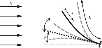
As shown in figure 1, we investigate flow-induced vibration of an inverted piezoelectric flag with length
 $L$
, placed in a uniform steady flow with velocity
 $U$
and density
 ${\it\rho}$
, with the initial inclination angle to the flow of
 ${\it\psi}$
. The flag is assumed to be inextensible, free at its leading edge and clamped at the trailing edge. It is mathematically represented as a nonlinear 2D Euler–Bernoulli beam and the position of its midline is denoted with
 $\boldsymbol{X}(s,t)$
, where
 $t$
is the time and
 $s$
is the Lagrangian coordinate along the beam, starting from
 $s=0$
at the leading edge and ending at
 $s=L$
at the trailing edge.
Schematic configuration of the inverted flag in uniform flow.

2.2 Governing equations for flow–structure interaction
The flow is governed by the incompressible Navier–Stokes equations, which in non-dimensional form are expressed as
 $$\begin{eqnarray}\displaystyle & \displaystyle \left[\frac{\partial \boldsymbol{u}}{\partial t}+\boldsymbol{{\rm\nabla}}\boldsymbol{\cdot }(\boldsymbol{u}\boldsymbol{u})\right]=-\boldsymbol{{\rm\nabla}}p+\frac{1}{Re}{\rm\nabla}^{2}\boldsymbol{u}+\boldsymbol{f}, & \displaystyle\end{eqnarray}$$
 $$\begin{eqnarray}\displaystyle & \displaystyle \boldsymbol{{\rm\nabla}}\boldsymbol{\cdot }\boldsymbol{u}=0, & \displaystyle\end{eqnarray}$$
 $({\it\rho})$
, the length of the flag
 $(L)$
and the free-stream velocity
 $(U)$
are respectively chosen to be the characteristic density, length and velocity in this study and
 $Re={\it\rho}UL/{\it\mu}$
is the Reynolds number. In the above equation,
 $\boldsymbol{x}$
is the location vector in the fluid domain,
 $\boldsymbol{u}$
is the fluid velocity,
 $p$
is the dynamic pressure,
 ${\it\rho}$
is the density of the fluid,
 ${\it\mu}$
is the dynamic viscosity and
 $\boldsymbol{f}$
is the momentum forcing term associated with boundary conditions on the surface of the flag.
The flag is chosen to be inextensible, with the inextensibility constraint expressed as
 $\text{d}(|\partial X/\partial s|)/\text{d}t=0$
(Tornberg & Shelley Reference Tornberg and Shelley2004; Shoele & Zhu Reference Shoele and Zhu2012), resulting in the following system of equations for the position and tension force of the flag:
 $$\begin{eqnarray}\displaystyle & \displaystyle m_{s}\frac{\partial ^{2}\boldsymbol{X}}{\partial t^{2}}=\frac{\partial }{\partial s}({\it\sigma}{\bf\tau}+{\it\gamma}\boldsymbol{n})-\boldsymbol{F}, & \displaystyle\end{eqnarray}$$
 $$\begin{eqnarray}\displaystyle & \displaystyle \frac{\partial ^{2}}{\partial s^{2}}({\it\sigma}{\bf\tau})\boldsymbol{\cdot }{\bf\tau}=\frac{m_{s}}{2}\frac{\partial ^{2}}{\partial t^{2}}({\bf\tau}\boldsymbol{\cdot }{\bf\tau})-m_{s}\frac{\partial {\bf\tau}}{\partial t}\boldsymbol{\cdot }\frac{\partial {\bf\tau}}{\partial t}-\frac{\partial }{\partial s}\left(\frac{\partial ({\it\gamma}\boldsymbol{n})}{\partial s}-\boldsymbol{F}\right)\boldsymbol{\cdot }{\bf\tau}. & \displaystyle\end{eqnarray}$$
 ${\bf\tau}=\partial \boldsymbol{X}/\partial s$
is the unit tangent vector along the axial coordinate
 $s$
,
 $\boldsymbol{n}$
is the unit normal vector along the axial coordinate, and
 $m_{s}$
is the excess mass per unit length of the flag defined as
 $m_{s}=m_{f}-{\it\rho}A_{s}$
, where
 $m_{f}$
is the mass per unit length of the flag,
 ${\it\rho}$
is the density of the fluid and
 $A_{s}$
denotes the cross-sectional area of the flag. In the limiting case of
 $A_{s}\rightarrow 0$
(a very thin flag), which is relevant to the current configuration,
 $m_{s}\sim m_{f}$
. Furthermore,
 ${\it\sigma}$
is the tension,
 ${\it\gamma}$
is the transverse stress and
 $\boldsymbol{F}$
is the Lagrangian forcing exerted on the flag by the surrounding fluid. The free- and clamped-end boundary conditions are imposed at the leading and trailing edges of the flag, respectively, as
 $$\begin{eqnarray}\displaystyle M={\it\gamma}=0\quad \text{at}~s=0, & & \displaystyle\end{eqnarray}$$
 $$\begin{eqnarray}\displaystyle \boldsymbol{X}=\boldsymbol{X}_{0},\quad \frac{\partial \boldsymbol{X}}{\partial s}=[\text{cos}({\it\psi}),-\text{sin}({\it\psi})]\quad \text{at}~s=L, & & \displaystyle\end{eqnarray}$$
where
 ${\it\psi}$
is the inclination of the unperturbed flag to the flow direction.
2.3 Governing equations for piezo–structure coupling
Following Michelin & Doare (Reference Michelin and Doare2013), we assume that both surfaces of the flag are covered with infinitesimal piezoelectric patches with segmentation lengths much smaller than
 $L$
. Moreover, it is assumed that the output electric circuit is coupled to the deformation of the flag through mutual interaction between the electric voltage of the patches, local stretch or compression of the patches as a result of the beam deflection and charge transfer through the thickness of the flag. Considering the limiting case of continuous coverage by the piezoelectric patches, we can further express the coupling between the electric voltage between the positive electrodes of each infinitesimal patch
 $V(s,t)$
, the charge transfer per unit length
 $Q$
and the flag deformation as (Michelin & Doare Reference Michelin and Doare2013)
 $$\begin{eqnarray}\displaystyle Q(s,t)=cV+{\it\chi}\frac{\partial ^{2}\boldsymbol{X}}{\partial s^{2}}\boldsymbol{\cdot }\boldsymbol{n}, & & \displaystyle\end{eqnarray}$$
where
 $c$
is the linear capacitance of the piezoelectric element, and
 ${\it\chi}$
is the coupling coefficient related to the intrinsic material properties of piezoelectric patches. In this study, we assume a purely resistive circuit between
 $Q$
and
 $V$
, for which the electrical equation of state can be written as
 $$\begin{eqnarray}\displaystyle \frac{\partial Q}{\partial t}=-{\it\varsigma}V, & & \displaystyle\end{eqnarray}$$
where
 ${\it\varsigma}$
is the linear conductivity coefficient between the piezoelectric patches on the top and bottom surfaces of the flag, which is equal to the inverse of the effective resistance of a purely resistive circuit connecting the top and bottom patches. As per (Michelin & Doare Reference Michelin and Doare2013) the total moment
 $M$
along the flag can be expressed as
 $$\begin{eqnarray}\displaystyle M(s,t)=-k_{b}\frac{\partial ^{2}\boldsymbol{X}}{\partial s^{2}}\boldsymbol{\cdot }\boldsymbol{n}+{\it\chi}V, & & \displaystyle\end{eqnarray}$$
where
 $k_{b}$
is the bending rigidity. The Euler–Bernoulli assumption (Audoly & Pomeau Reference Audoly and Pomeau2010) for a slender piezoelectric flag leads to
 $$\begin{eqnarray}\displaystyle {\it\gamma}=\frac{\partial M}{\partial s}=-\frac{\partial }{\partial s}\left(k_{b}\frac{\partial ^{2}\boldsymbol{X}}{\partial s^{2}}\right)\boldsymbol{\cdot }\boldsymbol{n}+{\it\chi}\frac{\partial V}{\partial s}. & & \displaystyle\end{eqnarray}$$
Denoting the characteristic voltage and charge density with
 $U\sqrt{{\it\rho}L/c}$
and
 $U\sqrt{{\it\rho}Lc}$
, respectively, we can write (2.3)–(2.10) in their non-dimensional forms. In the following, we use the same notations for the dimensionless quantities as their dimensional counterparts and further combine (2.10) and (2.3) to reach the final non-dimensional equations for the piezoelectric flag as
 $$\begin{eqnarray}\displaystyle & \displaystyle \frac{\partial ^{2}\boldsymbol{X}}{\partial t^{2}}=\frac{\partial }{\partial s}\left({\it\sigma}\frac{\partial \boldsymbol{X}}{\partial s}\right)-\frac{\partial ^{2}}{\partial s^{2}}\left(\frac{M^{\ast }}{U^{\ast ^{2}}}\frac{\partial ^{2}\boldsymbol{X}}{\partial s^{2}}\right)+\frac{\partial }{\partial s}\left(\frac{{\it\alpha}\sqrt{M^{\ast }}}{U^{\ast }}\frac{\partial V}{\partial s}\boldsymbol{n}\right)-M^{\ast }\boldsymbol{F}, & \displaystyle\end{eqnarray}$$
 $$\begin{eqnarray}\displaystyle & \displaystyle {\it\beta}\frac{\partial V}{\partial t}=-V-\frac{{\it\alpha}{\it\beta}\sqrt{M^{\ast }}}{U^{\ast }}\frac{\partial }{\partial t}\left(\frac{\partial ^{2}\boldsymbol{X}}{\partial s^{2}}\boldsymbol{\cdot }\boldsymbol{n}\right), & \displaystyle\end{eqnarray}$$
 ${\it\sigma}$
is also calculated from the non-dimensional counterpart of (2.4). Five non-dimensional parameters characterize the coupled fluid–structure–electrical system. They are the Reynolds number
 $Re$
, the inertial ratio between the fluid and structure
 $M^{\ast }$
, the non-dimensional free-stream velocity
 $U^{\ast }$
, the coupling coefficient
 ${\it\alpha}$
, and the tuning coefficient of the electrical system
 ${\it\beta}$
, which are defined as
 $$\begin{eqnarray}\displaystyle Re=\frac{LU}{{\it\nu}},\quad M^{\ast }=\frac{{\it\rho}L}{m_{s}},\quad U^{\ast }=UL\sqrt{\frac{{\it\rho}L}{k_{b}}},\quad {\it\alpha}=\frac{{\it\chi}}{\sqrt{k_{b}c}},\quad {\it\beta}=\frac{cU}{{\it\varsigma}L}.\qquad & & \displaystyle\end{eqnarray}$$
2.4 Immersed boundary method
Following the conventional approach to the immersed boundary method (Peskin Reference Peskin1972), the Lagrangian velocity
 $\boldsymbol{U}(s,t)$
and force density
 $\boldsymbol{F}(s,t)$
at the position
 $s$
along the flag are related to
 $\boldsymbol{u}(\boldsymbol{x},t)$
and
 $\boldsymbol{f}(\boldsymbol{x},t)$
through
 $$\begin{eqnarray}\displaystyle & \displaystyle \boldsymbol{U}(s,t)=\int _{{\it\Omega}_{F}}\boldsymbol{u}(\boldsymbol{x},t){\it\delta}[\boldsymbol{x}-\boldsymbol{X}(s,t)]\,\text{d}\boldsymbol{x}, & \displaystyle\end{eqnarray}$$
 $$\begin{eqnarray}\displaystyle & \displaystyle \boldsymbol{f}(\boldsymbol{x},t)=\int _{{\it\Gamma}}\boldsymbol{F}(s,t){\it\delta}[\boldsymbol{x}-\boldsymbol{X}(s,t)]\,\text{d}s, & \displaystyle\end{eqnarray}$$
 ${\it\Omega}_{F}$
is the fluid domain,
 ${\it\Gamma}$
the surface of the flag and
 ${\it\delta}$
the Dirac delta function.
In the present immersed boundary method, the fluid and piezoelectric flag equations are solved independently, and their interaction force is formulated in terms of the penalty momentum forcing (Huang & Sung Reference Huang and Sung2009). Two groups of points are considered at the place of the flag: one group is the actual flag Lagrangian points, which are assumed not to interact with the fluid directly; the other group is massless virtual points that are assumed to move with the local fluid velocity at their position. The two groups of points are connected together with stiff springs and dampers, to model the interaction between the structure and the fluid, and therefore the momentum forcing
 $\boldsymbol{F}(s,t)$
is expressed as
 $$\begin{eqnarray}\displaystyle \boldsymbol{F}(s,t)=-{\it\kappa}_{p}\frac{{\it\rho}U^{2}}{L}[(\tilde{\boldsymbol{X}}-\boldsymbol{X})+{\rm\Delta}t(\tilde{\boldsymbol{U}}-\boldsymbol{U})], & & \displaystyle\end{eqnarray}$$
where
 ${\it\kappa}_{p}$
is the large penalty constant,
 ${\rm\Delta}t$
is the computational time step,
 $\tilde{\boldsymbol{X}}$
and
 $\tilde{\boldsymbol{U}}$
are the position and velocity of massless virtual points, respectively, and
 $\boldsymbol{X}$
and
 $\boldsymbol{U}$
are the position and velocity of the Lagrangian points on the flag. The position
 $\tilde{\boldsymbol{X}}$
and velocity
 $\tilde{\boldsymbol{U}}$
are computed from the current and previous fluid velocities as
 $$\begin{eqnarray}\displaystyle & \displaystyle \frac{\text{d}\tilde{\boldsymbol{X}}}{\text{d}t}=\tilde{\boldsymbol{U}}(s,t), & \displaystyle\end{eqnarray}$$
 $$\begin{eqnarray}\displaystyle & \displaystyle \tilde{\boldsymbol{U}}(s,t)=\int _{{\it\Omega}_{F}}\boldsymbol{u}(\boldsymbol{x},t){\it\delta}[\boldsymbol{x}-\tilde{\boldsymbol{X}}(s,t)]\,\text{d}\boldsymbol{x}. & \displaystyle\end{eqnarray}$$
This formulation is identical to what has been proposed by Goldstein, Handler & Sirovich (Reference Goldstein, Handler and Sirovich1993) as the feedback forcing scheme, and has successfully been used in immersed boundary methods for a variety of applications (Huang, Shin & Sung Reference Huang, Shin and Sung2007; Huang & Sung Reference Huang and Sung2009; Shoele & Zhu Reference Shoele and Zhu2012, Reference Shoele and Zhu2013; Shoele & Mittal Reference Shoele and Mittal2014). In particular, in the feedback forcing scheme, we have
 $$\begin{eqnarray}\displaystyle \boldsymbol{F}(s,t)={\it\rho}U\left(\frac{a_{1}U}{L}\int _{0}^{t}[\boldsymbol{U}(s,t)-\tilde{\boldsymbol{U}}(s,t)]\,\text{d}{\it\tau}+a_{2}[\boldsymbol{U}(s,t)-\tilde{\boldsymbol{U}}(s,t)]\right) & & \displaystyle\end{eqnarray}$$
and it can be seen that (2.16) is indeed a special case of the feedback forcing method with
 $a_{1}={\it\kappa}_{p}$
and
 $a_{2}={\it\kappa}_{p}{\rm\Delta}t$
, with a benefit that, in the current method, there is only one penalty parameter, which takes care of both the velocity and position effects.
The formulations in (2.11) and (2.12) are solved using the finite-difference approach. The fluid equations are solved on a staggered grid, where the velocity and momentum forcing are defined on the staggered grid and the pressure is defined at the centres of cells. Further details of this formulation can be found in Shoele & Zhu (Reference Shoele and Zhu2012).
2.5 Numerical implementation
-
(i) Fluid equations:
(2.20) $$\begin{eqnarray}\displaystyle & & \displaystyle \frac{\boldsymbol{u}^{n+1,k+1}-\boldsymbol{u}^{n}}{{\rm\Delta}t}+\frac{1}{2}(N(\boldsymbol{u}^{n+1,k+1})+N(\boldsymbol{u}^{n}))\nonumber\\ \displaystyle & & \displaystyle \quad =-\boldsymbol{{\rm\nabla}}p^{n+1/2,k+1}+\frac{1}{2Re}{\rm\nabla}^{2}(\boldsymbol{u}^{n+1,k+1}+\boldsymbol{u}^{n})+\boldsymbol{f}^{n+1,k},\end{eqnarray}$$
(2.21)
$$\begin{eqnarray}\displaystyle \boldsymbol{{\rm\nabla}}\boldsymbol{\cdot }\boldsymbol{u}^{n+1,k+1}=0. & & \displaystyle\end{eqnarray}$$
-
(ii) Structural equations:
(2.22)
$$\begin{eqnarray}\displaystyle \frac{\boldsymbol{X}^{n+1,k+1}-\boldsymbol{X}^{\ast }}{{\rm\Delta}t^{2}} & = & \displaystyle D_{s}({\it\sigma}^{n+1/2,k+1}D_{s}\boldsymbol{X}^{n+1,k+1})-D_{ss}\left(\frac{M^{\ast }}{U^{\ast ^{2}}}D_{ss}\boldsymbol{X}^{n+1,k+1}\right)\nonumber\\ \displaystyle & & \displaystyle +\,D_{s}\left(\frac{{\it\alpha}\sqrt{M^{\ast }}}{U^{\ast }}D_{s}v^{n+1,k}\boldsymbol{n}^{n+1,k}\right)+M^{\ast }\boldsymbol{F}^{n+1,k},\end{eqnarray}$$
(2.23)
$$\begin{eqnarray}\displaystyle D_{ss}({\it\sigma}^{n+1/2,k+1}{\bf\tau}^{n+1,k})\boldsymbol{\cdot }{\bf\tau}^{n+1,k} & = & \displaystyle \frac{1-2({\bf\tau}\boldsymbol{\cdot }{\bf\tau})^{n}+({\bf\tau}\boldsymbol{\cdot }{\bf\tau})^{n-1}}{2{\rm\Delta}t^{2}}-(D_{s}\boldsymbol{U}\boldsymbol{\cdot }D_{s}\boldsymbol{U})^{n+1,k}\nonumber\\ \displaystyle & & \displaystyle -\,D_{s}\left(D_{s}\left(\frac{M^{\ast }}{U^{\ast ^{2}}}{\it\gamma}\boldsymbol{n}\right)^{n+1,k}-M^{\ast }\boldsymbol{F}^{n+1,k}\right)\boldsymbol{\cdot }{\bf\tau}^{n+1,k},\nonumber\\ \displaystyle & & \displaystyle\end{eqnarray}$$
(2.24)
$$\begin{eqnarray}\displaystyle \boldsymbol{U}^{n,k+1}=\frac{\boldsymbol{X}^{n+1,k+1}-\boldsymbol{X}^{n}}{{\rm\Delta}t}. & & \displaystyle\end{eqnarray}$$
-
(iii) Electrical equation:
(2.25)
$$\begin{eqnarray}\displaystyle {\it\beta}\frac{V^{n+1,k+1}-V^{n}}{{\rm\Delta}t}=-V^{n+1,k+1}-\frac{{\it\alpha}{\it\beta}\sqrt{M^{\ast }}}{U^{\ast }}\frac{D_{ss}\boldsymbol{X}^{n+1,k+1}\boldsymbol{\cdot }\boldsymbol{n}^{n+1,k}-D_{ss}\boldsymbol{X}^{n}\boldsymbol{\cdot }\boldsymbol{n}^{n}}{{\rm\Delta}t}.\qquad & & \displaystyle\end{eqnarray}$$
-
(iv) Fluid–structure interaction:
In the above equations,(2.26)
$$\begin{eqnarray}\displaystyle & \displaystyle \tilde{\boldsymbol{U}}^{n+1,k+1}=\mathop{\sum }_{x}\boldsymbol{u}^{n+1,k+1}(\boldsymbol{x}){\it\delta}_{h}(\boldsymbol{x}-\tilde{\boldsymbol{X}}^{n+1,k}){\rm\Delta}x{\rm\Delta}y, & \displaystyle\end{eqnarray}$$
(2.27)
$$\begin{eqnarray}\displaystyle & \displaystyle \frac{\tilde{\boldsymbol{X}}^{n+1,k+1}-\tilde{\boldsymbol{X}}^{n}}{{\rm\Delta}t}=\tilde{\boldsymbol{U}}^{n+1,k+1}, & \displaystyle\end{eqnarray}$$
(2.28)
$$\begin{eqnarray}\displaystyle & \displaystyle \boldsymbol{F}^{n+1,k+1}=-{\it\kappa}_{p}\frac{{\it\rho}U^{2}}{L}[(\tilde{\boldsymbol{X}}^{n+1,k+1}-\boldsymbol{X}^{n+1,k+1})+{\rm\Delta}t(\tilde{\boldsymbol{U}}^{n+1,k+1}-\boldsymbol{U}^{n+1,k+1})], & \displaystyle\end{eqnarray}$$
(2.29)
$$\begin{eqnarray}\displaystyle & \displaystyle \boldsymbol{f}^{n+1,k+1}=\mathop{\sum }_{s}\boldsymbol{F}^{n+1,k+1}(s){\it\delta}_{h}(\boldsymbol{x}-\boldsymbol{X}^{n+1,k+1}){\rm\Delta}s. & \displaystyle\end{eqnarray}$$
$N$
is the discrete convective operator,
$D_{s}$
is the difference operator with respect to
$s$
,
${\rm\Delta}x$
and
${\rm\Delta}y$
are the sizes of the uniform fluidic grid around the flag,
${\rm\Delta}s$
is the size of the Lagrangian grid along the flag, and
${\it\delta}_{h}$
is chosen to be a four-point smoothed delta function (Peskin Reference Peskin2002), (2.30)with
$$\begin{eqnarray}\displaystyle {\it\delta}_{h}(\boldsymbol{x})=\frac{1}{{\rm\Delta}x{\rm\Delta}y}\,{\it\varphi}\left(\frac{x}{{\rm\Delta}x}\right){\it\varphi}\left(\frac{y}{{\rm\Delta}y}\right), & & \displaystyle\end{eqnarray}$$
(2.31)
$$\begin{eqnarray}\displaystyle {\it\varphi}(r)=\left\{\begin{array}{@{}ll@{}}\displaystyle (1/8)\left(3-2|r|+\sqrt{1+4|r|-4r^{2}}\right), & 0\leqslant |r|<1,\\ \displaystyle (1/8)\left(5-2|r|+\sqrt{-7+12|r|-4r^{2}}\right), & 1\leqslant |r|<2,\\ 0, & 2\leqslant |r|.\end{array}\right. & & \displaystyle\end{eqnarray}$$


We use a second-order approximation of the nonlinear term
 $N$
in (2.20), obtained from the approximate second-order temporal factorization of (2.1). The resultant systems of tri-diagonal matrices for the intermediate velocities are then solved using the efficient Thomas algorithm in alternative directions. The velocities and pressure are decoupled by using the block LU decomposition (Kim, Baek & Sung Reference Kim, Baek and Sung2002), and the pressure Poisson equation is solved with the BiCGSTAB iterative method along with the ILU
 $(k)$
preconditioner (Saad Reference Saad1990). For the initialization of the fixed-point iteration at
 $k=0$
for a given time step, we use the results from the previous time step. The iterative procedure continues until the values are converged down to
 $O(10^{-8})$
.
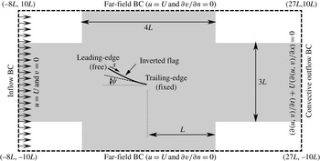
The computational domain and assumed boundary conditions.

Figure 2 shows the rectangular computational domain as well as the specified boundary conditions employed in this study. The initial position of the flag is a straight line extending from its leading edge to its trailing edge at
 $(L,0)$
. The flag may be inclined at an angle
 ${\it\psi}$
to the incoming flow but the value of
 ${\it\psi}$
is equal to
 $0^{\circ }$
unless noted otherwise. The majority of the simulations are conducted at a Reynolds number of
 $Re=200$
. This value is large enough to generate complex vortex-induced vibrations in the flag, but low enough to allow for a thorough sweep of the parameter space. However, one part of the study also examines the effect of Reynolds number on the configuration. A uniform velocity is assumed at all the boundaries except the outflow boundary, where a convective outflow boundary condition is used. A zero normal gradient boundary condition is used for pressure at all the boundaries.
The size of the computational domain is chosen to be
 $-8L\leqslant x\leqslant 27L$
and
 $-10L\leqslant y\leqslant 10L$
after a domain dependence study to ensure that further increase in domain size has no significant effect on the gross quantities (lift, drag, vibration amplitude and frequency) as well as the vortex topology in the vicinity of the flag. A uniform grid with 78 points is used to discretize the flag and the computational domain is discretized with
 $555\times 420$
points in the
 $x$
and
 $y$
directions, respectively. The grid density is increased in the region around the flag extending from
 $-L$
to
 $2L$
in the
 $x$
direction and
 $-1.5L$
to
 $1.5L$
in the
 $y$
direction (as shown by the a shaded area in figure 2) with grid sizes of
 ${\rm\Delta}x={\rm\Delta}y=0.0167L$
. The time step
 $t$
is chosen to be
 $0.00025L/U$
, which corresponds to a maximum Courant–Friedrichs–Lewy (CFL) number of approximately 0.04. In the numerical simulations we choose
 ${\it\kappa}_{p}=-2\times 10^{5}$
. Sensitivity tests conducted for the current system indicate that the chosen numerical parameters are adequate for the accuracy and stability of the simulations, and the maximum uncertainty introduced by these parameters is estimated to be less than 2 %.
2.6 Validation and verification
The accuracy and fidelity of the above formulation for flow and fluid–structure interaction has been assessed for a wide variety of canonical problems in the past (Shoele & Zhu Reference Shoele and Zhu2012, Reference Shoele and Zhu2013, Reference Shoele and Zhu2015; Shoele & Mittal Reference Shoele and Mittal2014). In particular, previous simulations of flow past a flexible flag have shown that the immersed boundary solver employed here accurately predicts vortex-dominated flows at the Reynolds numbers relevant to the current study. One verification study that is particularly relevant to the current work is the one in Shoele & Mittal (Reference Shoele and Mittal2014), where the flow-induced flutter of a flexible plate mounted behind a circular cylinder in a channel was simulated and the results compared to a study that employed a finite-element discretization (Turek & Hron Reference Turek and Hron2006) and another study that employed a sharp-interface immersed boundary method (Bhardwaj & Mittal Reference Bhardwaj and Mittal2012). The comparisons showed that the results generated by the current immersed boundary flow–structure interaction (FSI) solver were in very good agreement with these past studies, thereby verifying the fidelity of the current solver for an FSI problem similar to the one studied here. The details of these studies are provided in the references quoted above and will not be repeated here.
The new modelling component that is incorporated in the current study is the structural–electrical coupling of the piezoelectric beam. In order to test this module of the computational model, we employ the canonical cases of a thin piezoelectric plate with one end cantilevered, undergoing forced oscillations in the absence of an ambient fluid. The plate is actuated with a periodic heaving motion at its fixed end of the form
 $y_{0}=A_{0}\sin ({\it\omega}_{0}t)$
and the vertical deflection of its tip examined. Under the assumption of small deflection, where nonlinear effects can be neglected, and the base of the beam actuated with a periodic function, the vertical deflection of the beam can be written as
 $y(x,t)=\text{Re}[Y(x)\text{e}^{\text{i}{\it\omega}t}]$
, and we can combine (2.11) and (2.12) into
 $$\begin{eqnarray}\displaystyle Y_{xxxx}-{\it\kappa}({\it\omega}_{0})Y=0, & & \displaystyle\end{eqnarray}$$
where
 $$\begin{eqnarray}\displaystyle {\it\kappa}({\it\omega})={\it\omega}^{2}\frac{{U^{\ast }}^{2}}{M^{\ast }}\left[1+\frac{\text{i}{\it\alpha}^{2}{\it\beta}{\it\omega}}{1+\text{i}{\it\beta}{\it\omega}}\right]^{-1}, & & \displaystyle\end{eqnarray}$$
along with the boundary conditions at the free and cantilevered ends, which are
 $Y_{xxx}(1)=Y_{xx}(1)=Y_{x}(0)=0$
and
 $Y(0)=1$
. The ordinary differential equation (2.32) is solved analytically and the deflection of the beam at its tip is found to be
 $$\begin{eqnarray}\displaystyle A_{tip}=Y(1)=\frac{\cos \left(\sqrt[4]{{\it\kappa}({\it\omega}_{0})}\right)+\cosh \left(\sqrt[4]{{\it\kappa}({\it\omega}_{0})}\right)}{\cos \left(\sqrt[4]{{\it\kappa}({\it\omega}_{0})}\right)\cosh \left(\sqrt[4]{{\it\kappa}({\it\omega}_{0})}\right)+1}. & & \displaystyle\end{eqnarray}$$
The above then gives us an analytical solution of the coupled mechanical–electrical problem in the case of small deflection for a simple canonical case and we can obtain solutions for any choice of the electrical and structural parameters. The same problem can also be solved numerically by using our computational model.
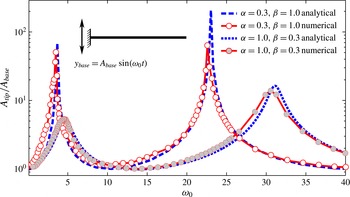
In figure 3, we compare our prediction of the fundamental frequency of the beam (with length
 $L$
) as well as the amplification factor of the tip oscillation with the analytical results for a configuration with
 $A_{0}/L=0.0025$
,
 $M^{\ast }=1$
and
 $U^{\ast }=1$
, but with two different electrical properties: one with
 ${\it\alpha}=0.3$
and
 ${\it\beta}=1$
, and the other with
 ${\it\alpha}=1.0$
and
 ${\it\beta}=0.3$
. The comparison shows that the computational method captures the overall trends quite well and does a reasonable job of predicting the resonance frequencies of the coupled piezo–structural system. A trend that emerges from the comparison is that the peaks from the simulations are shifted down and slightly to the right of those predicted by the analytical model. Further examination of this shift in the computational predictions is due to nonlinear effects. Note that even though the input deflection is small, the deflection in the beam at resonance can be amplified by factors ranging from approximately 10 to 200, and these are large enough to interject nonlinear effects into the dynamics of this beam; these nonlinear effects are absent in the analytical solution but are present in the computational model, leading to the observed differences. Stanton et al. (Reference Stanton, Erturk, Mann, Dowell and Inman2012) showed that, for large deflections, the nonlinearity of the mechanical–electrical coupling term reduces the response amplitude at resonance and the inextensibility condition of the beam introduces a cubic nonlinearity in the bending stiffness, which shifts the response curves to the left. Thus, the above comparison provides some confidence in the fidelity of the piezo–structural coupling and also provides a preview of the non-negligible effect of this coupling on the dynamics of the flexible piezoelectric beam.
Spectrum of the amplification factor at the tip of the piezoelectric beam
 $(A_{tip}/A_{base})$
as a function of actuation frequency at the base of the beam. The dotted lines are the theoretical prediction for a small-deflection model and the solid line along with the symbols are the numerical results.

2.7 Key metrics for flag dynamics and performance
A variety of metrics are employed in order to characterize the dynamics of the flag as well as its energy harvesting performance. The mean deflection of the flag is defined by
 $\bar{{\it\theta}}=\tan ^{-1}(\bar{y}_{LE}/\bar{x}_{LE})$
, where
 $x_{LE}$
and
 $y_{LE}$
are the
 $x$
and
 $y$
locations of the leading edge of the inverted flag, respectively, and the overbar indicates a time average. The non-dimensional oscillation amplitude
 $A_{max}$
of the flag leading edge is defined as
 $$\begin{eqnarray}\displaystyle A_{max}=\frac{\sqrt{(x_{LE}^{\prime })^{2}+(y_{LE}^{\prime })^{2}}}{L}, & & \displaystyle\end{eqnarray}$$
where ‘primed’ values denote root-mean-square (r.m.s.). The mean value and r.m.s. are calculated over a period of approximately four vibration cycles once the system reaches a stationary state.
The energy harvested by the piezoelectric flag is equal to the instantaneous power dissipated in the piezo patches. Following Michelin & Doare (Reference Michelin and Doare2013), the harvested energy is calculated in terms of a power coefficient by normalizing the harvested power with
 ${\it\rho}U^{3}(2L)/2$
, which is the kinetic energy flux of the fluid in the region accessible to the flag:
 $$\begin{eqnarray}\displaystyle C_{P}=\frac{P}{{\it\rho}U^{3}L}=\frac{1}{{\it\beta}}\int _{0}^{1}V^{2}\,\text{d}s. & & \displaystyle\end{eqnarray}$$
This power coefficient can also be viewed as the aerodynamic efficiency of energy harvesting by the flag.
3 Results
3.1 Effects of inertia and bending stiffness
In this section, we focus on the roles of inertia and bending stiffness on the flag dynamics. For this part of the study,
 ${\it\alpha}$
and
 ${\it\beta}$
are assumed to be zero (there is therefore no coupling between the elastic and electrical responses of the flag) and three representative values of the non-dimensional inertia
 $M^{\ast }=0.1$
, 1 and 10 are chosen. These represent, respectively, flags that have inertia that is significantly higher than, similar to and much lower than that of the ambient fluid. For each value of
 $M^{\ast }$
, the coupled dynamics of the system are investigated for a range of bending stiffness as represented by
 $U^{\ast }$
. The Reynolds number for all of these cases is chosen to be 200. Based on our study of the effect of Reynolds numbers, which ranged from
 $Re=25$
to 800 (see appendix A), the overall dynamics of the flag are similar beyond a Reynolds number of approximately 100. The choice of
 $Re=200$
therefore provides a value that is high enough to explore the rich dynamics of the flag, while at the same time low enough to limit the computational expense of the large parameter exploration that is conducted here.
3.1.1 Symmetry of motion and oscillation amplitude
The overall response of the inverted flag to changes in
 $M^{\ast }$
and
 $U^{\ast }$
in the
 $\bar{{\it\theta}}{-}A_{max}$
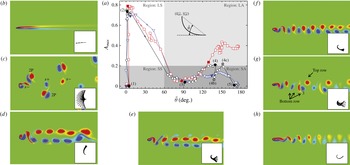
plane is shown in figure 4(a). The corresponding
 $\bar{{\it\theta}}$
and
 $A_{max}$
as well as drag and lift coefficients in the
 $M^{\ast }{-}U^{\ast }$
plane are shown in appendix B. The response of the flag can be qualitatively divided into four different regions, as presented with different shades and labelled SS, LS, SA and LA. In the region SS, both the mean deflection and the oscillatory amplitude of the inverted flag are small. In region LS, the flag has large, nearly symmetric oscillations making this region a good candidate for harvesting fluid kinetic energy. Region SA corresponds to flags with large mean deflections, but small oscillatory amplitudes. Finally, in region LA the flag has a large mean deflection and a sizeable oscillatory amplitude.
In case (1), which corresponds to the smallest value of
 $U^{\ast }~(=1.0)$
shown in figure 4(b), the inverted flag bends very slightly in one direction and shows negligible vibration around this state. Its response is therefore primarily placed in the region SS of the
 $\bar{{\it\theta}}{-}A_{max}$
plane (figure 4). We note that despite a hundred-fold change in
 $M^{\ast }$
, all cases with
 $U^{\ast }=1.0$
behave in a similar manner. The inset for this case shows that the vortex sheet remains attached to the body and extends downstream in an approximately straight line.
(a) Performance map showing the response of the inverted flag inside the plane of the mean angle of the leading edge
 $\bar{{\it\theta}}$
, and oscillatory amplitude of the leading edge
 $A_{max}$
for
 $M^{\ast }=0.1$
(squares, red), 1 (circles, black) and 10 (triangles, blue) for the baseline case with
 ${\it\psi}=0^{\circ }$
and
 $Re=200$
. The arrows show the direction of the
 $U^{\ast }$
increase, which changes from 1 (very stiff) to 25 (very flexible). The performance map constitutes a total of 160 simulations. The response can be qualitatively divided into four regions: SS, small symmetric oscillation; LS, large symmetric oscillation; SA, small asymmetric oscillation; and LA, large asymmetric oscillation. Distinct oscillatory states identified in the plots for
 $M^{\ast }=1$
are labelled from (1) to (5). In addition, for selected cases in each state, the corresponding cases with similar
 $U^{\ast }$
, but different
 $M^{\ast }$
, are also presented with filled symbols. Selected cases: (b) case (1) with
 $U^{\ast }=1.0$
; (c) case (2) with
 $U^{\ast }=2.2$
; (d) case (3) with
 $U^{\ast }=3.6$
; (e) case (4) with
 $U^{\ast }=7$
; (f) case (4b) with
 $U^{\ast }=8.5$
; (g) case (4c) with
 $U^{\ast }=13$
; (h) case (5) with
 $U^{\ast }=16$
.

Case (2) corresponds to
 $U^{\ast }=2.2$
, which may be viewed as a flag with bending stiffness
 $k_{b}$
nearly five times lower than in case (1). For this case, the flag shows very large oscillatory amplitude while its mean deflection remains very small (hence, this is in region LS). Similar to region SS, we observe that the response curves of all
 $M^{\ast }$
cases in this region also approximately collapse onto each other. Moreover, from figure 4(c) it appears that the flow field of a typical case in this state consists of two distinct vortex streets: a street made of vortex pairs (2P mode), which spreads out with a constant angle as it moves downstream, and a Kármán vortex street with broadly spaced positive and negative vortices (2S mode) along the wake centreline. A closer examination of the vortex shedding for case (2) shows that, as the flag’s leading edge moves away from the centre, a new vortex starts emerging from the trailing edge. The strength of this vortex increases as the flag approaches the peak of its deformation, but at the same time, when the flag decelerates, an opposite-sign vortex appears from the leading edge. The leading-edge vortex pairs with the vortex that has already been released from the trailing edge, while the remaining vortices created at the trailing edge during the return period of the flag from its maximum excursion combine into a secondary weaker vortex sheet behind the flag. It is noted that the amplitude of the motion peaks at approximately
 $0.8L$
in this region irrespective of the value of
 $M^{\ast }$
.
Case (3) with
 $U^{\ast }=3.6$
lies in region SA where we observe a transition to a mode with a mean deflection of
 $\bar{{\it\theta}}\sim 90^{\circ }$
and a small amplitude of oscillation (figure 4
d). The vortices from the trailing and leading edges are shed alternately within a short time interval but at well-separated vertical positions. The wake is therefore made of two nearly parallel vortex streets and, in each of these streets, the shed vortices are densely packed along a straight line. This arrangement of vortex sheets however becomes unstable at points further in the wake, causing reorganization into a new configuration.
With a further increase in
 $U^{\ast }$
beyond approximately 4.5, there is a continuous increase in
 $\bar{{\it\theta}}$
up to nearly
 $180^{\circ }$
, indicating almost complete inversion of the leading edge. However, unlike all the other regimes, the value of
 $M^{\ast }$
has a significant effect on the oscillation amplitude in this regime, with the lighter flags exhibiting a large amplitude of vibration. Thus, the overall response is divided into regions SA and LA. The variation in the oscillatory amplitude in this range is a consequence of changes in the dominant flapping mode shape; this point is made clear by examining the deformation pattern and flow field for three sample cases (marked with (4), (4a) and (4b) with
 $U^{\ast }=7$
,
 $8.5$
and
 $13$
, respectively, in figure 4
a, and shown in figure 4
e–g) that represent large variations in the vibration amplitude with
 $U^{\ast }$
. We note that this sensitivity of the flapping mode to flag inertia is typical of a conventional flag that is fixed at its leading edge (Connell & Yue Reference Connell and Yue2007; Shelley & Zhang Reference Shelley and Zhang2011).
In case (4) the flag bends significantly and oscillates with an amplitude larger than in case (3). In this case, the vortex that sheds from the leading edge is stretched by the motion of the leading edge and penetrates the vortex street from the trailing edge. This results in a weaker secondary vortex street in addition to the dominant vortex street. At
 $U^{\ast }=8.5$
, the oscillatory amplitude of the flag decreases and its dynamic deflection mainly concentrates near the leading edge while it bends more towards the positive
 $x$
axis. The wake consists of a typical Kármán vortex street reminiscent of a canonical bluff body. With further increase in
 $U^{\ast }$
to
 $13$
, the flag again shows a larger oscillation; however, in contrast to case (4) where the deflection is limited to the flag tip, in this case, there is a large longitudinal motion of the entire flag. The flow field in this case is also quite different from the previous cases and consists of an asymmetric vortex street with a set of three vortices at the bottom and a single vortex at the top of the street (figure 4
g). It seems that one of the two subsequent vortices shed from the trailing edge interacts strongly with the two nearby opposite-sign vortices that originated from the leading edge to create a triple-vortex cluster in the lower street.
For case (5), which corresponds to
 $U^{\ast }=16$
, the flag bends totally in the opposite direction but is nearly stationary (figure 4
h). However, heavier flags (for instance
 $M^{\ast }=0.1$
) for this value of
 $U^{\ast }$
are found to flap with a relatively large amplitude. The vortex shedding for case (5) exhibits behaviour similar to that for case (4b) in that it shows a very symmetric Kármán vortex street: vortices in the wake on one side from the trailing edge and on the other from an intermediate point along the flag with the maximum vertical excursion (Shoele & Zhu Reference Shoele and Zhu2010).
It is useful to compare and contrast the trends in flag dynamics observed here with the experiments of Kim et al. (Reference Kim, Cossé, Cerdeira and Gharib2013). First, we note that, despite the roughly three orders of magnitude higher Reynolds number (experiments are in the
 $Re\approx 10^{5}$
range) and the small
 $({\approx}1)$
aspect ratio of the flag in the experiments, the overall behaviour observed here has a number of similarities to that observed in the experiments. First, the state of large symmetric vibrations is observed to occur for a range of intermediate values of
 $U^{\ast }$
. For the simulations this range extends from
 $U^{\ast }\approx 1.4$
to 2.6, whereas in the experiments this range was from 1.8 to approximately 3.0 (see figure 2a in Kim et al. (Reference Kim, Cossé, Cerdeira and Gharib2013)). This quantitative difference could be due to Reynolds-number difference or 3D effects, or both. We note, however, that the maximum amplitude of the flag in this mode of vibration, which is a key parameter for energy harvesting, is also remarkably similar
 $(A_{max}/L\approx 0.8)$
between the experiments and current simulations. Thus, the most energetic flutter mode that is relevant for energy harvesting is reasonably well characterized by the current model.
Below this range of
 $U^{\ast }$
, both the experiments and simulations show a small asymmetric deflection with nearly zero vibration amplitude; above this range, both studies exhibit a large asymmetric deflection with a small amplitude of flutter. Kim et al. (Reference Kim, Cossé, Cerdeira and Gharib2013) suggested (but did not show) that further increases in
 $U^{\ast }$
would result in the flag bending all the way
 $(180^{\circ })$
into the streamwise direction and the flag would subsequently flap like a conventional flag. Our simulations, which extend far into this range of highly flexible flags, suggest a richer behaviour of flags in this regime; this ranges from flutter that is limited to the tip of the flag, and large-scale streamwise-dominated movements of the entire flag, to cessation of the vibration for some flags at the highest values of
 $U^{\ast }$
. However, as shown in appendix A, increase in the Reynolds number generally tends to energize more the flutter of the flag at these high
 $U^{\ast }$
values.
The effect of
 $M^{\ast }$
on the flag motion is another area where comparisons to the experiments are useful. One key observation in the experiments of Kim et al. (Reference Kim, Cossé, Cerdeira and Gharib2013) was that the dynamics of flags in the symmetric flapping mode was mostly independent of the mass ratio of the flag over a large range of this parameter. The current simulations are very much in line with this observation, although, in the regime of high
 $U^{\ast }$
, which was not covered in these previous experiments, the flag flutter does exhibit a more significant dependence on
 $M^{\ast }$
. The independence of vibration amplitude
 $A_{max}$
on the inertia of the flag provides an opportunity to design a system that could potentially deliver similar performances in different fluid media.
The region from
 $U^{\ast }=1.4$
to
 $2.6$
, where all flags in the current model deliver near-maximum
 $A_{max}$
with
 $\bar{{\it\theta}}\sim 0$
, is most promising for energy harvesting. The large oscillation amplitude and the low sensitivity of
 $A_{max}$
to
 $M^{\ast }$
and
 $U^{\ast }$
when the flag oscillates in this mode are unique properties of the inverted flag compared to the conventional flag with a fixed leading edge (Kim et al.
Reference Kim, Cossé, Cerdeira and Gharib2013), and make the current system an attractive candidate for harvesting energy. This idea is explored in detail in the latter half of the paper.
3.1.2 Frequency response
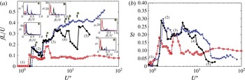
Figure 5(a) shows the frequency response of the flag for various inertia and stiffness values. The frequency shown here is identified as the dominant frequency in the spectra of
 ${\it\theta}$
. Cases (1)–(5) identified in figure 4 are also marked on these frequency plots. First, we note that all cases exhibit a non-continuous variation in the frequency with
 $U^{\ast },$
and this is clear evidence of the complex mode transitions exhibited by the flag. Second, while the
 $M^{\ast }=1.0$
and 10 flags show a very similar frequency response for
 $U^{\ast }<5$
, the heaviest flag
 $(M^{\ast }=1)$
is quite distinct in its response. In particular, over a large range of
 $U^{\ast }$
, its frequency is relatively unaffected by
 $U^{\ast }$
and stays at a non-dimensional value of approximately 0.8, indicating that flag inertia dominates the dynamics of this flag.
Dependence of (a) the flag dominant frequency and (b) the vibrational Strouhal number
 $(St=f\,Y/U)$
on
 $U^{\ast }$
for the flag with
 $M^{\ast }=0.1$
(squares, red), 1 (circles, black) and 10 (triangles, blue). The frequency spectra for the tip vibration are shown for selected cases in the insets in (a).

Flow-induced flutter results from a complex interaction between the intrinsic time scales (natural frequencies) of the flag and the time scales associated with the flow. In order to gain some insight into this interaction, we re-compute the frequency by using the length scale
 ${\rm\Delta}Y$
associated with the wake of the flag;
 ${\rm\Delta}Y$
is defined as the maximum frontal projection presented by the flag to the flow, and is computed based on the mean deflection as well as the vertical oscillation amplitude of the stationary state of the flag. In figure 4(b) we have plotted the variation of this Strouhal number versus
 $U^{\ast }$
and we note the following. First, this scaling shows an even better collapse for the
 $M^{\ast }=1.0$
and 10 flags, indicating that the dynamics of these two flags are fundamentally similar, despite a 10-fold difference in inertia. Furthermore, over a fairly large range of
 $U^{\ast }$
from approximately 3 to 9, the Strouhal number of the flag calculated based on this length scale is approximately 0.2, which is close to the most unstable frequency for drag-producing bodies (Williamson Reference Williamson1996) as well as flapping foils (Koochesfahani Reference Koochesfahani1989; Triantafyllou, Triantafyllou & Gopalkrishnan Reference Triantafyllou, Triantafyllou and Gopalkrishnan1991). Further noting that
 $1/U^{\ast }$
may be viewed as the inverse of the structural frequency, a value of
 $U^{\ast }\sim 5$
, which is roughly in the middle of this range, would match the most unstable wake frequency. Thus, in the range of
 $U^{\ast }$
between 3 and 9, the lighter flags exhibit a ‘lock-on’ behaviour that is typical for cases involving flow-induced vibration (Blevins Reference Blevins1977; Paidoussis, Price & De Langre Reference Paidoussis, Price and De Langre2010). We also note that the heaviest flag continues to show a lack of collapse with the other cases, reaffirming the dominant effect of inertia in this case.
From the viewpoint of energy harvesting, the range of
 $U^{\ast }$
between 1.5 and 2.5, where all cases exhibit large symmetric oscillations, is particularly interesting, and we examine the three flags in more detail for
 $U^{\ast }=2$
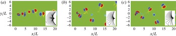
, which is in the middle of this range. Figure 6 shows the vortex shedding for these cases, with insets showing the vibration mode (snapshots at equal time intervals). We note that the overall mode of vibration and amplitude are quite similar for all cases, although the heaviest flag exhibits the most bending. However, despite this similarity, the wake dynamics of the heavy flag is fundamentally different from the other two. The
 $M^{\ast }=0.1$
flag sheds thee vortices at each half-stroke (a dipole from the flag leading edge and a single vortex from the trailing edge) and generates a meandering vortex street, whereas the other two cases shed a vortex dipole from the leading edge at the end of each half-strokes, and these generate an oblique, bifurcating wake observed for flapping foils (Dong et al.
Reference Dong, Bozkurttas, Mittal, Madden and Lauder2010). This difference is due to the significantly lower frequency of the heavy flag (
 $St=0.13$
for
 $M^{\ast }=0.1$
versus
 ${\sim}0.22$
for the other two lighter flags), which allows sufficient time for the vortex to develop and shed from the trailing edge.
Vorticity contours of a flag with
 $U^{\ast }=2$
for different
 $M^{\ast }$
values: (a)
 $M^{\ast }=0.1$
; (b)
 $M^{\ast }=1.0$
; (c)
 $M^{\ast }=10$
. The insets show the mode of flutter.

3.2 Dependence on the inclination angle,
${\it\psi}$

The appearance of highly asymmetric modes in the vibration of the inverted flag suggest that this configuration could be more sensitive to asymmetries in the direction of flow relative to the axis of the flag than the conventional flag. In this section, we explore this sensitivity by changing the initial inclination angle
 ${\it\psi}$
of the inverted flag. For this study,
 $M^{\ast }$
is fixed to an intermediate value of 1.0 and the effect of
 ${\it\psi}$
on the dynamics of the flag is studied for
 $U^{\ast }$
ranging from 1 to 10, a region that is of interest for energy harvesting application. Furthermore, the coefficients
 ${\it\alpha}$
and
 ${\it\beta}$
are assumed to be zero for this component of the study also.
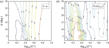
Figure 7(a,b) shows the contour plots of
 $(\bar{{\it\theta}}{-}{\it\psi})$
and percentage change in
 $A_{max}$
over the baseline
 $({\it\psi}=0)$
case in the
 ${\it\psi}{-}U^{\ast }$
plane. It is noted that, for the most part, the contours in these plots are vertically inclined, which suggests that the performance is relatively unaffected by the inclination of the flag to the wind. However, in the very narrow range from
 $U^{\ast }\sim 1.5$
to
 $2.5$
, where the baseline flag exhibits large symmetric vibrations, the mean deflection of the flag as well as the vibration amplitude diminish quite noticeably as
 ${\it\psi}$
is increased beyond
 $15^{\circ }$
. Since the large symmetric vibration state is expected to be most conducive to energy harvesting (this is explored in the next section), the indication from the current study is that, while the performance of the inverted flag would be insensitive to small
 $({<}15^{\circ })$
misalignments between the flag axis and wing direction, larger misalignments could significantly compromise the flag performance.
Dependence of (a)
 $\bar{{\it\theta}}$
and (b)
 $A_{max}$
on
 $U^{\ast }$
and
 ${\it\psi}$
for the flag with
 $M^{\ast }=1$
.

3.3 Energy harvesting and effect of piezoelectric parameters
The focus of this section is on assessing the effect of the piezoelectric parameters: the piezo–mechanical coupling parameter
 ${\it\alpha}$
, and the piezoelectric tuning parameter
 ${\it\beta}$
. For this part of the study we retain the focus on the
 $U^{\ast }=2$
,
 $M^{\ast }=1$
case, which is representative of the large symmetric oscillation state that is most promising for energy harvesting. The coupling parameter
 ${\it\alpha}$
is dependent on the piezo material characteristics and it is particularly difficult to modify this parameter. Widely available piezoelectric materials such as PZT (lead zirconate titanate) exhibit
 ${\it\alpha}\sim 0.3$
, with values of
 ${\it\alpha}\sim 0.5$
achievable with improved material design (Michelin & Doare Reference Michelin and Doare2013). As pointed out by Michelin & Doare (Reference Michelin and Doare2013), even larger
 ${\it\alpha}$
values could be achieved in the near future and, given this, we test the performance of the inverted flag for the values of
 ${\it\alpha}=0.3$
,
 $0.5$
and
 $0.9$
.
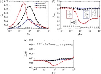
The dependence of harvested energy and oscillation amplitude of the inverted flag on the piezoelectric tuning parameter
 ${\it\beta}$
for three values of the coupling parameter
 $({\it\alpha}=0.3,~0.5,~0.9)$
are shown in figure 8(a,b). First, it is observed that the peak power coefficient increases with
 ${\it\alpha}$
. Since
 $\bar{C}_{P}$
also denotes the aerodynamic energy harvesting efficiency, the numbers above indicate that efficiencies ranging up to approximately 7 % are achieved. For comparison, the energy harvesting performance of a conventional flag with a clamped leading edge is also included in the plot. For this case, we have selected
 $M^{\ast }=1.0$
and
 ${\it\alpha}=0.5$
, and
 $U^{\ast }=14.5$
is selected based on the optimal case reported in Michelin & Doare (Reference Michelin and Doare2013). The simulations indicate that the peak
 $\bar{C}_{P}$
for the conventional flag is approximately an order of magnitude lower than that for the corresponding inverted flag. Furthermore, the performance of the inverted flag significantly exceeds that of the conventional flag over a large range of the parameters considered here.
The maximum energy harvesting at
 ${\it\beta}{\it\omega}\sim O(1)$
, where
 ${\it\omega}=2{\rm\pi}fL/U$
is the dominant angular frequency for the flag, is not surprising as this coefficient represents the ‘resonance’ between the flow time scale and the time scale of the electric circuit
 $c/{\it\varsigma}$
. In fact, it has been shown before (Michelin & Doare Reference Michelin and Doare2013), as well as in our simulation of such a flag, that optimal forcing of the piezoelectric flag with a clamped leading edge occurs at
 ${\it\beta}{\it\omega}\sim O(1)$
; this simple resonance condition therefore seems to apply to the inverted flag also.
Evolution of (a) harvested energy,
 $\bar{C}_{P}$
, (b) oscillation amplitude of the leading edge,
 $A_{max}$
, and (c) the flag dominant frequency with
 ${\it\beta}{\it\omega}$
for different values of
 ${\it\alpha}$
. The plots correspond to
 $M^{\ast }=1$
and
 $U^{\ast }=2$
. For comparison, results of a conventional flag with a fixed leading edge with
 $M^{\ast }=1$
,
 ${\it\alpha}=0.5$
and
 $U^{\ast }=14.5$
are also plotted (grey squares, dotted line). The insets in (b) show mode shapes for the cases with maximum
 $\bar{C}_{P}$
marked with filled symbols.

We explore further the dynamics of the flag for these various cases. Figure 8(b) shows the amplitude and mode of vibration for some selected cases. We note first that, for the entire set of cases simulated here, the inverted flag exhibits symmetric or nearly symmetric vibrations. Thus, variations in the piezo parameters do not change the vibratory mode of the flag. The amplitude of the flag flutter is found to be relatively insensitive to
 ${\it\beta}{\it\omega}$
for
 ${\it\alpha}=0.3$
and 0.5. This relative insensitivity of the flag amplitude to the piezo parameters is, however, lost for
 ${\it\alpha}=0.9$
where the amplitude is observed to fall to approximately 50 % of its maximum value as
 ${\it\beta}{\it\omega}$
is changed.
Figure 8(c) shows the dependence of oscillation frequency with respect to
 ${\it\beta}{\it\omega}$
, for the three values of
 ${\it\alpha}$
. For
 ${\it\alpha}=0.3$
and 0.5, the oscillation frequency is nearly constant and only changes slightly in the range
 $1<{\it\beta}{\it\omega}<5$
. The frequency for the case with
 ${\it\alpha}=0.9$
, however, shows significant changes; it initially decreases to about half its baseline value but then rises rapidly beyond
 ${\it\beta}{\it\omega}\sim 1$
and reaches values comparable to the other
 ${\it\alpha}$
cases. Thus, except for the largest
 ${\it\alpha}~({\it\alpha}=0.9)$
, the oscillation frequency remains approximately constant with
 ${\it\beta}{\it\omega}$
, and hence is almost independent of
 ${\it\beta}$
. This robustness in the response of the inverted flag coupled with a relatively high energy harvesting efficiency is an attractive property of these flags.
The scaling of the energy harvesting performance with the dynamics of the flag can also be examined via a dimensional analysis of the governing equations. Assuming that the dominant mode of vibration of the flag in state (2) resembles the first mode of vibration of the flag, its curvature amplitude is proportional to
 $A_{max}$
(i.e.
 $\partial ^{2}\boldsymbol{X}/\partial s^{2}\boldsymbol{\cdot }\boldsymbol{n}\sim -{\it\Upsilon}(s)A_{max}$
, with
 ${\it\Upsilon}(s)$
being a non-dimensional function depending on the shape of the dominant mode shape of the flag). Therefore, the energy equation of the flag in the frequency domain can be expressed as
 $$\begin{eqnarray}\displaystyle (\text{i}{\it\beta}{\it\omega}+1)\hat{V}_{{\it\omega}}\sim \frac{{\it\alpha}{\it\beta}\sqrt{M^{\ast }}}{U^{\ast }}(\text{i}{\it\omega}{\it\Upsilon}A_{max}), & & \displaystyle\end{eqnarray}$$
where
 ${\it\omega}=2{\rm\pi}fL/U$
is the dominant non-dimensional vibrational angular frequency of the flag, and
 $V_{{\it\omega}}$
is the amplitude of the
 $V$
component with frequency
 ${\it\omega}$
. Therefore,
 $$\begin{eqnarray}\displaystyle {\hat{V}_{{\it\omega}}}^{2}\sim \frac{{\it\alpha}^{2}M^{\ast }}{U^{\ast ^{2}}}\frac{({\it\beta}{\it\omega})^{2}}{({\it\beta}{\it\omega})^{2}+1}({\it\Upsilon}A_{max})^{2} & & \displaystyle\end{eqnarray}$$
and from
 $\bar{C}_{P}\sim (1/{\it\beta})\int _{0}^{1}\hat{V}^{2}\,\text{d}s$
, and knowing that the flag has only one dominant frequency in its state (2) of vibration,
 $$\begin{eqnarray}\displaystyle \bar{C}_{P} & {\sim} & \displaystyle \frac{1}{2{\it\beta}}\int _{0}^{1}{\hat{V}_{{\it\omega}}}^{2}\,\text{d}s\sim \frac{1}{{\it\beta}}\frac{{\it\alpha}^{2}M^{\ast }}{U^{\ast ^{2}}}\frac{({\it\beta}{\it\omega})^{2}}{({\it\beta}{\it\omega})^{2}+1}\,A_{max}^{2}\frac{1}{2}\int _{0}^{1}{\it\Upsilon}^{2}\,\text{d}s\nonumber\\ \displaystyle & = & \displaystyle \frac{1}{{\it\beta}}\frac{{\it\alpha}^{2}M^{\ast }}{U^{\ast ^{2}}}\frac{({\it\beta}{\it\omega})^{2}}{({\it\beta}{\it\omega})^{2}+1}\,A_{max}^{2}{\it\Upsilon}_{P},\end{eqnarray}$$
where
 ${\it\Upsilon}_{P}=(1/2)\int _{0}^{1}{\it\Upsilon}^{2}\,\text{d}s$
is a non-dimensional coefficient based on the observed mode shape of the flag. For very small and very large values of
 ${\it\omega}{\it\beta}$
, we can approximate the above expression to
 $$\begin{eqnarray}\displaystyle \bar{C}_{P}\sim \left\{\begin{array}{@{}ll@{}}\displaystyle \frac{{\it\alpha}^{2}M^{\ast }}{U^{\ast ^{2}}}{\it\beta}{\it\omega}^{2}A_{max}^{2}{\it\Upsilon}_{P} & \text{for}\;{\it\omega}{\it\beta}\ll 1,\\ \displaystyle \frac{{\it\alpha}^{2}M^{\ast }}{U^{\ast ^{2}}}\frac{1}{{\it\beta}}A_{max}^{2}{\it\Upsilon}_{P} & \text{for}\;{\it\omega}{\it\beta}\gg 1.\end{array}\right. & & \displaystyle\end{eqnarray}$$
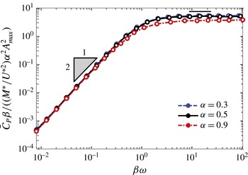
The above scaling laws can now be examined using the current simulation results. Figure 9 shows plots of
 $\bar{C}_{P}{\it\beta}/((M^{\ast }/U^{\ast ^{2}}){\it\alpha}^{2}A_{max}^{2})$
versus
 ${\it\beta}{\it\omega}$
for the different cases; and as predicted by the above scaling arguments, all cases scale with
 $({\it\beta}{\it\omega})^{-2}$
at small
 ${\it\beta}{\it\omega}$
and approach a constant value for large values of
 ${\it\omega}{\it\beta}$
, respectively. In the case of
 ${\it\alpha}=0.9$
for
 ${\it\beta}{\it\omega}\gg 1$
, the flag is highly damped; consequently, the asymptotic value of
 $\bar{C}_{P}{\it\beta}/((M^{\ast }/U^{\ast ^{2}}){\it\alpha}^{2}A_{max}^{2})$
in this case is lower than in the other cases. Notwithstanding this, the analysis and the results indicate that such scaling procedures could be used to determine the optimal range of
 ${\it\beta}$
and
 ${\it\alpha}$
as well as to estimate the power output for given electrical parameters.
Dependence of
 $\bar{C}_{P}{\it\beta}/((M^{\ast }/U^{\ast 2}){\it\alpha}^{2}A_{max}^{2})$
on
 ${\it\omega}{\it\beta}$
for various values
 ${\it\alpha}$
and
 ${\it\beta}$
. For all these cases,
 $M^{\ast }=1$
and
 $U^{\ast }=2$
.

4 Conclusions
In the present study, the coupled fluid–solid–electric dynamics of a self-excited 2D piezoelectric flag with a free leading edge and a fixed trailing edge, resembling an inverted flag, were investigated to determine the performance of this device as an energy harvesting mechanism. The material of the flag, which is modelled as a resistive circuit consisting of continuous infinitesimal piezoelectric patches on the surfaces of the flag, converts bending deformation into an electric current. A new implicit immersed boundary formulation is developed to solve the coupled fluid–solid–electric interaction problem using a detailed dynamical model for the flag dynamics, the piezoelectric circuit and the coupling mechanism between the electrical and mechanical domains.
The initial part of the study focused on a comprehensive examination of fluid physics and flag dynamics for different inertia
 $(M^{\ast })$
and bending stiffness
 $(U^{\ast })$
. The simulations show that the dynamic response of the flag exhibits a variety of distinct states, including symmetric as well as asymmetric flutter, but the state with large symmetric flapping is expected to be most conducive for energy harvesting. Similar to the previous experimental observations (Kim et al.
Reference Kim, Cossé, Cerdeira and Gharib2013), in the current 2D model this state is achieved in a certain range of bending stiffness, irrespective of the bending inertia, thereby indicating that the dynamics of the flag in this state are driven primarily by vortex shedding, with inertia only playing a minor role. The near wake for this state consists of two dominant vortex streets: a primary 2P vortex street with two rows of vortex pairs that convect at large angles from the wake centreline, and a secondary 2S vortex street that emerges along the centreline behind the flag. Rescaling of the vortex shedding with the projected wake width suggests that, in a range of
 $U\ast$
from approximately 3 to 9, there is lock-on between the flag flutter and the vortex shedding associated with the instability of the wake. It is also shown that the dynamic response of the flag is relatively insensitive to the change in initial inclination angle with respect to the flow as long as the inclination is less than
 $15^{\circ }$
.
Finally, the simulations explored the energy harvesting efficiency of the inverted flag as a function of the piezoelectric coupling coefficient and the tuning ratio. It is found that the large symmetric flapping mode of the inverted flag is highly effective for energy harvesting and outperforms the classical piezoelectric flag cases with clamped leading edge and free trailing edge (Michelin & Doare Reference Michelin and Doare2013). It is also noted that the oscillation amplitude in this efficient state is not highly sensitive to realistic values of piezoelectric coupling parameter and tuning parameter. Our results therefore suggest that the inverted flag is a robust system with good predictability that can be used in the design of more predictable and hence more controllable energy harvesting mechanisms. In this regard, it is also shown that the energy harvesting performance follows a well-defined scaling law which depends on the tuning between the vibration time scale and the intrinsic time scale of the piezoelectric circuit.
Future work in this area should focus on overcoming the limitations of the current computational model, which include the use of 2D modelling, the assumption of continuous infinitesimal piezoelectric patches and the low Reynolds numbers employed here. It would be interesting to investigate the potential improvements in performance of the system through shape modification of the flag and the use of state-of-the-art power electronics in the piezoelectric system. Finally, the current modelling approach could be used to explore the application of the inverted flag in other applications such as flow sensors and convective heat transfer enhancement (see e.g. Shoele & Mittal Reference Shoele and Mittal2014).
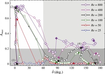
Performance map showing the response of the inverted flag inside the plane of the mean angle of the leading edge
 $\bar{{\it\theta}}$
, and oscillatory amplitude of the leading edge
 $A_{max}$
for different
 $Re$
assuming
 $M^{\ast }=1$
and
 ${\it\psi}=0^{\circ }$
. The arrows show the direction of the
 $U^{\ast }$
increase, which changes from 1 (very stiff) to 25 (very flexible).

Acknowledgements
The development of the fluid–structure interaction solver that forms the basis of this study was supported by the Air Force Office of Scientific Research under grant no. FA9550-13-0053 and NSF grant CBET-1357819. We also acknowledge support via a seed grant from E
 $^{2}$
SHI for this work.
Appendix A. Effect of Reynolds number
In this appendix, we provide results of our investigation of the effect of Reynolds number on the dynamics of the flag and the associated flow patterns. For this study, we have chosen a case with
 $M^{\ast }=1$
and
 ${\it\psi}=0^{\circ }$
and both
 $U^{\ast }$
and
 $Re$
are varied over
 $1<U^{\ast }<25$
and
 $25<Re<800$
, respectively. Figure 10 shows the flutter patterns for the various cases. For the lowest Reynolds number of 25, the flag shows very little flutter. However, beginning with
 $Re=50$
, a sizeable flutter response is noted for the flags for intermediate values of
 $U^{\ast }$
, and for Reynolds numbers beyond 100, the peak amplitude of flutter reaches a large value and stays nearly constant. Beyond this, the primary effect of the Reynolds number for the intermediate values of
 $U^{\ast }$
is to grow the region of
 $U^{\ast }$
over which large-amplitude flutter is observed. For the larger values of
 $U^{\ast }$
, the increase in
 $Re$
also has the effect of increasing the amplitude of flutter as well as the region of
 $U^{\ast }$
over which large-scale flutter is observed.
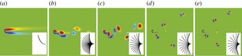
Vorticity contours of an inverted flag with
 $U^{\ast }=2$
,
 $M^{\ast }=1$
and
 ${\it\psi}=0^{\circ }$
for different
 $Re$
values: (a)
 $Re=25$
; (b)
 $Re=50$
; (c)
 $Re=100$
; (d)
 $Re=400$
; (e)
 $Re=800$
. The insets show the mode of flutter.

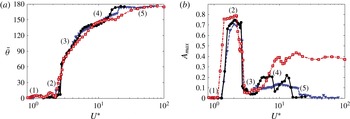
Dependence of (a) mean angle of the leading edge,
 $\bar{{\it\theta}}$
, and (b) oscillatory amplitude,
 $A_{max}$
, on the reduced velocity
 $U^{\ast }$
for
 $M^{\ast }=0.1$
(squares, red), 1 (circles, black) and 10 (triangles, blue).

Figure 11 shows the vortex patterns and flag mode shapes for the condition when it oscillates in its most energetic state of vibration (state (2) in figure 10). The figure shows the absence of vortex shedding for
 $Re=25$
, but the flutter modes are quite similar for
 $Re\geqslant 50$
. It is also noted that, for
 $Re\geqslant 100$
, the frequency of vibration of the energetic symmetric flutter state is very similar, and stays almost constant with increasing
 $Re$
. Furthermore, for
 $Re\geqslant 100$
, the vortices arrange into a characteristic bifurcating wake consisting of two streets of vortex dipoles. Given the above observations, it is concluded that, at least in this lower range of Reynolds numbers
 $(Re<1000)$
, the characteristic features of the flag dynamics and the vortex wake in the current model do not change much beyond
 $Re=100$
.
Appendix B. Flag dynamic response and fluid dynamic forces
In this section, we present detailed data on the flutter response of the flag as well as the fluid dynamic forces on the flag. These datasets are provided for the sake of completeness and for facilitating comparisons with other studies in the future. The dependence of
 $\bar{{\it\theta}}$
and
 $A_{max}$
on
 $U^{\ast }$
are presented in figure 12 for
 $M^{\ast }=0.1$
, 1 and 10. Different states are also marked in the figure.
The drag and lift coefficients of the flag are defined as
 $$\begin{eqnarray}\displaystyle C_{D}=\frac{F_{x}}{0.5{\it\rho}U^{2}L}\quad \text{and}\quad C_{L}=\frac{F_{y}}{0.5{\it\rho}U^{2}L}, & & \displaystyle\end{eqnarray}$$
where
 $F_{x}$
and
 $F_{y}$
are the drag and lift forces of the flag obtained by integrating the dimensional force density applied by the surrounding fluid on the flag (
 $-\boldsymbol{F}$
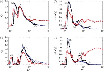
in (2.11)). Figure 13(a,b) shows the mean and standard deviations of the drag coefficients as a function of
 $U^{\ast }$
for
 $M^{\ast }=0.1$
, 1 and 10 and figure 13(c,d) shows the corresponding curves for the lift coefficient.
Dependence of (a) mean drag coefficient,
 $\bar{C}_{D}$
, (b) standard deviation of
 $C_{D}$
, (c) mean lift coefficient,
 $\bar{C}_{L}$
, and (b) standard deviation of
 $C_{L}$
on
 $U^{\ast }$
for the flag with
 $M^{\ast }=0.1$
(squares, red), 1 (circles, black) and 10 (triangles, blue).