

1. Introduction
Modern structural biology techniques, in particular X-ray crystallography and nuclear magnetic resonance (NMR) spectroscopy, have revealed much of the inner workings of biology at atomic resolution. However, these views have been largely restricted to states that are highly populated, homogeneous, static (especially for crystallography), and of relatively modest size (especially for NMR). However, many biological processes proceed through intermediate states that are short lived and comprise only a small fraction of the overall population of a molecular system at equilibrium; thus, they are invisible to conventional structural methods. These states, which constitute local minima above the global minimum on the free-energy landscape of a macromolecule (Bryngelson & Wolynes, Reference Bryngelson and Wolynes1987; Bryngelson et al. Reference Bryngelson, Onuchic, Socci and Wolynes1995; Miyashita et al. Reference Miyashita, Onuchic and Wolynes2003, Reference Miyashita, Wolynes and Onuchic2005; Onuchic et al. Reference Onuchic, Lutheyschulten and Wolynes1997; Wolynes, Reference Wolynes2005), include macromolecular encounter complexes, protein-folding intermediates, and states involved in conformational selection and enzyme catalysis (Clore, Reference Clore2011; Sekhar & Kay, Reference Sekhar and Kay2013). Other elusive states include large (~1 MDa or larger) macromolecular assemblies, especially those that are dynamic and/or heterogeneous, which include intermediates in some protein aggregation processes.
The methods available for characterizing biological molecules at atomic resolution, X-ray crystallography and conventional NMR spectroscopy, are generally incapable of probing the structures of sparsely populated or large, heterogeneous states. If well diffracting crystals are available, X-ray crystallography offers the most precise view into the structure of a protein at atomic resolution, although it offers only limited insight into its dynamics; the result is generally a single structure – or a family of closely related structures – which represents the most stable conformation within the constraints of the crystal lattice and the major population of the system of interest. Slight variations in structure can be seen between crystals and between protein chains within a crystal, and some side chains display multiple rotamers, although these can reflect crystal-packing artifacts. Crystallographic temperature factors (B-factors) can be interpreted as probes of local picosecond/nanosecond dynamics (Rueda et al. Reference Rueda, Ferrer-Costa, Meyer, Perez, Camps, Hospital, Gelpi and Orozco2007), although they also reflect crystallographic heterogeneity. More recently, new approaches to systematically interpret lower intensity signals in electron density maps (0·3–1σ) (Fraser et al. Reference Fraser, Clarkson, Degnan, Erion, Kern and Alber2009) or to fit X-ray diffraction data to an ensemble of structures (Burnley et al. Reference Burnley, Afonine, Adams and Gros2012) have offered more rigorous means to explore protein dynamics and minor states by X-ray crystallography.
Conventional structure determination by NMR relies on interpretation of interproton distance restraints derived from nuclear Overhauser effects (NOEs) and dihedral angle restraints derived from J couplings (Clore & Gronenborn, Reference Clore and Gronenborn1998). The addition of long-range orientational restraints from residual dipolar couplings (RDCs) to this repertoire has further improved the breadth and accuracy of structure determination by NMR (Tjandra et al. Reference Tjandra, Marquardt and Clore2000). Although these methods offer some insight into the dynamics of the molecule under study, they report almost solely upon the major population. More recently, paramagnetic relaxation enhancement (PRE) has been employed to provide long-range (up to ~35 Å under favorable circumstances) distance restraints by NMR as well as to gain insight into sparsely populated states (Bertini et al. Reference Bertini, Luchinat and Piccioli2001b; Clore & Iwahara, Reference Clore and Iwahara2009; Iwahara et al. Reference Iwahara, Schwieters and Clore2004a; Keizers & Ubbink, Reference Keizers and Ubbink2011; Otting, Reference Otting2010).
Other structural or biophysical methods are also capable of providing long-range distance information, although they often lack resolution and are generally incapable of observing minor states. Electron microscopy (EM) allows for lower-resolution structural characterization, generally of larger molecules, although modern single-particle cryo-EM has achieved resolutions better than 5 Å in very favorable cases (Baker et al. Reference Baker, Hryc, Zhang, Wu, Jakana, Haase-Pettingell, Afonine, Adams, King, Jiang and Chiu2013; Bartesaghi et al. Reference Bartesaghi, Merk, Borgnia, Milne and Subramaniam2013; Lyumkis et al. Reference Lyumkis, Julien, De Val, Cupo, Potter, Klasse, Burton, Sanders, Moore, Carragher, Wilson and Ward2013; Van Heel et al. Reference Van Heel, Gowen, Matadeen, Orlova, Finn, Pape, Cohen, Stark, Schmidt, Schatz and Patwardhan2000; Zhou, Reference Zhou2008). Although cryo-EM techniques can potentially ‘freeze out’ a range of molecular conformations, detection of minor species is made almost impossible by the need to average many individual particles. Atomic force microscopy (AFM) suffers from similar limitations. Other techniques for gaining structural insight include solution X-ray and neutron scattering, electron paramagnetic resonance (EPR) (in particular double electron–electron resonance (DEER)), and fluorescence (in particular Förster resonance energy transfer (FRET)). The latter results from the dipole–dipole coupling between two fluorophores and has an r −6 dependence on the distance between them, providing structural information in the range of 10–100 Å (Hillisch et al. Reference Hillisch, Lorenz and Diekmann2001). DEER, which results from the dipole–dipole coupling between two paramagnetic centers, has an r −3 dependence on the distance between them, providing structural information in the range of 20–60 Å (Altenbach et al. Reference Altenbach, Kusnetzow, Ernst, Hofmann and Hubbell2008; Klug & Feix, Reference Klug and Feix2008). These techniques do not suffer from the same molecular size limitations as NMR, but they have the additional major limitation that only a single pairwise distance can be measured per sample, whereas NMR offers hundreds to thousands of individual measurements per sample per experiment (Clore, Reference Clore2008).
Although conventional NMR techniques for biomolecular structure determination report on an ensemble of closely related structures describing a major state, a range of additional NMR techniques have been developed to characterize processes on timescales from picoseconds to hours/days (Fig. 1). Rapid local motions (ps–ns) can be probed by NMR relaxation methods (Clore et al. Reference Clore, Driscoll, Wingfield and Gronenborn1990a, Reference Clore, Szabo, Bax, Kay, Driscoll and Gronenbornb; Ishima & Torchia, Reference Ishima and Torchia2000; Kay et al. Reference Kay, Torchia and Bax1989; Peng & Wagner, Reference Peng and Wagner1994); often, 15N is used to monitor backbone motion, measuring T 1 and T 2 relaxation and 1H–15N heteronuclear NOE values (Kay et al. Reference Kay, Torchia and Bax1989), and the framework for analyzing these measurements by the model-free formalism is well established (Clore et al. Reference Clore, Driscoll, Wingfield and Gronenborn1990a; Kay et al. Reference Kay, Torchia and Bax1989; Lipari & Szabo, Reference Lipari and Szabo1982a, Reference Lipari and Szabob; Xia et al. Reference Xia, Deng and Levy2013). This methodology can be extended to describe larger-scale slower motions on the nanosecond timescale that are still faster than the reorientational time (Clore et al. Reference Clore, Driscoll, Wingfield and Gronenborn1990a, Reference Clore, Szabo, Bax, Kay, Driscoll and Gronenbornb). For larger proteins, the favorable spectral properties of methyl groups make the methyl 13C, 1H, and 2H nuclei good probes for dynamic processes in larger molecules (Igumenova et al. Reference Igumenova, Frederick and Wand2006; Ruschak & Kay, Reference Ruschak and Kay2010). Regardless, these experiments largely describe the rapid motion of the major state (or states) of a molecule. However, PRE offers the ability to characterize minor states in dynamic exchange with a major state on these fast timescales, as well as longer timescales up to ~250–500 μs.
NMR methods for characterizing a ‘dark’ state in exchange with a visible species. Simulated NMR spectra are shown for a resonance in exchange between two states (A and B) over a range of timescales. Shown from top to bottom are exchange lifetimes τ ex = 1 μs, 10 μs, 100 μs, 1 ms, 10 ms, 100 ms, and 1 s (k ex = 106–100 s−1). Spectra were simulated by solving the McConnell equations (Eqs. (16)–(20)) (McConnell, Reference Mcconnell1958) in MATLAB for a chemical shift difference between states of Δω/2π = 120 Hz (e.g. 2 ppm for 15N on a 600 MHz spectrometer). In this example, state A is the major state (p A = 75%), and state B is the minor state (p B = 25%). On the left, states A and B have identical intrinsic rates of transverse relaxation (R 20 = 10 s−1). On the right, state B has an enhanced intrinsic relaxation rate (R 2,B0 = 100 s−1), which could be due to a paramagnetic center or a slow rate of tumbling. In practice, p B could be much lower and R 2,B0 much larger, although less extreme values are used here for illustrative purposes. In the slow exchange regime (bottom), states A and B give rise to two separate peaks, although in practice state B may be invisible due to a low signal/noise ratio. In the fast exchange regime, a single peak is observed with a population-averaged chemical shift and apparent R 2. In the intermediate exchange regime (middle), the peaks undergo extreme chemical shift broadening, and the apparent R 2 is greatly enhanced due to R ex. Down the center of the figure, NMR methods for characterizing dark states are shown, with a rough range of timescales over which they can be applied. The three methods shown toward the right (PRE, lifetime line broadening (R llb), and DEST) are used to visualize a dark state with a greatly enhanced R 2 compared with the major state. The other methods shown, toward the left, depend on either a difference in chemical shift between states A and B (rotating frame relaxation dispersion (R 1ρ), CPMG relaxation dispersion, and CEST) or a difference in rates of hydrogen exchange.

Additional NMR techniques have been developed to monitor dynamics on the intermediate and slow timescales. Relaxation dispersion, using either Carr–Purcell–Meiboom–Gill (CPMG) (Carr & Purcell, Reference Carr and Purcell1954; Meiboom & Gill, Reference Meiboom and Gill1958) or rotating frame (R 1ρ) experiments, can characterize systems on the intermediate exchange timescale (~50–100 μs to 10 ms) (Korzhnev & Kay, Reference Korzhnev and Kay2008; Mittermaier & Kay, Reference Mittermaier and Kay2006; Palmer et al. Reference Palmer, Kroenke and Loria2001). The dynamics of systems in the intermediate exchange regime can also be characterized by analysis of resonance line shapes (Rao, Reference Rao1989). RDCs may also serve as a probe of dynamics on the μs timescale (Lange et al. Reference Lange, Lakomek, Fares, Schroeder, Walter, Becker, Meiler, Grubmueller, Griesinger and De Groot2008). Exchange processes taking place on slower timescales (ms–s) can be characterized by additional techniques, such as heteronuclear zz-exchange spectroscopy (Farrow et al. Reference Farrow, Zhang, Forman-Kay and Kay1994; Iwahara & Clore, Reference Iwahara and Clore2006b; Montelione et al. Reference Montelione, Winkler, Burton, Rinderknecht, Sporn and Wagner1989; Sahu et al. Reference Sahu, Clore and Iwahara2007; Wider et al. Reference Wider, Neri and Wuthrich1991), saturation transfer (Fawzi et al. Reference Fawzi, Ying, Torchia and Clore2010b, Reference Fawzi, Ying, Ghirlando, Torchia and Clore2011b, Reference Fawzi, Ying, Torchia and Clore2012; Vallurupalli et al. Reference Vallurupalli, Bouvignies and Kay2012) and hydrogen exchange (Bai, Reference Bai2006; Krishna et al. Reference Krishna, Hoang, Lin and Englander2004b). Processes that are even slower still (>s) can be studied by real-time NMR, where changes are monitored in sequentially acquired NMR spectra (Schanda & Brutscher, Reference Schanda and Brutscher2005).
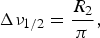
Thus, a wide range of techniques have been developed to study motions by NMR over a wide range of timescales; some of these techniques are applicable to characterizing exchange involving states that are invisible to conventional structural methods owing to their transient nature coupled with a low equilibrium population and/or large molecular weight. Detection and characterization of an otherwise invisible species is accomplished by amplifying the effect of the dark state on some NMR observable, so that its footprint is observed in measurements on the visible species. In many cases, the minor state is detected through an enhancement of spin relaxation. Two types of relaxation (the exponential return to equilibrium of the bulk magnetization in a sample after perturbation) occur in NMR experiments. Longitudinal relaxation describes the return to the equilibrium distribution of spin up and down states along the z-axis (the axis of the B 0 magnetic field) and is characterized by an exponential rate constant R 1 (or time constant T 1 = 1/R 1). Transverse relaxation describes a loss of coherence on the transverse xy-plane and is characterized by an exponential rate constant R 2 (or time constant T 2 = 1/R 2). Since this coherent xy signal is detected in an NMR experiment, the rate of transverse relaxation (R 2) determines the height and linewidth of each peak in the NMR spectrum (larger R 2 leads to broader peaks and lower peak heights):
 $${\rm \Delta} \nu _{{\rm 1}/{\rm 2}} = \displaystyle{{R_2} \over \pi}, $$
where Δν 1/2 is the linewidth (full-width at half-height) given in Hz. R 1, on the other hand, determines the necessary delay between individual scans in an NMR experiment (larger R 1 allows a faster rate of repetition).
Broadly speaking, NMR relaxation is of interest as an atomic-level probe of molecular dynamics; additionally, if a visible species is in exchange with an invisible species, under certain circumstances this can lead to an enhancement of the apparent R 2 relaxation rate observed for the visible species, allowing detection and characterization of the otherwise invisible state. The source of relaxation enhancement can vary, and the applicability of a given NMR experiment will depend on the timescale of the exchange event in question. Properties of the invisible state that can lead to such relaxation enhancements include slower tumbling due to a larger molecular weight (allowing study by dark state exchange saturation transfer (DEST) if exchange takes place on a slow (1 ms–1 s) timescale; Fawzi et al. Reference Fawzi, Ying, Ghirlando, Torchia and Clore2011b, Reference Fawzi, Ying, Torchia and Clore2012), different resonance frequencies (allowing study by relaxation dispersion if exchange takes place on an intermediate (100 μs–10 ms) timescale; Sekhar & Kay, Reference Sekhar and Kay2013), or closer proximity to an unpaired electron (allowing study by PRE if exchange takes place on a fast (<250–500 μs) timescale; Clore & Iwahara, Reference Clore and Iwahara2009). In the next section, we will survey some of these available NMR techniques for studying sparsely populated states, and in the following two sections, we will discuss two of these methods, PRE and DEST, in greater detail.
2. Survey of NMR methods for studying invisible states
Several different NMR experiments are available for studying invisible states over a range of different timescales (Clore, Reference Clore2011; Palmer et al. Reference Palmer, Grey and Wang2005; Sekhar & Kay, Reference Sekhar and Kay2013; Fig. 1); these include PRE (Clore & Iwahara, Reference Clore and Iwahara2009) and pseudocontact shifts (PCSs; Bertini et al. Reference Bertini, Giachetti, Luchinat, Parigi, Petoukhov, Pierattelli, Ravera and Svergun2010) (fast); rotating-frame (R 1ρ) (Palmer & Massi, Reference Palmer and Massi2006) and CPMG relaxation dispersion (intermediate) (Korzhnev & Kay, Reference Korzhnev and Kay2008); chemical exchange saturation transfer (CEST; Vallurupalli et al. Reference Vallurupalli, Bouvignies and Kay2012); DEST and lifetime line broadening (R llb) (slow) (Fawzi et al. Reference Fawzi, Ying, Ghirlando, Torchia and Clore2011b, Reference Fawzi, Ying, Torchia and Clore2012); and hydrogen exchange (very slow) (Englander et al. Reference Englander, Mayne and Krishna2007). The ability of these various methods to characterize an otherwise invisible species relies on enhancement of relaxation rates due to exchange with the invisible species. A major advantage of these NMR methods is that they offer high resolution (at least at the level of an individual residue – e.g. backbone amide – but often at atomic resolution). Many of these methods are built upon phenomena that were described decades ago (e.g. PRE (Solomon, Reference Solomon1955), CPMG (Carr & Purcell, Reference Carr and Purcell1954; Meiboom & Gill, Reference Meiboom and Gill1958), saturation transfer (Forsén & Hoffman, Reference Forsén and Hoffman1963)), but only through more recent methodological and technical advances have they become more widely applicable and has their utility for characterizing these otherwise invisible states been demonstrated.
2.1 Paramagnetic NMR
2.1.1 Types of paramagnetic observables
Unpaired electrons have dramatic effects on NMR spectra, and these paramagnetic effects are useful both as long-distance structural restraints and as probes of sparsely populated species. Here we will discuss two fundamental types of paramagnetic phenomena in NMR, PRE and hyperfine shifts (i.e. PCSs), as well as additional NMR observables that are influenced by the presence of a paramagnetic center, including RDCs, relaxation dispersion, and CEST.
PRE arises from dipolar coupling between a nucleus (primarily 1H in solution NMR) and an unpaired electron (or collection of unpaired electrons). The PRE is proportional to the population-averaged 〈r −6〉 distance between the paramagnetic center and the nucleus. This distance dependence, coupled with the large magnitude of the PRE (owing to the large magnetic moment of an electron), makes it a useful long-distance structural restraint, providing distance information of up to ~20 Å for a nitroxide tag and ~35 Å for some metal ions (such as Mn2+ or Gd3+) with multiple unpaired electrons. The magnitude of the PRE is proportional to the spin quantum number s ( = 1/2 for each unpaired electron). Whereas PRE is an isotropic effect, PCSs, paramagnetic RDCs, and paramagnetic contributions to relaxation dispersion and CEST arise from a paramagnetic center with an anisotropic g-tensor. For measuring PRE data, it is thus desirable to employ a paramagnetic group with an isotropic g-tensor, eliminating these other paramagnetic effects. An isotropic g-tensor results from a symmetric arrangement of unpaired electrons; examples include nitroxides (s = 1/2), Mn2+ (s = 5/2, i.e. half-filled 3d-subshell), and Gd3+ (s = 7/2, i.e. half-filled 4f-subshell).
Owing to the large magnitude of the paramagnetic effect and its 〈r −6〉 distance dependence, PRE values are extremely large at short distances. Because of this, under the right circumstances, the PRE profile from a major (visible) species will include contributions from minor (otherwise invisible) species, making PRE a powerful tool for characterizing such sparsely populated states (Anthis & Clore, Reference Anthis and Clore2013; Anthis et al. Reference Anthis, Doucleff and Clore2011; Bashir et al. Reference Bashir, Volkov, Ullmann and Ubbink2009; Bertini et al. Reference Bertini, Luchinat, Nagulapalli, Parigi and Ravera2012b; Fawzi et al. Reference Fawzi, Doucleff, Suh and Clore2010a; Iwahara & Clore, Reference Iwahara and Clore2006a; Iwahara et al. Reference Iwahara, Schwieters and Clore2004a; Tang et al. Reference Tang, Iwahara and Clore2006, Reference Tang, Schwieters and Clore2007, Reference Tang, Louis, Aniana, Suh and Clore2008b; Volkov et al. Reference Volkov, Worrall, Holtzmann and Ubbink2006). Although the NOE, which is the basis of conventional NMR structure determination, also has an r −6 distance dependence, the magnitude of the NOE is much smaller (limited to within ~6 Å); thus, NOE data do not sufficiently amplify minor state information, and sparsely populated states (<30% population) are not apparent in NOE data. The quantitative theoretical and practical aspects of PRE and its use as a probe of minor states are described further in Section 3.
In the presence of a paramagnetic center, the chemical shift of a nucleus may undergo a hyperfine shift, which is the sum of Fermi contact shift (FCS) and PCS contributions. The FCS is a through-bond effect resulting from the delocalization of unpaired electrons, and it occurs through direct contact (within a small number of chemical bonds) with the paramagnetic center (Bertini et al. Reference Bertini, Luchinat and Parigi2001a). Thus, the FCS is analogous to diamagnetic J coupling between nuclei. PCSs are much longer-range through-space dipolar effects that arise from paramagnetic centers with an anisotropic g-tensor. The PCS has an 〈r −3〉 distance dependence and a strong orientational dependence. Thus, additional orientational information can be derived from PCSs, although the analysis of PCSs adds additional complications over the analysis of PRE data. PCSs can also be used in the same manner as PRE data to characterize minor states, although PCS data require a paramagnetic center with a fixed orientation relative to the observed nucleus due to the orientational dependence of the PCS. Whereas PCSs are only observed in the presence of a paramagnetic center with an anisotropic g-tensor, FCSs are also observed for isotropic g-tensors. However, due to their short range, FCSs are generally not useful for protein NMR.
The magnitude of the PCS is given by (Bertini et al. Reference Bertini, Luchinat and Parigi2002):
 $$\delta _{{\rm PCS}} = \displaystyle{1 \over {12}}r^{ - 3} \left\{ {{\rm \Delta} \chi _{{\rm ax}} (3\cos ^2 \theta {\rm -1) +} \displaystyle{3 \over 2}{\rm \Delta} \chi _{{\rm rh}} \sin ^2 \theta \;{\rm cos\; 2}{\varphi}} \right\},$$
where r is the distance between the paramagnetic metal and the observed nucleus, θ the angle between the metal/nucleus vector and the z-axis of the magnetic susceptibility tensor (χ, centered at the paramagnetic metal), and φ the angle between the projection of the metal/nucleus vector on the xy-plane and the x-axis of the χ-tensor. Δχ ax and Δχ rh are the axial and rhombic components, respectively, of the χ-tensor, which are defined as:
 $${\rm \Delta} \chi _{{\rm ax}} = \chi _{zz} - \displaystyle{1 \over 2}(\chi _{xx} + \chi _{yy} ),$$
 $${\rm \Delta} \chi _{{\rm rh}} = \chi _{xx} - \,\chi _{yy}. $$
The χ-tensor is related to the g-tensor by (Bertini et al. Reference Bertini, Luchinat and Parigi2002):
 $$\chi _{kk} = \displaystyle{{\mu _0 N_{\rm A} \mu _0 S(S + 1)} \over {3k_B T}}g_{kk}^2, $$
where s is the electron-spin quantum number, μ 0 the permeability of free space, μ B the Bohr magneton (the magnetic moment of a free electron), N A Avogadro's number, k B the Boltzmann constant, T the temperature, and g kk an element of the g-tensor (k = x, y, or z).
The presence of a paramagnetic center with an anisotropic g-tensor will also cause partial alignment with the magnetic field. This gives rise to RDCs, given by (Bertini et al. Reference Bertini, Luchinat and Parigi2002):
 $$D_{{\rm AB}} = \displaystyle{{hB_0^2 \gamma _{\rm A} \gamma _{\rm B}} \over {240\pi ^3 kT}}r_{{\rm AB}}^{ - 3} \left\{ {{\rm \Delta} \chi _{{\rm ax}} (3\cos ^2 \theta - 1) + \displaystyle{3 \over 2}{\rm \Delta} \chi _{{\rm rh}} \sin ^2 \theta \cos 2\varphi} \right\},$$
where D AB is the RDC between nuclei A and B, r AB the distance between the two nuclei, θ the angle between the internuclear vector and the z-axis of the χ-tensor, φ the angle between the projection of the internuclear vector on the xy-plane and the x-axis of the χ-tensor, B 0 the static magnetic field strength, and h the Planck constant. Note that both the PCS and the paramagnetic RDC have an orientational dependence, whereas the PRE does not. Also, the PCS has an r −3 dependence on the distance between the observed nucleus and the paramagnetic center (compared with r −6 for PRE). Thus use of a combination of PCS, RDC, and PRE data (in addition to data from different paramagnetic metals) can help resolve any degeneracy in paramagnetic data (Fragai et al. Reference Fragai, Luchinat, Parigi and Ravera2013).
Owing to the large magnitude of hyperfine chemical shifts induced by paramagnetic groups (up to ~10 ppm for 1H PCSs in proteins, >100 ppm for atoms directly bound to paramagnetic metal ions), they can facilitate the measurement of other chemical shift-dependent observables. In the case of intermediate chemical exchange (see the next section), PCSs can lead to exchange broadening, which can be characterized by relaxation dispersion (Eichmuller & Skrynnikov, Reference Eichmuller and Skrynnikov2007; Hass et al. Reference Hass, Keizers, Blok, Hiruma and Ubbink2010; Wang et al. Reference Wang, Srisailam, Yee, Lemak, Arrowsmith, Prestegard and Tian2007). Hyperfine shifts also facilitate the measurement of CEST (Vinogradov et al. Reference Vinogradov, Sherry and Lenkinski2013), an effect that has proven useful in magnetic resonance imaging (MRI), where compounds have been developed that cause hyperfine shifts and can be used as contrast agents in paramagnetic CEST (paraCEST) imaging (Hancu et al. Reference Hancu, Dixon, Woods, Vinogradov, Sherry and Lenkinski2010; Vinogradov et al. Reference Vinogradov, Sherry and Lenkinski2013). These CEST and paraCEST agents exist in addition to the more extensively used collection of PRE-based MRI contrast agents, where the PRE from a small soluble paramagnetic molecule or ion (e.g. chelated Gd3+) locally enhances signal (most commonly, in T 1-weighted measurements; or, the PRE decreases the signal in T 2-weighted measurements) (Caravan et al. Reference Caravan, Ellison, Mcmurry and Lauffer1999).
2.1.2 Practical aspects of PRE
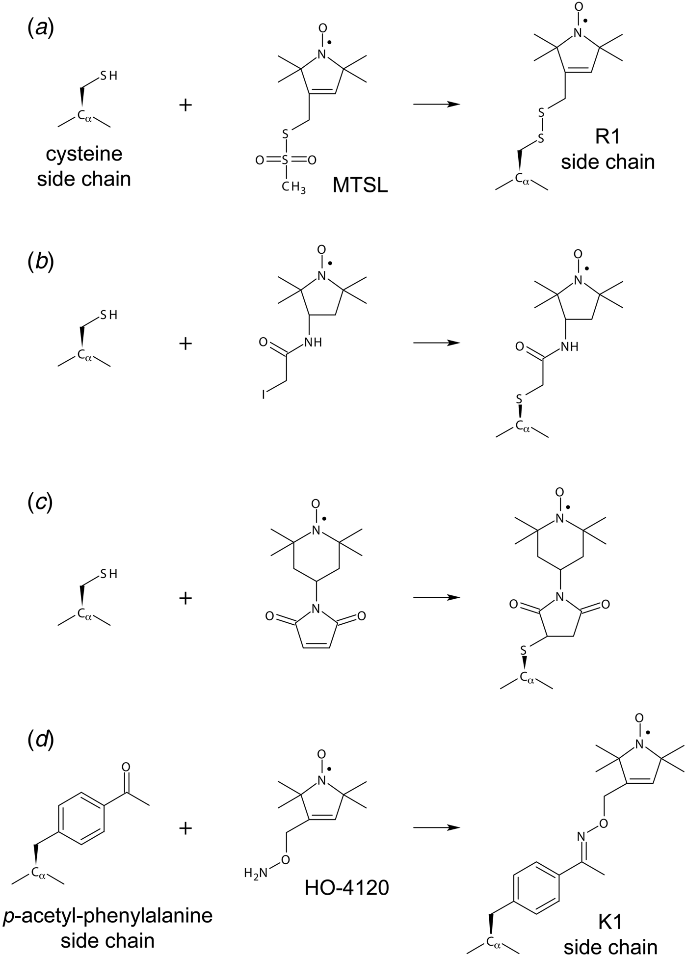
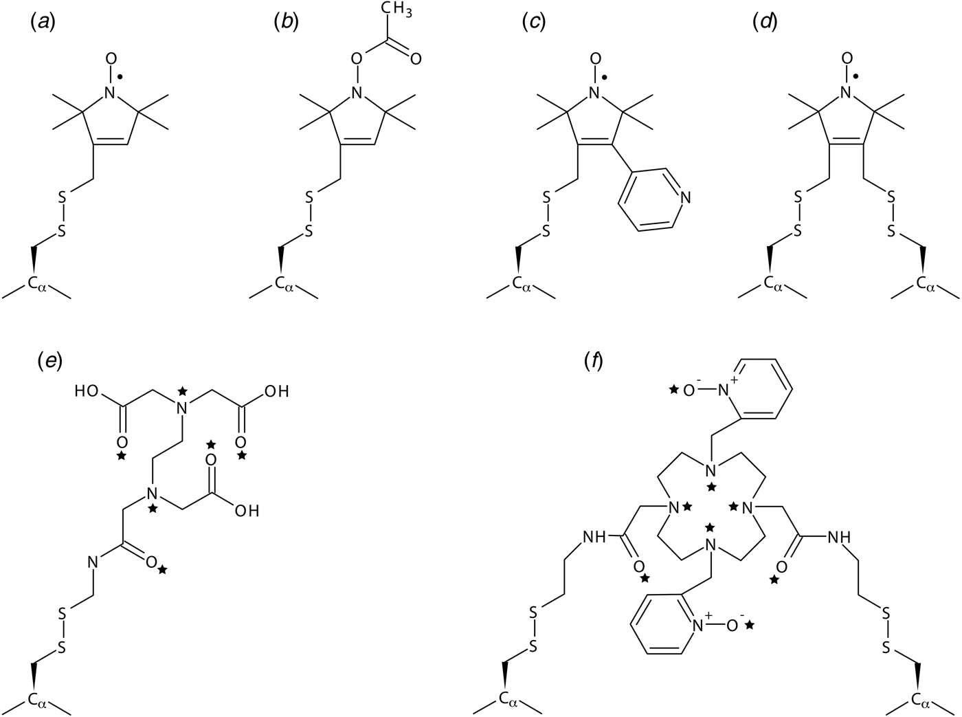
The use of paramagnetic restraints in biomolecular NMR was previously restricted primarily to metalloproteins, where a paramagnetic cation can easily replace the natural metal ligand (Bertini et al. Reference Bertini, Luchinat and Piccioli2001b; Cheng & Markley, Reference Cheng and Markley1995; Ubbink et al. Reference Ubbink, Worrall, Canters, Groenen and Huber2002). Although the underlying theory of PRE was originally developed in the 1950s (Bloembergen & Morgan, Reference Bloembergen and Morgan1961; Solomon, Reference Solomon1955) and the utility of PRE restraints for macromolecular structure determination was demonstrated in the 1980s (Kosen et al. Reference Kosen, Scheek, Naderi, Basus, Manogaran, Schmidt, Oppenheimer and Kuntz1986; Schmidt & Kuntz, Reference Schmidt and Kuntz1984), only recently have PRE measurements become practically useful and commonly performed due to the development of straightforward biochemical methods for site-specific introduction of paramagnetic labels in proteins (Battiste & Wagner, Reference Battiste and Wagner2000; Donaldson et al. Reference Donaldson, Skrynnikov, Choy, Muhandiram, Sarkar, Forman-Kay and Kay2001; Gaponenko et al. Reference Gaponenko, Howarth, Columbus, Gasmi-Seabrook, Yuan, Hubbell and Rosevear2000). A wide range of chemistries are available for conjugating a paramagnetic tag (either a nitroxide or a metal ion-bound chelator) to a protein (Hubbell et al. Reference Hubbell, Lopez, Altenbach and Yang2013; Jeschke, Reference Jeschke2013; Keizers & Ubbink, Reference Keizers and Ubbink2011); most common are those that involve a nitroxide group or a paramagnetic metal ion chelated by EDTA and are conjugated to the protein via an exposed cysteine (Kosen, Reference Kosen1989). The inherent flexibility of these tags was previously a hurdle for the quantitative analysis of PRE data, although these issues have largely been overcome through improved computational methods (Iwahara et al. Reference Iwahara, Schwieters and Clore2004b). More rigid tags have also been developed (Fawzi et al. Reference Fawzi, Fleissner, Anthis, Kalai, Hideg, Hubbell and Clore2011a; Keizers et al. Reference Keizers, Desreux, Overhand and Ubbink2007), and the use of such rigid tags is essential for measuring PCSs. Although PRE values are also affected by internal motion, they do not, like PCSs, have an orientational dependence, thus simplifying analysis and enabling the use of tags with flexible linkers.
The PRE is measured by taking the difference in relaxation rate between a paramagnetic state and a control diamagnetic state. PRE can be measured as either an enhancement of the longitudinal (Γ1) or transverse (Γ2) relaxation rate, although the measurement of Γ2 is advantageous (Clore & Iwahara, Reference Clore and Iwahara2009; Clore et al. Reference Clore, Tang and Iwahara2007) because its larger magnitude makes it a more sensitive probe and because it exhibits a simple dependence of the order parameter (S2) and is largely independent of the correlation time (τ i) of internal motion (Iwahara et al. Reference Iwahara, Schwieters and Clore2004b). Moreover, 1H transverse relaxation is a single-exponential process, whereas 1H longitudinal relaxation is multi-exponential due to cross-relaxation and, in the case of 1HN, water exchange, which results in perturbation of the observed 1H–Γ1 values. PRE values in a dynamic system cannot be directly interpreted as a single distance r, since both Γ1 and Γ2 depend upon the population-averaged value of 〈r −6〉. This difficulty with the quantitative analysis of PRE data has been addressed by the development of new theoretical and computational methods that use an ensemble approach to take into account the different conformations sampled by a paramagnetic label on the surface of a protein, calculating PRE order parameters on the fly from atomic coordinates as a simulation proceeds (Iwahara et al. Reference Iwahara, Schwieters and Clore2004b).
PRE data provide useful measurements of long distances in macromolecular structures (up to ~35 Å), and hundreds of individual distances can be measured from a single spin-label site (compared with FRET or DEER, where each doubly labeled sample only yields a single pairwise distance). As such, PRE data have been used to characterize the structures of a variety of macromolecules (Clore & Iwahara, Reference Clore and Iwahara2009), including soluble proteins (Battiste & Wagner, Reference Battiste and Wagner2000; Donaldson et al. Reference Donaldson, Skrynnikov, Choy, Muhandiram, Sarkar, Forman-Kay and Kay2001; Dvoretsky et al. Reference Dvoretsky, Gaponenko and Rosevear2002; Gaponenko et al. Reference Gaponenko, Howarth, Columbus, Gasmi-Seabrook, Yuan, Hubbell and Rosevear2000), membrane proteins (Liang et al. Reference Liang, Bushweller and Tamm2006; Roosild et al. Reference Roosild, Greenwald, Vega, Castronovo, Riek and Choe2005), and proteins in complex with other proteins (Card et al. Reference Card, Erbel and Gardner2005; Gross et al. Reference Gross, Moerke, Von Der Haar, Lugovskoy, Sachs, Mccarthy and Wagner2003; Mahoney et al. Reference Mahoney, Rastogi, Cahill, Girvin and Almo2000; Mal et al. Reference Mal, Ikura and Kay2002; Rumpel et al. Reference Rumpel, Becker and Zweckstetter2008), nucleic acids (Iwahara et al. Reference Iwahara, Anderson, Murphy and Clore2003, Reference Iwahara, Schwieters and Clore2004b; Ramos & Varani, Reference Ramos and Varani1998; Ueda et al. Reference Ueda, Kato, Ogawa, Torizawa, Kuramitsu, Iwai, Terasawa and Shimada2004; Varani et al. Reference Varani, Gunderson, Mattaj, Kay, Neuhaus and Varani2000), and oligosaccharides (Jain et al. Reference Jain, Venot, Umemoto, Leffler and Prestegard2001; Johnson et al. Reference Johnson, Brun, Mackenzie, Withers and Mcintosh1999; Macnaughtan et al. Reference Macnaughtan, Kamar, Alvarez-Manilla, Venot, Glushka, Pierce and Prestegard2007). Long-distance PRE restraints do not have the same power to constrain a molecular structure as a series of short-distance NOE measurements between atoms near in three-dimensional (3D) space (but not linear sequence), but these long-distance measurements complement these NOE-based short-distance measurements, and they are particularly important in scenarios where measuring many short-range distances by NOEs is difficult (e.g. membrane proteins) (Gottstein et al. Reference Gottstein, Reckel, Dotsch and Guntert2012).
PRE has also found applications in solid-state NMR, where additional challenges have had to be overcome, but where successes have included the de novo calculation of the fold of the protein GB1 (Sengupta et al. Reference Sengupta, Nadaud, Helmus, Schwieters and Jaroniec2012). Owing to extremely rapid transverse relaxation rates in the solid state, it is technically difficult to measure Γ2, so Γ1 is generally measured, requiring a paramagnetic center that maximizes the Γ1/Γ2 ratio. Thus, while paramagnetic centers with a very slow electron relaxation times (large values of τ s; e.g. nitroxides), are unsuitable due to a small Γ1/Γ2 ratio, paramagnetic centers with a more intermediate value of τ s give a more favorable Γ1/Γ2 ratio and are more appropriate for PRE measurements in the solid state (Sengupta et al. Reference Sengupta, Nadaud and Jaroniec2013). The large magnitude of intermolecular PREs due to molecular packing is another concern that arises in the solid state and must be considered (Nadaud et al. Reference Nadaud, Sengupta, Helmus and Jaroniec2011). Beyond their utility for generating distance restraints, the paramagnetic groups can be used as doping agents to increase the signal-to-noise (S/N) ratio and decrease the total acquisition time needed for a solid-state NMR experiment (Wickramasinghe et al. Reference Wickramasinghe, Kotecha, Samoson, Past and Ishii2007).
2.1.3 PRE and sparsely populated states
PRE is uniquely able to characterize otherwise invisible sparsely populated states (Anthis & Clore, Reference Anthis and Clore2013; Anthis et al. Reference Anthis, Doucleff and Clore2011; Bashir et al. Reference Bashir, Volkov, Ullmann and Ubbink2009; Bertini et al. Reference Bertini, Luchinat, Nagulapalli, Parigi and Ravera2012b; Fawzi et al. Reference Fawzi, Doucleff, Suh and Clore2010a; Iwahara & Clore, Reference Iwahara and Clore2006a; Iwahara et al. Reference Iwahara, Schwieters and Clore2004a; Tang et al. Reference Tang, Iwahara and Clore2006, Reference Tang, Schwieters and Clore2007, Reference Tang, Louis, Aniana, Suh and Clore2008b; Volkov et al. Reference Volkov, Worrall, Holtzmann and Ubbink2006) if two criteria are met: (1) the minor state must undergo rapid exchange; and (2) the distance between the paramagnetic center and some of the nuclei being measured must be shorter in the minor state than in the major state (Clore, Reference Clore2008; Clore & Iwahara, Reference Clore and Iwahara2009; Clore et al. Reference Clore, Tang and Iwahara2007). This is possible because a nucleus in close proximity to a paramagnetic center will exhibit an extremely large PRE (>1000 s−1), and the contribution from the close-proximity state will dominate the overall PRE measured for that nucleus, even if it constitutes a minor percentage of the total population (Fig. 2).
Characterizing a sparsely populated state by PRE. If a major state (A) is in exchange with a minor state (B), the effect of the minor state can be amplified by PRE if two points (corresponding to the paramagnetic center and observed nucleus) are in closer proximity in the minor state than in the major state. (a) In this example, the protein is in exchange between an extended state (A, r = 40 Å) and a compact state (B, r = 8 Å). If a nitroxide spin label is attached to one point, the PRE measured for a proton at the other point would be virtually zero in state A (Γ2,A = 0·12 s−1), but very large in state B (Γ2,B = 1900 s−1) causing broadening of the observed NMR signal. PRE values were calculated assuming a correlation time of τ c = 10 ns (corresponding to a protein at room temperature with a molecular weight of ~20 kDa). Spectra were calculated by solving the McConnell equations (Eqs. (16)–(20) and (57)) in MATLAB, assuming R 2,dia = 10 s−1 in each state (the height of the spectrum for state B [green] has been magnified 107 times for the purposes of visualization). If states A and B are in fast exchange on the PRE timescale (in this example: k ex ≫ Γ2,A − Γ2,B = 1900 s−1; τ ex ≪ 500 μs), the apparent PRE will be the population-averaged PRE of the two states (Γ2app = 0·99 × 0·12 s−1 + 0·01 × 1900 s−1 = 19·12 s−1). Thus, even although state B comprises only 1% of the total population, Γ2app arises almost exclusively from this minor state. (b) If the exchange rate is slower, the apparent PRE measured for A will be less than the population-weighted averaged PRE. Shown in black are simulated spectra for the system undergoing exchange with a rate of k ex = 102, 103, or 104 s−1. The dashed blue spectrum corresponds to the paramagnetic spectrum of A alone, and the dashed red spectrum corresponds to the population-weighted averaged paramagnetic spectrum under very fast exchange conditions (106 s−1). (c) Apparent PRE plotted against k ex. The PRE increases from 0·12 s−1 for a system undergoing very slow exchange (the value for state A alone) to 19·12 s−1 for a system undergoing very fast exchange.
With respect to the first (kinetic) requirement, the exchange must be fast on the PRE timescale, the latter meaning that the minor state exchanges with the major state at a rate that is much greater than the difference in PRE rates between the two states (k ex ≫ Γ2minor − Γ2major). In practice, this generally requires a timescale of τ ex < 250 μs (k ex > 1000 s−1). With respect to the second (structural) requirement, a shorter distance in the minor state could arise from two molecules forming a transient complex in the minor state or a conformational change that brings two parts of a molecule closer together in the dark state. In such a system, the overall PRE observed is an 〈r −6〉 population-weighted average of the PREs for all conformations in exchange. Because the PRE can be extremely large at close distances, even a very small population can cause a PRE to be much greater than the very small near-zero value that would be observed for a nucleus located far from a paramagnetic center. Under these circumstances, one can not only detect, but also characterize, the structural details of any minor state(s) giving rise to PREs, even those with populations of <1%. In fact, PREs are the most robust and comprehensive method for providing structural information on minor states. No other technique provides direct structural information on minor states, although others can provide some indirect information (through chemical shifts or RDCs) and can provide more kinetic information than PRE. A limitation, however, is that PRE data offer less insight into the kinetics of an exchange process, due to the difficulty of deconvoluting the contribution of different parameters (distance, exchange rate, and population) in systems undergoing exchange on the intermediate PRE timescale.
PRE studies have been used to gain insight into the transient states underlying a range of biomolecular processes, including protein/DNA interactions, protein/protein interactions, and interdomain interactions within proteins. For example, PRE data have revealed that the A-box of HMGB-1 interacts non-specifically with DNA, relevant to its role as a DNA-bending protein (Iwahara et al. Reference Iwahara, Schwieters and Clore2004a). PRE studies have characterized the inter-DNA-strand and intra-DNA-strand (‘sliding’) translocation of the transcription factors HoxD9 (Iwahara & Clore, Reference Iwahara and Clore2006a; Iwahara et al. Reference Iwahara, Zweckstetter and Clore2006), Oct1 (Takayama & Clore, Reference Takayama and Clore2011, Reference Takayama and Clore2012), and Sox2 (Takayama & Clore, Reference Takayama and Clore2012), revealing transient interactions with non-specific DNA sequences that facilitate the formation of the specific complex. The molecular details of the encounter complex between Enzyme I (EI) and the histidine-containing phosphocarrier protein (HPr), which plays a central role in the bacterial phosphotransferase system, have been elucidated (Fawzi et al. Reference Fawzi, Doucleff, Suh and Clore2010a; Tang et al. Reference Tang, Iwahara and Clore2006). PRE measurements have also demonstrated that cytochrome c and cytochrome c peroxidase form an encounter complex that samples conformational space near, although not identical to, the major species observed by X-ray crystallography, offering fundamental insight into the structural basis of electron transport (Volkov et al. Reference Volkov, Worrall, Holtzmann and Ubbink2006, Reference Volkov, Ubbink and Van Nuland2010). PRE studies have demonstrated that in the absence of a sugar ligand, maltose-binding protein (MBP) samples a partially closed state ~5% of the time that is similar – although not identical – to its closed sugar-bound state (Tang et al. Reference Tang, Schwieters and Clore2007) and in the absence of a peptide target, the calcium-sensing protein calmodulin (CaM) adopts a wide range of conformations, including structures similar in conformation to the more rigid peptide-bound complex (Anthis et al. Reference Anthis, Doucleff and Clore2011). These studies have offered a novel view into otherwise invisible states, providing fundamental insights into the process of molecular recognition and the complementary roles of conformational selection and induced fit.
2.2 Relaxation dispersion
2.2.1 Chemical exchange
If a molecule is in exchange between two states:
 $$A {\mathop{\rightleftharpoons}_{k_{{\rm BA}}}^{k_{{\rm AB}}}} B,$$
then the number of NMR peaks (as well as their height and linewidth) observed for a given nucleus will depend on the chemical shift difference (Δω) between the two states and on the exchange rate constant (k ex = k AB + k BA; the kinetics of exchange can also be described by the exchange lifetime, defined by τ ex = 1/k ex.) (Fig. 1). If Δω (given in angular frequency (rad·s−1), related to Δν (Hz) by Δω = 2πΔν) is much (>10 times) larger than k ex (the slow chemical shift exchange regime), two distinct peaks will be observed for the resonance, at the chemical shifts of the individual states, with peak volumes proportional to the populations of the individual states. If k ex is instead much (>10×) larger than Δω, a single peak will be observed at the population-weighted mean chemical shift; this is the fast chemical shift exchange regime. In the intermediate chemical shift exchange regime, however, the ratio of k ex/Δω takes a value close to 1 (±one order of magnitude), and line broadening is observed due to an increase in the observed transverse relaxation rate (R 2obs), which is the sum of the intrinsic transverse relaxation rate (R 20) and an exchange contribution (R ex) that depends upon k ex and Δω (Palmer & Massi, Reference Palmer and Massi2006; Palmer et al. Reference Palmer, Kroenke and Loria2001, Reference Palmer, Grey and Wang2005):
 $$R_2^{{\rm obs}} = R_2^{\rm 0} + R_{{\rm ex}}. $$
The value of R ex becomes insignificant in the extreme limits of the fast and slow exchange regimes. For certain conditions, simple expressions of R ex can be constructed for systems undergoing two-state exchange. In the slow exchange regime (k ex ≪ Δω), R ex is given by (Palmer et al. Reference Palmer, Kroenke and Loria2001):
 $$R_{{\rm ex,A}} = k_{{\rm AB}} = (1 - p_{\rm A} )k_{{\rm ex}} = p_{\rm B} k_{{\rm ex}}, $$
 $$R_{{\rm ex,B}} = k_{{\rm BA}} = (1 - p_{\rm B} )k_{{\rm ex}} = p_{\rm A} k_{{\rm ex}}, $$
where R ex,A is R ex measured for state A, R ex,B is R ex measured for state B, p A the population of state A (the observed state), and p B = 1 − p A the population of state B (the state in exchange with state A). There are two different values of R ex in the slow exchange regime because a separate peak is seen for each state. In the fast exchange regime (k ex ≫ Δω), R ex is given by (Palmer et al. Reference Palmer, Kroenke and Loria2001):
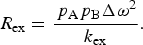 $$R_{{\rm ex}} = \displaystyle{{\,p_{\rm A} p_{\rm B} {\rm \Delta} \omega ^2} \over {k_{{\rm ex}}}}. $$
Thus, while R ex is independent of magnetic field strength (B 0) in the slow exchange regime, R ex depends on the square of the magnetic field strength (i.e. Δω 2) in the fast exchange regime.
If the population of the minor state is very small (p A ≫ p B), the following holds for all timescales (Swift & Connick, Reference Swift and Connick1962):
 $$R_{{\rm ex}} = \displaystyle{{\,p_{\rm A} p_{\rm B} k_{{\rm ex}}} \over {{\rm 1 + (}k_{{\rm ex}} /{\rm \Delta} \omega {\rm )}^2}} = \displaystyle{{\,p_{\rm A} p_{\rm B} k_{{\rm ex}} {\rm \Delta} \omega ^2} \over {{\rm \Delta} \omega ^2 + k_{{\rm ex}}^2}}. $$
Under these conditions, the exchange-induced chemical shift (ω ex) of state A – which is the difference in position of the peak in the exchanging system compared with its position in the absence of exchange – is given by:
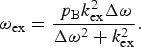 $$\omega _{{\rm ex}} = \displaystyle{{\,p_{\rm B} k_{{\rm ex}}^2 {\rm \Delta} \omega} \over {{\rm \Delta} \omega ^2 + k_{{\rm ex}}^2}}. $$
If states A and B have different intrinsic transverse relaxation rates (ΔR 20 = R 2,B0 − R 2,A0 > 0), then, for the case where p A ≫ p B, R ex is given by (Skrynnikov et al. Reference Skrynnikov, Dahlquist and Kay2002):
 $$R_{{\rm ex}} = k_{{\rm AB}} \displaystyle{{{\rm \Delta} R_2^0 \left( {k_{{\rm BA}} + {\rm \Delta} R_2^0} \right) + {\rm \Delta} \omega ^2} \over {\left( {k_{{\rm BA}} + {\rm \Delta} R_2^0} \right)^2 + {\rm \Delta} \omega ^2}}. $$
Under these same conditions, the exchange-induced chemical shift is (Skrynnikov et al. Reference Skrynnikov, Dahlquist and Kay2002):
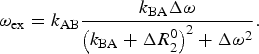 $$\omega _{{\rm ex}} = k_{{\rm AB}} \displaystyle{{k_{{\rm BA}} {\rm \Delta} \omega} \over {\left( {k_{{\rm BA}} + {\rm \Delta} R_2^0} \right)^2 + {\rm \Delta} \omega ^2}}. $$
For a complete description of an exchanging system, it is necessary to invoke the McConnell equations (McConnell, Reference Mcconnell1958), a modified form of the Bloch equations (Bloch, Reference Bloch1946) extended to incorporate chemical exchange. Transverse relaxation in an exchanging system can be described by the following matrix equation:
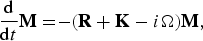 $$\displaystyle{{\rm d} \over {{\rm d}t}}{\bf M =} {\rm - (}{\bf R + K}-i{\bf \Omega} {\rm )}{\bf M}{\rm,} $$
where M is the vector describing the transverse magnetization of each state, R the matrix describing the transverse relaxation rates of each state, K the matrix describing the kinetic rates of exchange between each state, and Ω the matrix describing the chemical shift of each state. For a system undergoing two-site exchange between states A and B, these are given by:
 $${\bf M =} \left[ {\matrix{ {M_{\rm A}^ +} \cr {M_{\rm B}^ +} \cr}} \right],$$
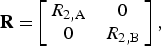 $${\bf R =} \left[ {\matrix{ {R_{2,{\rm A}}} & 0 \cr 0 & {R_{2,{\rm B}}} \cr}} \right],$$
 $${\bf K =} \left[ {\matrix{ {k_{{\rm AB}}} & { - k_{{\rm BA}}} \cr { - k_{{\rm AB}}} & {k_{{\rm BA}}} \cr}} \right],$$
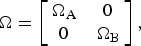 $${\bf \Omega} = \left[ {\matrix{ {{\rm \Omega} _{\rm A}} & 0 \cr 0 & {{\rm \Omega} _{\rm B}} \cr}} \right],$$
where M + is the transverse magnetization of each state (represented by a complex variable Mx + iMy) and Ω/2π is the chemical shift of each state. The McConnell equations can be solved (analytically for simple two-state cases (Palmer et al. Reference Palmer, Kroenke and Loria2001) or numerically for all cases by integration or by calculating the matrix exponential) to provide a time course of the magnetization (i.e. free induction decay):
 $${\bf M}{\rm (}t{\rm )} = {\bf A}\;{\rm \times}\; {\bf M}{\rm (0),}$$
where M(t) is the transverse magnetization vector M at time t, M(0) is the initial value of M at t = 0, and A(t) is a matrix of time-dependent elements determined by solving the McConnell equations. Fourier transformation of Eq. (21) yields a frequency-domain NMR spectrum, from which apparent relaxation rates can be extracted by line shape fitting.
2.2.2 CPMG and rotating frame relaxation dispersion
Even a very small population of an otherwise invisible second state (as long as p b ≥ 0.5%) can cause significant broadening of NMR peaks under conditions of intermediate exchange (in general τ ex ~100 μs–10 ms), allowing characterization by relaxation dispersion NMR and insight into the otherwise invisible minor state (Baldwin & Kay, Reference Baldwin and Kay2009; Korzhnev & Kay, Reference Korzhnev and Kay2008; Loria et al. Reference Loria, Berlow and Watt2008; Mittermaier & Kay, Reference Mittermaier and Kay2009; Neudecker et al. Reference Neudecker, Lundstrom and Kay2009; Palmer et al. Reference Palmer, Kroenke and Loria2001), using CPMG or R 1ρ experiments. These experiments are performed by measuring the apparent R 2obs of a nucleus (usually 15N or 13C, but also 1H) while varying the repetition rate of 180° pulses (CPMG) or the strength of a spin lock field (R 1ρ) to attenuate the contribution of R ex to the overall measured R 2 rate (Palmer et al. Reference Palmer, Grey and Wang2005).
In a CPMG relaxation dispersion experiment (Fig. 3), the effective observed R 2 (R 2,CPobs) is measured as a function of the CPMG field (ν CP [Hz]), which is the frequency of repetition pairs of 180° CPMG pulses and is related to τ CP [s], the delay between 180° CPMG pulses, by:
 $$\nu _{{\rm CP}} = \displaystyle{1 \over {2\tau _{{\rm CP}}}}. $$
Characterizing exchange with a ‘dark’ state by CPMG relaxation dispersion. Relaxation dispersion curves were simulated in MATLAB, showing the apparent observed transverse relaxation rate (R 2obs) as a function of the repetition rate of 180° CPMG pulses (ν CPMG, 0–1 kHz). Curves were calculated by solving the McConnell equations in MATLAB using Eq. (31). Curves are shown for range of exchange rates (k ex = 102–104 s−1) for a system where a visible species (p A = 95%) is in exchange with a dark state (p B = 5%), analogous to a 15N resonance with a chemical shift difference between states A and B of Δδ = 2 ppm. The blue curves correspond to a static B 0 field strength of 600 MHz (Δω/2π = 120 Hz), and the red curves correspond to 900 MHz (Δω/2π = 180 Hz). At a large ν CPMG, R 2obs approaches the intrinsic transverse relaxation rate R 20 (set here for both states to 10 s−1 at 600 MHz and 13 s−1 at 900 MHz). CPMG relaxation dispersion is most useful for characterizing exchange with a minor species when R ex (= R 2obs[ν CPMG = 0] − R 2obs[ν CPMG → ∞]) is largest, which occurs when k ex = Δω (~1000 s−1, middle panel).
At each CPMG field, the observed R 2 is given by:
 $$R_{2,{\rm CP}}^{{\rm obs}} = R_2^0 + R_{{\rm ex,CP}}, $$
where R 20 is the intrinsic transverse relaxation rate in the absence of exchange and R ex,CP is the contribution to transverse relaxation from chemical exchange broadening, which has been attenuated to some degree by CPMG pulses.
The parameters of interest are determined by fitting the CPMG data to a series of equations. Although the equations describing complicated systems involving three or more states can only be solved numerically, a system undergoing two-state exchange can be solved analytically (Carver & Richards, Reference Carver and Richards1972; Davis et al. Reference Davis, Perlman and London1994; Jen, Reference Jen1978; Palmer et al. Reference Palmer, Kroenke and Loria2001; Rule & Hitchens, Reference Rule and Hitchens2006):
 $$R_{2,{\rm CP}}^{{\rm obs}} = \displaystyle{1 \over 2}\left( {R_{2,{\rm A}}^0 + R_{2,{\rm B}}^0 + k_{{\rm ex}} - [2\nu _{{\rm CP}} ]\,\,\cosh ^{ - 1} \left[ {D_ + \cosh \,(\eta _ + ) - D_ - \cos \,(\eta _ - )} \right]} \right),$$
where
 $$D_{\rm \pm} = \displaystyle{1 \over 2}\left( {{\rm \pm} 1 + \displaystyle{{\psi + 2{\rm \Delta} \omega ^2} \over {[\psi ^2 + \zeta ^2 ]^{1/2}}}} \right),$$
 $$\eta _{\rm \pm} = \displaystyle{1 \over {\left( {2\nu _{{\rm CP}}} \right)\sqrt 2}} \left( {{\rm \pm} \psi + \left[ {\psi ^2 + \zeta ^2} \right]^{1/2}} \right)^{1/2}, $$
 $$\psi = \left( {R_{2,{\rm A}}^0 - R_{2,{\rm B}}^0 - p_{\rm A} k_{{\rm ex}} + p_{\rm B} k_{{\rm ex}}} \right)^2 - {\rm \Delta} \omega ^2 + 4p_{\rm A} p_{\rm B} k_{{\rm ex}}^2, $$
 $$\zeta = 2{\rm \Delta} \omega \left( {R_{2,{\rm A}}^0 - R_{2,{\rm B}}^0 - p_{\rm A} k_{{\rm ex}} + p_{\rm B} k_{{\rm ex}}} \right),$$
and where R 2,A0 is the R 2 of state A in the absence of chemical exchange (i.e. ν CP = ∞), R 2,B0 is the R 2 of state B in the absence of chemical exchange, p A is the population of state A, p B is the population of state B, and Δω is the difference in chemical shift between states A and B.
Simplified expressions can be written for R 2,CPobs under certain scenarios. In the fast exchange regime, the expression for R 2,CPobs can be simplified to (Palmer et al. Reference Palmer, Kroenke and Loria2001):
 $$R_{2,{\rm CP}}^{{\rm obs}} = p_{\rm A} R_{2,{\rm A}}^0 + p_{\rm B} R_{2,{\rm B}}^0 + \left( {\displaystyle{{\,p_{\rm A} p_{\rm B} {\rm \Delta} \omega ^2} \over {k_{{\rm ex}}}}} \right)\left( {1 - \displaystyle{{2[2\nu _{{\rm CP}} ]} \over {k_{{\rm ex}}}} \tanh \left[ {\displaystyle{{k_{{\rm ex}}} \over {2\left( {2\nu _{{\rm CP}}} \right)}}} \right]} \right).$$
If p A ≫ p B, regardless of the timescale, the expression for R 2obs can be simplified to (Ishima & Torchia, Reference Ishima and Torchia1999):
 $$R_{2,{\rm CP}}^{{\rm obs}} = R_2^0 + \displaystyle{{\,p_{\rm A} p_{\rm B} {\rm \Delta} \omega ^2 k_{{\rm ex}}} \over {k_{{\rm ex}}^2 + \left( {\,p_{\rm A}^2 {\rm \Delta} \omega ^4 + 48\left[ {2\nu _{{\rm CP}}} \right]^4} \right)^{1/2}}}, $$
where R 20 is equal to R 2,A0 in the slow exchange regime and p AR 2,A0 + p BR 2,B0 in the fast exchange regime.
For systems more complex than a two-state system, R 2obs is not given by an analytical expression, but can only be calculated by numerical solution of the McConnell equations. For any system, the transverse magnetization at the end of a CPMG period (T CP) consisting of an even number (2n) of 180° pulses, each separated by time τ CP, is given by (Palmer et al. Reference Palmer, Kroenke and Loria2001):
 $${\bf M}{\rm (2}n\tau _{{\rm CP}} ) = \left( {{\bf AA}^* {\bf A}^* {\bf A}} \right)^n \;{\bf M}{\rm (0),}$$
where M(2nτ CP) is the transverse magnetization vector at time T CP = 2nτ CP and A* is the complex conjugate of A (Eq. (21)) when the McConnell equations have been solved for t = τ CP/2 (Palmer et al. Reference Palmer, Kroenke and Loria2001).
The CPMG relaxation dispersion curve has a complex shape that is a function of k ex, the populations of the states undergoing exchange, and the chemical shift difference between these states. If the system is in exchange between two states, a simple model can be used to fit the data; more complicated multi-state models can then be employed if the two-site fit is not adequate, although one is generally limited to three-site exchange models to improve the fit without overfitting the data (Korzhnev & Kay, Reference Korzhnev and Kay2008; Li et al. Reference Li, Martins and Rosen2011; Mittermaier & Kay, Reference Mittermaier and Kay2009; Neudecker et al. Reference Neudecker, Lundstrom and Kay2009; Trott & Palmer, Reference Trott and Palmer2004). The contribution of the populations and chemical shift differences to R ex cannot be separated a priori for data recorded at a single magnetic field. Thus, unless the populations or chemical shift differences are already known, one must record data at different B 0 magnetic field strengths, because the populations of the species are independent of the magnetic field, while the differences in frequency are linearly proportional to the magnetic field.
A system in intermediate chemical exchange can also be characterized by rotating frame R 1ρ relaxation dispersion, fitting the effective R 1ρ ( = 1/T 1ρ) as a function of the effective spin-lock field strength (ω e). The observed R 1ρ for a given spin-lock field (R 1ρobs) is given by the sum of R 1ρ in the absence of exchange (R 1ρ0) plus the contribution to R 1ρ from chemical exchange broadening (R ex,1ρ), which has been attenuated to some degree by the spin-lock field:
 $$R_{1\rho} ^{{\rm obs}} = R_{1\rho} ^{\rm 0} + R_{{\rm ex,1}\rho}. $$
For two-state exchange in the fast exchange regime, the expression for R 1ρobs is given by (Davis et al. Reference Davis, Perlman and London1994; Deverell et al. Reference Deverell, Morgan and Strange1970; Meiboom, Reference Meiboom1961; Palmer et al. Reference Palmer, Kroenke and Loria2001; Rule & Hitchens, Reference Rule and Hitchens2006):
 $$R_{1\rho} ^{{\rm obs}} = R_{1\rho} ^0 + \displaystyle{{\,p_{\rm A} p_{\rm B} {\rm \Delta} \omega ^2 k_{{\rm ex}}} \over {k_{{\rm ex}}^2 + \omega _{\rm e}^2}} \sin ^2 \theta, $$
where R 1ρ0 is R 1ρ in the absence of chemical exchange (i.e. ω e = ∞) and the angle between the B 1 spin-lock field and the static B 0 field is given by:
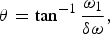 $$\theta = \tan ^{ - 1} \displaystyle{{\omega _1} \over {\delta \omega}}, $$
where ω 1 (rad·s−1) is the strength of the spin-lock field and δω (rad·s−1) is the frequency offset (the difference between the resonance frequency of the nucleus and the transmitter frequency). The effective spin-lock field strength is given by:
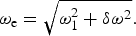 $$\omega _{\rm e} = \sqrt {\omega _1^2 + \delta \omega ^2}. $$
If p A ≫ p B and the spin-lock field is on resonance (δω = 0), R 1ρobs can be expressed regardless of the timescale as (Meiboom, Reference Meiboom1961):
 $$R_{1\rho} ^{{\rm obs}} = R_{1\rho} ^0 + \displaystyle{{\,p_{\rm A}^2 p_{\rm B} {\rm \Delta} \omega ^2 k_{{\rm ex}}} \over {k_{{\rm ex}}^2 + p_{\rm A}^2 {\rm \Delta} \omega ^2 + \omega _1^2}}, $$
where R 1ρ in the absence of chemical exchange in the slow exchange regime is given by:
 $$R_{1\rho} ^{\rm 0} = R_{1,{\rm A}}^0 \cos ^2 \theta + R_{2,{\rm A}}^0 \sin ^2 \theta $$
and in the fast exchange regime is given by:
 $$R_{1\rho} ^0 = \left( {\,p_{\rm A} R_{1,{\rm A}}^0 + p_{\rm B} R_{1,{\rm B}}^0} \right)\cos ^2 \theta + \left( {\,p_{\rm A} R_{2,{\rm A}}^0 + p_{\rm B} R_{2,{\rm B}}^0} \right)\sin ^2 \theta. $$
For off-resonance spin-lock fields, as long as the population of the minor state is very small (p A ≫ p B), R 1ρobs can be expressed in a form analogous to Eq. (30) (Palmer, Reference Palmer2014):
 $$R_{1\rho} ^{{\rm obs}} = R_{1\rho} ^{\rm 0} + \displaystyle{{\,p_{\rm A} p_{\rm B} {\rm \Delta} \omega ^2 k_{{\rm ex}}} \over {k_{{\rm ex}}^2 + \omega _{{\rm e,A}}^2 \omega _{{\rm e,B}}^2 /\omega _{{\rm e,ave}}^2}}, $$
where ω e,A is the effective spin-lock field (Eq. (35)) for the chemical shift of state A, ω e,B for state B, and ω e,ave is the effective spin-lock field for the population-averaged chemical shift of states A + B. If the intrinsic transverse relaxation rates differ between the two states (ΔR 20 = R 2,A − R 2,B > 0), R 1ρobs can be given by the following expression, which is accurate as long as p A ≫ p B (Palmer, Reference Palmer2014):
 $$R_{1\rho} ^{{\rm obs}} = R_{1\rho} ^{\rm 0} + k_{{\rm AB}} \displaystyle{{k_{{\rm BA}} \left( {{\rm \Delta} \omega ^2 + \left[ {{\rm \Delta} R_2^0} \right]^2} \right) + {\rm \Delta} R_2^0 \left( {\omega _{{\rm e,A}}^2 + k_{{\rm BA}}^2} \right)} \over {k_{{\rm BA}} \left( {{\rm \Delta} \omega _{{\rm e,B}}^2 + k_{{\rm BA}}^2 + \left[ {{\rm \Delta} R_2^0} \right]^2} \right) + {\rm \Delta} R_2^0 \omega _1^2}}. $$
A more comprehensive analytical expression is given by Baldwin & Kay (Reference Baldwin and Kay2013). Under all circumstances, though, values of R 1ρobs can be calculated by solving the McConnell equations using the same matrices as for a saturation transfer experiment (cf. Eqs. (82)–(84) below).
An advantage of R 1ρ experiments is that they can characterize faster exchange processes than CPMG experiments. Whereas CPMG data alone can be used to characterize exchange on a timescale of roughly ~500 μs–5 ms, R 1ρ relaxation dispersion experiments can measure exchange processes as fast as k ex < 40 000 s−1 (τ ex > 25 μs) (Ban et al. Reference Ban, Gossert, Giller, Becker, Griesinger and Lee2012; Hansen et al. Reference Hansen, Nikolova, Casiano-Negroni and Al-Hashimi2009; Lundstrom & Akke, Reference Lundstrom and Akke2005; Weininger et al. Reference Weininger, Blissing, Hennig, Ahlner, Liu, Vogel, Akke and Lundstrom2013). The remainder of this section, however, focuses on CPMG relaxation dispersion.
2.2.3 Practical aspects of CPMG
From a series of CPMG experiments, one can determine the populations of the major and minor states, the rate of exchange between the states, and the magnitude of the chemical shift difference between the states, which offers indirect structural insight into the minor state. However, CPMG data alone only directly provide information on the magnitude, but not direction, of chemical shift differences. The direction of the chemical shift differences can be determined by either comparing the chemical shift of the resonance between heteronuclear single (HSQC) and multiple (HMQC) quantum coherence spectra or between spectra acquired at different B 0 fields (Bouvignies et al. Reference Bouvignies, Korzhnev, Neudecker, Hansen, Cordes and Kay2010; Skrynnikov et al. Reference Skrynnikov, Dahlquist and Kay2002). As Δω is directly proportional to B 0, moving from a lower to a higher B 0 field has the effect of decreasing k ex/Δω, thus slowing the exchange regime and moving the frequency of the resonance closer to its intrinsic chemical shift (slow exchange) and farther from the population-averaged chemical shift (fast exchange). The difference in chemical shift observed between HSQC and HMQC spectra arises from the fact that, for 15N for example, the exchange regime in the HSQC experiment is characterized by k ex/Δω N, but in the HMQC, exchange of zero-quantum and double-quantum magnetization are characterized by k ex/(Δω N − Δω H) and k ex/(Δω N + Δω H), respectively, which do not average linearly, thus altering the exchange regime and giving rise to a small difference in chemical shift between the HSQC and HMQC spectra (Skrynnikov et al. Reference Skrynnikov, Dahlquist and Kay2002). Likewise, if there is any direct knowledge of the chemical shift of the minor state from other measurements (e.g. ligand-binding studies, protein-folding/unfolding studies, concentration dependence, etc.), such information on the magnitude of chemical shift change can assist the CPMG fitting process.
The fitting of CPMG data is prone to difficulties, and distinguishing between k ex, Δω, and p B requires resonances undergoing exchange in the intermediate regime, with at least some satisfying the condition k ex/Δω < 2; this limits the range of k ex values measurable from CPMG alone to between ~200 and ~2000 s−1. However, the incorporation of additional chemical shift information (e.g. from HSQC versus HMQC spectra) can extend this range further into the fast timescale, allowing fitting of data in the fast-intermediate exchange regime, up to k ex/Δω ~ 4 (in practice, exchange rates up to k ex ~ 6000 s−1; τ ex ~ 170 μs) (Vallurupalli et al. Reference Vallurupalli, Bouvignies and Kay2011). The study of fast exchange processes by CPMG relaxation dispersion can be problematic in general, leading to large errors when the repetition rate (ν CP = 1/τ CP) is not much greater than k ex. However, it has been demonstrated that if this condition is not satisfied, these errors can be reduced dramatically (from ~50 to ~5%) by measuring the intrinsic relaxation rate R 20 using an R 1ρ experiment with a high spin-lock field (Ban et al. Reference Ban, Mazur, Carneiro, Sabo, Giller, Koharudin, Becker, Gronenborn, Griesinger and Lee2013).
Relaxation dispersion experiments on proteins are most commonly performed on the backbone 15N nucleus, although measurements on 1HN, 13Cα, 1Hα, 13Cβ, and 13C′ backbone nuclei and side chain methyl 1H and 13C nuclei (Hansen et al. Reference Hansen, Vallurupalli, Lundstrom, Neudecker and Kay2008b; Ishima & Torchia, Reference Ishima and Torchia2003; Lundstrom et al. Reference Lundstrom, Vallurupalli, Religa, Dahlquist and Kay2007, Reference Lundstrom, Hansen, Vallurupalli and Kay2009a, Reference Lundstrom, Lin and Kay2009b) are also feasible. Minor state chemical shifts derived from CPMG studies can be used to calculate backbone torsion angle restraints for the minor state using a program such as TALOS-N (Shen & Bax, Reference Shen and Bax2013), and it is possible to calculate the structure of a small protein from backbone chemical shifts alone, using programs such as CHESHIRE (Cavalli et al. Reference Cavalli, Salvatella, Dobson and Vendruscolo2007) or CS-Rosetta (Shen et al. Reference Shen, Lange, Delaglio, Rossi, Aramini, Liu, Eletsky, Wu, Singarapu, Lemak, Ignatchenko, Arrowsmith, Szyperski, Montelione, Baker and Bax2008, Reference Shen, Vernon, Baker and Bax2009), which rely upon matching the empirical chemical shifts with a peptide fragment database. Such an approach can provide direct insight into the structure of a minor state (Korzhnev et al. Reference Korzhnev, Religa, Banachewicz, Fersht and Kay2010), although complications can arise if the minor state is partially unfolded, as the databases used for calculation of structures from chemical shifts are derived from folded proteins. It has also been demonstrated that the orientation of bond vectors in minor states can be measured through relaxation dispersion experiments (Hansen et al. Reference Hansen, Vallurupalli and Kay2008a; Vallurupalli et al. Reference Vallurupalli, Hansen, Stollar, Meirovitch and Kay2007, Reference Vallurupalli, Hansen and Kay2008a, Reference Vallurupalli, Hansen and Kayb). By performing relaxation dispersion experiments in weakly aligned media, one can measure RDCs and residual chemical shift anisotropy (RCSA) for the minor state, although highly accurate measurements are required to detect the small effect of the minor state on these observables. Additionally, the introduction of a paramagnetic group with an anisotropic g-tensor will magnify Δω if different PCSs are observed between the different states, potentially causing additional exchange broadening and facilitating CPMG relaxation dispersion studies. This strategy has been applied to intrinsic metalloproteins (Wang et al. Reference Wang, Srisailam, Yee, Lemak, Arrowsmith, Prestegard and Tian2007) and to otherwise diamagnetic proteins by incorporating a rigid metal-chelating paramagnetic tag to induce relaxation dispersion when none was apparent in the diamagnetic state of the protein (Eichmuller & Skrynnikov, Reference Eichmuller and Skrynnikov2007; Hass et al. Reference Hass, Keizers, Blok, Hiruma and Ubbink2010).
For larger proteins, the favorable spectral properties of methyl groups make methyl 13C, 1H, and 2H (D) nuclei useful probes of dynamics (Igumenova et al. Reference Igumenova, Frederick and Wand2006; Ruschak & Kay, Reference Ruschak and Kay2010). Methods have been developed to express recombinant proteins in Escherichia coli with various methyl isotopic labeling schemes (Tugarinov et al. Reference Tugarinov, Kanelis and Kay2006). Favorable relaxation properties are seen in 13CDH2-labeled methyl groups, and, for 13CH3-labeled methyl groups on a perdeuterated background, acquiring data with an HMQC experiment instead of an HSQC experiment allows one to take advantage of the slower multiple quantum relaxation due to cancellation of dipolar interactions within the methyl group (i.e. the ‘methyl-TROSY’ effect), helping make large systems accessible to analysis by NMR (Tugarinov et al. Reference Tugarinov, Hwang, Ollerenshaw and Kay2003). Using these methods, 13C CPMG relaxation dispersion experiments have been performed to characterize intermediate dynamics in systems as large as the 82-kDa enzyme malate synthase G (Korzhnev et al. Reference Korzhnev, Kloiber, Kanelis, Tugarinov and Kay2004a), the 230-kDa HsIV component of the bacterial proteasome (Shi & Kay, Reference Shi and Kay2014), and the 670-kDa 20S core particle of the archaeal proteasome (Sprangers & Kay, Reference Sprangers and Kay2007). Using a labeling scheme that isolates 1H spins, 1H CPMG relaxation dispersion experiments can also be performed on methyl groups (Hansen et al. Reference Hansen, Lundstrom, Velyvis and Kay2012; Otten et al. Reference Otten, Villali, Kern and Mulder2010).
2.2.4 Applications of CPMG
CPMG relaxation dispersion is well suited for studying protein folding, due to its ability to identify minor states (i.e. folding intermediates) in exchange with a visible (folded or unfolded) species on an intermediate timescale (Fig. 3). These folding intermediates occupy local minima (i.e. ‘frustrations’) (Ferreiro et al. Reference Ferreiro, Cho, Komives and Wolynes2005) on an otherwise smooth, minimally frustrated protein-folding energy landscape (Bryngelson & Wolynes, Reference Bryngelson and Wolynes1987; Onuchic et al. Reference Onuchic, Lutheyschulten and Wolynes1997). CPMG relaxation dispersion studies on the folding of the SH3 domain from Fyn have identified an intermediate in the folding pathway (populated at ~1–2% at equilibrium), which has evaded detection by other methods and contains both native (central β-sheet) and non-native structural elements (Korzhnev et al. Reference Korzhnev, Salvatella, Vendruscolo, Di Nardo, Davidson, Dobson and Kay2004b, Reference Korzhnev, Neudecker, Zarrine-Afsar, Davidson and Kay2006; Neudecker et al. Reference Neudecker, Zarrine-Afsar, Davidson and Kay2007, Reference Neudecker, Lundstrom and Kay2009). Backbone 1H, 13C, and 15N chemical shifts and 1H–15N RDCs from CPMG relaxation dispersion were used to determine the structure, using CS-Rosetta, of an intermediate in the folding pathway of the FF domain from HYPA/FBP11, revealing a folding core comprising helices H1 and H2, and also other non-native interactions that slow the kinetics of folding (Korzhnev et al. Reference Korzhnev, Religa, Banachewicz, Fersht and Kay2010). A similar approach was used to solve the structure of a folding intermediate of a mutant of the Fyn SH3 domain, revealing an exposed β-strand that could potentially participate in protein misfolding and aggregation (Neudecker et al. Reference Neudecker, Robustelli, Cavalli, Walsh, Lundstrom, Zarrine-Afsar, Sharpe, Vendruscolo and Kay2012). The structure of a transient state of T4 lysozyme with an occluded binding cavity was also revealed in this manner (Bouvignies et al. Reference Bouvignies, Vallurupalli, Hansen, Correia, Lange, Bah, Vernon, Dahlquist, Baker and Kay2011). 15N CPMG relaxation dispersion data, in conjunction with chemical shift titrations, have been used to explore how an intrinsically unstructured peptide (pKID) undergoes folding upon binding to its target, the KIX domain of the CREB-binding protein (Sugase et al. Reference Sugase, Dyson and Wright2007); binding proceeds through an intermediate state consisting of partially folded pKID bound to KIX, consistent with an induced fit mechanism of binding (Wright & Dyson, Reference Wright and Dyson2009).
CPMG relaxation dispersion has proven to be a valuable tool for exploring the connection in enzymes between the catalytic rate and internal conformational dynamics (Villali & Kern, Reference Villali and Kern2010), an area that is the subject of a lively scientific debate (Kamerlin & Warshel, Reference Kamerlin and Warshel2010; Karplus, Reference Karplus2010; Pisliakov et al. Reference Pisliakov, Cao, Kamerlin and Warshel2009). Results from CPMG relaxation dispersion studies have demonstrated close correspondence between the k ex of conformational exchange and catalytic turnover (k cat) for a variety of enzymes, including HIV protease (Ishima et al. Reference Ishima, Freedberg, Wang, Louis and Torchia1999), RNase A (Cole & Loria, Reference Cole and Loria2002; Watt et al. Reference Watt, Shimada, Kovrigin and Loria2007), adenylate kinase (Adk) (Wolf-Watz et al. Reference Wolf-Watz, Thai, Henzler-Wildman, Hadjipavlou, Eisenmesser and Kern2004), cyclophilin A (Eisenmesser et al. Reference Eisenmesser, Millet, Labeikovsky, Korzhnev, Wolf-Watz, Bosco, Skalicky, Kay and Kern2005), dihydrofolate reductase (DHFR) (Boehr et al. Reference Boehr, Mcelheny, Dyson and Wright2006, Reference Boehr, Dyson and Wright2008, Reference Boehr, Mcelheny, Dyson and Wright2010), flavin oxidoreductase (Vallurupalli & Kay, Reference Vallurupalli and Kay2006), and triosphosphate isomerase (Kempf et al. Reference Kempf, Jung, Ragain, Sampson and Loria2007). DHFR undergoes exchange with a minor open conformation at a rate that is identical to product dissociation, which is the rate-limiting step in catalysis (Boehr et al. Reference Boehr, Mcelheny, Dyson and Wright2006); its hydride transfer step is also closely tied to the dynamics of conformational exchange (Boehr et al. Reference Boehr, Dyson and Wright2008). Likewise, it has been demonstrated by CPMG relaxation dispersion that the catalytic tunover (k cat) of Adk is limited by the rate of opening of the nucleotide-binding lid (Wolf-Watz et al. Reference Wolf-Watz, Thai, Henzler-Wildman, Hadjipavlou, Eisenmesser and Kern2004). Thus, for processes that occur on an intermediate timescale, relaxation dispersion offers exceptional insight into molecular dynamics, and in some cases into the structures of otherwise invisible minor states.
2.3 Saturation transfer
2.3.1 Principles and applications of saturation transfer
States that are invisible because they are sparsely populated or because they involve large, slowly tumbling molecules can be detected by saturation transfer if there are resonances in the minor state that can be saturated by off-resonance radiofrequency (RF) radiation that does not saturate the resonances of the major state; this saturation can then be transferred to the visible species by chemical exchange. Resonances can be selectively saturated in the dark state if their chemical shifts are sufficiently different from those in the visible state or if the dark state resonances are broadened considerably compared with those in the visible state. The DEST experiment can be used to characterize larger assemblies and aggregates that are invisible because they tumble slowly (causing large transverse relaxation rates and significant line broadening), as long as the large invisible state is in exchange with a smaller visible state on an intermediate-to-slow timescale (500 μs–1 s) (Fawzi et al. Reference Fawzi, Ying, Torchia and Clore2010b, Reference Fawzi, Ying, Ghirlando, Torchia and Clore2011b, Reference Fawzi, Ying, Torchia and Clore2012; Libich et al. Reference Libich, Fawzi, Ying and Clore2013). The CEST experiment, on the other hand, can be used to visualize a minor state in exchange with a major state, as long as the lifetime of the minor state is ~2–100 ms, its rotational correlation time is comparable to the major species, and it exhibits significantly different chemical shifts from the major state (Vallurupalli et al. Reference Vallurupalli, Bouvignies and Kay2012). Both experiments involve the application of off-resonance RF radiation to saturate a nucleus (usually 15N, but also 13C and 1H) in the minor state (Fig. 4).
Characterizing ‘dark’ states by exchange saturation transfer. Saturation profiles are plotted for (a) CEST and (b) DEST experiments by solving the homogeneous McConnell equations (Eqs. (82)–(84)) in MATLAB. The y-axis gives the ratio of the peak intensity measured in the presence of a CW RF B 1 field (I sat) over the peak intensity measured for a reference experiment in the absence of the saturation field (I ref). The x-axis gives the frequency offset of the applied B 1 field. Note that the units are (a) in Hz for the CEST profiles, but are (b) in kHz for the DEST profiles, where the x-axis has been expanded almost 50 fold to accommodate the broader DEST profiles. B 1 field strengths (applied in the x-dimension) are (a) 2·5 Hz (green), 5 Hz (cyan), 10 Hz (blue), and 25 Hz (purple) for CEST and (b) 25 Hz (green), 50 Hz (cyan), 100 Hz (blue), and 250 kHz (purple) for DEST (i.e. the DEST experiment is performed at about one order of magnitude higher B 1 field strength than CEST). In this figure, a major visible state A (p A = 95%) is separated from a minor dark state B (p B = 5%) by a chemical shift difference of Δω/2π = 120 Hz (e.g. 2 ppm for 15N in a 600 MHz spectrometer). For the CEST profiles (a), R 20 = 10 s−1 and R 1 = 1 s−1 for both states. For the DEST profiles (b), R 2,B0 = 10 000 s−1. CW saturation was applied for 1 s (= 1 × T 1). Results are shown for a system undergoing no exchange (top; i.e. the saturation profile of the major visible species A alone), and exchange at a rate of k ex = 1, 10, and 100 s−1 (bottom). Full saturation of the signal (I sat/I ref = 0) occurs when the B 1 field is applied on resonance to state A, and saturation can be transferred from states B to A by exchange either from (a) on-resonance saturation of state B due to a different chemical shift (CEST) or (b) off-resonance saturation of the broader profile of state B due to its faster rate of transverse relaxation (DEST).
A DEST or CEST experiment yields a plot of signal intensity versus the chemical shift offset of the B 1 saturating field for each resonance being monitored. These profiles can then be fit to a model (based on the McConnell equations (McConnell, Reference Mcconnell1958)) to determine the populations of and rates of exchange between each state. In addition to these kinetic and thermodynamic parameters, the DEST experiment also provides information on the transverse relaxation rates (R 2) of the resonances in the dark state (Fawzi et al. Reference Fawzi, Ying, Ghirlando, Torchia and Clore2011b, Reference Fawzi, Ying, Torchia and Clore2012). The CEST experiment provides direct information on the chemical shifts of the minor state (Bouvignies & Kay, Reference Bouvignies and Kay2012a, Reference Bouvignies and Kayb; Vallurupalli et al. Reference Vallurupalli, Bouvignies and Kay2012), which are difficult to extract from DEST data due to the broadness of the saturation transfer profiles (Fawzi et al. Reference Fawzi, Ying, Torchia and Clore2012).
NMR saturation transfer experiments were originally developed in the 1960s (Forsén & Hoffman, Reference Forsén and Hoffman1963), and the DEST and CEST experiments are related to small molecule saturation transfer difference (STD) NMR spectroscopy, where the broader resonances in a larger macromolecule are saturated, and saturation is transferred to a bound ligand via cross-relaxation and ultimately to the NMR-visible unbound ligand via chemical exchange (Mayer & Meyer, Reference Mayer and Meyer1999). Saturation transfer found some early biomolecular applications (Cayley et al. Reference Cayley, Albrand, Feeney, Roberts, Piper and Burgen1979; Gupta & Redfield, Reference Gupta and Redfield1970), although CEST was first employed in MRI, where exchangeable protons with a chemical shift distinct from water (either in endogenous molecules or introduced CEST contrast agents) are saturated, and this saturation is transferred to bulk water via slow chemical exchange, thus amplifying these otherwise invisible signals to provide additional contrast (Van Zijl & Yadav, Reference Van Zijl and Yadav2011; Ward et al. Reference Ward, Aletras and Balaban2000). More recently, PCSs from paramagnetic groups (chelated lanthanides) have been used to generate even larger chemical shifts in paraCEST imaging, enabling faster timescales for which k ex ≪ Δω remains true (Hancu et al. Reference Hancu, Dixon, Woods, Vinogradov, Sherry and Lenkinski2010; Vinogradov et al. Reference Vinogradov, Sherry and Lenkinski2013). Interestingly, one of the earliest biomolecular applications of saturation transfer involved using the hyperfine shifts in Fe3+-bound cytochrome c to study less-well-resolved Fe2+-bound cytochrome c via chemical exchange (Gupta & Redfield, Reference Gupta and Redfield1970). More recently, the applications of saturation transfer have been expanded to observe invisible states in macromolecules by CEST (Bouvignies & Kay, Reference Bouvignies and Kay2012a, Reference Bouvignies and Kayb; Vallurupalli et al. Reference Vallurupalli, Bouvignies and Kay2012) and DEST (Fawzi et al. Reference Fawzi, Ying, Ghirlando, Torchia and Clore2011b, Reference Fawzi, Ying, Torchia and Clore2012, Reference Fawzi, Libich, Ying, Tugarinov and Clore2014; Libich et al. Reference Libich, Fawzi, Ying and Clore2013).
2.3.2 The DEST experiment
The DEST experiment is used to characterize a visible species in exchange with a dark state that is invisible due to its large size (Fawzi et al. Reference Fawzi, Ying, Torchia and Clore2010b, Reference Fawzi, Ying, Ghirlando, Torchia and Clore2011b, Reference Fawzi, Ying, Torchia and Clore2012, Reference Fawzi, Libich, Ying, Tugarinov and Clore2014; Libich et al. Reference Libich, Fawzi, Ying and Clore2013). Owing to the rapid transverse relaxation rate of the signals in a slowly tumbling large dark state, these resonances can be saturated far off resonance at frequencies that do not excite the narrow signals of the rapidly tumbling visible species in the absence of the larger dark state. If the invisible species converts to the visible species at a rate that is of the order of or faster than its longitudinal relaxation rate, saturation will be transferred to the NMR-visible species and observed as a loss of intensity of cross-peaks for the visible species. Thus, it becomes possible to detect and characterize large aggregates and macromolecular assemblies that would otherwise be invisible. The DEST experiment is explored in greater detail in Section 3.
DEST is complementary to the transferred nuclear Overhauser effect (TRNOE) (Clore & Gronenborn, Reference Clore and Gronenborn1982, Reference Clore and Gronenborn1983), which offers structural restraints (in the form of short interproton distances) for a bound state in fast exchange with the free state. The TRNOE, however, is really only applicable in the case of exchanging systems involving small (low molecular weight) ligands that exhibit positive (or negligibly small) NOEs in the free state and large negative NOEs in the bound (high-molecular weight) state. DEST is qualitatively similar to other saturation-based experiments, including CEST and STD (Post, Reference Post2003). However, unlike STD, DEST offers quantitative results when performed on a heteronucleus (e.g. 15N and 13C), as it is not complicated by spin diffusion, which occurs in 1H saturation experiments (Bodner et al. Reference Bodner, Dobson and Bax2009; Fawzi et al. Reference Fawzi, Ying, Torchia and Clore2010b).
The DEST experiment has revealed details of the aggregation of amyloid-β (Aβ) peptides into protofibrils (Fawzi et al. Reference Fawzi, Ying, Torchia and Clore2010b, Reference Fawzi, Ying, Ghirlando, Torchia and Clore2011b, Reference Fawzi, Libich, Ying, Tugarinov and Clore2014), demonstrating that Aβ reaches a pseudo-equilibrium with protofibrils, with free peptides transiently binding to the surface of the protofibrils with a lifetime of ~20 ms. During this process, the more hydrophobic segments of the peptide (residues 16–25 and 28–37) remain more tightly associated with the surface of the protofibrils than the other portions. These protofibrils were shown to have R 2 relaxation rates of ~19 000 s−1, consistent with the size distribution of 1·8–85 MDa observed by AFM, EM, analytical ultracentrifugation, and dynamic light scattering (Fawzi et al. Reference Fawzi, Ying, Ghirlando, Torchia and Clore2011b). DEST has also been used to characterize the interaction of the Aβ peptide with the 780-kDa GroEL chaperonin (Libich et al. Reference Libich, Fawzi, Ying and Clore2013), revealing that Aβ transiently interacts with the surface of the large accessible internal cavity of the chaperone on a faster (~700 μs) timescale, using the hydrophobic portions of its sequence.
DEST experiments are performed with relatively large (>100 Hz) B 1 saturation field strengths to allow maximal sensitivity to the dark state. Unlike in CEST, where the need to resolve a difference in chemical shift between the visible and dark states puts an upper limit on the saturation field strength, no such upper limit exists for DEST. Higher saturation fields are needed to monitor slower exchange processes, and those involving a smaller dark state population or lower R 2dark. In the example shown in Fig. 4, DEST is effective at revealing the dark state at exchange rates of 10 and 100 s−1. DEST could be measured on a more slowly exchanging system if the population of the dark state were larger. DEST can also be measured on a more rapidly exchanging system; however, measurement of fast exchanging systems (k ex > 1000 s−1) is only possible for smaller values R 2dark. Otherwise, R 2obs would be too fast and there would be no measurable NMR signal.
2.3.3 The CEST experiment
The CEST experiment (Bouvignies & Kay, Reference Bouvignies and Kay2012a, Reference Bouvignies and Kayb; Vallurupalli & Kay, Reference Vallurupalli and Kay2013; Vallurupalli et al. Reference Vallurupalli, Bouvignies and Kay2012) provides information similar to relaxation dispersion, but for processes on a slower timescale. If the visible species is in exchange with a dark state that has a significantly different chemical shift, application of a continuous-wave (CW) RF field at the invisible state resonance will cause a loss in intensity of the corresponding resonance in the NMR-visible major species (as long as the minor state has a lifetime of ~2–100 ms and is populated ≥1%; Vallurupalli et al. Reference Vallurupalli, Bouvignies and Kay2012). By varying the offset of the saturating CW RF field, one can acquire, effectively, a 1H, 15N, or 13C spectrum of the minor state, depending on which nucleus is used for saturation. The CEST data can be fit to the McConnell equations, providing kinetic parameters and populations for each state (thus occupying a niche similar to that of CPMG relaxation dispersion but for processes undergoing slower exchange).
The observation of CEST is dependent upon a chemical shift difference between the two states, and the maximum field strength that can be used in CEST is limited by the chemical shift difference between the two states. A higher B 1 field improves the sensitivity of CEST to a minor state, but decreases chemical shift resolution between the two states. In the example, in Fig. 4, a field strength of 10 Hz is best suited for observing the minor state B, which can be characterized if the exchange rate is 10 or 100 s−1. However, the sensitivity is too low under conditions of slower exchange (k ex = 1 s−1) to accurately observe state B. Characterization of exchange much faster than k ex = 100 s−1 would not be possible because distinct chemical shifts are not observed for each state in the intermediate or fast exchange regimes. Higher saturation field strengths can be used in the presence of greater chemical shift differences between the major and minor states, and, in practice, most CEST studies have used field strengths of ~20–30 Hz (Bouvignies et al. Reference Bouvignies, Vallurupalli and Kay2014). Note that much larger field strengths can be used in DEST experiments because the results are not dependent upon resolving chemical shift differences between the light and dark states.
CEST experiments on proteins have been performed on 15N and 13C nuclei. If 13C-CEST is performed on uniformly 13C-labeled samples, the strong 13C–13C scalar couplings must be taken into account (Bouvignies et al. Reference Bouvignies, Vallurupalli and Kay2014; Vallurupalli et al. Reference Vallurupalli, Bouvignies and Kay2013). Owing to the narrow linewidths of the peaks in the minor state, CEST experiments require a large number of saturation field offset frequencies (e.g. 15N CEST experiments have been performed with offsets at uniform increments of 15–25 Hz, requiring ≥60 total offsets to cover the 15N chemical shift range of ~30 ppm (Vallurupalli et al. Reference Vallurupalli, Bouvignies and Kay2012)). Owing to the broader linewidths, DEST experiments require a larger range of saturation frequencies, but a smaller total number (e.g. 15N-DEST experiments on Aβ were performed with non-uniform increments of 2–7 kHz between offsets requiring just 15 total offsets to cover a large frequency range of 70 kHz, which is >1000 ppm in a 600 MHz static 1H field (Fawzi et al. Reference Fawzi, Ying, Ghirlando, Torchia and Clore2011b)).
The CEST experiment is applicable to studying slow exchange processes, which include protein folding. Exchange between the visible folded species of a mutant of the HYPA/FBP11 FF domain and an intermediate along its folding pathway has been characterized by 15N-CEST (Vallurupalli et al. Reference Vallurupalli, Bouvignies and Kay2012) and carbonyl 13C-CEST (Vallurupalli & Kay, Reference Vallurupalli and Kay2013), yielding a best-fit exchange rate of k ex ≈ 60 s−1 and a minor state population of 1·4%. 15N-DEST and methyl 13C-DEST studies have also characterized the exchange between a mutant of the Fyn SH3 domain and a folding intermediate (Bouvignies & Kay, Reference Bouvignies and Kay2012a). FF domain and SH3 domain folding have also been characterized by aliphatic 13C-CEST, allowing the measurement of most side chain 13C chemical shifts in the sparsely populated folding intermediates (Bouvignies et al. Reference Bouvignies, Vallurupalli and Kay2014). Additionally, 15N-CEST has been used to characterize slow conformational dynamics in active Ras-GTPases under low-temperature conditions (used to slow intrinsic GTP hydrolysis), where exchange was too slow and the population of the minor state too small to give reliable CPMG relaxation dispersion data (Long et al. Reference Long, Marshall, Bouvignies, Mazhab-Jafari, Smith, Ikura and Kay2013).
2.4 Lifetime line broadening
If a smaller NMR-visible species is in exchange with a much larger NMR-invisible species, an enhancement to the measured transverse relaxation rate (R 2obs) of the visible species will be observed (Fig. 5). Qualitatively, this lifetime line broadening (R llb) indicates the presence of an interaction with a large assembly or aggregate, but R llb can also be used to quantitatively analyze the interaction under certain conditions, especially when combined with DEST measurements (Fawzi et al. Reference Fawzi, Ying, Torchia and Clore2010b, Reference Fawzi, Ying, Ghirlando, Torchia and Clore2011b, Reference Fawzi, Ying, Torchia and Clore2012, Reference Fawzi, Libich, Ying, Tugarinov and Clore2014; Libich et al. Reference Libich, Fawzi, Ying and Clore2013). It should be noted that R llb, which arises from exchange between two states with a large difference in transverse relaxation rate, is distinct from chemical exchange broadening (R ex), which arises from exchange between two states with a large difference in chemical shift, and both effects can be present in a given system, depending on the timescale of the exchange process (Fig. 5).
Enhanced apparent observed transverse relaxation rate (R 2obs) due to exchange with a minor species. Lifetime line broadening (R llb, red), chemical shift exchange broadening (R ex, green), their sum (R llb + R ex, blue), and the observed enhancement in apparent transverse relaxation rate (ΔR 2obs, black) compared with a system in the absence of exchange are plotted versus exchange rate. Curves are shown for a small, rapidly tumbling visible species (p A = 95%, R 2,A0 = 10 s−1) in exchange with a sparsely populated ‘dark’ state (p B = 5%). On the left, simulated data are plotted using a linear scale for the y-axis (note that the scale varies between plots); on the right, a logarithmic scale is used for the y-axis (same scale in all plots); the x-axis is plotted with a logarithmic scale in all instances. The x-axis on the top of the plot shows the apparent first-order rate constant (k onapp or k AB) for molecules of state A going to state B. The x-axis on the bottom of the plot shows the overall exchange rate (k ex = k onapp + k off = k AB + k BA). (a) In the absence of a difference in R 20 between the two states, only R ex is observed for a system with a difference in chemical shifts between the two states, which has a maximum value when k ex = Δω. Here, Δω/2π = 120 Hz (e.g. 2 ppm for 15N in a 600 MHz static field). (b–d) If the two states differ in chemical shift and state B exhibits a faster transverse relaxation time – i.e. for a high-molecular-weight, slowly tumbling dark state – then ΔR 2obs will have contributions from both R ex and R llb. In the slow exchange regime (k ex ≪ R 2,B − R 2,A and k ex ≪ Δω), ΔR 2obs = R ex = R llb = k onapp. In the fast exchange regime (k ex ≫ R 2,B − R 2,A and k ex ≫ Δω), ΔR 2obs = R ex + R llb, and under very fast exchange, the value of R ex approaches zero, and R llb approaches a population-weighted maximum value (e.g. in panel (d), ΔR 2max = 500 s−1 = 5% × 10 000 s−1). Note that the same curve for R ex is shown in panels (a–d). (e) In the absence of a difference in chemical shift between the two states, only R llb is observed for a system with a difference in R 20 between the two states. For all panels, R 2obs was determined by first solving the McConnell equations to generate a magnetization time course, which was then fit to the free induction decay of a single resonance with R 2obs. A similar procedure was carried out to determine R 2obs in the absence of R llb (R 2obs[R 2,B = R 2,A]) and in the absence of R ex (R 2obs[Δω = 0]). Values were calculated as follows for each exchange rate: ΔR 2obs = R 2obs − R 2,A, R llb = R 2obs[Δω = 0] − R 2,A, and R ex = R 2obs[R 2,B = R 2,A] − R 2,A. All calculations were performed in MATLAB.
If the transverse relaxation rate in the dark state (R 2dark) is sufficiently fast (due to a very large size), any transverse magnetization that is transferred from the visible state (A) to the dark state (B) will effectively be destroyed – as long as the rate of exchange from the dark to light state (k off) is sufficiently slow (i.e. R 2dark ≫ k off). If the rate of exchange from A to B is of the order of, or faster than the rate of longitudinal relaxation – but of the order of, or slower than the rate of transverse relaxation of the visible species (i.e. R 1visible ≤ k onapp ≤ R 2visible) – then the apparent transverse relaxation rate of the visible species will be enhanced by a factor equivalent to the apparent forward rate of the exchange process (R llb = k onapp). (Note that if k onapp is too fast, the NMR signal of the visible species will decay too rapidly for measurement of an NMR spectrum.) If the transverse relaxation rate in the dark state is not sufficiently fast to destroy all magnetization (i.e. if some magnetization transferred to the dark state is returned to the visible state by the reverse exchange process), then the enhancement to the transverse relaxation rate will be less than the forward rate of the exchange process (R llb < k onapp). Because lifetime line broadening generally arises in systems where DEST can also be measured, the two measurements are complementary and can be fit simultaneously to better define the parameters describing the system (Fawzi et al. Reference Fawzi, Ying, Torchia and Clore2010b, Reference Fawzi, Ying, Ghirlando, Torchia and Clore2011b, Reference Fawzi, Ying, Torchia and Clore2012, Reference Fawzi, Libich, Ying, Tugarinov and Clore2014).
Lifetime line broadening has been observed for Aβ under pseudo-equilibrium conditions, where Aβ monomers are in exchange with high-molecular-weight protofibrils. These experiments showed that 3–4% of the exchangeable Aβ peptides were associated with the protofibrils (the rest being free monomers), illustrating the sensitivity of lifetime line broadening to a small population of a minor state (Fawzi et al. Reference Fawzi, Ying, Torchia and Clore2010b). Lifetime line broadening has also been used to characterize transient association between Aβ and the chaperonin GroEL, which takes place on a faster timescale of k ex ≈ 1500 s−1 (Libich et al. Reference Libich, Fawzi, Ying and Clore2013) (compared with k ex ≈ 50 s−1 for Aβ self-association into protofibrils; Fawzi et al. Reference Fawzi, Ying, Torchia and Clore2010b, Reference Fawzi, Ying, Ghirlando, Torchia and Clore2011b). This phenomenon has also been observed for α-synuclein, where the addition of lipid vesicles causes an enhancement of 2–5 s−1 to 15N R 2, which was interpreted as the pseudo-first-order association rate constant k onapp for the binding of α-synuclein to lipid vesicles (Bodner et al. Reference Bodner, Dobson and Bax2009, Reference Bodner, Maltsev, Dobson and Bax2010).
2.5 Hydrogen exchange
The rate at which a hydrogen atom exchanges with the water solvent depends on how accessible it is to the solvent (and on temperature and pH as well as the chemical composition of neighboring groups). An exchangeable group (generally the backbone amide proton) that is buried in the core of a protein and engaged in a hydrogen bond (i.e. part of a secondary structure element) will have a much slower exchange rate than an exposed exchangeable group. This can be quantified by calculating a protection factor (PF) for each exchangeable group (i.e. for each backbone amide of a protein; Englander & Kallenbach, Reference Englander and Kallenbach1983; Redfield, Reference Redfield2004):
 $${\rm PF} = \displaystyle{{k_{{{\rm int}} {\rm r}}} \over {k_{{\rm obs}}}}, $$
where k obs is the observed exchange rate and k intr is the intrinsic exchange rate for the fully denatured protein. Protection factors for regions of secondary structure in natively folded proteins can be of the order of 105–107 (Redfield, Reference Redfield2004).
If the major visible species observed for a system is the folded state of a protein (H exchange rates near zero) even a rare excursion into a more unfolded state with faster H exchange will have a dramatic effect on the measured exchange rate, amplifying by many fold the information from the minor state. Owing to the dramatic differences between folded and partially folded or unfolded states, hydrogen exchange has been particularly useful for studying protein folding, providing single-residue resolution insight into which exchangeable groups become partially exposed over the course of the experiment (Englander et al. Reference Englander, Mayne and Krishna2007). Whereas most of the NMR methods for characterizing sparsely populated states described in previous sections require a dark state population of at least ~0·5% (Baldwin & Kay, Reference Baldwin and Kay2009; Clore & Iwahara, Reference Clore and Iwahara2009; Fawzi et al. Reference Fawzi, Ying, Torchia and Clore2012), hydrogen exchange can be used to characterize minor states with much lower populations (Englander et al. Reference Englander, Mayne and Krishna2007).
NMR offers the ability to measure hydrogen exchange at the resolution of individual residues over a wide range of timescales (Fitzkee et al. Reference Fitzkee, Torchia and Bax2011; Friedman et al. Reference Friedman, Mcmahon, Stivers and Van Zijl2010; Schwartz & Cutnell, Reference Schwartz and Cutnell1983; Spera et al. Reference Spera, Ikura and Bax1991; Wagner & Wuthrich, Reference Wagner and Wuthrich1982; Wand & Englander, Reference Wand and Englander1996). Mass spectrometry is also a useful tool for measuring hydrogen exchange at high resolution, especially for systems intractable to study by NMR (Englander, Reference Englander2006; Englander et al. Reference Englander, Del Mar, Li, Englander, Kim, Stranz, Hamuro and Woods2003; Eyles & Kaltashov, Reference Eyles and Kaltashov2004; Zhang & Smith, Reference Zhang and Smith1993). Although mass spectrometry is primarily applicable to measuring hydrogen exchange on slower timescales (Hitchens & Bryant, Reference Hitchens and Bryant1998; Konermann et al. Reference Konermann, Tong and Pan2008; Zhang & Smith, Reference Zhang and Smith1993), flow-quench methods have made timescales ≪1 s accessible (Balasubramaniam & Komives, Reference Balasubramaniam and Komives2013; Dharmasiri & Smith, Reference Dharmasiri and Smith1996). Methods for measuring hydrogen exchange come in two flavors: monitoring of hydrogen–deuterium exchange (HDX) with the solvent by either NMR or mass spectrometry (Hitchens & Bryant, Reference Hitchens and Bryant1998; Konermann et al. Reference Konermann, Tong and Pan2008; Zhang & Smith, Reference Zhang and Smith1993) or monitoring transfer of 1H magnetization from the solvent to the protein (HMX) by NMR (Chevelkov et al. Reference Chevelkov, Xue, Rao, Forman-Kay and Skrynnikov2010; Fitzkee et al. Reference Fitzkee, Torchia and Bax2011; Friedman et al. Reference Friedman, Mcmahon, Stivers and Van Zijl2010; Schwartz & Cutnell, Reference Schwartz and Cutnell1983; Spera et al. Reference Spera, Ikura and Bax1991). HDX can be measured either by transferring a protonated protein sample to a 2H2O solution and then monitoring the loss of 1H signal intensity over time or by taking a protein with all exchangeable groups deuterated and then transferring it to a 1H2O solution and measuring the signal buildup of over time. HDX can also be measured by pulse-labeling methods (PHDX) (Roder et al. Reference Roder, Elove and Englander1988; Udgaonkar & Baldwin, Reference Udgaonkar and Baldwin1988) or by more recently developed native state hydrogen exchange (NHDX) (Bai et al. Reference Bai, Sosnick, Mayne and Englander1995; Englander et al. Reference Englander, Mayne and Krishna2007).
In PHDX, the protein is placed in destabilizing fast-hydrogen-exchange conditions for a brief amount of time and exchange is then quenched by transferring back to native conditions, where 1H signal intensity can then be measured by NMR under conditions where exchange is much slower (Krishna et al. Reference Krishna, Lin, Mayne and Englander2003, Reference Krishna, Hoang, Lin and Englander2004a; Roder et al. Reference Roder, Elove and Englander1988; Udgaonkar & Baldwin, Reference Udgaonkar and Baldwin1988). HDX on backbone amides in partially unstructured states can be used to identify elements of residual secondary structure, which exhibit higher protection factors due to intramolecular hydrogen bonds (Redfield, Reference Redfield2004). Some insight into protein-folding pathways has been gained from hydrogen exchange studies on molten globules, which are partially folded states with well-defined secondary structure but ill-defined tertiary structure that have been isolated from some folding pathways, often by partial denaturation at low pH (Ohgushi & Wada, Reference Ohgushi and Wada1983). Highly characterized molten globule states include those of α-lactalbumin (Baum et al. Reference Baum, Dobson, Evans and Hanley1989; Forge et al. Reference Forge, Wijesinha, Balbach, Brew, Robinson, Redfield and Dobson1999) and apomyoglobin (Hughson et al. Reference Hughson, Wright and Baldwin1990; Jennings & Wright, Reference Jennings and Wright1993).
NHDX provides the ability to detect sparsely populated intermediates through studies on proteins under native conditions. As with the other methods for studying minor states by NMR discussed in this review, it relies on brief excursions from the major state to a sparsely populated intermediate state, especially intermediate states in protein-folding pathways (Bai & Englander, Reference Bai and Englander1996; Bai et al. Reference Bai, Sosnick, Mayne and Englander1995; Englander et al. Reference Englander, Mayne, Bai and Sosnick1997, Reference Englander, Mayne and Krishna2007). Such NHDX studies have identified protein-folding intermediates, which can be understood in terms of foldons, which are small units of secondary structure that fold cooperatively (Englander et al. Reference Englander, Mayne and Krishna2007). Examples of protein-folding pathways that have been explored by NHDX include cytochrome c (Maity et al. Reference Maity, Maity, Krishna, Mayne and Englander2005), RNase H (Chamberlain & Marqusee, Reference Chamberlain and Marqusee2000; Chamberlain et al. Reference Chamberlain, Handel and Marqusee1996), apocytochrome b 562 (Chu et al. Reference Chu, Pei, Takei and Bai2002; Fuentes & Wand, Reference Fuentes and Wand1998a, Reference Fuentes and Wandb), and outer surface protein A (OspA) (Yan et al. Reference Yan, Kennedy and Koide2002, Reference Yan, Gawlak, Smith, Silver, Koide and Koide2004).
NMR offers additional avenues for measuring faster hydrogen exchange rates, including by monitoring the exchange of 1H magnetization from the solvent to the protein of interest or by monitoring NMR line shapes of exchanging hydrogens or scalar-coupled 15N nuclei, amongst other methods (Fitzkee et al. Reference Fitzkee, Torchia and Bax2011; Forsén & Hoffman, Reference Forsén and Hoffman1963; Friedman et al. Reference Friedman, Mcmahon, Stivers and Van Zijl2010; Kateb et al. Reference Kateb, Pelupessy and Bodenhausen2007; Schwartz & Cutnell, Reference Schwartz and Cutnell1983; Spera et al. Reference Spera, Ikura and Bax1991). This allows one to measure faster exchange processes (such as allostery and ligand binding) without the complications of having to switch between 1H2O/2H2O solvents. These methods have been used to explore a range of exchange processes, including the dynamic nature of the catalytic site and peptide-binding pockets of HIV-1 integrase (Fitzkee et al. Reference Fitzkee, Torchia and Bax2011). Depending on exchange rates, a combination of different hydrogen exchange methods can be used to measure a wider range of exchange timescales, as has been done on studies of the formation of the complex between CaM and a target peptide (Ehrhardt et al. Reference Ehrhardt, Urbauer and Wand1995; Seeholzer & Wand, Reference Seeholzer and Wand1989; Spera et al. Reference Spera, Ikura and Bax1991). More recently, hydrogen exchange was combined with CEST to directly compare hydrogen exchange rates between the visible folded Fyn SH3 domain and its sparsely populated unfolded state (Long et al. Reference Long, Bouvignies and Kay2014). Thus, hydrogen exchange is one of many NMR-based methods, including paramagnetic NMR, relaxation dispersion, and saturation transfer, that can be used to gain insight into states that are invisible to conventional structural methods. The remainder of this review, however, focuses in greater detail on two of these methods: PRE and DEST.
3. Characterizing sparsely populated states by PRE
3.1 Theory
3.1.1 Quantitative description of PRE
PRE is an enhancement of the relaxation rate of a nucleus caused by a dipolar interaction with a paramagnetic center consisting of one or more unpaired electrons. Two other NMR observables can yield long-range distances in paramagnetic systems: PCSs and RDCs. Whereas PCSs and paramagnetic RDCs require an anisotropic electron g-tensor, PRE can be measured in any paramagnetic system, though, as discussed below, it is advantageous to use a system with an isotropic g-tensor. Examples of paramagnetic groups with isotropic g-tensors include nitroxides, Mn2+, and Gd3+. Many other paramagnetic metal ions, including Fe3+ and Dy3+, have anisotropic g-tensors (Otting, Reference Otting2010).
The longitudinal (Γ1) and transverse (Γ2) PRE rates arising from direct dipole–dipole interactions are described by the following form of the Solomon–Bloembergen (SB) equations (Bloembergen & Morgan, Reference Bloembergen and Morgan1961; Solomon, Reference Solomon1955):
 $${\rm \Gamma} _1 = \displaystyle{2 \over {15}}\left( {\displaystyle{{\mu _0} \over {4\pi}}} \right)^2 \gamma _{\rm I}^2 g^2 \mu _{\rm B}^2 s(s + 1)\left\{ {3J_{{\rm SB}} \left( {\omega _{\rm I}} \right) + J_{{\rm SB}} \left( {\omega _{\rm I} - \omega _{\rm S}} \right) + 6J_{{\rm SB}} \left( {\omega _{\rm I} + \omega _{\rm S}} \right)} \right\},$$
 $$\eqalign{{\rm \Gamma} _2 & = \displaystyle{1 \over {15}}\Big( {\displaystyle{{\mu _0} \over {4\pi}}} \Big)^2 \gamma _{\rm I}^2 g^2 \mu _{\rm B}^2 s(s + 1)\big\{ {4J_{{\rm SB}} \lpar 0 \rpar + 3J_{{\rm SB}} \lpar {\omega _{\rm I}} \rpar + J_{{\rm SB}} \lpar {\omega _{\rm I} - \omega _{\rm S}} \rpar + 6J_{{\rm SB}} \lpar {\omega _{\rm S}} \rpar }\cr & \quad + 6J_{{\rm SB}} \lpar {\omega _{\rm I} + \omega _{\rm S}} \rpar \big\}},$$
where s is the electron spin quantum number, μ 0 the permeability of free space (~1·257 × 10−6 m kg s−2 Å−2), μ B the Bohr magneton (the magnetic moment of a free electron; ~9·274 × 10−24 J T−1), g the electron g-factor (~2·0), γ I the proton gyromagnetic ratio (~2·675 × 108 rad s−1 T−1), ω I/2π the Larmor frequency of the proton (e.g. 600 MHz in a 14·1-T magnetic field), ω S/2π the Larmor frequency of the electron (e.g. 395 GHz in a 14·1-T magnetic field), and J SB(ω) is the generalized spectral density function for the reduced correlation function, given by:
 $$J_{{\rm SB}} (\omega ) = r^{ - 6} \displaystyle{{\tau _{\rm c}} \over {1 + (\omega \tau _{\rm c} )^2}}, $$
where r is the distance between the paramagnetic center and the reporter nucleus. The overall correlation time, τ c, is defined as:
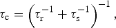 $$\tau _{\rm c} = \left( {\tau _{\rm r}^{ - 1} + \tau _{\rm s}^{ - 1}} \right)^{ - 1}, $$
where τ r is the rotational correlation time of the macromolecule and τ s is the effective electron relaxation time. Values of τ s depend on the nature of the paramagnetic group. Paramagnetic metal ions with anisotropic g-tensors generally exhibit very small values (e.g. τ s ~ 10−13 for anisotropic lanthanides; Otting, Reference Otting2010), thus making τ c ≈ τ s in this case. Nitroxides general exhibit much larger τ s values (~10−6; Bernini et al. Reference Bernini, Venditti, Spiga and Niccolai2009), thus making τ c ≈ τ r in that case. Paramagnetic metal ions with isotropic g-tensors, however, exhibit intermediate values on the same order as τ r (e.g. τ s ~ 10−9 for Mn2+, τ s ~ 10−8 for Gd3+ (Bertini et al. Reference Bertini, Luchinat, Parigi and Pierattelli2005; Iwahara et al. Reference Iwahara, Schwieters and Clore2004b; Pintacuda et al. Reference Pintacuda, Kaikkonen and Otting2004a)), preventing simplification of the expression for τ c.
Under the conditions of biomolecular NMR (where ω s2τ c2 ≫ 1), the high-frequency components of the spectral density function (those dependent on ω S) can be ignored, and the longitudinal and transverse PREs can be expressed by the simplified formulas (Clore & Iwahara, Reference Clore and Iwahara2009):
 $${\rm \Gamma} _1 = \displaystyle{2 \over 5}\left( {\displaystyle{{\mu _0} \over {4\pi}}} \right)^2 \gamma _{\rm I}^2 g^2 \mu _{\rm B}^2 s(s + 1)J_{{\rm SB}} (\omega _{\rm I} ),$$
 $${\rm \Gamma} _2 = \displaystyle{1 \over {15}}\left( {\displaystyle{{\mu _0} \over {4\pi}}} \right)^2 \gamma _{\rm I}^2 g^2 \mu _{\rm B}^2 s(s + 1)\left\{ {4J_{{\rm SB}} (0) + 3J_{{\rm SB}} (\omega _{\rm I} )} \right\}.$$
A paramagnetic group can also cause enhanced relaxation through Curie spin relaxation, which arises from the interaction between the nucleus and the time-averaged magnetization of the electrons (due to the Boltzmann population difference in electron spins states; Bertini et al. Reference Bertini, Luchinat and Parigi2001a). The Γ2 rate due to Curie spin relaxation is given by (Gueron, Reference Gueron1975):
 $${\rm \Gamma} _{2,{\rm Curie}} = \displaystyle{1 \over 5}\left( {\displaystyle{{\mu _0} \over {4\pi}}} \right)^2 \displaystyle{{\left( {\omega _{\rm I}^2 g^4 \mu _{\rm B}^4 s^2 (s + 1)^2} \right)} \over {(3k_{\rm B} T)^2 r^6}} \left\{ {4\tau _{\rm r} + \displaystyle{{3\tau _{\rm r}} \over {1 + (\omega _{\rm I} \tau _{\rm r} )^2}} - 4\tau _{\rm c} - \displaystyle{{3\tau _{\rm c}} \over {1 + (\omega _{\rm I} \tau _{\rm c} )^2}}} \right\}.$$
Note that Curie spin relaxation is independent of the rate of electron relaxation (τ s).
Equations (46)–(48) show that the PRE has an r −6 dependence on the distance between the observed nucleus and the paramagnetic center. The dependence on the magnetic field and on the size of the molecule, however, is slightly more complicated. The dipole–dipole Γ2 rate is approximately independent of field, whereas the Curie Γ2 rate is approximately proportional to the square of the magnetic field. (The dipole–dipole Γ1 rate decreases with increasing field strength.) In cases where τ c ≈ τ r – due to a relatively long τ s (e.g. nitroxide spin radicals) – Curie spin relaxation is negligible, and the Γ2 rate is therefore independent of field. In these cases, the dipole–dipole Γ2 rate is directly proportional to τ r (and to molecular weight). On the other hand, for metal ions with a very short τ s (especially those with an anisotropic g-tensor, e.g. Fe3+, Dy3+), the Γ2 rate in macromolecules is dominated by Curie-spin relaxation. In these cases, the Curie-spin Γ2 rate is also directly proportional to τ r, while the dipole–dipole Γ2 rate is independent of molecular weight because τ c ≈ τ s. For isotropic metal ions, though, such as Mn2+ and Gd3+, the contribution from Curie-spin relaxation is minor, and negligible for medium-sized macromolecules (<40 kDa). For example, in the 20 kDa complex of SRY and DNA–EDTA–Mn2+, Curie-spin relaxation contributed 2% of the Γ2 rates at a 1H-frequency of 800 MHz and a temperature of 308 K (Iwahara et al. Reference Iwahara, Tang and Clore2007). However, for a larger molecule (>100 kDa), Curie-spin relaxation can contribute more than 20% of the total value of Γ2 under these conditions (Clore & Iwahara, Reference Clore and Iwahara2009).
Thus, for measuring PREs, it is advantageous to use a paramagnetic group with an isotropic g-tensor because the Curie spin contribution to the Γ2 rate will be much less (often negligible) compared with one with an anisotropic g-tensor. In addition, for an anisotropic paramagnetic group, the generation of PCSs means that the chemical shifts (and therefore resonance assignments) are altered and that exchange contributions are different between the diamagnetic and paramagnetic samples, which complicates analysis, as described below (Clore & Iwahara, Reference Clore and Iwahara2009).
Artificially introduced paramagnetic groups are generally attached to the macromolecule of interest through linkers that have several rotatable bonds. Hence, these paramagnetic centers are intrinsically flexible. In addition, the observed nuclei may be located in mobile regions of the macromolecule. The effect of fast dynamics in the picosecond to nanosecond timescale on the PRE for paramagnetic systems with an isotropic g-tensor can be readily taken into account by modifying the SB equations described above by incorporating a ‘model-free’ formalism (SBMF) (Lipari & Szabo, Reference Lipari and Szabo1982a). This transforms the spectral density function in Eq. (44) into (Iwahara et al. Reference Iwahara, Schwieters and Clore2004b):
 $$J_{{\rm SBMF}} (\omega ) = \left\langle {r^{ - 6}} \right\rangle \left\{ {\displaystyle{{{\bi S}^2 \tau _{\rm c}} \over {1 + (\omega \tau _{\rm c} )^2}} + \displaystyle{{(1 - {\bi S}^2 )\tau _{\rm t}} \over {1 + (\omega \tau _{\rm t} )^2}}} \right\},$$
where S2 is the square of the generalized order parameter, 〈r −6〉 is the population-averaged distance inverse sixth power of the distance between the paramagnetic center and the observed nucleus, and τ t is the total correlation time, defined as:
 $$\tau _{\rm t} = \left( {\tau _{\rm r}^{ - 1} + \tau _{\rm s}^{ - 1} + \tau _{\rm i}^{ - 1}} \right)^{ - 1}, $$
where τ i is the correlation time for internal motion. These equations are valid for isotropically tumbling systems; otherwise, the angles between the principal axes of the diffusion tensor and PRE vector must be taken into account (Benetis & Kowalewski, Reference Benetis and Kowalewski1985; Woessner, Reference Woessner1962).
The model-free formalism is most commonly employed for analyzing relaxation due to fixed-length dipole–dipole interactions, such as those in 1H–15N or 1H–13C bond vectors. However, it can also be applied to variable-length vectors (e.g. PRE; Iwahara et al. Reference Iwahara, Schwieters and Clore2004b), where it takes the form (Olejniczak et al. Reference Olejniczak, Dobson, Karplus and Levy1984):
 $${\bi S}^2 = \displaystyle{{4\pi} \over 5}\left\langle {r^{ - 6}} \right\rangle ^{ - 1} \sum\limits_{m = - 2}^2 {\left\vert {\left\langle {\displaystyle{{Y_2^m {\rm \Omega} ^{{\rm mol}}} \over {r^3}}} \right\rangle} \right\vert^2}, $$
where Y 2m(Ω) are second-order spherical harmonics and Ωmol are Euler angles in the molecular frame. The order parameter can be approximated by decomposing it into its radial and angular components, as has been demonstrated for 1H–1H dipolar interactions (Bruschweiler et al. Reference Bruschweiler, Roux, Blackledge, Griesinger, Karplus and Ernst1992):
 $${\bi S}^2 \approx {\bi S}_{{\rm angular}}^2 {\bi S}_{{\rm radial}}^2, $$
where the angular (S angular2) and radial (S radial2) order parameters are defined as:
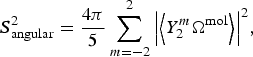 $${\bi S}_{{\rm angular}}^2 = \displaystyle{{4\pi} \over 5}\sum\limits_{m = - 2}^2 {\left\vert {\left\langle {Y_2^m {\rm \Omega} ^{{\rm mol}}} \right\rangle} \right\vert^2}, $$
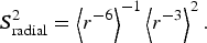 $${\bi S}_{{\rm radial}}^2 = \left\langle {r^{ - 6}} \right\rangle ^{ - 1} \left\langle {r^{ - 3}} \right\rangle ^2. $$
These relationships are used directly for back-calculating PRE values from known structures (and for refining against PRE data) as described below. The PRE measured for a given nucleus has a population-weighted 〈r −6〉 dependence on the distance between the nucleus and the paramagnetic center, hence its utility as a structural restraint (and as a probe of minor states) emerges. However, because most paramagnetic tags used for measuring PRE are highly flexible (and the molecules of interest are also often quite flexible), it is important in structure calculations to refine directly against the PRE data (e.g. using prePot in Xplor-NIH (Iwahara et al. Reference Iwahara, Schwieters and Clore2004b) as discussed below) rather than converting PRE data into a single distance, which is generally incorrect (although PRE calculators have been made available online at spin.niddk.nih.gov/clore for qualitative purposes).
Both the transverse and longitudinal PREs are influenced by internal motion (Iwahara et al. Reference Iwahara, Schwieters and Clore2004b). However, while Γ1 has a complicated dependence on the internal correlation time, the Γ2 shows a simpler dependence. As the internal correlation time is increased from 0 (infinitely fast internal motion) to a value greater than the overall rotational correlation time, the ratio Γ2,SBMF/Γ2,SB (where Γ2,SBMF is Γ2 calculated from the SBMF equation, and Γ2,SB is Γ2 calculated from the SB equation) increases from the value of the order parameter (0 ≤ S2 ≤ 1) to 1. For the longitudinal PRE, however, Γ1,SBMF/Γ1,SB first increases from the value of S2 when τ i = 0, up to a maximum value ≫ 1 when τ i ≈ 1/ω (where ω is the resonance frequency of the observed nucleus in rad s−1), before eventually approaching 1 (Iwahara et al. Reference Iwahara, Schwieters and Clore2004b). Thus, whereas a simple estimation of τ i is sufficient for structural analysis of 1H–Γ2 data, such treatment of 1H–Γ1 data requires accurate information on τ i for individual PRE vectors (Iwahara & Clore, Reference Iwahara and Clore2010). Another complication is that, due to cross-relaxation and water exchange, 1H R 1 relaxation does not follow a single-exponential curve. Thus, it is advantageous to measure the transverse PRE instead of the longitudinal PRE. For very fast motion (τ i ≪ τ r; i.e. picosecond timescale motion), the transverse PRE is virtually independent of the internal correlation time, and the order parameter acts as a scaling factor. In either case, though, the SBMF equations reduce to the SB equations under conditions where the internal motion is either very slow (τ t ≈ τ c) or highly restricted in space (S2 ≈ 1).
3.1.2 PRE from minor states
In a system undergoing exchange between states on a fast timescale, the overall PRE profile observed for the ensemble of states is the population-weighted average of all the members of the ensemble. Owing to the 〈r −6〉 distance dependence of the PRE, such a profile will be dominated by the states in which the paramagnetic center more closely approaches the observed nuclei. Thus, even if a state occupies a small (<10%) portion of the total population, it can be readily detected if it involves a shorter distance between a paramagnetic probe and reporter than the other state(s) (Fig. 2). Thus, an otherwise invisible minor state can be detected and structurally characterized using PRE (Clore & Iwahara, Reference Clore and Iwahara2009).
Under fast exchange conditions on the PRE timescale (i.e. the rate of exchange between the species is much greater than the difference in PRE rates between states) the overall PRE observed for a nucleus is given by:
 $${\rm \Gamma} _2^{{\rm app}} = \sum {\,p_i {\rm \Gamma} _{2,i}}, $$
where Γ2app is the apparent transverse PRE measured for the entire ensemble, Γ2,i is the transverse PRE for state i, and p i is the population of state i. Eq. (55) holds when the rate of exchange is slower than the overall correlation time (k ex ≪ 1/τ c); in the limit of ultrafast exchange, however, where k ex ≫ 1/τ c, in Eq. (55) would be replaced by 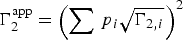 ${\rm \Gamma} _2^{{\rm app}} = \left(\sum {\,p_i \sqrt{{\rm \Gamma} _{2,i}}\hskip 1pt}\right) ^2$ (i.e. under ultrafast exchange conditions the contribution of each state to
 ${\rm \Gamma} _2^{{\rm app}}$ is roughly proportional to the square of its population due to the fact that individual components of
 ${\rm \Gamma} _2^{{\rm app}}$ are averaged as <r −3> as opposed to <r −6> under the more usual conditions of Eq. (55)).
In the case of two-state exchange between a major state (A) and a minor state (B), the apparent observed PRE is given by:
 $${\rm \Gamma} _2^{{\rm app}} = p_{\rm A} {\rm \Gamma} _{2,{\rm A}} + p_{\rm B} {\rm \Gamma} _{2,{\rm B}}. $$
If the exchange between states A and B is not fast on the PRE timescale (i.e. if k ex ≫ Γ2,B − Γ2,A is not true), the apparent PRE is not simply a population-averaged value, but is instead intermediate between Γ2,A and the population-averaged value (Fig. 2c). Under these conditions of slower exchange, the apparent PRE can be calculated using the McConnell equations (McConnell, Reference Mcconnell1958). These necessary equations are identical to the general equations for chemical exchange (Eqs. (16)–(20)), except the relaxation matrix R (Eq. (18)) includes the PRE from each state, taking the form (for two-site exchange):
 $${\bf R =} \left[ {\matrix{ {R_{2,{\rm A}} + {\rm \Gamma} _{2,{\rm A}}} & 0 \cr 0 & {R_{2,{\rm B}} + {\rm \Gamma} _{2,{\rm B}}} \cr}} \right].$$
Apparent relaxation rates can be extracted by fitting the line shape of the Fourier-transformed solution of the McConnell equations. Under such cases, where exchange takes place on the intermediate PRE timescale (k ex ≈ Γ2,B − Γ2,A), the apparent PRE measured for a system in exchange between two states, in addition to encoding distance and population information, also encodes kinetic information, although in practice it is difficult to extract this information from PRE data alone.
To visualize how PRE can be used to detect and characterize a minor state, consider a protein in exchange between two states (Fig. 2). In state A, the protein is in a more extended conformation, and the distance between the two selected points is 40 Å. In state B, however, the protein is in a more compact conformation, and the distance between these same two points is 8 Å. If one of the points is a paramagnetic center, and the other is a 1H nucleus, we can calculate the PRE (after specifying the correlation times and the order parameter of the vector between the paramagnetic center and the observed nucleus). In this example, we will consider a single unpaired electron (e.g. a nitroxide spin label), and we will set τ c = 10 ns (corresponding to a protein at room temperature with a molecular weight of ~20 kDa). Also, we will assume that the paramagnetic center/observed nucleus vector is rigid, although this is not the case for most conventional spin labels (e.g. MTSL). For state A, with the nucleus far from the unpaired electron, Γ2,A = 0·12 s−1 (effectively zero). However, in state B, where they are in much closer proximity, Γ2,B = 1900 s−1.
If the protein in this example is in fast exchange between states A and B (k ex ≫ Γ2,A − Γ2,B = 1900 s−1; τ ex ≪ 500 μs), the apparent PRE would be the population-weighted average of Γ2,A and Γ2,B (Eq. (56)). Thus, even if state A comprises 99% of the total population, and state B only comprises 1% of the total population, Γ2app = 0·99 × 0·12 s−1 + 0·01 × 1900 s−1 ≈ 19 s−1. Thus, even though state B comprises only 1% of the total population, Γ2app arises almost exclusively from the minor state.
Two conditions are necessary for detection of a minor state by PRE: (1) a shorter distance between probe and reporter in the minor state, and (2) fast exchange between the states. Having a shorter distance to measure in the minor state is a necessary requirement for PRE measurements on minor states, and detecting such a state is most straightforward for the transient association between two molecules or for a minor state that involves forming a more compact structure than in the major state (e.g. CaM; Anthis et al. Reference Anthis, Doucleff and Clore2011). However, other states can also be measured, as long as a paramagnetic probe position can be found where at least some measurable nuclei are in closer proximity to the probe in the minor state than in the major state.
For quantitative PRE measurements (i.e. for the overall measured PRE profile to be exactly the population-weighted average of the PRE profiles from the individual states), the rate of exchange (k ex = k AB + k BA) must be fast on the PRE timescale, meaning that k ex ≫ Γ2,B − Γ2,A. Otherwise, the apparent PRE becomes highly dependent on k ex, as seen in Fig. 2. That being said, under conditions where k ex ~ Γ2,B − Γ2,A, the Γ2obsrate is only decreased by a factor of about 2 relative to the limiting value in the fast exchange limit (Fig. 2c); given the 〈r −6〉 dependence of the PRE, the assumption of fast exchange in the intermediate PRE regime would only result in a ~10% overestimation in the corresponding distance. As the exchange rate decreases, the apparent PRE decreases, eventually becoming equal to that of state A, providing no information on the minor state. If exchange is not fast on the PRE timescale, the apparent PRE also becomes dependent on the chemical shift difference between states A and B (ΩA − ΩB), decreasing with decreasing k ex or increasing ΩA − ΩB (unless k ex ≫ |ΩA − ΩB|) (Clore & Iwahara, Reference Clore and Iwahara2009). However, under these conditions, the peak will also be subject to additional line broadening, making measurements difficult or impossible as |ΩA − ΩB| approaches k ex. If k ex ≪ |ΩA − ΩB|, then the two states will display two separate peaks; the minor state peak will likely be invisible, and the major state peak will not contain PRE information on the minor state (Clore & Iwahara, Reference Clore and Iwahara2009).
3.2 Data acquisition
PRE data are acquired by measuring transverse relaxation rates for a paramagnetic sample and a diamagnetic sample. Subtraction of the diamagnetic R 2 from the paramagnetic R 2 for each nucleus yields its PRE rate Γ2. The molecule of interest must be either recombinantly expressed (often in E. coli) or chemically synthesized and then tagged with a paramagnetic label (or, if a natural paramagnetic ion ligand will be used, it must be added to the protein via a chelating group or an intrinsic metal-binding site). The protein will usually be universally or selectively 15N- and/or 13C-labeled to perform measurements using modern multidimensional heteronuclear NMR spectroscopy. For intermolecular PRE measurements, one can use a 15N/13C-labeled protein without a paramagnetic tag in the presence and absence of a non-isotopically labeled (natural abundance) protein with a paramagnetic tag. It is advisable to perform experiments on perdeuterated proteins because the 1Hα–1HN coupling can influence the PRE measurements, but if using perdeuterated proteins is not feasible, this coupling can largely be cancelled by appropriate design of the pulse sequence (Iwahara et al. Reference Iwahara, Anderson, Murphy and Clore2003, Reference Iwahara, Tang and Clore2007).
3.2.1 Producing paramagnetic samples
Broadly speaking, two types of paramagnetic labels are available for measuring PREs: those containing a nitroxide group and those that act as a ligand for a paramagnetic cation (e.g. Mn2+, Cu2+, and Gd3+). If a protein has an intrinsic cation-binding site, a paramagnetic cation can often be introduced in place of the natural metal ligand. For proteins that are not native metalloproteins, short metal-binding sequences can be genetically encoded. Examples of such sequences include the N-terminal ATCUN motif (XXH), which binds paramagnetic Cu2+ (Donaldson et al. Reference Donaldson, Skrynnikov, Choy, Muhandiram, Sarkar, Forman-Kay and Kay2001), the sequence YVDTNNDGAYEGDEL, which specifically binds lanthanides (Wohnert et al. Reference Wohnert, Franz, Nitz, Imperiali and Schwalbe2003), and the N-terminal sequence HHP, which forms a dimer with two peptides bound to paramagnetic Ni2+ (Jensen et al. Reference Jensen, Lauritzen, Dahl, Pedersen and Led2004). A paramagnetic Cu2+ ion can also be introduced into a protein by making a double histidine mutation at i and i + 4 positions in an α-helix and then adding the chelating agent nitrilotriacetic acid in a 1:1 ratio with Cu2+ (which prevents Cu2+-mediated dimerization) (Liu et al. Reference Liu, Gong, Guo, Zhang and Tang2014).
The most common method for attaching a paramagnetic probe to a protein of interest is site-directed spin labeling (Hubbell et al. Reference Hubbell, Cafiso and Altenbach2000; Todd et al. Reference Todd, Cong, Levinthal, Levinthal and Hubbell1989), where a paramagnetic tag is conjugated to an exposed cysteine residue introduced by site-directed mutagenesis (Fig. 6). Conjugation by disulfide chemistry (Battiste & Wagner, Reference Battiste and Wagner2000; Dvoretsky et al. Reference Dvoretsky, Gaponenko and Rosevear2002; Gaponenko et al. Reference Gaponenko, Howarth, Columbus, Gasmi-Seabrook, Yuan, Hubbell and Rosevear2000) offers high specificity for cysteine and is straightforward to perform using a spin label molecule with a methanethiosulfonate or pyridylthiol functional group (Fig. 6a). Disulfide linkages are somewhat unstable, and over time some of the paramagnetically tagged protein is replaced by disulfide cross-linked protein dimers, although over a short time period (up to ~1 month, often longer), the disulfide-conjugated paramagnetic protein sample is pure and stable enough to perform PRE measurements. Paramagnetic probes can also be conjugated using iodo- or bromoacetamide derivatives, which irreversibly form a C–S bond with cysteine (Gillespie & Shortle, Reference Gillespie and Shortle1997b; Ogawa & McConnel, Reference Ogawa and Mcconnel1967) (Fig. 6b); however, although they are advantageous for their exceptional stability, they exhibit lower specificity (also reacting at a slower rate with histidine, methionine, and lysine). Maleimide derivatives, however, are not recommended due to their instability (Kosen, Reference Kosen1989) (Fig. 6c). As these tags conjugate to exposed cysteine residues, any natural exposed cysteine residues will need to be mutated to serine or alanine. Even buried cysteines can become transiently exposed by the protein's intrinsic motions, so one will need to ensure that they do not react with the tag if they are to remain unmutated.
Site-directed spin labeling. Shown are four different chemistries for conjugating a spin label to a cysteine residue (a–c) or to an unnatural amino acid (d). All four examples are nitroxide spin labels (with the unpaired electron denoted with a dot), but the same chemistry can be used for spin labels that chelate a paramagnetic metal ion. The Cα of the peptide backbone is labeled. (a) Reaction of a methanethiosulfonate with cysteine to form a disulfide bond. The compound (1-oxyl-2,2,5,5-tetramethyl-∆3-pyrroline-3-methyl) methanethiosulfonate (MTSL; left) reacts with cysteine to form the R1 side chain (right) (Battiste & Wagner, Reference Battiste and Wagner2000; Gaponenko et al. Reference Gaponenko, Howarth, Columbus, Gasmi-Seabrook, Yuan, Hubbell and Rosevear2000). (b) Reaction of an iodoacetamide with cysteine to form an S–C bond. Shown on the left is 3-(2-iodoacetamido)-2,2,5,5-tetramethyl-1-pyrolidinyloxy (iodoacetamido-PROXYL) (Gillespie & Shortle, Reference Gillespie and Shortle1997a). (c) Reaction of a maleimide with cysteine to form an S–C bond. Shown on the left is N-(1-oxyl-2,2,6,6-tetramethyl-4-piperidinyl) maleimide (maleimide-TEMPO) (Griffith & McConnell, Reference Griffith and Mcconnell1966; Tang et al. Reference Tang, Ghirlando and Clore2008a). (d) Reaction of 3-aminooxymethyl-2,2,5,5-tetramethyl-2,5-dihydro-1H-pyrrol-1-yloxyl radical (HO-4120) with the unnatural amino acid p-acetyl-l-phenylalanine to form the side chain K1 (Fleissner et al. Reference Fleissner, Brustad, Kalai, Altenbach, Cascio, Peters, Hideg, Peuker, Schultz and Hubbell2009).
An alternative method, which is especially useful when the removal of natural cysteines is difficult or impossible, involves the incorporation of an unnatural amino acid using an orthogonal-tRNA/aminoacyl-tRNA synthetase pair (Wang et al. Reference Wang, Brock, Herberich and Schultz2001). The spin label site is generated by introducing an amber (TAG) codon into the DNA sequence of the protein of interest by site-directed mutagenesis. The protein is then coexpressed with the unnatural tRNA/aminoacyl-tRNA synthetase pair. This method can be used to produce a protein containing the unnatural amino acid p-acetyl-l-phenylalanine, which can be conjugated to HO-4120, a hydroxylamine-functionalized nitroxide spin-label (Fleissner et al. Reference Fleissner, Brustad, Kalai, Altenbach, Cascio, Peters, Hideg, Peuker, Schultz and Hubbell2009) (Fig. 6d). This method has been used to produce spin-labeled proteins at high yields, even in perdeuterated media, where it has been demonstrated that the key for sufficient yields is to induce expression of the tRNA/aminoacyl-tRNA synthetase pair while still in rich, protonated media before changing to deuterated media for expression of the target protein (Venditti et al. Reference Venditti, Fawzi and Clore2012). For shorter sequences (up to ~50 residues), a spin-labeled amino acid can be directly incorporated through solid-phase peptide synthesis (Hanson et al. Reference Hanson, Millhauser, Formaggio, Crisma and Toniolo1996; Lindfors et al. Reference Lindfors, De Koning, Drijfhout, Venezia and Ubbink2008; Milov et al. Reference Milov, Tsvetkov, Gorbunova, Mustaeva, Ovchinnikova and Raap2002; Monaco et al. Reference Monaco, Formaggio, Crisma, Toniolo, Hanson, Millhauser, George, Deschamps and Flippen-Anderson1999a, Reference Monaco, Formaggio, Crisma, Toniolo, Hanson and Millhauserb; Shenkarev et al. Reference Shenkarev, Paramonov, Balashova, Yakimenko, Baru, Mustaeva, Raap, Ovchinnikova and Arseniev2004).
Some spin label advances have been summarized in recent reviews (Hubbell et al. Reference Hubbell, Lopez, Altenbach and Yang2013; Jeschke, Reference Jeschke2013; Keizers & Ubbink, Reference Keizers and Ubbink2011), and Fig. 7 shows some nitroxide and metal-chelating paramagnetic tags. The paramagnetic nitroxide side chain R1, which is formed by disulfide conjugation of the spin label MTSL to cysteine (Fig. 7a; Battiste & Wagner, Reference Battiste and Wagner2000; Gaponenko et al. Reference Gaponenko, Howarth, Columbus, Gasmi-Seabrook, Yuan, Hubbell and Rosevear2000), is commonly used in EPR studies and has been used to measure PREs in several studies (Anthis & Clore, Reference Anthis and Clore2013; Anthis et al. Reference Anthis, Doucleff and Clore2011; Bermejo et al. Reference Bermejo, Strub, Ho and Tjandra2009; Fawzi et al. Reference Fawzi, Fleissner, Anthis, Kalai, Hideg, Hubbell and Clore2011a; Volkov et al. Reference Volkov, Worrall, Holtzmann and Ubbink2006). For studies involving R1, an acylated diamagnetic control is available (Fig. 7b). Alternatively, for PRE measurements, an EDTA-based tag (Fig. 7e), which can chelate a paramagnetic ion (e.g. Mn2+) or a diamagnetic control (e.g. Ca2+), can be used (Dvoretsky et al. Reference Dvoretsky, Gaponenko and Rosevear2002; Ebright et al. Reference Ebright, Chen, Pendergrast and Ebright1992; Ermacora et al. Reference Ermacora, Delfino, Cuenoud, Schepartz and Fox1992). Such tags have the advantage of giving larger PRE values due to larger electron spin number. However, these metal-bound tags are problematic for PCS studies because their flexibility greatly complicates analysis of PCSs, which are orientation dependent. Additionally, metal-bound EDTA forms two stereoisomers, each with a slightly different χ-tensor, causing the appearance of multiple peaks due to slow metal/tag exchange (Ikegami et al. Reference Ikegami, Verdier, Sakhaii, Grimme, Pescatore, Saxena, Fiebig and Griesinger2004; Pintacuda et al. Reference Pintacuda, Moshref, Leonchiks, Sharipo and Otting2004b; Vlasie et al. Reference Vlasie, Comuzzi, Van Den Nieuwendijk, Prudencio, Overhand and Ubbink2007). Metal-binding tags have also been developed with multiple functionalities, for example 4′-mercapto-2,2′:6′,2″-terpyridine-6,6″-dicarboxylic acid (4MTDA), which binds to lanthanides and can be used for the measurement of PRE and PCSs, but also fluoresces in the UV–vis range (Huang et al. Reference Huang, Pei, Zuo, Chen, Yang and Su2013).
Spin label side chains for measuring PRE. Shown are three nitroxide spin label side chains (a, c, d), a diamagnetic control (b), and two side chains for chelating paramagnetic metal ions (e, f). The unpaired electron in each nitroxide side is denoted with a dot, and metal chelating sites are denoted with stars. The Cα of the peptide backbone is labeled. (a) The side chain R1, introduced by the reaction of (1-oxyl-2,2,5,5-tetramethyl-∆3-pyrroline-3-methyl) methanethiosulfonate (MTSL) with a cysteine side chain (Battiste & Wagner, Reference Battiste and Wagner2000; Gaponenko et al. Reference Gaponenko, Howarth, Columbus, Gasmi-Seabrook, Yuan, Hubbell and Rosevear2000). (b) An acylated derivative of R1, which can be used as a diamagnetic control for R1/MTSL PRE studies, introduced by the reaction of (1-acetoxy-2,2,5,5-tetramethyl-δ-3-pyrroline-3-methyl) methanethiosulfonate with a cysteine side chain (Altenbach et al. Reference Altenbach, Oh, Trabanino, Hideg and Hubbell2001). (c) The side- chain R1p, a derivative of R1 that adopts a narrower range of conformations and simplifies analysis, introduced by the reaction of 3-methanesulfonilthiomethyl-4-(pyridin-3-yl)-2,2,5,5-tetramethyl-2,5-dihydro-1H-pyrrol-1-yloxyl radical (HO-3606) with a cysteine side chain (Fawzi et al. Reference Fawzi, Fleissner, Anthis, Kalai, Hideg, Hubbell and Clore2011a). (d) The side chain RX, which also is more rigid than R1, introduced by the reaction of 3,4-bis-(methanethiosulfonylmethyl)-2,2,5,5-tetramethyl-2,5-dihydro-1H-pyrrol-1-yloxy radical (HO-1944) with two cysteine side chains located within close proximity (specifically at i and i + 3 or i + 4 in a helix or at i and i + 2 in a β-strand) (Fleissner et al. Reference Fleissner, Bridges, Brooks, Cascio, Kalai, Hideg and Hubbell2011). (e) A side chain for chelating paramagnetic metal ions (e.g. Mn2+) or diamagnetic controls (e.g. Ca2+), introduced by the reaction of S-(2-pyridylthio)cysteaminyl-EDTA with a cysteine side chain (Dvoretsky et al. Reference Dvoretsky, Gaponenko and Rosevear2002; Ebright et al. Reference Ebright, Chen, Pendergrast and Ebright1992; Ermacora et al. Reference Ermacora, Delfino, Cuenoud, Schepartz and Fox1992). (f) The CLaNP (caged lanthanide NMR probe) tags chelate lanthanide ions and offer a more rigid paramagnetic center, suitable for both PRE and PCS measurements. Shown here is the side chain introduced by conjugating 1,4,7,10-tetraazacyclododecane-1,7-[di-(N-oxido-pyridine-2-yl)methyl]-4,10-bis(2-(acetylamino)ethylmethanesulfonothioate) (CLaNP-5) to two cysteine side chains located in close proximity to one another (Keizers et al. Reference Keizers, Desreux, Overhand and Ubbink2007, Reference Keizers, Saragliadis, Hiruma, Overhand and Ubbink2008).
A cysteine-conjugated MTSL tag (i.e. residue R1; Fig. 7a), has five torsional angles about which rotation is possible. This allows the tag to sample a large range of conformational space and makes it highly dynamic (Bridges et al. Reference Bridges, Hideg and Hubbell2010; Chou et al. Reference Chou, Case and Bax2003) (overall correlation time of the order of ~0·7 ns (Oganesyan, Reference Oganesyan2011)). However, the use of a shorter spin label increases the likelihood of undesired perturbations to the structure or dynamics of the molecule under study (Jeschke, Reference Jeschke2013). Thus, whereas the dynamics of the spin label have complicated analysis and impeded progress in the past, newer computational methods described below have made it possible to take these dynamics into account, making it preferable to use the more flexible tag that is less likely to disrupt the protein under study. NMR studies attempting to quantitatively interpret the PREs arising from R1 (Bermejo et al. Reference Bermejo, Strub, Ho and Tjandra2009), like any other label with internal motions, must take into account the ensemble of nitroxide positions, their interconversion dynamics, and the order parameters for the interspin (nitroxide–nucleus) vectors (Clore & Iwahara, Reference Clore and Iwahara2009; Iwahara et al. Reference Iwahara, Schwieters and Clore2004b).
Various analogs of R1 (Columbus et al. Reference Columbus, Kalai, Jeko, Hideg and Hubbell2001) have shown reduced flexibility, thus potentially simplifying analysis. A series of R1 analogs aromatically substituted at position 4 of the paramagnetic pyrroline ring exhibit restricted motion, and the 4-pyridyl analog of R1 (R1p; Fig. 7c) shows particular promise. In one study, multiple tag conformations were required to fit PRE data from R1, but a single conformation could be used for the R1p tag (Fawzi et al. Reference Fawzi, Fleissner, Anthis, Kalai, Hideg, Hubbell and Clore2011a). A different nitroxide side chain (V1), formed by the reaction between a free cysteine and bis(2,2,5,5-tetramethyl-3-imidazoline-1-oxyl-4-il)-disulfide (IDSL), also displays more constrained geometry than R1 (Toledo Warshaviak et al. Reference Toledo Warshaviak, Khramtsov, Cascio, Altenbach and Hubbell2013). If two cysteines are available in close proximity (at i and i + 3 or i + 4 in a helix or at i and i + 2 in a β-strand), the side chain RX (Fig. 7d) can be introduced, forming two disulfide linkages and maintaining a more rigid conformation than R1 (Fleissner et al. Reference Fleissner, Bridges, Brooks, Cascio, Kalai, Hideg and Hubbell2011). An alternative strategy for a more rigid tag is the incorporation of the unnatural amino acid TOAC into the peptide of interest for PRE studies (Lindfors et al. Reference Lindfors, Venkata, Drijfhout and Ubbink2011). TOAC contains a nitroxide radical that is contained within a single piperidine ring that includes the backbone Cα. Its downsides are that it can only be incorporated into synthetic peptides (not recombinant proteins), and it can still adopt multiple conformations (Crisma et al. Reference Crisma, Deschamps, George, Flippen-Anderson, Kaptein, Broxterman, Moretto, Oancea, Jost, Formaggio and Toniolo2005; Flippen-Anderson et al. Reference Flippen-Anderson, George, Valle, Valente, Bianco, Formaggio, Crisma and Toniolo1996).
More rigid tags have also been designed to introduce paramagnetic lanthanides into proteins via chelating groups. These are particularly valuable for PCS studies, where rigid electron–nucleus vectors are needed due to the orientational dependence of the PCS. A series of CLaNP (caged lanthanide NMR probe) tags have been developed, which form a much more rigid structure. After chelating a lanthanide ion, the CLaNP tag can then be conjugated to a protein via two cysteine residues in close proximity on the surface of the protein. One of these, CLaNP-5 (Keizers et al. Reference Keizers, Desreux, Overhand and Ubbink2007, Reference Keizers, Saragliadis, Hiruma, Overhand and Ubbink2008) is shown in Fig. 7f. CLaNP-7, has a pH-dependent χ-tensor and has a lower charge (+1 versus +3 for CLaNP-5), lessening the potential for electrostatic interactions with negatively charged molecules (Liu et al. Reference Liu, Keizers, Hass, Blok, Timmer, Sarris, Overhand and Ubbink2012). Another tag, 4-mercaptomethyl-dipicolinic acid, adopts a rigid conformation after conjugation to a surface cysteine located near a carboxyl-bearing side chain, followed by addition of a lanthanide ion (Shen et al. Reference Shen, Vernon, Baker and Bax2009). Another strategy for introducing a paramagnetic lanthanide uses stereospecifically methylated DOTA (DOTA-M8), which is conjugated to the protein via a single surface cysteine, and adopts a more rigid conformation due to hydrophobic interactions on the protein surface (Haussinger et al. Reference Haussinger, Huang and Grzesiek2009).
It is essential to ensure that the introduction of the mutation and the introduction of the tag do not affect the structure or function of the protein. This can preferably be done through a functional assay if one is available. Biophysical measures (e.g. CD, melting temperature) can be used to ensure that there are no changes to protein structure or stability. If the protein is not expressed or becomes insoluble, this likely indicates that the mutation has disrupted the structure of the protein and made it unstable. If it is possible to acquire an NMR spectrum (e.g. 1H–15N HSQC) of the mutant protein and compare it to the spectrum of the wild-type protein, there should not be any broadened or disappearing peaks, and only peaks near the site of the mutation should exhibit changes in chemical shift. One can then check a spectrum of the protein conjugated to a diamagnetic tag. These results should also be the same. Some very localized disruption of the protein structure may be inevitable and they can be considered acceptable if they are restricted to adjacent residues. When PRE data are acquired, the R 2 rate of the diamagnetic control should not vary from that of the wild type. Enhancements to the diamagnetic R 2 can indicate some disruption of local structure. Any significant disruption needs to be taken into account and may indicate that a particular tag position is not appropriate. Finding the best sites for a paramagnetic tag often involves trial and error, as tags at various different positions may cause disruptions to protein structure.
3.2.2 Measuring PRE data
The transverse PRE rate (Γ2) of a nucleus is given by the difference in its transverse relaxation rate between the paramagnetic (R 2,para) and diamagnetic (R 2,dia) states of the molecule:
 $${\rm \Gamma} _2 = R_{2,{\rm para}} - R_{2,{\rm dia}} $$
The PRE is determined by measuring R 2 values for a paramagnetic sample and for a diamagnetic sample and then subtracting the diamagnetic R 2 values from the paramagnetic R 2 values. The most appropriate diamagnetic sample will depend on the nature of the paramagnetic sample. If the PREs arise from a paramagnetic ion, an appropriate diamagnetic control would be a similar sample with the paramagnetic ion replaced with a diamagnetic ion of similar properties. For a metalloprotein, this might be the natural metal ligand. Or, for a chelating extrinsic tag for example, one could use Mn2+ for the paramagnetic sample and Ca2+ for the diamagnetic sample. For a protein tagged with a nitroxide label, a good diamagnetic sample is a protein tagged with a similar diamagnetic label. For MTSL, one could use an acylated analogous tag ((1-acetoxy-2,2,5,5-tetramethyl-δ-3-pyrroline-3-methyl) methanethiosulfonate) for the diamagnetic control. An alternative is to add ascorbic acid directly to the paramagnetic sample, which reversibly reduces nitroxides, forming a diamagnetic product. This method has the advantage of only requiring one sample, but has the downside of requiring a large excess of ascorbic acid, which must remain present during acquisition (Venditti et al. Reference Venditti, Fawzi and Clore2011). These methods are generally preferable, however, to using a wild-type or untagged protein as the diamagnetic control, as the tag can have subtle local effects that will not be taken into account in the wild-type protein.
Commonly, one measures the PRE of the backbone amide protons (1HN) using a 2D 1H–15N HSQC-based pulse sequence (Iwahara et al. Reference Iwahara, Tang and Clore2007). Two examples are shown in Fig. 8. In the first example (Fig. 8a), the period for the 1H transverse relaxation measurement (T) is incorporated in the first INEPT scheme. Identical experiments are performed for the paramagnetic and diamagnetic samples to obtain Γ2. This pulse sequence can readily be modified to a transverse relaxation optimized (TROSY) version, although Boltzmann 15N-magnetization should be destroyed at the beginning the pulse sequence so that all observables are modulated solely by 1H transverse relaxation during the time interval T (Clore & Iwahara, Reference Clore and Iwahara2009). If a TROSY pulse sequence is being used, it is advantageous to measure the slower TROSY R 2 rate for each sample by placing the delay T at the end of the sequence (Fig. 8b). Additionally, 3D experiments can also be employed to overcome peak overlap. HNCO-based experiments measuring 1HN–Γ2 have been developed for this purpose (Anthis et al. Reference Anthis, Doucleff and Clore2011; Hu et al. Reference Hu, Vogeli and Clore2007).
Pulse sequences for 2D 1HN–Γ2 PRE experiments. (a) HSQC-based pulse sequence for measuring 1HN–Γ2. Full details are given in Iwahara et al. (Iwahara et al. Reference Iwahara, Tang and Clore2007). The delay T is incremented to measure 1HN transverse relaxation. Two 180° 15N pulses are applied to eliminate longitudinal cross-correlated relaxation interference between the 15N–1H dipolar interaction and 15N chemical shift anisotropy. Although 3J HN−Hα is active for non-deuterated proteins during the period T, the resulting modulation is cancelled out when Γ2 is measured by the two-time-point method, using an equal delay T in both the paramagnetic experiment and the diamagnetic control. Alternatively, 3J HN−Hα can be directly cancelled by replacing the 180° 1H pulse separating the two halves of delay T (arrow) with an IBURP2 pulse that selectively excites only the amide region of the 1H spectrum. (b) TROSY pulse sequence for measuring 1HN–Γ2. Note that in this pulse sequence the delay T (located at the end of the pulse sequence) is incremented to measure the slower-relaxing TROSY component of the 1HN transverse relaxation rate (although 1HN–Γ2 is the same as for R 2 measurements). For proteins that are not deuterated, 3J HN−Hα can be cancelled out either by employing the two-time-point method or by replacing the final 180° 1H pulse and adjacent soft water flip-back pulses separating the two halves of delay T (arrow) with an IBURP2 pulse that selectively excites only the amide region of the 1H spectrum. Unless otherwise indicated, all pulses have phase x; φ 1 = y, −y, −x, x; φ rec = y, −y, x, −x. Quadrature detection in the indirect 15N dimension is achieved using the Rance-Kay echo/anti-echo scheme (Kay et al. Reference Kay, Keifer and Saarinen1992) by inverting gradients G3 and −G3 and using phase φ 1 = y, −y, x, −x for the second free induction decay (FID) of each quadrature pair.
The 1H–Γ2 PRE can also be measured for protons directly bonded to 13C (Iwahara et al. Reference Iwahara, Schwieters and Clore2004b), and the measurement of methyl 1H–Γ2 can be particularly useful for larger proteins (Fig. 8). (Note that although R 2 for methyl CH3 protons is biexponential due to cross-correlation (Ollerenshaw et al. Reference Ollerenshaw, Lidar and Kay2003), the two-time point procedure described below still gives reasonably accurate Γ2 values as long as the PRE affects both components of the biexponential decay equally (Clore & Iwahara, Reference Clore and Iwahara2009)). A scheme has been developed to automatically assign the methyl resonances of a protein given only the measured PRE values and the 3D atomic coordinates of the molecule (Venditti et al. Reference Venditti, Fawzi and Clore2011).
PRE rates are measured by recording spectra with different time delays (T) in an interleaved manner. R 2 rates are traditionally measured using multiple time points (~8), from 0 × to ~1·3 × T 2. For a paramagnetic experiment, however, more time points may be required to cover the slow and fast relaxing peaks. For each peak, a plot of its intensity versus time is fit to a single-exponential decay to determine R 2. Errors can be determined by Monte Carlo analysis. Peaks with a very high PRE will have very low intensity or will have completely disappeared, and it will not be possible to accurately measure their R 2 values.
For measuring PRE rates, however, one can also employ a two-time-point measurement. The merits of such a strategy have been discussed at length previously (Clore & Iwahara, Reference Clore and Iwahara2009; Iwahara et al. Reference Iwahara, Tang and Clore2007), and the use of two time points can offer several-fold time savings over multiple time points. Two-time-point measurements are particularly suitable for PRE measurements because, by subtracting the diamagnetic R 2 from the paramagnetic R 2, relaxation mechanisms common to both states are cancelled out, leaving only the PRE. It is important to note that the same delay (ΔT) must be used for both the diamagnetic and paramagnetic samples to cancel artifacts present in both experiments. (In the case of paramagnetic systems with an anisotropic g-tensor, however, exchange contributions can be significantly different between the paramagnetic and diamagnetic states; Clore & Iwahara, Reference Clore and Iwahara2009).
In addition to the time savings of reduced data acquisition times, the two-time-point measurement offers the added advantage of allowing one to calculate the PRE rate directly from the intensity of a peak in just four spectra without requiring any curve fitting:
 $${\rm \Gamma} _2 = \displaystyle{1 \over {T_b - T_a}} \ln \displaystyle{{I_{{\rm dia}} (T_b )I_{{\rm para}} (T_a )} \over {I_{{\rm dia}} (T_a )I_{{\rm para}} (T_b )}},$$
where I dia(T) and I para(T) are the peak intensities for the diamagnetic and paramagnetic states, respectively, at time T. The total transverse relaxation time, ΔT, is given by T b − T a. The error in PRE can be propagated from the spectral noise using:
 $$\sigma {\rm (}{\rm \Gamma} _2 {\rm )} = \displaystyle{1 \over {T_b - T_a}} \sqrt {\left( {\displaystyle{{\sigma _{{\rm dia}}} \over {I_{{\rm dia}} (T_a )}}} \right)^2 + \left( {\displaystyle{{\sigma _{{\rm dia}}} \over {I_{{\rm dia}} (T_b )}}} \right)^2 + \left( {\displaystyle{{\sigma _{{\rm para}}} \over {I_{{\rm para}} (T_a )}}} \right)^2 + \left( {\displaystyle{{\sigma _{{\rm para}}} \over {I_{{\rm para}} (T_b )}}} \right)^2}, $$
where σ dia and σ para are the standard deviations of the noise in the spectra of the diamagnetic and paramagnetic states, respectively. When using the two-time-point method, the relative error in the recorded PRE value can be minimized by carefully choosing the ΔT value between the two time points. The exact choice of time points will depend on the intrinsic R 2 of the molecule and the anticipated PRE values. The value of ΔT that gives the minimum percent error in a two-time-point measurement is given by:
 $${\rm \Delta} T \approx \displaystyle{{1 \!\cdot \!15} \over {R_2 + {\rm \Gamma} _2}}, $$
where the exact value of the numerator in Eq. (61) depends on the specific values of R 2 and Γ2 (ranging from ~1·1 to ~1·2, but 1·15 is a useful rule of thumb). The Γ2 value will vary significantly between different 1HN nuclei (as will R 2 to a lesser extent), so one must choose the PRE value that one will want to measure with the greatest precision, giving larger relative errors for values of R 2 + Γ2 higher and lower than the chosen value. For a protein with average 1HN–R2 values of 20 s−1, to optimally measure a PRE of 40 s−1 (in the middle of the generally useful range of 0 to ~80 s−1), the optimal value of ΔT would be ~ 1·15/(20 s−1 + 40 s−1) = 19 ms.
A limitation of the two-time-point method is that the results can be heavily influenced by the presence of diamagnetic contamination (e.g. incomplete tagging or dimerization in aged samples). This effect increases for higher amounts of contamination and for larger PRE values, and under extreme cases of diamagnetic contamination causes an apparent PRE much smaller than the true PRE. If one is not careful, peaks close to the noise in cases with large PREs can also suffer from this problem. If diamagnetic contamination is greater than ~3%, smaller values of ΔT are required for accurate determination of the PRE than predicted by Eq. (61). Diamagnetic contamination can be caused by a variety of factors, including: (a) incomplete conjugation of the extrinsic paramagnetic group and insufficient purification of the conjugated species; (b) the presence of diamagnetic impurities in the paramagnetic stock solution (e.g. trace amounts of diamagnetic metals such as Zn2+ and Ca2+ in stock solutions of Mn2+ or the reduced species of a nitroxide spin label); (c) chemical instability of the conjugated states, especially for disulfide linkages. Thus, it is important to determine the extent of such contamination and what effect it may have on the measured 1H–Γ2 values (Clore & Iwahara, Reference Clore and Iwahara2009; Iwahara et al. Reference Iwahara, Tang and Clore2007). On the other hand, intermolecular PRE measurements are not as drastically affected by diamagnetic contamination. As long as the intermolecular association process occurs on a fast timescale, the apparent PRE is simply the true PRE scaled by a factor of (1 − p dia) (Clore & Iwahara, Reference Clore and Iwahara2009).
For a sample with no diamagnetic contamination and an infinite S/N ratio, a plot of apparent PRE versus true PRE is a straight line with a slope of 1. In the presence of diamagnetic contamination or significant noise, such a plot still gives a slope of ~1 for low PRE values, but as the true PRE increases, the slope of the line decreases, eventually becoming negative, yielding apparent PRE values of ~0 for very large true PREs. One method to check for whether a PRE value is inaccurate due to diamagnetic contamination or another problem (e.g. a low S/N ratio) is to plot the PRE versus log(I dia/I para). Most peaks should follow a straight line with a positive slope, but outliers far below this line deserve further scrutiny.
Some studies have taken an approach that we will term a ‘single-time-point’ method, analyzing the ratio of I para to I dia, sometimes inappropriately referring to this ratio as the PRE. Because such a ratio depends on 1H–Γ2 and 1H–Γ1, it is influenced by the delays for coherence transfers, the delays between experiments, and the type of data processing (Clore & Iwahara, Reference Clore and Iwahara2009). Thus, it alone is not physically meaningful, and it is more suitable for qualitative analysis, although quantitative analysis can be performed with certain caveats. Under conditions of full magnetization recovery between experiments, the ratio of peak intensities in the diamagnetic and paramagnetic spectrum are given by:
 $$I_{{\rm para}} (0) = I_{{\rm dia}} (0)\displaystyle{{R_{2,{\rm dia}}} \over {R_{2,{\rm dia}} + {\rm \Gamma} _2}} \exp ( - {\rm \Gamma} _2 \tau ),$$
where τ is the overall 1H transverse period for the given pulse sequence (e.g. ~10 ms). In addition to requiring a long inter-scan delay (T rep ≫ 1H–T 1), such an approach requires identical experimental conditions (sample concentration, number of scans, etc.) for the diamagnetic and paramagnetic samples as well as a Lorentzian line shape in the 1H dimension (Iwahara et al. Reference Iwahara, Tang and Clore2007). If the 1H–R 2 relaxation rates for the diamagnetic sample are not already known, they will need to be measured separately. Additionally, if an inter-scan delay long enough for full-spin relaxation is not used, one must also take into account the faster longitudinal relaxation in the paramagnetic sample due to the longitudinal PRE (1H–Γ1):
 $$I_{{\rm para}} (0) = I_{{\rm dia}} (0)\displaystyle{{R_{2,{\rm dia}}} \over {R_{2,{\rm dia}} + {\rm \Gamma} _2}} \displaystyle{{1 - \exp \left\{ { - (R_{1,{\rm dia}} + {\rm \Gamma} _1 )T_{{\rm rep}}} \right\}} \over {1 - \exp ( - R_{1,{\rm dia}} T_{{\rm rep}} )}}\exp ( - {\rm \Gamma} _2 \tau ).$$
In the absence of internal dynamics, 1H–Γ1 can be calculated directly from 1H–Γ2, using a formula based on Eqs. (44), (46), and (47):
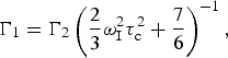 $${\rm \Gamma} _1 = {\rm \Gamma} _2 \left( {\displaystyle{2 \over 3}\omega _{\rm I}^2 \tau _{\rm c}^2 + \displaystyle{7 \over 6}} \right)^{ - 1}, $$
where τ c is in units of seconds and ω I is the 1H frequency in radians·s−1. To avoid having to use Eq. (64), one must use a long repetition delay (>4 × T 1,dia), especially for large and/or deuterated molecules (Iwahara et al. Reference Iwahara, Tang and Clore2007). Thus, under these circumstances, performing a single-time-point measurement offers no appreciable time savings over directly measuring the diamagnetic and paramagnetic transverse relaxation rates using multiple time points. Additionally, the requirement of a Lorentzian line shape for the single-time-point experiment limits data processing to the use of either an exponential window function or no window function at all for the direct 1H dimension. The use of broad Lorentzian lines can lead to increased peak overlap and can be especially problematic for larger proteins. This restriction does not apply to multiple-time-point experiments.
When conducting PRE experiments, the use of concentrations of paramagnetic protein that are too high can lead to PREs from random collisions between molecules, similar to solvent PREs. Relatively low concentrations (~0·3 mM) of sample can be used to avoid this undesirable effect, which can be detected by performing experiments with different concentrations, as the solvent PRE is directly proportional to the concentration of the paramagnetic species. For intramolecular PRE measurements, one can perform a control intermolecular experiment, where instead of having the paramagnetic spin label attached to the isotopically labeled species, one can make a sample with a mix of isotopically labeled (but not spin labeled) protein and paramagnetically tagged (but not isotopically labeled) protein. Any PRE measured in such an experiment would be from intermolecular effects.
Two-time-point PRE measurements can be performed within 1–2 days for a well-behaved small-medium-sized protein. For example, after 20 h each of measurement time for the paramagnetic and diamagnetic control, samples of 0·3 mM perdeuterated CaM–4Ca2+ measured using a two-time-point (20 ms delay) TROSY 2D 15N–1HN experiment at 600 MHz on a cryogenically cooled probe gave errors in Γ2 (calculated from S/N using Eq. (60)) of 1–2% for Γ2 ≈ 20 s−1 and 2–10% for Γ2 ≈ 50 s−1 (Anthis et al. Reference Anthis, Doucleff and Clore2011).
3.3 Data analysis
3.3.1 Fitting PRE data
Once PRE data are acquired, further analysis is needed to gain insight into macromolecular structure; this often involves back-calculating PRE values from atomic coordinates (either to test the agreement between experimental PRE values and a known structure or as part of a routine to calculate a new structure or ensemble from PRE data). Although it is tempting to interpret PREs directly as distances, this approach is problematic due to the flexibility of most common PRE spin labels (and the inherent flexibility of the macromolecules under study). As the PRE is a population-weighted 〈r −6〉 average of all states in exchange on a fast timescale, the PRE generally does not correspond to a single distance, and the contribution of a particular state can be very different than its fractional population (hence the utility of PRE for detecting minor states). Historically, this has made rigorous treatment of PRE data complicated, but computational advances have made such studies feasible.
One solution has been the incorporation of an ensemble average approach (Iwahara et al. Reference Iwahara, Schwieters and Clore2004b), which has been implemented in the macromolecular structure determination software package Xplor-NIH (Schwieters et al. Reference Schwieters, Kuszewski, Tjandra and Clore2003, Reference Schwieters, Kuszewski and Clore2006). Here, the paramagnetic group is represented by an ensemble of multiple conformers, and PRE values are the sum of the PREs for the individual conformers. Thus, using the ‘prePot’ pseudoenergy term in Xplor-NIH, one can refine directly against the experimental PRE values. Scripts and detailed instructions for these procedures are available online at http://spin.niddk.nih.gov/clore.
The first step in back-calculating PRE data in Xplor-NIH is the preparation of a suitable .pdb file, beginning with the in silico attachment of a spin label. The process is streamlined for common MTSL and EDTA tags. To prepare the .pdb file, one first changes the name of the residue where the tag is to be attached to ‘CYSP’ (for MTSL) or ‘CED’ (for EDTA). A script can then be run that fills in the missing atoms and regularizes their geometry (using the regularize module in Xplor-NIH). If the tag is not already in the Xplor-NIH library, one must generate parameter files and then attach the tag to the structure in silico. In order to use the SBMF PRE method, multiple conformations (at least 3) of the tag need to be generated.
Tag conformations are then refined by minimizing the target function for the PRE restraints, E PRE, defined as:
 $$E_{{\rm PRE}} = k_{{\rm PRE}} \sum\limits_i {w_i \left( {{\rm \Gamma} _2^{{\rm obs}} (i) - {\rm \Gamma} _2^{{\rm calc}} (i)} \right)^2}, $$
where k PRE is a force constant, w i is a weighting factor, Γ2obs(i) is the observed PRE, and Γ2calc(i) is the back-calculated PRE. The paramagnetic group is represented by an ensemble of N different conformers, while the remainder of the molecule is represented by a single structure. The individual members of the ensemble are treated independently and are allowed to overlap by excluding their interactions from the non-bonded energy term. This approach provides equal weights of 1/N to each member of the ensemble, but such an approach can account for uneven distributions if a larger N (>3) is used, since members of the ensemble can overlap in the simulation. The ensembleSimulation (Clore & Schwieters, Reference Clore and Schwieters2004b) module in Xplor-NIH (Schwieters et al. Reference Schwieters, Kuszewski, Tjandra and Clore2003, Reference Schwieters, Kuszewski and Clore2006) can also be used to explicitly specify or optimize different weights for each member of the ensemble (Deshmukh et al. Reference Deshmukh, Schwieters, Grishaev, Ghirlando, Baber and Clore2013).
To calculate the PRE value, the ensemble-averaged distance 〈r −6〉 for the distance between the observed nucleus (n) and the paramagnetic center (e) must be calculated as follows (Iwahara et al. Reference Iwahara, Schwieters and Clore2004b):
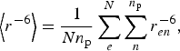 $$\left\langle {r^{ - 6}} \right\rangle = \displaystyle{1 \over {Nn_{\rm p}}} \sum\limits_e^N {\sum\limits_n^{n_{\rm p}} {r_{en}^{ - 6}}}, $$
where N is the number of ensembles used to represent the paramagnetic group and n p is the number of equivalent protons (e.g. 1 for NH or CH, 2 for NH2 or CH2, and 3 for CH3). Γ2 can then be directly calculated from the SB (Eq. (44)) or SBMF (Eq. (49)) equations; the SBMF equation is more accurate but requires additional computational time). Use of the SBMF equation requires the determination of an order parameter (S2) for each electron–nucleus vector, as defined by Eq. (51). In Xplor-NIH, order parameters are calculated on the fly from the ensemble of paramagnetic conformers, operating under the assumption that the fluctuations in the position of the measured nucleus are small compared with those of the paramagnetic center. Order parameters can be calculated using Eq. (52) together with the following equations (Iwahara et al. Reference Iwahara, Schwieters and Clore2004b):
 $${\bi S}_{{\rm PRE,angular}}^2 = \displaystyle{1 \over {N^2 n_{\rm p}^2}} \sum\limits_{e,d}^N {\sum\limits_{n.m}^{n_{\rm p}} {\left\{ {\displaystyle{3 \over 2}\left( {\displaystyle{{\vec r_{en} \bullet \vec r_{dm}} \over {r_{en} r_{dm}}}} \right)^2 - \displaystyle{1 \over 2}} \right\}}}, $$
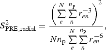 $${\bi S}_{{\rm PRE,radial}}^2 = \displaystyle{{\left( {\sum\limits_e^N {\sum\limits_n^{n_{\rm p}} {r_{en}^{ - 3}}}} \right)^2} \over {Nn_{\rm p} \sum\limits_e^N {\sum\limits_n^{n_{\rm p}} {r_{en}^{ - 6}}}}}, $$
where r en and r dm are vectors between the paramagnetic center (e, d) and the observed nucleus (n, m) in two different conformers. The values calculated in Eqs. (67) and (68) are the sum of contributions for each pair of conformers in the ensemble.
To fit the PRE values to the structure of a protein, a simulated annealing routine is performed with the protein molecule held rigid and the tags allowed to move to fit the data. Adjacent side chains can also be allowed to move to resolve steric overlap with the tag. At each step, Xplor-NIH will recalculate the order parameter for each PRE vector from the position of the different members of the tag ensemble. Fitting also requires the specification of correlation times, which can be explicitly provided or fit along with the tag positions in Xplor-NIH. If using the SB mode (i.e. Eq. (44)), only a single overall correlation time (τ c) is required, which depends on both the macromolecule rotational correlation time (τ r) and the electron spin relaxation time (τ s) (Eq. (45)). If τ s ≫ τ r (e.g. nitroxide spin labels (Bernini et al. Reference Bernini, Venditti, Spiga and Niccolai2009)), then the value of τ s can be ignored, and τ c is just simply τ r. However, if τ s is of the order of, or shorter than, τ r (e.g. paramagnetic metal ions), then the value of τ s must be taken into account. Under rigid SB assumptions, τ c can be calculated directly from the ratio of transverse and longitudinal PRE values (Iwahara et al. Reference Iwahara, Anderson, Murphy and Clore2003):
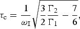 $$\tau _{\rm c} = \displaystyle{1 \over {\omega _{\rm I}}} \sqrt {\displaystyle{3 \over 2}\displaystyle{{{\rm \Gamma} _2} \over {{\rm \Gamma} _1}} - \displaystyle{7 \over 6}}, $$
where τ c is in units of seconds and ω I is the 1H frequency in rad·s−1. Equation (69) is only formally true for the SB approximation; however, even under SBMF conditions it offers a useful estimate of τ c (yielding maximum errors in the effective Γ2−1/6-calculated distance r of 4% for an order parameter of S2 = 0·5, with smaller errors for larger order parameters) (Iwahara et al. Reference Iwahara, Schwieters and Clore2004b). To avoid these errors, however, and in the absence of additional data, τ c can instead be optimized within a pre-defined range (Iwahara et al. Reference Iwahara, Schwieters and Clore2004b). If one is using the SBMF mode (i.e. Eq. (49)), which is more appropriate unless a rigid paramagnetic center is used, one must also take into account (in addition to τ c) the total correlation time τ t that incorporates τ r, τ s, and the internal correlation time for the PRE vector (τ i) (Eq. (G)). If τ r ≫ τ s and τ r ≫ τ i, one can use the approximation τ t ≈ 0, which assumes rapid motion of the PRE spin label. This in effect makes the order parameter S2 a scaling factor for the back-calculation of PRE data. This approximation does not hold true for shorter values of τ s. The prePot potential in Xplor-NIH also offers the option of optimizing τ c and/or τ t (or τ i) as part of the simulated annealing routine. Doing so then allows calculations to be performed with no prior knowledge of correlation times.
With these factors in place, Xplor-NIH can perform a simulated annealing calculation, refining directly against the experimental PREs, minimizing a target function including a pseudoenergy term calculated from the difference between back-calculated and experimental PRE values as well as terms to maintain proper geometry and avoid steric clashes. The goodness of fit of the PREs can be assessed by the Q-factor, which is analogous to the crystallographic R-factor and decreases with improved agreement between the observed (Γ2obs) and back-calculated (Γ2calc) rates (Iwahara et al. Reference Iwahara, Schwieters and Clore2004b):
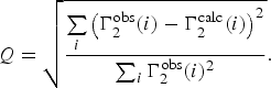 $$Q = \sqrt {\displaystyle{{\sum\limits_i {\left( {{\rm \Gamma} _2^{{\rm obs}} (i) - {\rm \Gamma} _2^{{\rm calc}} (i)} \right)^2}} \over {\sum\nolimits_i {{\rm \Gamma} _2^{{\rm obs}} (i)^2}}}}. $$
Alternatively, one can also use a reduced χ 2 statistic:
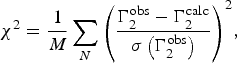 $$\chi ^2 = \displaystyle{1 \over M}\sum\limits_N {\left( {\displaystyle{{{\rm \Gamma} _2^{{\rm obs}} - {\rm \Gamma} _2^{{\rm calc}}} \over {\sigma \left( {{\rm \Gamma} _2^{{\rm obs}}} \right)}}} \right)} ^2, $$
where the degrees of freedom (M) are given by:
 $$M = N - 3C,$$
where N is the number of observed PREs and C the number of spin label conformers in the fitting ensemble (C is multiplied by three for the three translational degrees of freedom involved in fitting each nitroxide position). Other measures of the goodness of fit include the root mean-square-deviation (RMSD) between the observed and back-calculated PREs and the correlation coefficient from a linear regression fit of a scatter plot of the back-calculated versus observed PREs.
The representation of the paramagnetic label as an ensemble of multiple conformers is essential for fitting PRE data arising from flexible labels (e.g. MTSL). The use of a three-conformer ensemble improved the fit of PRE data from SRY/DNA complexes incorporating dT-EDTA-Mn2+ without overfitting the data – as indicated by a reduction in the free Q-factor calculated from data excluded from structure calculations and by the improvement of the fit of RDCs to the calculated coordinates (Iwahara et al. Reference Iwahara, Schwieters and Clore2004b). More rigid spin labels, however, do not require an ensemble representation. For example, it was demonstrated that, whereas multiple tag conformations were required to fit PRE data in CaM conjugated to MTSL, a single conformation was sufficient when CaM was conjugated to a pyridyl analog of MTSL (Fawzi et al. Reference Fawzi, Fleissner, Anthis, Kalai, Hideg, Hubbell and Clore2011a).
A scatter plot of the back-calculated PREs versus the experimental PREs is revealing of how good the fit is. However, for understanding the PREs in terms of structural features, a plot of PRE versus residue number (plotting both the back-calculated PREs and the experimental PREs) can be more informative. The key feature that indicates that a minor state might be present is the measurement of significantly higher PRE values than those back-calculated from the structure. However, before attempting to identify and characterize minor populations, one must first ensure that the experimental PRE data cannot be reasonably explained by a single structure. If these efforts fail to sufficiently explain the measured PREs, one can then attempt to calculate an ensemble of new structures to explain the data.
3.3.2 Ensemble simulated annealing calculations
If the PRE data collected on a system cannot be explained by known structures, the calculation of new structures or ensembles of structures may be necessary to satisfy the experimental data. The calculation of a molecular ensemble from average (in this case PRE) data is an inverse problem that is ill-posed and underdetermined for large ensembles and highly flexible systems. Thus, various approaches have been proposed (see below). Here, we describe the calculation of minor state structures using ensemble rigid body simulated annealing calculations using the ensembleSimulation module of Xplor-NIH (Clore & Schwieters, Reference Clore and Schwieters2004b).
In performing a rigid body refinement, the internal structure of all or part of a macromolecule is constrained to behave as a rigid body that is only able to translate and rotate as a cohesive unit (Clore, Reference Clore2000; Clore & Bewley, Reference Clore and Bewley2002). For example, CaM comprises two domains connected by a flexible linker; thus in PRE-driven ensemble simulated annealing calculations, each domain was treated as a rigid body, and residues in the linker were given full torsional degrees of freedom (Anthis et al. Reference Anthis, Doucleff and Clore2011). Side-chain residues at interfaces can also be allowed to move to prevent steric overlap. Rigid body refinement is appropriate only when the structure of the domains held rigid are not expected to change appreciably from the starting structure, a condition that can be validated by checking the agreement between experimentally measured RDCs and those back-calculated from the starting structure. The need for rigid body refinement arises from the sparse and long-range nature of the PRE, compared with conventional (NOE-based) NMR structural restraints. If sufficient additional data are available, full atomic structure calculations can be performed, although they will be computationally more expensive and the results may be ill defined compared with the results of a rigid-body refinement.
Additional points to consider are how many individual sets of PRE data (each from a molecule with a single paramagnetic tag) need to be included in the structure calculation and where the paramagnetic tags should be placed. Unless detailed information about the minor state(s) is known beforehand, the goal will be to have enough paramagnetic tags so that each position on the surface of the molecule would be within a distance that would generate a measurable PRE from at least one possible minor state conformation. Because some tag positions may disrupt the structure of the protein or have other undesirable effects, it is often necessary to test many more potential tag positions than might ultimately be required. In the case of CaM, which comprises two 8-kDa globular domains, we found that reproducible results required at least one tag on each of its two domains. Regardless of how many data sets are ultimately used, they can all be included in a single simulated annealing calculation.
Before calculating new ensemble structures to fit PRE data, the conformations of the spin labels must first be set using the fitting procedure described in Section 3.3.1, incorporating only the intramolecular or intradomain PRE data (i.e. data that comes primarily from the major state). These tag positions can then be maintained in the same conformations for the subsequent rigid body fitting. When performing simulated annealing calculations involving ensembles of minor states, one must determine an appropriate number of minor states and an appropriate population to fit the experimental data without overfitting. This can be accomplished by performing a grid search, i.e. performing multiple calculations while independently varying the number of minor states and the population attributed to each minor state. Increasing the number of minor states or the population attributed to each state should improve the fit (i.e. reduce the Q-factor) up to a certain threshold. The number N of minor states above which the Q-factor exhibits only marginal reduction is a good working value to use for calculations, as larger values of N will offer little improvement to the fit and will require proportionally more computational time. The minimum population and value of N needed to fit the data can be more rigorously determined by also calculating Q free (calculated the same as the Q-factor (Eq. (70)), but using a small percentage (e.g. 5%) excluded from the data set used for refinement). The value of N needed to fit the data varies from system to system, and a value under 10 is generally sufficient, even for fairly heterogeneous minor states. Likewise, the population above which the Q-factor exhibits only marginal reduction offers a good estimate of the true minor state population. For example, N = 8 was sufficient for CaM, in the presence or absence of calcium. A minor state of 10% was necessary to fit the calcium-loaded CaM data, but only 5% was needed for apo CaM (Anthis et al. Reference Anthis, Doucleff and Clore2011). New updates to Xplor-NIH allow users to directly fit the populations of ensemble members (Deshmukh et al. Reference Deshmukh, Schwieters, Grishaev, Ghirlando, Baber and Clore2013); however, this approach is applicable primarily to ensembles of more highly populated states because the populations of individual members of a minor state ensemble derived from PRE data can be ill-defined due to the dependence of the PRE on both the distance from the paramagnetic center and the population of each ensemble member.
Ensemble calculations can be computationally expensive, although the time required can be minimized through parallelization. The ensembleSimulation module in Xplor-NIH offers two types of parallelization (Clore & Schwieters, Reference Clore and Schwieters2004b), which can be used simultaneously. As with conventional structural determination in Xplor-NIH, individual ensembles can be calculated independently on different processors, as individual structures can. An additional level of parallelization can be added when using ensembleSimulation, as each member of the ensemble can also be calculated semi-independently on different processors.
The results of an ensemble simulated annealing calculation can be difficult to visualize, given that each ensemble could have tens of members, and the calculation might be repeated 100 or more times. Trying to visualize all individual ensemble members, especially at atomic resolution, can be both overwhelming and uninformative. Other visualization schemes, such as showing just the center of mass for each ensemble member, involve losing most detailed structural information. Reweighted atomic probability density maps, however, allow the consolidation of the full ensemble into a single representation, preserving many structural features and highlighting the major contributing members to the ensemble – a feature that may be lost in other representations (Schwieters & Clore, Reference Schwieters and Clore2002).
For visualizing NMR ensembles, instead of using an evenly weighted map, it is advantageous to calculate a probability density map that has been reweighted so that the maximum contribution of each atom is equal, allowing visualization of even the highly flexible regions of the molecule (Schwieters & Clore, Reference Schwieters and Clore2002). This is accomplished by defining the density at each point q as (Schwieters & Clore, Reference Schwieters and Clore2002):
 $$\rho _{{\rm reweight}} ({\bf q}{\rm )}{\bf =} \displaystyle{1 \over {N_s}} \sum\limits_{l = 1}^{N_{\rm a}} {w_l \sum\limits_{k = 1}^{N_{\rm s}} {\rho _a ({\bf q,q}_{kl} )}}, $$
where N s is the number of member structures in the ensemble, N a the number of atoms in each structure, qkl the position of atom l in each ensemble member, and w l a weighting factor. ρ a(q, qlk) is a quartic function, ranging from 0 to 1, that represents the electron density for each atom (Schwieters & Clore, Reference Schwieters and Clore2002):
 $$\rho _a ({\bf q,q}_{kl} ) = \left\{ {\matrix{ {\displaystyle{{105} \over {32\pi a^7}} \left( {d({\bf q,q}_{kl} )^2 - a^2} \right)} & {d({\bf q,q}_{kl} )\;{\rm \lt} \;a,} \cr 0 & {d({\bf q,q}_{kl} ) \ge a,} \cr}} \right.$$
where d(q, qlk) is the distance between point q and the center of the atom qkl, and a (set to 1 Å in Xplor-NIH) is defined so that ρ a(q, qlk) = 0·5 at d(q, qlk) = a × (1 − 1/√2)1/2. The weighting factor for each atom is defined as (Schwieters & Clore, Reference Schwieters and Clore2002):
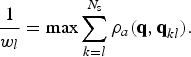 $$\displaystyle{1 \over {w_l}} = \max \sum\limits_{k = l}^{N_{\rm s}} {\rho _a ({\bf q,q}_{kl} )}. $$
These maps can be generated in Xplor-NIH and then visualized in a molecular graphics program such as VMD-Xplor (Schwieters & Clore, Reference Schwieters and Clore2001) or PyMOL (http://www.pymol.org). Showing this map at different contour levels gives a good indication of where the minor states are located, rather than looking at a large jumble of atoms, bonds, or ribbons. For the clearest results, it is often advantageous to generate multiple different maps in order to visualize the ensembles from multiple perspectives. For example, first, all structures could be aligned to rigid body A, and density maps could be calculated and visualized for rigid body B. Then, all structures could be aligned to rigid body B, and density maps could be calculated and visualized for rigid body A. The calculation and visualization of minor state ensembles allow structural insight into these important, transient species that have previously eluded structural characterization. The extent of insight possible will depend upon the heterogeneity of these ensembles, but if the structures are consistent from one ensemble to the next, it will be possible to analyze specific molecular contacts with a high degree of certainty. For larger or more heterogeneous ensembles, one might be restricted to identifying binding interfaces or other large-scale structural features. Regardless, the insights gained through these calculations shed substantial light on these elusive states and can provide a stepping stone for further biochemical study and manipulation of these minor states.
The PRE-driven ensemble calculation approach has been used to visualize transient interactions between the N-terminal domain of enzyme I (EIN) and the phosphocarrier protein HPr (Tang et al. Reference Tang, Iwahara and Clore2006, Reference Tang, Ghirlando and Clore2008a), between cytochrome c and cytochrome c peroxidase (Volkov et al. Reference Volkov, Worrall, Holtzmann and Ubbink2006, Reference Volkov, Ubbink and Van Nuland2010), between the N- and C-terminal domains of apo MBP (Tang et al. Reference Tang, Schwieters and Clore2007), between subunits of the HIV-1 protease precursor protein (Tang et al. Reference Tang, Ghirlando and Clore2008a), and between the N- and C-terminal domains of the calcium-sensing protein CaM (Anthis et al. Reference Anthis, Doucleff and Clore2011). Because these interdomain or intermolecular contacts only exist in a minor proportion (<10%) of the total population, they are invisible to conventional structural methods and could only be visualized by long-range paramagnetic NMR measurements. Thus, PRE can unlock fundamental insights into macromolecular-binding events, and many of these studies highlight the subtle interplay between induced fit and conformational selection in these binding events (Clore, Reference Clore2013).
3.4 Other approaches to treating PRE data
3.4.1 Maximum occurrence (MO), ensemble selection, and MD
In the previous sections, we discussed analyzing PRE data by fitting to known structures using simulated annealing calculations and characterizing minor states by using PRE-driven ensemble simulated annealing calculations. Various other methods are also available for calculating representative structural ensembles of a dynamic system (based on PRE data or on a variety of other NMR and non-NMR [e.g. SAXS] measurements), and these can broadly be placed in two categories (Fisher & Stultz, Reference Fisher and Stultz2011). The first category is the calculation of ensembles via simulated annealing calculations (Clore & Gronenborn, Reference Clore and Gronenborn1991; Clore & Schwieters, Reference Clore and Schwieters2004a, Reference Clore and Schwietersb, Reference Clore and Schwieters2006), as described above. Another broad class of methods involves first the generation of a large number of structures and then selection amongst these of the most appropriate ensemble to fit the experimental data. Examples include ENSEMBLE (Choy & Forman-Kay, Reference Choy and Forman-Kay2001), the ensemble optimization method (EOM) (Bernado et al. Reference Bernado, Mylonas, Petoukhov, Blackledge and Svergun2007), ASTEROIDS (Nodet et al. Reference Nodet, Salmon, Ozenne, Meier, Jensen and Blackledge2009), minimum ensemble selection (MES) (Pelikan et al. Reference Pelikan, Hura and Hammel2009), MO (Bertini et al. Reference Bertini, Giachetti, Luchinat, Parigi, Petoukhov, Pierattelli, Ravera and Svergun2010), and sparse ensemble selection (SES) (Berlin et al. Reference Berlin, Castaneda, Schneidman-Duhovny, Sali, Nava-Tudela and Fushman2013).
Some of these methods use molecular dynamics (MD) simulations to generate the initial set of individual conformers from which the final ensemble is selected. However, MD can be incorporated into the analysis of paramagnetic data in various ways. The simulated annealing approach discussed previously involves MD calculations with a simplified force field. Paramagnetic data and other NMR observables can also be incorporated directly into equilibrium MD simulations that also include explicit solvent and electrostatic force fields. Additionally, MD can be used to generate ensembles that can be analyzed for the fit of the experimental data. This approach was used to characterize CaM bound to the IQ-recognition motif from the voltage-gated calcium channel Cav1·2; the CaM/IQ complex had been crystallized in three different conformations, but in order to fit the PCS and paramagnetic RDC data on this complex in solution, all three crystal conformations plus four additional conformations calculated by MD had to be included (Russo et al. Reference Russo, Maestre-Martinez, Wolff, Becker and Griesinger2013).
Many different ensemble selection methods have been used for dynamic systems, but one that has been used extensively with paramagnetic data is the MO or maximum allowed probability (MAP) method described by Bertini and colleagues (Bertini et al. Reference Bertini, Gupta, Luchinat, Parigi, Peana, Sgheri and Yuan2007, Reference Bertini, Giachetti, Luchinat, Parigi, Petoukhov, Pierattelli, Ravera and Svergun2010, Reference Bertini, Ferella, Luchinat, Parigi, Petoukhov, Ravera, Rosato and Svergun2012a; Fragai et al. Reference Fragai, Luchinat, Parigi and Ravera2013) based on prior theoretical work (Gardner et al. Reference Gardner, Longinetti and Sgheri2005; Longinetti et al. Reference Longinetti, Luchinat, Parigi and Sgheri2006). This method has been used for paramagnetic PCS and RDC data (in combination with SAXS data) (Bertini et al. Reference Bertini, Giachetti, Luchinat, Parigi, Petoukhov, Pierattelli, Ravera and Svergun2010) as well as PRE data (Bertini et al. Reference Bertini, Luchinat, Nagulapalli, Parigi and Ravera2012b). A similar approach for PRE data has also been taken by Volkov et al. (Reference Volkov, Ubbink and Van Nuland2010). The MO approach involves first generating individual structures, as with other ensemble selection methods, and then determining a maximum population (‘occurrence’) that can be ascribed to each structure without violating the data. The result is a statistically rigorous view of the minor conformations observed by paramagnetic data, although without producing a tangible ensemble that can be used for further analysis.
The MO approach first requires generating a pool of random structures that comprehensively sample the rotational and translational conformational space accessible to the system. For a protein with two domains connected by a flexible linker (e.g. CaM), ~50 000 individual structures were required (Bertini et al. Reference Bertini, Giachetti, Luchinat, Parigi, Petoukhov, Pierattelli, Ravera and Svergun2010). For the transient interaction between two globular proteins (e.g. cytochrome c and cytochrome c peroxidase) ~1 000 000 individual structures were required to sample the interaction surface in 1-Å increments (Volkov et al. Reference Volkov, Ubbink and Van Nuland2010). A random structure generation protocol can be used to generate individual structures that fulfill basic criteria, such as lack of steric clashes between proteins or domains (Grishaev et al. Reference Grishaev, Anthis and Clore2012).
The MO procedure (Bertini et al. Reference Bertini, Ferella, Luchinat, Parigi, Petoukhov, Ravera, Rosato and Svergun2012a) is then performed for some subset of these (thousands to millions) individual structures. First, a structure is randomly selected and given a population. Then, an ensemble of a pre-determined size is selected to best fit the experimental data. A target function (e.g. Eq. (65)) is calculated, and this procedure is repeated for a range of different populations of the selected structure. The MO of this structure is defined as the maximum population that does not exceed the pre-set threshold value for the target function. The entire procedure is then repeated for a certain subset of the random structures available. The MO of each structure corresponds to an upper limit of the structure's population, but as the quantity of experimental data increases, the MO for each conformation should converge to its true population (Fragai et al. Reference Fragai, Luchinat, Parigi and Ravera2013). The different types of data that have been used in MO studies are highly complementary, being sensitive to either distance from a paramagnetic center (PRE), relative orientation (RDC), both of these (PCS), or overall molecular shape (SAXS). Additionally, the incorporation of multiple paramagnetic tag positions or the use of multiple paramagnetic metals with different g-tensors can also help to further refine the MO values (Fragai et al. Reference Fragai, Luchinat, Parigi and Ravera2013).
The MO method can be computationally expensive, although it lends itself well to parallelization. For this reason, the MaxOcc web portal (http://py-enmr.cerm.unifi.it/access/index/maxocc) has been set up to allow MO calculations on the e-NMR grid infrastructure (Bertini et al. Reference Bertini, Ferella, Luchinat, Parigi, Petoukhov, Ravera, Rosato and Svergun2012a). Another difficulty of MO analysis is finding a reasonable way to visualize the data. To simplify the presentation, the center of mass of each protein or domain can be represented as a dot, although this removes any orientational information. Instead of a dot, a set of axes can be used to represent the orientation of the molecule or domain, although information on interfaces and molecular contacts are still lacking. The MO can be indicated on such a representation through color coding. Also, unlike the ensemble simulated annealing approach, the MO approach does not generate concrete structural ensembles that can be used for further analysis.
The MO approach has been used extensively to characterize CaM (Bertini et al. Reference Bertini, Giachetti, Luchinat, Parigi, Petoukhov, Pierattelli, Ravera and Svergun2010, Reference Bertini, Luchinat, Nagulapalli, Parigi and Ravera2012b; Dasgupta et al. Reference Dasgupta, Hu, Keizers, Liu, Luchinat, Nagulapalli, Overhand, Parigi, Sgheri and Ubbink2011; Luchinat et al. Reference Luchinat, Nagulapalli, Parigi and Sgheri2012). These studies have incorporated PCS, RDC, PRE, and/or SAXS data from CaM, primarily using an N60D mutant that selectively binds lanthanide ions in one of the two N-terminal Ca2+-binding sites of CaM. These studies indicate that the two domains of CaM are capable of sampling a wide range of conformational space with respect to one another. Another study demonstrated that even when bound to a peptide from myelin basic protein, CaM was still highly dynamic (Nagulapalli et al. Reference Nagulapalli, Parigi, Yuan, Gsponer, Deraos, Bamm, Harauz, Matsoukas, De Planque, Gerothanassis, Babu, Luchinat and Tzakos2012). This flexible complex differed from the more rigid complex that Ca2+-loaded CaM forms with many peptide targets, but similar to that formed between apo CaM and a peptide from myosin light-chain kinase (Anthis et al. Reference Anthis, Doucleff and Clore2011). The MO approach was also used with SAXS, RDC, and PCS restraints to characterize matrix metalloproteinase-1 (MMP-1), revealing that MMP-1 adopts a more open structure in solution than that observed by X-ray crystallography (Cerofolini et al. Reference Cerofolini, Fields, Fragai, Geraldes, Luchinat, Parigi, Ravera, Svergun and Teixeira2013). A similar approach was also used to map the encounter complex between cytochrome c and cytochrome c peroxidase, although PRE-driven ensemble simulated annealing calculations were used to further refine the model of the encounter complex (Volkov et al. Reference Volkov, Ubbink and Van Nuland2010), demonstrating that the encounter complex adopts conformations nearby in space to the major species observed by X-ray crystallography (Volkov et al. Reference Volkov, Worrall, Holtzmann and Ubbink2006).
3.4.2 PRE studies on intrinsically disordered systems
PRE has proven to be a powerful method for studying unfolded and intrinsically disordered proteins, which, due to their dynamic nature, often defy characterization by other methods (Clore & Iwahara, Reference Clore and Iwahara2009; Clore et al. Reference Clore, Tang and Iwahara2007). Many studies on denatured systems have revealed evidence of residual structure in the unfolded state; examples include denatured staphylococcal nuclease (Gillespie & Shortle, Reference Gillespie and Shortle1997a, Reference Gillespie and Shortleb), the unfolded form of the N-terminal SH3 domain of drk (in slow-exchange equilibrium with the folded form) (Choy & Forman-Kay, Reference Choy and Forman-Kay2001; Marsh & Forman-Kay, Reference Marsh and Forman-Kay2009; Marsh et al. Reference Marsh, Neale, Jack, Choy, Lee, Crowhurst and Forman-Kay2007), acid-denatured apomyoglobin (Felitsky et al. Reference Felitsky, Lietzow, Dyson and Wright2008; Lietzow et al. Reference Lietzow, Jamin, Dyson and Wright2002; Silvestre-Ryan et al. Reference Silvestre-Ryan, Bertoncini, Fenwick, Esteban-Martin and Salvatella2013), denatured acyl coenzyme A-binding protein (Kristjansdottir et al. Reference Kristjansdottir, Lindorff-Larsen, Fieber, Dobson, Vendruscolo and Poulsen2005; Ozenne et al. Reference Ozenne, Noel, Heidarsson, Brander, Poulsen, Jensen, Kragelund, Blackledge and Danielsson2014), and the γ-subunit of cGMP phosphodiesterase (Song et al. Reference Song, Guo, Muradov, Artemyev, Ruoho and Markley2008). (However, PRE data on other systems have indicated that native-like populations constitute a very small or non-existent population in the disordered state (Cliff et al. Reference Cliff, Craven, Marston, Hounslow, Clarke and Waltho2009; Vise et al. Reference Vise, Baral, Stancik, Lowry and Daughdrill2007)). Studies on the intrinsically unstructured and aggregation-prone protein α-synuclein have revealed a more compact average hydrodynamic radius than expected for a truly random coil peptide as well as transient long-range interactions that appear to inhibit oligomerization and aggregation (Bertoncini et al. Reference Bertoncini, Jung, Fernandez, Hoyer, Griesinger, Jovin and Zweckstetter2005; Dedmon et al. Reference Dedmon, Lindorff-Larsen, Christodoulou, Vendruscolo and Dobson2005). PRE can also be used to identify interactions that could be productive for aggregation, as observed for the protein tau (Peterson et al. Reference Peterson, Zhou, Dahlquist and Lew2008).
Since disordered systems cannot be described by a single structure, ensemble approaches are usually appropriate (Fisher & Stultz, Reference Fisher and Stultz2011), including some of the methods described in Sections 3.3.2 and 3.4.1), although a very large and heterogeneous ensemble may be required to describe an unstructured system. Other alternative treatments of the data are also possible. For example, it has been demonstrated that the calculation of a single average structure can provide high-resolution information about residual molecular contacts in acid-unfolded apomyoglobin (Silvestre-Ryan et al. Reference Silvestre-Ryan, Bertoncini, Fenwick, Esteban-Martin and Salvatella2013), although it should be recognized that this does not provide an accurate representation of the reality in solution.
PRE data can be used to characterize flexible parts of otherwise more ordered systems. For example, recently the pH gating ability of loop 6 of the β-barrel outer membrane protein G was studied by PRE (Zhuang et al. Reference Zhuang, Chisholm, Chen and Tamm2013). PRE data have been used for studying systems involving structured domains linked by a flexible linker, including CaM (Anthis et al. Reference Anthis, Doucleff and Clore2011). The nature of the linker in this case was explored in further detail, as the extent of association between the two domains of CaM was determined by interdomain PRE measurements for linkers of varying length, and the results were fit to a simple random-coil model of the linker describing the effective concentration of the ends of the linker as a function of linker length (Anthis & Clore, Reference Anthis and Clore2013).
3.4.3 Solvent PRE
In addition to the measurement of PREs arising from a spin label or paramagnetic ion bound directly to a macromolecule (intramolecular PRE) or from a tag or ion bound to another macromolecule (intermolecular PRE), PREs arising from small co-solute molecules (solvent PRE) can also be measured. Such co-solute molecules include molecular oxygen (O2 (Hernandez et al. Reference Hernandez, Teng, Bryant and Lemaster2002; Sakakura et al. Reference Sakakura, Noba, Luchette, Shimada and Prosser2005)), nitroxides (e.g. TEMPOL (Fesik et al. Reference Fesik, Gemmecker, Olejniczak and Petros1991; Petros et al. Reference Petros, Mueller and Kopple1990)) and chelated metal ions (e.g. Gd-diethylenetriamine pentacetic acid-bismethylamide [Gd-DTPA-BMA or ‘Omniscan’] (Iwahara et al. Reference Iwahara, Zweckstetter and Clore2006; Pintacuda & Otting, Reference Pintacuda and Otting2002)). These particular co-solutes are neutrally charged, making them particularly appropriate as probes for solvent accessibility, although care must be taken with TEMPOL, which can preferentially interact with hydrophobic surfaces. Solvent PRE measurements can be used as structural restraints as a measure of solvent accessibility or proximity to the surface of a macromolecule, and they can also be used to detect intermolecular interactions (i.e. decreased PRE values near the interaction surface) (Iwahara et al. Reference Iwahara, Zweckstetter and Clore2006; Sakakura et al. Reference Sakakura, Noba, Luchette, Shimada and Prosser2005).
Analyzing solvent PRE data is complicated by the need to take into account the diffusion rates and correlation times of many co-solute molecules in addition to those of the macromolecule. Different theoretical frameworks have been proposed (Bernini et al. Reference Bernini, Venditti, Spiga and Niccolai2009; Clore & Iwahara, Reference Clore and Iwahara2009), including an inner-sphere model and an outer sphere model. In the inner-sphere model, the solvent PRE is assumed to arise from interactions between the paramagnetic protein and the macromolecular surface (Bloembergen, Reference Bloembergen1957; Solomon, Reference Solomon1955; Solomon & Bloembergen, Reference Solomon and Bloembergen1956), whereas in the outer-sphere model, the solvent PRE is assumed to arise from paramagnetic centers that behave as diffusive solvent molecules (Freed, Reference Freed1978; Hwang & Freed, Reference Hwang and Freed1975). Hwang and Freed have developed a theoretical framework to describe solvent PRE values by such an outer-sphere model, although due to its complexity it is difficult to apply to macromolecular structures.
Otting and LeMaster independently proposed an empirical method for back-calculating solvent PRE values from macromolecular structures (Hernandez et al. Reference Hernandez, Teng, Bryant and Lemaster2002; Pintacuda & Otting, Reference Pintacuda and Otting2002). The macromolecule is imbedded in a tightly spaced cubic lattice in silico, and the solvent PRE for a given nucleus in the macromolecule is the sum of the r −6 distances to each of the lattice points (excluding those that overlap with the macromolecule), weighted by a single empirical factor, a, which takes into account the concentration of the paramagnetic co-solute as well as its dynamics. This approach has been applied to solvent PRE data from O2 on 1H nuclei in rubredoxin (Hernandez et al. Reference Hernandez, Teng, Bryant and Lemaster2002), from Gd–DTPA–BMA on 1H nuclei in ubiquitin (Pintacuda & Otting, Reference Pintacuda and Otting2002), and from Gd–DTPA–BMA on 1H nuclei in specific and non-specific protein/DNA complexes (Iwahara et al. Reference Iwahara, Zweckstetter and Clore2006).
Some of these same solvent PRE co-solvents can be used in imaging studies as contrast agents. Conventionally, a non-toxic paramagnetic molecule (generally chelated Gd3+) is injected, and contrast is provided by the enhancement to longitudinal relaxation, measured as an increase in signal intensity where greater concentrations of the contrast agent are present (Caravan et al. Reference Caravan, Ellison, Mcmurry and Lauffer1999). Contrast agents have also been developed that take advantage of CEST and, more recently, paramagnetic contrast agents have been developed for paraCEST (chelated lanthanide ions, especially Eu3+) to generate even more dramatic chemical shift differences by hyperfine shifts for CEST imaging (Hancu et al. Reference Hancu, Dixon, Woods, Vinogradov, Sherry and Lenkinski2010; Vinogradov et al. Reference Vinogradov, Sherry and Lenkinski2013).
3.5 PRE in practice: application to CaM
CaM is the prototypical calcium-sensing protein in eukaryotes (Yamniuk & Vogel, Reference Yamniuk and Vogel2004), comprising two globular domains, each with two Ca2+-binding sites, connected by a short linker. CaM is a highly dynamic and pliable protein that binds to a wide range of target sequences, exerting different effects on various signaling pathways. A common mechanism is the release of target self-inhibition by binding to a regulatory peptide sequence and sequestering it to relieve inhibition. In such complexes, CaM forms a closed, compact structure, with its two domains in close proximity on opposite sides of a helical target peptide (Ikura et al. Reference Ikura, Clore, Gronenborn, Zhu, Klee and Bax1992; Meador et al. Reference Meador, Means and Quiocho1992) (Fig. 9). In the absence of target peptide, however, CaM forms a much more open structure. Although X-ray crystallography studies have consistently showed peptide-free Ca2+-loaded CaM (CaM-4Ca2+) in a highly extended ‘dumbbell’ conformation (Babu et al. Reference Babu, Sack, Greenhough, Bugg, Means and Cook1985), studies using a range of techniques, including NMR, have shown that the central linker is highly flexible (Barbato et al. Reference Barbato, Ikura, Kay, Pastor and Bax1992) and that in solution CaM forms structures intermediate between the fully extended and compact extremes (Trewhella, Reference Trewhella1992). However, there was previously no direct evidence for contacts between the two domains, and it was unclear whether compact states like those in the peptide-bound structure were accessible in solution, meaning that such compact states would have to occupy a low proportion of the total population.
Visualizing sparsely populated compact ‘dark’ states in Ca2+ activation of CaM. (a) Structures of CaM in various physiological states. Ca2+ ions are shown as red spheres, and spin-labeling sites S17C and A128C are indicated by yellow spheres. The flexible linker (residues 77–81) is shown in magenta. (b) Experimental PRE profiles for Ca2+-loaded CaM (with a spin label at S17C or A128C), in the presence or absence of peptide, are shown as circles (error bar, 1 s.d.). PREs too large (>80 s−1) to be accurately measured are plotted at the top of the charts. PRE profiles back-calculated from the structures of CaM–4Ca2+–peptide (red) and CaM–4Ca2+ (blue) are shown as solid lines. Only for the CaM–4Ca2+–peptide complex are the experimental interdomain PREs correctly predicted by the corresponding known X-ray structure. The bottom panel shows the resulting fits for a minor state population of 10% represented by an eight-member ensemble (magenta lines). (c) Dependence of the interdomain PRE Q-factor for S17C (blue) and A128C (green) as a function of minor state population for CaM–4Ca2+. (d) Modeling interdomain association in CaM–4Ca2+ (measured by PREs) as a local concentration effect. Empirical values of effective molarity (circles) were calculated from interdomain PRE data for CaM–4Ca2+ with different linker lengths (Anthis & Clore, Reference Anthis and Clore2013). These data were fit to an equation describing the theoretical values of the effective concentration of two points at the end of a random coil linker, where the interaction only occurs when the two points are separated by a defined distance. The best-fit line is shown in red (units of mM) and is a product of a pre-exponential factor (green) and exponential factor (blue). (e) The complex of CaM–4Ca2+ with an MLCK peptide is shown with CaM in cyan and the peptide in blue overlaid on the CaM–4Ca2+ dumbbell structure (green), best-fitted to either the N-terminal (left panel) or C-terminal (right panel) domains. The gray probability density maps represent 26 additional peptide-bound structures overlaid in the same manner. (f) Atomic probability density maps showing the conformational space sampled by the minor species ensemble for CaM–4Ca2+. The minor state atomic probability maps are derived from PRE-driven simulated annealing calculations using an eight-member ensemble with a population of 10%, and plotted at multiple contour levels ranging from 0·1 (transparent blue) to 0·5 (opaque red). The gray probability density maps, plotted at a single contour level of 0·1 of maximum, show the conformational space consistent with interdomain PRE values ≤2 s−1 and represent the major state ensemble characterized by no interdomain contacts and an occupancy of ~90%. In the left-hand panel, all ensemble members are best fitted to the N-terminal domain (dark green) and the probability density maps are shown for the C-terminal domain. In the right-hand panel, all ensembles are best-fitted to the C-terminal domain (dark green) and the probability density maps are shown for the N-terminal domain. Adapted from Anthis et al. (Anthis & Clore, Reference Anthis and Clore2013; Anthis et al. Reference Anthis, Doucleff and Clore2011).
In order to detect and characterize sparsely populated compact states in CaM, we collected PRE data on CaM with and without peptide (and with and without calcium; Anthis et al. Reference Anthis, Doucleff and Clore2011). Using paramagnetic nitroxide spin labels on each domain, we found that Ca2+-loaded peptide-bound CaM PRE data were fully consistent with a previously published crystal structure. However, even in the absence of peptide, significant interdomain PREs were observed that were inconsistent with the ‘dumbbell’ structure (which predicts no significant interdomain PREs) and which could not be explained by a combination of known structures. CaM also displayed interdomain PREs in the absence of Ca2+, although these PREs were much smaller than for CaM-Ca2+, and they were largely unaffected by the addition of target peptide. Because these PREs in peptide-free CaM could not be explained by pre-existing structures, we performed new calculations to characterize the minor states of CaM with close interdomain contacts.
PRE-driven simulated annealing calculations were performed in Xplor-NIH with the two domains of CaM treated as rigid bodies and the residues of the central linker given torsional degrees of freedom. The major species was represented by CaM in the ‘dumbbell’ conformation. Simulations were performed while varying both the size (N) and population of the minor state ensemble, and the goodness of fit was ascertained by a decrease in the Q-factor. Increasing the number N of molecules in the minor state improved the fit substantially up to N = 8, and then leveled off. Likewise, increasing the population improved the fit, but only to ~10% for CaM-4Ca2+ and ~5% for apo CaM. The improvement in fit can also be seen qualitatively in plots comparing the experimental PRE values with the values back-calculated from the ensembles (Fig. 9).
These simulations were performed using the SBMF mode of prePot in Xplor-NIH (Iwahara et al. Reference Iwahara, Schwieters and Clore2004b), with PRE order parameters calculated on the fly from a five-member ensemble of spin label conformers. This calculation was performed independently for each member of the minor state ensemble, because the motion of the spin label is much faster (ps) than the interdomain motion of CaM (ns). Each simulated annealing calculation was run 100 times, and the results were represented as reweighted atomic probability density maps (Schwieters & Clore, Reference Schwieters and Clore2002) (Fig. 9), which were calculated in Xplor-NIH and visualized using PyMOL (http://www.pymol.org).
From the probability density maps, it is clear that the two domains of CaM-4Ca2+ sample a wide range of conformational space, but they preferentially sample conformations similar to the compact peptide-bound state. However, such states are not accessible to apo CaM, even in the presence of target peptide. Thus, loading with Ca2+ primes CaM to bind to its peptide targets in part by making the compact peptide-bound conformations accessible even in the absence of target peptide. However, because these closed states occupied by CaM-4Ca2+ are similar, but not identical, to the conformations found in the closed peptide-bound form, it is clear that CaM target binding cannot proceed through a purely conformational selection mechanism, especially considering that the peptide-binding faces of the two domains of CaM would be inaccessible to the peptide in such a fully closed conformation. Thus, CaM target binding involves an interplay between induced fit and conformational selection, a phenomenon observed by PRE in other systems as well (Clore, Reference Clore2013; Tang et al. Reference Tang, Schwieters and Clore2007).
We found that in addition to this intramolecular interaction between the two domains of CaM, the N- and C-terminal domains of CaM form an intermolecular interaction that is similar in nature to the intramolecular interaction (as judged by the similarity between the intramolecular and intermolecular PREs) (Anthis et al. Reference Anthis, Doucleff and Clore2011). The nature of the attraction between the two domains is electrostatic, as increasing the ionic strength of the solution decreases the magnitude of interdomain PREs (Anthis et al. Reference Anthis, Doucleff and Clore2011). Further studies demonstrated that the formation of this intramolecular interdomain interaction is dependent upon the length of the flexible linker between the two domains, and the extent of interaction is directly proportional to the effective concentration of the two linkers (Fig. 9d). Because the two domains are constrained to be close in space by the linker, they interact much more tightly than in the absence of a linker, and the extent of interdomain association decreases as the linker is lengthened and the two domains become less constrained in space. However, decreasing the length of the linker from the wild type length also reduces interdomain association, as the two domains become highly constrained and are not able to form their interaction due to steric factors. We were able to explain these results with a simple model of two points at the ends of a random-coil linker, and further studies on the affinity of CaM for a target peptide showed that affinity is affected by linker length in the same manner as interdomain association (Anthis & Clore, Reference Anthis and Clore2013). Thus, the ability of CaM–4Ca2+ to form these compact structures in the absence of target peptide is directly related to its biological activity.
4. Characterizing large transient assemblies by DEST and lifetime line broadening
4.1 Theory
Characterizing large macromolecular assemblies by NMR is limited by the fact that as molecular weight increases, the rate of tumbling decreases, and the rate of transverse relaxation and therefore linewidth increases. Above a certain threshold, resonance linewidths become too broad and fall below the noise of the spectrum, making detection difficult or impossible. Additional difficulties arise if the large assembly is transient (and thus sparsely populated under equilibrium conditions) and if it is heterogeneous (e.g. intermediates in protein misfolding and aggregation). However, under conditions where a large ‘dark’ state is in equilibrium with a smaller visible species, DEST and lifetime line broadening (R llb) can be used to visualize states that are otherwise invisible to conventional structural biology (Fawzi et al. Reference Fawzi, Ying, Torchia and Clore2010b, Reference Fawzi, Ying, Ghirlando, Torchia and Clore2011b, Reference Fawzi, Ying, Torchia and Clore2012; Libich et al. Reference Libich, Fawzi, Ying and Clore2013). Whereas the characteristic that makes minor states visible by PRE is distance (i.e. close proximity between a spin label and an atom in the minor state), the property that makes dark states visible by DEST and R llb is size (one of the very factors that makes such states invisible in the first place). Thus, DEST and R llb are used to visualize molecules (i.e. small- to medium-sized proteins or peptides) in exchange with a much larger macromolecular assembly. As long as the visible species exchanges with the dark state on a timescale of ~500 μs–1 s, the footprint of the invisible species will be apparent as a broadening of the saturation profile and an increase in the apparent observed transverse relaxation rate (R 2obs) of the major species. To date, these methods have been used to study the aggregation of the Aβ peptide into protofibrils (Fawzi et al. Reference Fawzi, Ying, Torchia and Clore2010b, Reference Fawzi, Ying, Ghirlando, Torchia and Clore2011b, Reference Fawzi, Libich, Ying, Tugarinov and Clore2014) and its interaction with the chaperonin GroEL (Libich et al. Reference Libich, Fawzi, Ying and Clore2013).
4.1.1 Lifetime line broadening
Here, we consider a process, such as protein aggregation or the interaction of a protein with a larger macromolecular complex, where the system is in exchange between two states:
 $${\rm A}\; {\mathop{\rightleftharpoons}_{k_{\rm off}}^{k_{\rm on}^{\rm app}}} \; {\rm B,}$$
where state A is the visible species and state B is the invisible dark state. Exchange from states A to B is described by the pseudo-first-order rate constant k onapp, and exchange from states B to A is described by the first-order rate constant k off. Thus, at equilibrium:
 $$k_{{\rm on}}^{{\rm app}} [{\rm A}] = k_{{\rm off}} [{\rm B}].$$
The rate constant k onapp is a pseudo-first-order rate constant because although it describes a reaction that is first-order with respect to A, the actual reaction could be of higher order.
In such an exchanging system, the observed transverse relaxation rate (R 2obs) of state A can be enhanced by broadening due to differences in chemical shift between states A and B (R ex) and by broadening due to differences in transverse relaxation rate between the two states (lifetime line broadening, R llb). Overall, the enhancement (ΔR 2obs) to the transverse relaxation rate of state A is given by:
 $$R_2^{{\rm obs}} = R_{2,{\rm A}}^0 + {\rm \Delta} R_2^{{\rm obs}}, $$
where R 2,A0 is the intrinsic relaxation of state A in the absence of exchange. The relative contributions of R ex and R llb to ΔR 2obs depend on the exchange rate and on the magnitude of chemical shift difference (Δω = |ω A − ω B|) and transverse relaxation rate difference (ΔR 20 = R 2,B0 − R 2,A0) between the states (Fig. 5).
If the rate of transverse relaxation in state B (the ‘dark’ state; R 2,B0 = R 2dark) is very rapid (due a large size and therefore slow tumbling), then any transverse magnetization that is transferred from A to B will effectively be destroyed. If the exchange is slow on the transverse relaxation timescale (k ex ≪ ΔR 20), lifetime line broadening will be equal to the apparent first-order rate constant (R llb = k onapp). If, however, exchange is fast on the transverse relaxation timescale (k ex ≫ ΔR 20), R 2obs will be a population-weighted average of the two relaxation rates:
 $$R_2^{{\rm obs}} = p_{\rm A} R_{2,{\rm A}}^0 + p_{\rm B} R_{2,{\rm B}}^0 $$
(providing k ex ≪ 1/τ r, where τ r is the rotational correlation time) and R llb is given by:
 $$R_{{\rm llb}} = R_2^{{\rm obs}} - R_{2,{\rm A}}^{\rm 0} = p_{\rm B} {\rm \Delta} R_2^0. $$
For cases where the dark state B is very large and has a very rapid rate of transverse relaxation (e.g. large macromolecular assemblies and aggregated species), lifetime line broadening can only be measured in the slow exchange regime, unless p B is very small, because as R 2obs approaches values of ~100 s−1 or larger, it becomes difficult or impossible to measure. For smaller assemblies with more moderate R 2,B0, lifetime line broadening can be measured in the intermediate and fast exchange regimes as well.
If states A and B differ both in chemical shift and transverse relaxation rate, the manner by which R ex and R llb add up to ΔR 2obs depends on the value of the exchange rate (Fig. 5). For all exchange rates, the ΔR 2obs will be at least the magnitude of the greater of R ex and R llb, and ΔR 2obs will be at most the sum of the two. In the slow exchange regime (k ex ≪ ΔR 20 and k ex ≪ Δω), ΔR 2obs = R ex = R llb = k onapp. In the fast exchange regime (k ex ≫ ΔR 20 and k ex ≫ Δω), ΔR 2obs = R ex + R llb (and in the very fast regime, ΔR 2obs = R llb, as R ex approaches zero). In the intermediate exchange regime, ΔR 2obs will occupy a value intermediate between these two extremes (Fig. 5).
Values of ΔR 2obs, R ex, and R llb can be calculated by solving the McConnell equations (Eqs. (16)–(20)) and fitting the resulting time series to a single-exponential decay to derive a single apparent transverse relaxation rate (R 2obs). Subtracting R 2,A0 from R 2obs yields ΔR 2obs. The same procedure can be used to calculate R ex and R llb by setting ΔR 20 = 0 (to calculate R ex) and by setting Δω = 0 (to calculate R llb). Because R llb does not depend on chemical shift differences, it can be calculated by a simplified procedure only requiring the McConnell equations to be solved once. If all chemical shifts are set to zero (or if the −iΩ matrix in Eq. (16) is omitted), R llb can be calculated by the following expression:
 $$R_{{\rm llb}} = - \displaystyle{1 \over {T_R}} \ln \left( {\displaystyle{{M_{x,{\rm A}} (T_{\rm R} )} \over {M_{x,{\rm A}} (0)}}} \right) - R_{2,{\rm A}}^0, $$
where M x,A(0) is the initial value of x transverse magnetization on state A and M x,A(T R) is the magnetization at time T R (the specific value of T R is unimportant, but it can be set to an experimentally realistic value such as 0·1 s).
4.1.2 DEST
If a weak CW RF field is applied to a rapidly tumbling macromolecule, NMR signals at the same frequency as the CW RF radiation will be saturated, signals sufficiently far off resonance will be unaffected, and those near the RF frequency will be partially saturated. The width of this saturation profile increases with the transverse relaxation rate (R 2) of the nucleus and the strength of the CW RF field. For proteins or peptides that tumble rapidly and exhibit slow R 2 rates – and are thus visible by NMR – this profile is narrow. Large macromolecular complexes and assemblies (≥1 MDa), on the other hand, tumble slowly and exhibit large R 2 rates that make direct observation by solution NMR difficult or impossible due to the dramatically broadened linewidths; these large systems exhibit much broader saturation profiles. However, if such a dark state is in exchange with a visible species, it may be possible to indirectly study it via DEST, even if the dark state is also sparsely populated and/or has an amorphous or heterogeneous structure.
For a visible species in exchange with an invisible species, the overall R 2 rate for a nucleus signal will have contributions from both states. For the type of very large species that one might study by DEST (e.g. MW > 1 MDa), the transverse relaxation rate can become incredibly fast (e.g. >1000 s−1). Thus, transverse magnetization in the invisible species will quickly disappear, whereas more slowly relaxing longitudinal magnetization will remain intact. Thus, by just partially tilting the bulk magnetization of the sample toward the transverse plane (i.e. only partially saturating the magnetization) by the application of an off-resonance CW RF field, the overall signal will be attenuated but not destroyed. Under these conditions, nuclei in the invisible state will relax more quickly than nuclei in the visible state, but their magnetization will not disappear completely. Thus, due to the large difference in R 2 between the visible and invisible, the otherwise invisible large species can be detected by DEST (Fawzi et al. Reference Fawzi, Ying, Torchia and Clore2012).
The data from a DEST experiment can be modeled using a homogeneous form of the McConnell equations describing a system in equilibrium (Helgstrand et al. Reference Helgstrand, Hard and Allard2000). If the spins can be treated as isolated spins free of spin diffusion (e.g. 15N), the time dependence of the magnetization in this two-site exchanging system is given by (Helgstrand et al. Reference Helgstrand, Hard and Allard2000):
 $$\displaystyle{{\rm d} \over {{\rm d}t}}{\bf M =} -\left( {{\bf E + R + K + \Omega + S}} \right){\bf M}{\rm,} $$
where M is the vector describing the transverse magnetization of each state, R is the matrix describing the transverse relaxation rates of each state, K is the matrix describing the kinetic rates of exchange between each state, Ω is the matrix describing the chemical shift offset of the saturation pulse relative to the chemical shift of each state, S is the matrix describing the field strength of the saturation pulse, and E is the matrix describing the equilibrium magnetization. The exact equations will be dictated by the kinetic model describing the system, and here we consider a system in exchange between two states (Eq. (76)), where state A is the visible species and state B is the invisible dark state:
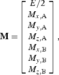 $${\bf M =} \left[ {\matrix{ {E/2} \cr {M_{x,{\rm A}}} \cr {M_{y,{\rm A}}} \cr {M_{z,{\rm A}}} \cr {M_{x,{\rm B}}} \cr {M_{y,{\rm B}}} \cr {M_{z,{\rm B}}} \cr}} \right],$$
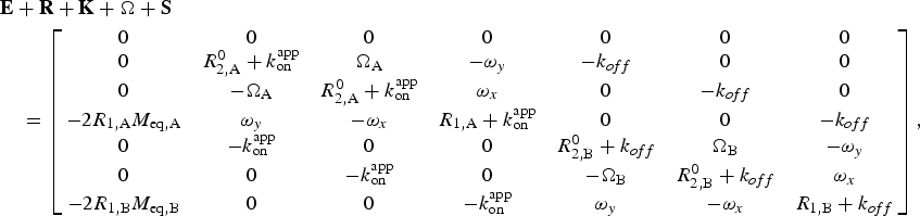 $$\eqalign{&{\bf E} + {\bf R} + {\bf K} + {\rm \Omega} + {\bf S} \cr &\quad = \left[ {\matrix{ 0 & 0 & 0 & 0 & 0 & 0 & 0 \cr 0 & {R_{2,{\rm A}}^0 + k_{{\rm on}}^{{\rm app}}} & {{\rm \Omega} _{\rm A}} & {-\omega _y} & {-k_{off}} & 0 & 0 \cr 0 & {-{\rm \Omega} _{\rm A}} & {R_{2,{\rm A}}^0 + k_{{\rm on}}^{{\rm app}}} & {\omega _x} & 0 & {-k_{off}} & 0 \cr {-2R_{1,{\rm A}} M_{{\rm eq,A}}} & {\omega _y} & {-\omega _x} & {R_{1,{\rm A}} + k_{{\rm on}}^{{\rm app}}} & 0 & 0 & {-k_{off}} \cr 0 & {-k_{{\rm on}}^{{\rm app}}} & 0 & 0 & {R_{2,{\rm B}}^0 + k_{off}} & {{\rm \Omega} _{\rm B}} & {-\omega _y} \cr 0 & 0 & {-k_{{\rm on}}^{{\rm app}}} & 0 & {-{\rm \Omega} _{\rm B}} & {R_{2,{\rm B}}^0 + k_{off}} & {\omega _x} \cr {-2R_{1,{\rm B}} M_{{\rm eq,B}}} & 0 & 0 & {-k_{{\rm on}}^{{\rm app}}} & {\omega _y} & {-\omega _x} & {R_{1,{\rm B}} + k_{off}} \cr}} \right],}$$
where E is unity, M is the magnetization of the A or B spin along each axis, and M eq is the equilibrium magnetization of each state. The longitudinal relaxation rates are given by R 1, and the intrinsic transverse relaxation rates (in the absence of exchange) are given by R 20. ω is the strength of the CW RF B 1 saturation field applied to each axis (ω [rad/s] = 2π × ν [Hz]), and ΩA and ΩB are the frequency offsets between the resonance frequency of the nucleus and the carrier frequency (in rad s−1). Equations describing three-state exchange (Fawzi et al. Reference Fawzi, Ying, Ghirlando, Torchia and Clore2011b) and two-state-exchange involving a multi-spin system (Fawzi et al. Reference Fawzi, Ying, Torchia and Clore2010b) have been described elsewhere.
A DEST (or CEST) profile can be calculated by solving Eq. (82) for a series of CW RF frequency offsets. For each offset, the signal intensity (I sat) is given by solving these equations for the time that the CW RF (ω x) field is applied. The DEST profile is plotted as I sat/I refversus carrier offset, where, I ref is the intensity in the absence of the saturation CW RF field, calculated as for I but with ω x = 0. Calculations are performed by starting with magnetization on the z-axis (M z,A[t = 0] = 1 × p A; all other components equal zero, including M z,B[t = 0], since the dark state magnetization would not survive the INEPT transfer if R 2,B0 is very large). Longitudinal magnetization decays to the equilibrium values of M eq,A and M eq,B. For 15N DEST, a value of M eq,A = M z,A[t = 0]/10 can be used, because γ H/γ N ≈ 10. A calculation is performed with magnetization beginning on +z, then a calculation is performed with magnetization beginning on −z (i.e. M z,A[t = 0] = 1 × p A, then M z,A[t = 0] = −1 × p A). The values from the second iteration (beginning on −z) are subtracted from the first (beginning on +z) because this difference yields a single-exponential curve that decays to zero in the absence of a saturation field). To properly simulate experimental data, the inhomogeneity of the B 1 saturation field should also be taken into account, which can be accomplished by repeating the calculations with a series of slightly different values of ω x (e.g. a Gaussian distribution about the desired value of ω x if the standard deviation of the field strength is known (Vallurupalli et al. Reference Vallurupalli, Bouvignies and Kay2012) or just ~10 fields strengths evenly spaced over a range of ω x ± 10% (Fawzi et al. Reference Fawzi, Libich, Ying, Tugarinov and Clore2014)).
A DEST (or CEST) profile can also be approximated by treating it as an off-resonance R 1ρ experiment (Palmer, Reference Palmer2014):
 $$I_{{\rm sat}} /I_{{\rm ref}} = \cos ^2 \theta \exp \,(-T_{{\rm sat}} R_{1\rho} ),$$
where T sat is the total saturation time, the angle θ is given by Eq. (34), and R 1ρ is given by Eq. (40) (as long as p A ≫ p B) for a DEST experiment (where R 2,A0 and R 2,B0 differ) or by simpler expressions (e.g. Eq. (39)) for CEST (as long as R 2,A0 = R 2,B0). Palmer has demonstrated good agreement between this analytical approximation, especially when Eq. (40) is used, compared to numerical solutions of the McConnell equations (Palmer, Reference Palmer2014).
4.2 Data acquisition
A system undergoing slow exchange between an NMR-visible species and a slowly tumbling invisible dark state can be well characterized by employing both lifetime line broadening measurements and DEST. These measurements have been performed on backbone amide 15N nuclei (Conicella & Fawzi, Reference Conicella and Fawzi2014; Fawzi et al. Reference Fawzi, Ying, Ghirlando, Torchia and Clore2011b, Reference Fawzi, Ying, Torchia and Clore2012; Libich et al. Reference Libich, Fawzi, Ying and Clore2013), methyl 13C nuclei (Fawzi et al. Reference Fawzi, Libich, Ying, Tugarinov and Clore2014) and 1HN nuclei (Fawzi et al. Reference Fawzi, Ying, Torchia and Clore2010b) (although the latter lack single-residue resolution due to rapid 1H–1H spin diffusion in the dark state). Measurements of both R llb and DEST for the same nucleus allow simultaneous fitting, which is necessary for precisely fitting the various parameters. For systems in the intermediate exchange regime, additional observables, including CPMG relaxation dispersion and exchange-induced chemical shifts, can also be useful (Libich et al. Reference Libich, Fawzi, Ying and Clore2013).
4.2.1 Measuring lifetime line broadening
Measuring lifetime line broadening requires being able to measure the R 2 values for the major state alone and in the presence of the dark state. To characterize the exchange of Aβ monomers with protofibrils, this was accomplished by acquiring data at both low concentrations of Aβ (no dark state present) and high concentrations (dark protofibrils present; Fawzi et al. Reference Fawzi, Ying, Torchia and Clore2010b, Reference Fawzi, Ying, Ghirlando, Torchia and Clore2011b, Reference Fawzi, Libich, Ying, Tugarinov and Clore2014). To characterize the interaction of Aβ with GroEL, data were measured in the absence and presence of GroEL (Libich et al. Reference Libich, Fawzi, Ying and Clore2013). Transverse relaxation can be measured using conventional pulse sequences (Cavanagh et al. Reference Cavanagh, Fairbrother, Palmer, Skelton and Rance2007) under conditions that eliminate any R ex contributions, using either a CPMG experiment with a large value of ν CP or a R 1ρ experiment with high spin-lock field strength. Under these conditions:
 $$R_{{\rm llb}} = {\rm \Delta} R_2^{{\rm obs}} = R_2^{{\rm vis + dark}} -R_2^{{\rm vis}}, $$
where R 2vis is R 2obs in the absence of the dark state and R 2vis+dark is in the presence of the dark state. R 2 is measured by varying, in an interleaved manner, the length of a delay during which the magnetization of the observed nucleus is on the xy-plane (generally at least ~8 different times, ranging from 0 × to ~1·3 × T 2), and fitting the intensity of each peak to an exponential decay function. Because it can be more straightforward to measure R llb, it is usually advisable to attempt to measure R llb before attempting to make more complex DEST measurements. Detection of lifetime broadening of R llb ≥ 1 s−1 is a strong indicator that DEST measurements will also be successful.
4.2.2 Acquiring DEST data
Most DEST experiments to date have been performed on 15N, which is advantageous because it provides one probe per residue, and it is not subject to spin diffusion – which complicates analysis of 1H DEST measurements – or spin–spin coupling – which complicates 13C measurements in universally labeled samples. The setup and analysis of a DEST experiment, which has recently been described in greater detail (Fawzi et al. Reference Fawzi, Ying, Torchia and Clore2012), will be summarized here.
15N DEST can be measured with a 2D HSQC-based experiment using the pulse sequence in Fig. 10. Pulse sequences for measuring DEST are available online at http://spin.niddk.nih.gov/clore/Software/software.html. A series of interleaved 2D experiments are performed, varying the frequency of the 15N CW saturation field. The optimal duration of the CW period is T 1 = 1/R 1. Experiments are performed at multiple saturation field strengths (e.g. 250 and 500 Hz) to assist in optimizing parameter values and discriminating between models. A reference experiment also needs to be performed with the saturation field turned off (i.e. strength of 0 Hz). The intensity of each peak is measured for each of these 2D experiments and plotted against the frequency offset of the CW saturation radiation. The spectrometer time required to acquire DEST data varies, but about 1 week was required to acquire the complete set of DEST and R 2 data on ~150 μM 15N-labeled Aβ using a cryogenically cooled probe (including the measurement of DEST at two different saturation field strengths; Fawzi et al. Reference Fawzi, Ying, Ghirlando, Torchia and Clore2011b).
Pulse sequence for the 2D 15N–DEST experiment. Full details are given in Fawzi et al. (Fawzi et al. Reference Fawzi, Ying, Ghirlando, Torchia and Clore2011b). During saturation experiments, the 15N CW saturation field is applied at a range of offset frequencies and at two different RF field strengths. During this period, a 180° 1H pulse train is applied (with 100 ms spacing between pulses) in order to eliminate longitudinal cross-correlated relaxation interference between the 15N–1H dipolar interaction and the 15N chemical shift anisotropy. Thus, for a saturation time of 0·9 s, for example, the saturation block would be repeated a total of n = 9 times. The optimal time for application of 15N saturation is the 15N–T 1 longitudinal relaxation time. In the reference experiment, the 15N saturation pulse is turned off (but the 180° 1H pulse train is still applied).
In order for DEST to be measured, the visible species, which gives rise to a 2D 1H–15N spectrum with well-resolved peaks and high S/N ratio, must be in exchange with a high-molecular-weight species (i.e. the ‘dark state’). Additionally, both k onapp and the rate constant for the transition of the dark state to the light state (k off) must be of the order of, or faster than, the R 1 rate of the nucleus undergoing saturation (e.g. ≥1 s−1 for backbone 15N). The lower limit on k off arises because longer residency periods in the dark state would cause too great a loss of signal before a significant number of transitions from the dark to visible state could be measured. The reason for the lower limit on k onapp is that, due to the extremely fast R 2 relaxation rate in the dark state, the creation of 15Nz magnetization must take place in the light state due to the inefficiency of the INEPT magnetization transfer in the dark state. Thus, it is also necessary to have a significant number of transitions from the light to the dark state within a time of T 1 = 1/R 1. Under conditions where R 2dark ≫ k off, there is also an upper limit of k onapp ≤ 100 s−1 as larger values will cause too great a loss of NMR signal and make measurement of DEST or R 2 difficult or impossible. Additionally, a minimum population of the dark state (~0·5% or higher) is required; leading to a rough lower limit of k onapp/k off > 0·005.
4.3 Data analysis
DEST and R llb data are fit simultaneously, as they offer complementary information on the same type of exchange processes. DEST data are analyzed by fitting the DEST profiles (intensity versus CW RF offset) to a kinetic model based on the McConnell equations (McConnell, Reference Mcconnell1958). The simplest model for fitting DEST data is a two-state model of exchange between a visible light state and an invisible dark state (Eqs. (82)–(84)). For a two-state model, the adjustable parameters are the global on- and off-rates (from which the relative visible and dark state populations are calculated), and R 2dark values (one for each observed nucleus). In addition to the DEST profiles and R llb values, R 2visible values need to be provided.
DEST and R llb data can be fit using the program DESTfit (Fawzi et al. Reference Fawzi, Ying, Torchia and Clore2012), which is available online at http://spin.niddk.nih.gov/clore/Software/software.html and has been described in detail previously (Fawzi et al. Reference Fawzi, Ying, Torchia and Clore2012). Once DEST and R llb data have been acquired and processed, the first step is to select the model to be used to fit the data. One should begin with a two-state model, only attempting fits with more complicated models if necessary. For a two-state model, the output includes the DEST profiles (one per nucleus) and plots of R llbversus residue and R 2darkversus residue; both experimental and back-calculated data are plotted together to help qualitatively judge the quality of the fit (Fig. 11) (Fawzi et al. Reference Fawzi, Ying, Torchia and Clore2012). By fitting DEST data to a kinetic model, one is able to gain great insight into the system under study, including the number of states and exchange events involved, and the kinetic parameters describing their exchange. Additionally, the fitted parameters of the dark state R 2 values provide a direct estimate of the size of the dark state as well as serve to locate the sites of interaction. Thus, DEST provides unique insight into systems where a visible state is in exchange with a larger invisible state on an intermediate-to-slow timescale.
Characterizing the exchange of Aβ peptides on the surface of large macromolecular assemblies by 15N–DEST and 15N lifetime line broadening (R llb). (a) Pseudo-two-state kinetic scheme for exchange of Aβ monomers with the surface of amyloid protofibrils. The ‘dark’ state comprises an ensemble of states where each residue can either be tethered or in direct contact with the surface of the oligomer. (b) 15N–DEST profiles for Glu3 and Leu17 at two different RF fields (170 Hz, orange; 350 Hz, blue). Experimental data are shown as circles, and lines represent the best fit for the simple two-state model (dashed) and the tethered/direct contact model (solid). (c) Residue-by-residue characterization of Aβ in exchange with the protofibril surface. The top panel shows 15N–R llb, with experimental data shown as black filled-in circles and calculated data shown as open circles for the simple two-state model (gray) or the tethered/direct contact model (blue). Also shown are profiles for the residue-specific partition coefficient K 3 (given by the ratio of direct-contact to tethered states) and 15N–R 2 values for the dark tethered states derived from the fits to the experimental R llb and DEST data. Data are shown for Aβ(1–40) (blue) and Aβ(1–42) (red). (d) Kinetic scheme for binding of Aβ(1–40) to GroEL. Values are listed for the populations of free (p A) and GroEL-bound (p B) Aβ in the presence of 20 μM (in subunits) GroEL. (e) 15N–DEST profiles for Glu3, Ala21, and Ile32 at two different RF fields (250 Hz, light; 500 Hz, dark). Experimental data are shown as circles, and lines represent the best fit from the simple two-state model. (f) Residue-by-residue characterization of Aβ in exchange with GroEL. The top panel shows 15N–R llb for 50 μM Aβ in the presence of 20 (circles) and 40 (diamonds) μM (in subunits) GroEL at spectrometer frequencies of 600 (blue) and 900 (red) MHz. Data are also shown for a control sample at 600 MHz (green) containing 50 μM Aβ40, 2·9 μM acid-denatured Rubisco, and 20 μM GroEL. The bottom panel shows back-calculated 15N–R llb values for GroEL-bound Aβ at 600 (blue) and 900 (red) MHz spectrometer frequencies. Adapted from Fawzi et al. (Reference Fawzi, Ying, Ghirlando, Torchia and Clore2011b) and Libich et al. (Reference Libich, Fawzi, Ying and Clore2013).
4.4 Combined approaches involving DEST
The information gained from DEST is complementary to other techniques used to characterize dark states on the same or different timescales (Fig. 1). Acquiring additional data using such complementary methods can help refine the values of fitting parameters and help characterize concurrent exchange events taking place on a timescale close to the faster exchange limits of DEST. For processes on the intermediate exchange regime, the measurement of relaxation dispersion and exchange-induced chemical shifts (ω ex) can be very helpful (Libich et al. Reference Libich, Fawzi, Ying and Clore2013). Although DEST and lifetime line broadening are optimal for describing exchange events on a timescale of ~1 ms–1 s, combining these observables with CPMG relaxation dispersion and exchange-induced chemical shifts enables study of exchange events of the order of 500 μs or faster.
ω ex is the observed difference in chemical shift of a nucleus in the presence of the dark state versus in the visible state alone (Eqs. (13) and (15)), and it is greater for larger differences in chemical shift between the two states (Δω) and for faster exchange rates (k ex). Extreme care must be taken when measuring ω ex because the values for ω ex in these types of systems can be very small (<1 Hz) (Libich et al. Reference Libich, Fawzi, Ying and Clore2013). Both ω ex (which is measured directly) and R ex (which can be measured indirectly by CPMG relaxation dispersion) arise from chemical shift differences between the visible and dark states, and they are most useful as probes of dynamics near k ex ≈ Δω. R ex has a maximum value at k ex = Δω. ω ex is most sensitive to k ex near k ex ≈ Δω, and it varies in value from zero in the slow exchange regime (k ex ≪ Δω) up to the population-weighted average chemical shift of the different states in the fast exchange regime (k ex ≫ Δω). Thus, CPMG relaxation dispersion and ω ex provide useful insight into exchange over timescales of ~500 μs–5 ms. A modification of the DESTfit program allows simultaneous fitting of CPMG relaxation dispersion and exchange-induced chemical shifts in addition to DEST and R llb data (Libich et al. Reference Libich, Fawzi, Ying and Clore2013).
4.5 DEST in practice: application to Aβ
A hallmark of Alzheimer's disease is the formation of extracellular plaques consisting of the Aβ peptide in fibrillar amyloid cross-β-strand structures (Goedert & Spillantini, Reference Goedert and Spillantini2006). However, smaller, more transient oligomers and protofibrillar forms of Aβ have more recently been linked with the presence of Alzheimer's disease, and intermediates in the Aβ aggregation pathway have been hypothesized to constitute the actual toxic species in Alzheimer's disease (Walsh & Selkoe, Reference Walsh and Selkoe2007). Despite much interest, little is known about the structures of these transient intermediates, how they form, and their role in Alzheimer's disease. These protofibrils are much too large (1·8–85 MDa) (Fawzi et al. Reference Fawzi, Ying, Ghirlando, Torchia and Clore2011b) to be directly characterized by conventional NMR and are not amenable to study by X-ray crystallography. Lower resolution methods, such as EM and AFM, offer some insight into their size and global structure, but provide little insight into their dynamic nature (Fawzi et al. Reference Fawzi, Ying, Ghirlando, Torchia and Clore2011b). DEST and R llb, however, have recently helped shed light on the details of these protofibrillar forms of Aβ (Fawzi et al. Reference Fawzi, Ying, Torchia and Clore2010b, Reference Fawzi, Ying, Ghirlando, Torchia and Clore2011b).
In the course of conducting NMR studies on transient interactions of Aβ, concentration-dependent 1H–R 2 values were observed that were largely uniform across the peptide. It was later shown that this was due to R llb – a loss of signal due to the exchange of the visible monomeric Aβ peptide with an invisible dark state on a slow (k ex ≪ R 2dark − R 2visible) timescale (Fawzi et al. Reference Fawzi, Ying, Torchia and Clore2010b). Fawzi et al. (Reference Fawzi, Ying, Torchia and Clore2010b) then showed that by applying 1H off-resonance saturation to Aβ displaying R llb, the broad saturation profile of the dark state became apparent in the overall saturation transfer profile of the visible species. This indicated that Aβ exchanges with a large species on a slow timescale, offering strong evidence that Aβ forms transient oligomeric intermediates (Fawzi et al. Reference Fawzi, Ying, Torchia and Clore2010b). These findings were further backed up by the visualization of such species by EM (Fawzi et al. Reference Fawzi, Ying, Torchia and Clore2010b). Although these initial studies were highly illuminating, quantitative analysis of 1H saturation transfer was difficult due to spin diffusion, limiting the conclusions to broader insights, and making atomic-resolution insights not possible. A major advance, however, was the development of 15N DEST, which removed the problem of spin diffusion, allowing atomic-resolution (or at least residue-resolution) insights to be gained. Using DEST, the authors were able to measure the kinetics of protofibril formation and show that two hydrophobic segments of the peptide (residues ~16–25 and ~28–37) were more tightly associated with the protofibrils (Fig. 11), and hence likely play a more central role in protofibril formation (Fawzi et al. Reference Fawzi, Ying, Ghirlando, Torchia and Clore2011b).
Lifetime broadening and DEST data were acquired on samples of Aβ(1–40) and Aβ(1–42) over a range of concentrations. The data could not be adequately fit with a simple two-state model, so more complex models had to be incorporated. The best fit was given by a pseudo-two-state model, whereby the Aβ peptide is in a two-state exchange between a visible state and a dark state, but in the dark state, each residue exists in either a direct contact or tethered state (i.e. two-site global exchange for the Aβ peptide, but three-site exchange on the level of each individual residue) (Fawzi et al. Reference Fawzi, Ying, Ghirlando, Torchia and Clore2011b). Using this kinetic model, the data were fit to a global overall rate of association with the protofibril surface (in either the tethered or direct-contact form), giving a concentration-dependent pseudo-first-order rate constant of k onapp = 3·0 ± 0·7 s−1 (for measurements on a sample comprising a total concentration of 270 μM Aβ(1–40) of which ~50% is in the protofibrillar form), consistent with the maximum R llb of 3·0 s−1 observed under these conditions. These data were also fit to global parameters for the dissociation rate constant from the dark state (k off = 51 ± 12 s−1) and the 15N-R 2 rate in the direct-contact dark state (15N-R 2contact = 18 800 ± 700 s−1) (Fawzi et al. Reference Fawzi, Ying, Ghirlando, Torchia and Clore2011b). Residue-specific parameters for the 15N-R 2 rate in the tethered state (R 2tethered) and the partition coefficient between the direct-contact and tethered states (K 3) were also fit. A larger value of K 3 indicates that the residue spends a higher fraction of time in the dark state in direct contact with the protofibrils surface rather than more loosely tethered (via other residues in direct contact with the protofibril surface), and a larger value of R 2tethered indicates a reduced average distance from the tethered residue to the site of direct contact. As a whole, these results provide an indirect picture of the otherwise invisible protofibrils of Aβ (Fawzi et al. Reference Fawzi, Ying, Ghirlando, Torchia and Clore2011b), showing that insight can be gained by solution NMR even on a system that is so large that it approaches the Redfield limit (Redfield, Reference Redfield1957) where T 2 ≫ τ r no longer holds true (for Aβ 1–40 protofibrils (Fawzi et al. Reference Fawzi, Ying, Ghirlando, Torchia and Clore2011b), 15N-T 2contact = 1/15N-R 2contact = 53 μs; τ r ≈ 40 μs for a spherical 85-MDa protein assembly at 10°C). Studies on Aβ(1–40), (1–42), and (1–43) have revealed broadly similar results, although faster association rates are observed for the longer peptides, consistent with their more rapid overall aggregation kinetics (Conicella & Fawzi, Reference Conicella and Fawzi2014; Fawzi et al. Reference Fawzi, Ying, Ghirlando, Torchia and Clore2011b). Additional lifetime line broadening and DEST studies were performed on the methyl 13C resonances of Aβ(1–40), revealing a strong correlation between backbone 15N-R llb and methyl 13C R llb (Fawzi et al. Reference Fawzi, Libich, Ying, Tugarinov and Clore2014). These data were best fit to a pseudo-two-state model with the same kinetic parameters as the 15N data. The best-fit value of 1/13C-R 2contact = 1230 ± 30 s−1 was significantly slower than 15N–R 2contact, consistent with the rapid rotation of methyl groups.
In another study, the authors characterized the transient interaction of the Aβ peptide with the chaperonin GroEL (Libich et al. Reference Libich, Fawzi, Ying and Clore2013). The chaperonins constitute a subclass of chaperone proteins, which facilitate protein folding in vivo (Horwich & Fenton, Reference Horwich and Fenton2009; Thirumalai & Lorimer, Reference Thirumalai and Lorimer2001). GroEL comprises two seven-member rings of 56-kDa subunits; substrates are known to bind to the inner cavity of GroEL, although the structures and dynamics of these complexes are largely unknown, due to the invisibility of the GroEL-associated substrate to conventional structural biology techniques. Although GroEL (780 kDa) is much smaller than the Aβ protofibrils previously characterized by DEST (up to 85 MDa), it is still large and slowly tumbling enough (R 2 > 1000 s−1) that the GroEL-associated Aβ is invisible to direct observation by NMR but also susceptible to off-resonance saturation at offsets greater than 1 kHz that could be transferred to the visible monomeric species (Libich et al. Reference Libich, Fawzi, Ying and Clore2013) (Fig. 11).
Experiments were performed on dilute (50 μM) Aβ in the absence or presence of GroEL at concentrations of 20 and 40 μM (in individual subunits). The addition of GroEL caused a large increase in 15N-R 2, which varied on a residue-by-residue basis from 1 to 23 s−1. This ΔR 2obs could be attributed almost fully to lifetime line broadening (versus chemical exchange broadening) because ΔR 2obs did not correlate with exchange-induced chemical shifts. DEST experiments were performed, and saturation transfer was observed in Aβ in the presence of GroEL (50% saturation at up to ~2 kHz off resonance for a saturation field strength of 500 Hz), although this effect was much smaller than seen with concentrated Aβ in exchange between monomeric and protofibrillar Aβ (Fawzi et al. Reference Fawzi, Ying, Ghirlando, Torchia and Clore2011b). CPMG relaxation dispersion experiments were also performed on Aβ, and dispersion was seen in the presence of GroEL, but not in its absence. These data were fit together (along with lifetime broadening data and exchange-induced chemical shifts) to a two-state exchange model characterizing the interaction of Aβ with GroEL, revealing both the kinetics of this process and the sites in Aβ most tightly associated with GroEL (Libich et al. Reference Libich, Fawzi, Ying and Clore2013). Based on these fits, in the presence of 20 μM GroEL (in subunits), 2·3% of Aβ peptides were bound to GroEL, and it associated with a pseudo-first-order rate constant of k onapp = 35 s−1 and dissociated with a first-order rate constant of k off = 1440 s−1 (Libich et al. Reference Libich, Fawzi, Ying and Clore2013). The degree of direct contact with GroEL on a residue-by-residue basis could be determined by the fitted R 2dark for each residue. The tightest asociation was observed for Aβ residues 16–21 and 30–36 (Libich et al. Reference Libich, Fawzi, Ying and Clore2013; Fig. 11), which are largely hydrophobic and correspond to consensus GroEL-binding sequences (Stan et al. Reference Stan, Brooks, Lorimer and Thirumalai2006). Additionally, 15N, 1HN, 13Cα, and 13Cβ chemical shifts of GroEL-bound Aβ were obtained through the fitting procedure, offering direct structural insight into the otherwise invisible dark bound state. Interestingly, the small magnitude of these chemical shifts (<1 ppm) and the fact that for all residues R 2dark ≪ 1000 s−1 (the value expected for a rigid 1H-15N bond in an assembly the size of GroEL), indicate that in the dark state the Aβ peptide remains predominately only partially associated with GroEL (i.e. only binding with one hydrophobic sequence at a time; Libich et al. Reference Libich, Fawzi, Ying and Clore2013).
5. Conclusion
Intermediate states in a range of biological processes, including protein folding, protein–protein interactions, enzyme catalysis, and protein aggregation, have defied high-resolution characterization. Various factors contribute to the invisibility of these states, including their transient nature, low population at equilibrium, and – in some cases, including protein aggregation – heterogeneity and large molecular weight, characteristics which are anathema to high-resolution structural biology by NMR, X-ray crystallography, or other methods. However, over recent years, developments in NMR methodology have opened these previously inaccessible states up to high-resolution characterization. These NMR methods are applicable over a wide range of timescales (Fig. 1) from the very fast (ps, ns, and μs) processes characterized by PRE (Clore & Iwahara, Reference Clore and Iwahara2009) and PCS (Bertini et al. Reference Bertini, Giachetti, Luchinat, Parigi, Petoukhov, Pierattelli, Ravera and Svergun2010) (e.g. protein–protein encounter complexes), to the intermediate (μs–ms) processes characterized by R 1ρ (Palmer & Massi, Reference Palmer and Massi2006) and CPMG relaxation dispersion (Korzhnev & Kay, Reference Korzhnev and Kay2008; Palmer et al. Reference Palmer, Kroenke and Loria2001) (e.g. protein folding and enzyme catalysis), intermediate-slow (μs–s) processes characterized by DEST (Fawzi et al. Reference Fawzi, Ying, Torchia and Clore2012) and lifetime line broadening (Fawzi et al. Reference Fawzi, Ying, Torchia and Clore2010b) (e.g. protein association aggregation), slow (ms) processes characterized by CEST (Vallurupalli et al. Reference Vallurupalli, Bouvignies and Kay2012) (protein folding and association), to the very slow (ms, s, and longer) processes characterized by hydrogen exchange (Englander et al. Reference Englander, Mayne and Krishna2007) (e.g. protein folding and aggregation).
The key to these methods is that they specifically and disproportionately amplify some aspect of the invisible state. Other methods, either using NMR (e.g. RDCs) or other techniques (e.g. SAXS/SANS) can provide information about minor states as part of the overall ensemble of structures being characterized. However, these average methods only report upon each structure proportionally to its population, limiting their utility for sparsely populated states. As long as the dark state is in chemical exchange with a visible species, though, and if one can take advantage of some unique aspect of the dark state – e.g. a shorter distance in a transient state than in the visible species (PRE) or a much larger molecular weight in the dark state than in the visible state (DEST or lifetime broadening) – it is possible to amplify the information from the dark state and make it visible. Underlying these methods is the enhancement of relaxation rates due to some aspect of the exchange with the invisible species, allowing the information from the invisible species to be viewed through the lens of the visible species.
An advantage of NMR is that from a single experiment, a great deal of information at the atomic or single-residue level can be acquired on an otherwise invisible state. Other methods for measuring distances, for example, such as FRET (Hillisch et al. Reference Hillisch, Lorenz and Diekmann2001) and DEER (Altenbach et al. Reference Altenbach, Kusnetzow, Ernst, Hofmann and Hubbell2008; Klug & Feix, Reference Klug and Feix2008) also magnify the effects of minor states, but only a single distance can be measured from each double fluorescent- or spin-labeled sample. However, a single NMR experiment offers hundreds to thousands of individual probes of distance and dynamics. Another advantage of NMR, though, which is true of any solution method, is that it can observe molecules under native or native-like conditions. Additionally, recent developments have also made it possible to perform some biomolecular NMR experiments on live cells (Dedmon et al. Reference Dedmon, Patel, Young and Pielak2002; Inomata et al. Reference Inomata, Ohno, Tochio, Isogai, Tenno, Nakase, Takeuchi, Futaki, Ito, Hiroaki and Shirakawa2009; Selenko et al. Reference Selenko, Serber, Gadea, Ruderman and Wagner2006), allowing measurements potentially in the most physiological environment possible. Thus, although much insight into the invisible states underlying biomolecular processes has already been gained from these NMR methods, the field may have only just begun to explore the potential of what it is capable.
6. Acknowledgements
We thank Nicolas Fawzi, Dennis Torchia, Vitali Tugarinov, Vincenzo Venditti and Jinfa Ying for useful discussions and other assistance. This work was supported by the Intramural Program of the NIH, NIDDK, and the Intramural AIDS Targeted Antiviral Program of the Office of the Director of the NIH (to G.M.C.).