1. Introduction
Turbulent entrainment is the transport of irrotational flow, across the turbulent/non- turbulent interface (TNTI), into the turbulent region (da Silva et al. Reference da Silva, Hunt, Eames and Westerweel2014a). It characterizes the mixing between the chaotic fluids and the ambient non-turbulent flow (Holzner & Lüthi Reference Holzner and Lüthi2011), as well as the enlargement of turbulence volume. Understanding this process is of great significance to various disciplines, including meteorology and oceanography (Mellado Reference Mellado2017). The entrainment has been detailed described from a global and a local perspective (van Reeuwijk, Vassilicos & Craske Reference van Reeuwijk, Vassilicos and Craske2021). Globally, the integral entrainment velocity is proportional to the typical velocity scale in the turbulent region, and is not related to viscosity (Turner Reference Turner1986; van Reeuwijk & Holzner Reference van Reeuwijk and Holzner2014; Cafiero & Vassilicos Reference Cafiero and Vassilicos2020). Locally, the instantaneous entrainment velocity is of Kolmogorov velocity scale  $v_{\eta }$, and is determined by the local vorticity production, diffusion and dissipation (Holzner & Lüthi Reference Holzner and Lüthi2011; Jahanbakhshi & Madnia Reference Jahanbakhshi and Madnia2016; Mistry et al. Reference Mistry, Philip, Dawson and Marusic2016); the total viscosity-independent entrainment flux is then achieved by the violent distorted TNTI surface (de Silva et al. Reference de Silva, Philip, Chauhan, Meneveau and Marusic2013; Mistry, Philip & Dawson Reference Mistry, Philip and Dawson2019; Kankanwadi & Buxton Reference Kankanwadi and Buxton2020).
Despite the detailed research available, how entrainment is modified by the turbulent coherent structures is still needed for practical applications, such as large-eddy simulation and the low-order models for flows (Neamtu-Halic et al. Reference Neamtu-Halic, Krug, Haller and Holzner2019; Cimarelli & Boga Reference Cimarelli and Boga2021). For small-scale structures, it has been observed that the  $\lambda$-scaled vortex close to TNTI will modulate its nearby entrainment rate in both numerical and experimental studies (da Silva et al. Reference da Silva, Hunt, Eames and Westerweel2014a; Mistry et al. Reference Mistry, Philip and Dawson2019; Neamtu-Halic et al. Reference Neamtu-Halic, Krug, Mollicone, Van Reeuwijk, Haller and Holzner2020), where
 $\lambda$ is the Taylor microscale. Statistically, the vital role of small-scale eddies could be reflected by the fact that the dominant length scale of TNTI normal velocity is of
 $\lambda$ (Balamurugan et al. Reference Balamurugan, Rodda, Philip and Mandal2020). Physically, the modulations have been underlined by Watanabe et al. (Reference Watanabe, Jaulino, Taveira, da Silva, Nagata and Sakai2017), where a small-scale eddy is artificially placed near the TNTI. This model can correctly predict statistical dynamics of entrained fluids, which indicates that details of entrainment movements are governed by small-scale eddies.
However, the entrainment is a multiscale process, which means that the large-scale motions – whose size is of the character length of flow – are also involved (Mistry, Dawson & Kerstein Reference Mistry, Dawson and Kerstein2018). The role of large-scale motions in turbulent entrainment is still controversial. It was once concluded that the large-scale motions dominate the entrainment (Brown & Roshko Reference Brown and Roshko1974; Dahm & Dimotakis Reference Dahm and Dimotakis1987). However, with the development of data resolution, it has also been reported that the contribution from large-scale motions are less than 10 % (Westerweel et al. Reference Westerweel, Fukushima, Pedersen and Hunt2005, Reference Westerweel, Fukushima, Pedersen and Hunt2009). More detailed multiscale analyses have been conducted by Philip et al. (Reference Philip, Meneveau, de Silva and Marusic2014) and Mistry et al. (Reference Mistry, Philip, Dawson and Marusic2016): by filtering the flow field with varying filter size  $\varDelta$, it is found that, although the tortuosity of TNTI and the instantaneous entrainment velocity vary in different
 $\varDelta$, the total entrainment flux is independent of
 $\varDelta$. More recently, the large-scale and small-scale velocity fields in a temporal jet were numerically separated and evolved independently (Cimarelli & Boga Reference Cimarelli and Boga2021). It was found that the entrainment is more violent in the large-scale velocity field, which again suggests the importance of large-scale motions. Are large-scale motions important to entrainment? How will they influence the entrainment and what are the underlying mechanisms? These questions remain to be answered.
This paper aims to shed new light on the questions above. Considering that the properties of large-scale motions depend strongly on flow configurations (Breda & Buxton Reference Breda and Buxton2019; Balamurugan et al. Reference Balamurugan, Rodda, Philip and Mandal2020; Neamtu-Halic et al. Reference Neamtu-Halic, Krug, Mollicone, Van Reeuwijk, Haller and Holzner2020), here we will focus on one type of flow: the turbulent boundary layers (TBLs). The large-scale motions of fluids concerned in the present work are the large-scale high/low-speed motions (H/L-SMs) which predominate the mass and energy transport in the outer region of TBLs (Adrian, Meinhart & Tomkins Reference Adrian, Meinhart and Tomkins2000; Dennis & Nickels Reference Dennis and Nickels2011; Lee, Sung & Zaki Reference Lee, Sung and Zaki2017). H-SMs contain large-scale coherence of positive streamwise velocity fluctuation  $u'$, statistically together with a downward flow; while L-SMs contain negative
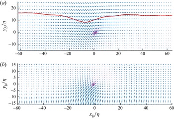
 $u'$ and statistically accompanied by an upwards flow (Lee et al. Reference Lee, Sung and Zaki2017). It will be shown that different large-scale motions will have different modulations on the engulfment and nibbling in TBLs. Furthermore, these effects are verified to be insensitive to the wall shape, thus being universal for TBLs. To the best of the authors’ knowledge, this is the first investigation of the wall-shape-independent large-scale modulations on the entrainment process.
In the TBL over a smooth wall, the occurrence of locations of large-scale motions is random. To illustrate the modulations of H/L-SMs intuitively, a special case is explored first: the TBL over ridge-type spanwise heterogeneous roughness. The location of H/L-SMs will be relatively locked due to the presence of heterogeneous roughness (Kevin et al. Reference Kevin, Monty, Bai, Pathikonda, Nugroho, Barros, Christensen and Hutchins2017; Medjnoun, Vanderwel & Ganapathisubramani Reference Medjnoun, Vanderwel and Ganapathisubramani2020; Wangsawijaya et al. Reference Wangsawijaya, Baidya, Chung, Marusic and Hutchins2020). After that, conclusions will be extended to more general cases, including the TBLs over smooth walls and homogeneous roughness. With the data and TNTI detection methods described in § 2, the TNTI over spanwise heterogeneity is first investigated in § 3. The acquired mechanisms are then extended to more general cases in § 4. Finally, the paper is summarized in § 5.
2. Experimental methods
2.1. Turbulent boundary layers data
TBLs over three kinds of wall shape are studied in this paper. The TBLs data over the heterogeneous and homogeneous roughness are acquired by the same sets of time-resolved two-dimensional particle image velocimetry (TR-2DPIV) and time-resolved stereoscopic particle image velocimetry (TR-SPIV) systems. The TBL over the smooth surface is acquired by direct numerical simulation (DNS).
The experiments are conducted at the low-speed water channel in Beihang University. The cylinder-shaped roughness elements for homogeneous roughness are formed by Lego bricks. The roughness elements are evenly spaced in the  $x$–
 $z$ plane. The spacing between two adjacent elements are approximately
 $0.15\delta$, where
 $\delta$ is the boundary layer thickness defined by the location of 99 % of the free stream velocity. The height of roughness elements is approximately
 $k/ \delta \approx 0.02$ while the diameter of elements is
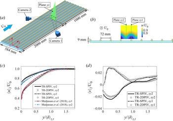
 $0.08\delta$. The spanwise heterogeneity is built by adding additional streamwise ridges on homogeneous roughness, as shown by the yellow ridges in figure 1(a). The spanwise spacing of adjacent ridges is selected to be
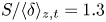 $S/\langle \delta \rangle _{z,t} = 1.3$ to induce intense secondary vortices (Wangsawijaya et al. Reference Wangsawijaya, Baidya, Chung, Marusic and Hutchins2020), where
 $\langle \rangle _{z,t}$ is taking the average along spanwise and time. The height of ridges is
 $h/\langle \delta \rangle _{z,t} = 0.17$ and the width is
 $W/\langle \delta \rangle _{z,t} = 0.14$. The Reynolds number based on the streamwise location
 $x$ of the field of view (FoV) is approximately
 $Re_x = 7.2 \times 10^5$. The Reynolds number
 $Re_{\lambda }$ based on the Taylor microscale
 $\lambda$ is 68, where
 \begin{equation} \lambda = \frac{1}{3}\left(\overline{u_I'^2}\left/\overline{\left(\frac{\partial u}{\partial x}\right)_I'^2}\right.+\overline{v_I'^2}\left/\overline{\left(\frac{\partial v} {\partial y}\right)_I'^2}\right.+\overline{w_I'^2}\left/\overline{\left(\frac{\partial w} {\partial z}'\right)_I^2}\right.\right), \end{equation}
and the subscript  $I$ is the value measured at TNTI. The streamwise, vertical and spanwise directions are denoted as
 $x$,
 $y$ and
 $z$, respectively. The corresponding velocity components are denoted as
 $u$,
 $v$ and
 $w$. The velocity fluctuations are denoted by the prime
 $'$.
(a) Stereoscopic view of TR-SPIV set-up. (b) Cross-section view of the TR-2DPIV set-up; the colour background illustrates the time-mean streamwise velocity. (c) Streamwise and (d) vertical velocity profiles from TR-SPIV and TR-2DPIV. The streamwise velocity profiles over a similar ridge-type heterogeneous roughness at higher Reynolds number ( $Re_x = 2\times 10^6$) (Medjnoun, Vanderwel & Ganapathisubramani Reference Medjnoun, Vanderwel and Ganapathisubramani2018) are also presented in panel (c) for reference.

The particle images for TR-SPIV are captured by two CMOS cameras (2048  $\times$ 2048 pixels) with Nikkor 85-mm tilt-shift lenses (figure 1a). The sampling frequency is 500 Hz. The entire FoV is focused by satisfying the Scheimpflug condition. The total FoV is approximately
 $2 S\times 1.8 S$ (
 $z \times y$). The average resolution is approximately 8 pixels per Kolmogorov length scale
 $\eta$ (using the value at
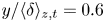 $y/\langle \delta \rangle _{z,t} =0.6$, according to Borrell & Jiménez Reference Borrell and Jiménez2016), which is high enough for TNTI-related research. The FoV plane in TR-SPIV is denoted as the plane
 $yz$ hereinafter.
TR-2DPIV is captured non-simultaneously at two  $x$–
 $y$ planes: the mid-plane of the ridge (denoted as plane
 $xy1$) and the mid-plane between two adjacent ridges (plane
 $xy2$), as shown in figure 1(b). As illustrated by the time-mean streamwise distribution, the two planes capture the centre planes of H/L-SMs, respectively. The PIV settings are identical to the TR-SPIV, and the resolution is also similar to TR-SPIV. The total FoV combined from two cameras is approximately
 $3.5 S\times 1.25 S$ (
 $x \times y$).
The velocity field is obtained with the multiple iterative Lucas–Kanade method with the 32  $\times$ 32 pixel window size and 75 % overlap at the last iteration (Pan et al. Reference Pan, Xue, Xu, Wang and Wei2015). The uncertainty of particle movement is 0.1 pixel. Since the averaged movement between two frames is approximately 10 pixels, the uncertainty of the obtained velocity is approximately 1 % in TR-2DPIV. The three velocity components in TR-SPIV are reconstructed from two cameras by the polynomial method (Soloff, Adrian & Liu Reference Soloff, Adrian and Liu1997). Self-calibration is applied before TR-SPIV calculation to eliminate the misalignment error (Wieneke Reference Wieneke2005). The velocity uncertainty in TR-SPIV is approximately 1.5 % considering the reconstruction (Van Doorne & Westerweel Reference Van Doorne and Westerweel2007). The velocity profiles obtained from TR-SPIV and TR-2DPIV at the same locations are presented in figure 1(c,d). The consistency of the profiles verifies the reliability of the present experiments. As a reference, the streamwise velocity profiles reported in Medjnoun et al. (Reference Medjnoun, Vanderwel and Ganapathisubramani2018) over a similar ridge-type spanwise heterogeneous roughness (
 $Re_x = 2 \times 10^6, S/\langle \delta \rangle _{z,t} \approx 0.8$) are also presented in figure 1(c). Qualitatively, the profiles coincide well, again proving the reliability of the experiments. The difference between the profiles at
 $xy1$ and
 $xy2$ in our experiments are larger, indicating that the influence of roughness on the flow field is greater. This could be attributed to the lower Reynolds number here (Medjnoun et al. Reference Medjnoun, Vanderwel and Ganapathisubramani2018).
The DNS data used in the present work are obtained from the open High-Reynolds-Numbers DNS Turbulent Boundary Layer Data from University Politecnica de Madrid. A zero pressure gradient turbulent boundary layer over a no-slip smooth wall is simulated. The corresponding simulation code originates from a high resolution code (Simens et al. Reference Simens, Jiménez, Hoyas and Mizuno2009) and is modified for high-Reynolds-number simulation (Borrell, Sillero & Jiménez Reference Borrell, Sillero and Jiménez2013). The statistics of flow properties are presented by Sillero, Jiménez & Moser (Reference Sillero, Jiménez and Moser2013, Reference Sillero, Jiménez and Moser2014), and are found to be consistent with previous experiments and simulations (De Graaff & Eaton Reference De Graaff and Eaton2000; Österlund et al. Reference Österlund, Johansson, Nagib and Hites2000; Jiménez et al. Reference Jiménez, Hoyas, Simens and Mizuno2010). The present data have been used for TNTI-related research (Borrell & Jiménez Reference Borrell and Jiménez2016); the results show that TNTI properties can be correctly captured. In our analysis, a  $3 \times 3 \times 3$ Gaussian filter is applied in calculating the enstrophy budget to eliminate the numerical noise.
2.2. Turbulent/non-turbulent interface detection method
For the DNS and TR-SPIV data, the enstrophy  $\omega ^2 = \omega _x^2+\omega _y^2+\omega _z^2$ is used to detect the TNTI with a selected threshold (Borrell & Jiménez Reference Borrell and Jiménez2016). In the TR-SPIV data, the streamwise deviation used for calculating
 $\omega ^2$ is obtained with Taylor's hypothesis. The threshold is chosen at the plateau in the curve of the TNTI mean height
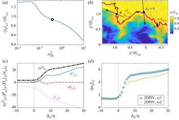
 $\langle y_I \rangle _{z,t}$ against the threshold, as shown in figure 2(a):
 $\langle y_I \rangle _{z,t}$ is relatively insensitive to the threshold at
 $\omega _{th}^2 \approx 0.4$, thus the threshold is selected here, as marked by the black open circle.
(a) Mean height of TNTI against enstrophy threshold  $\omega ^2_{th}$ from TR-SPIV data. (b) Local interface coordinate
 $\Delta _I$. The brown curve is the TNTI detected. (c) Conditional-averaged enstrophy
 $\langle \omega ^2 \rangle _I$, as well as enstrophy production
 $\langle P_{\omega } \rangle _I$, diffusion
 $\langle D_{\omega } \rangle _I$ and dissipation
 $\langle \epsilon _{\omega } \rangle _I$ from the TR-SPIV data. (d) Conditional-averaged spanwise vorticity magnitude from the TR-2DPIV data.

To verify that the TNTI captured here is reliable, the conditional-averaged enstrophy and its production  $P_{\omega }$, diffusion
 $D_{\omega }$ and dissipation
 $\epsilon _{\omega }$ are obtained along the TNTI local coordinate
 $\Delta _I$. Here,
 $\Delta _I$ is perpendicular to the local TNTI; it originates from the TNTI and points towards the turbulent region, as shown in figure 2(b). The quantity acquired by conditional average along
 $\Delta _I$ is denoted by
 $\langle \rangle _I$. To avoid local coordinates from crossing the interface multiple times, quantities at specified locations are excluded from the conditional average (Watanabe, Zhang & Nagata Reference Watanabe, Zhang and Nagata2018). For the coordinate crossing the TNTI at
 $|\Delta _I|<\varDelta _{thre}$, the total coordinate is excluded, as shown by coordinate A in figure 2(b). If the second cross-point is at
 $|\Delta _I|>\varDelta _{thre}$, then the region within a distance of
 $\varDelta _{thre}$ is excluded, as shown by the local coordinate B. The
 $\varDelta _{thre}$ is selected to be
 $8\eta$. It is checked that varying
 $\varDelta _{thre}$ from 2 to 15
 $\eta$ does not influence the conclusions in this paper. The conditional-averaged enstrophy and enstrophy budgets acquired from TR-SPIV are shown in figure 2(c). The results suggest that the detected TNTI is reliable. First, all the four quantities show significant variances in
 $\Delta _I = 0-O(10\eta )$, which imply that the thickness of TNTI is approximately
 $O(10\eta )$. This is consistent with previous research (Watanabe, da Silva & Nagata Reference Watanabe, da Silva and Nagata2020; Zecchetto & da Silva Reference Zecchetto and da Silva2021). Second, at
 $\Delta _I = 0$, it can be observed that
 $\langle D_{\omega }\rangle _I > \langle P_{\omega }\rangle _I$, indicating that the viscosity dominates the entrainment process across the TNTI, which also agrees with the results in the literature (Holzner et al. Reference Holzner, Lüthi, Tsinober and Kinzelbach2009). Third, by comparing
 $\langle D_{\omega }\rangle _I$ and
 $\langle P_{\omega }\rangle _I$, one can define the thickness of the laminar superlayer (
 $\langle D_{\omega }\rangle _I > \langle P_{\omega }\rangle _I$) and viscous sublayer (
 $\langle D_{\omega }\rangle _I < \langle P_{\omega }\rangle _I$). Here, the obtained thicknesses are approximately
 $4\eta$ and
 $11\eta$, respectively, which fall into the ranges reported by Silva, Zecchetto & da Silva (Reference Silva, Zecchetto and da Silva2018). Note that theoretically,
 $\langle \omega ^2 \rangle _I$ and
 $\langle \epsilon _{\omega } \rangle _I$ should be zero when
 $\Delta _I < 0$; the non-zero values here are due to the experimental noise.
For TR-2DPIV data without spanwise velocity, the magnitude of spanwise vorticity  $|\omega _z|$ is used for TNTI detection. As illustrated in previous studies (Watanabe et al. Reference Watanabe, Zhang and Nagata2018; Long, Wu & Wang Reference Long, Wu and Wang2021), the interfaces acquired from
 $|\omega _z|$ and
 $\omega ^2$ coincide well with each other. With the same threshold selection and conditional-average method, the
 $\langle |\omega _z| \rangle _I$ is presented in figure 2(d). For both planes, jumps of
 $\langle |\omega _z| \rangle _I$ can be clearly observed, indicating that the turbulent and non-turbulent regions are effectively separated.
3. Entrainment over spanwise heterogeneity
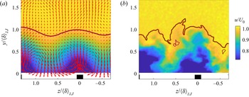
We first focus on the TBL over spanwise heterogeneity, since the locations of H/L-SMs are relatively locked. In the time-mean flow (figure 3a), L-SM is located in the vicinity of a ridge ( $z/\langle \delta \rangle _{z,t} \approx 0$), while H-SMs is between two ridges (
 $z/\langle \delta \rangle _{z,t}\approx \pm 0.65$). Although the large-scale motions meander in instantaneous flow (figure 3b), their spanwise movements are still small compared to
 $\delta$. The flow patterns are similar with previous works (Kevin et al. Reference Kevin, Monty, Bai, Pathikonda, Nugroho, Barros, Christensen and Hutchins2017; Medjnoun et al. Reference Medjnoun, Vanderwel and Ganapathisubramani2020).
(a) Time-mean and (b) instantaneous velocity field over the spanwise heterogeneity. Brown curves, TNTI (thick) and the non-turbulent bubbles (thin); red arrows, in-plane velocity.

To characterize the modulation of H/L-SMs on the entrainment, two processes of entrainment are defined following Jahanbakhshi & Madnia (Reference Jahanbakhshi and Madnia2016). The irrotational fluids become turbulent by either enstrophy propagation at the TNTI or by being pulled into the turbulent region and forming non-turbulent ‘bubbles’ inside the turbulent region. In this paper, the former is defined as nibbling while the latter as engulfment (Kevin et al. Reference Kevin, Monty, Bai, Pathikonda, Nugroho, Barros, Christensen and Hutchins2017; Jahanbakhshi & Madnia Reference Jahanbakhshi and Madnia2016).
Quantitatively, nibbling flux per wall unit  $F_n$ is the integration of the entrainment velocity
 $v_n$ along the TNTI (Holzner & Lüthi Reference Holzner and Lüthi2011), i.e.
 \begin{equation} F_n ={-}\frac{1}{L} \int_{TNTI} v_n \,{\rm d}s, \end{equation}
where  ${\rm d}s$ is the element of length along the TNTI and
 $L$ is the corresponding wall length. The minus in (3.1) is to keep the flux towards the turbulent region positive.
As for the engulfment flux  $F_e$, it is not easy to be obtained in an Euler frame. Here, it is assumed that the bubble close to the TNTI originates from the engulfment, and the engulfed bubbles are pulled into the turbulent region in a certain time interval
 $\Delta t_b$. Now,
 $F_e$ is then estimated as the total area of bubbles close to the TNTI divided by
 $\Delta t_b$ (Jahanbakhshi & Madnia Reference Jahanbakhshi and Madnia2016):
 \begin{equation} F_e = \frac{1}{L}\sum_{\varDelta_{B-I} < \varDelta_{thre}}S_b/\Delta t_b, \end{equation}
where  $\varDelta_{B-I}$ is the distance from the centroid of the bubble to the TNTI and
 $S_b$ is the area of the bubble. In § 3.2, the reasonability the assumption and the choice of
 $\varDelta _{thre}$ and
 $\Delta t_b$ will be shown.
To avoid ambiguity, it should be noted that the definitions of both engulfment and nibbling may be different in various works. In the multiscale analysis by Philip et al. (Reference Philip, Meneveau, de Silva and Marusic2014) and Mistry et al. (Reference Mistry, Philip, Dawson and Marusic2016), the engulfment and nibbling are defined as the entrainment related with large- and small-scale structures. However, in the present work, both processes could involve multiscale motions; the modulations of large-scale motions on entrainment will be investigated by checking the variance of engulfment and nibbling fluxes near the H/L-SMs.
3.1. TNTI geometry properties
From the definition, it can be noticed that the entrainment magnitude is highly related with the geometry properties of TNTI. So in this subsection, two of the key geometrical properties are discussed: the probability distribution function (p.d.f.) of the TNTI height  $y_I$ and the tortuosity of the interface.
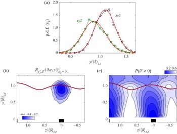
Figure 4(a) illustrates the p.d.f.s of  $y_I$. The p.d.f.s show negative (
 $-0.14$) and positive (0.56) skewness values at the planes
 $xy1$ and
 $xy2$, respectively, which differ from the Gaussian distribution with negligible skewness reported in canonical TBLs over smooth walls (Watanabe et al. Reference Watanabe, Zhang and Nagata2018; Wu et al. Reference Wu, Wang, Cui and Pan2020). The skewness demonstrates that the H-SM tends to draw the non-turbulent flows deep into the turbulent region, indicating the engulfment rate could be larger above the H-SM. Moreover, the standard deviation of
 $y_I$ in the plane
 $xy1$ (
 $0.15 \langle \delta \rangle _{z,t}$) is smaller than that in the plane
 $xy2$ (
 $0.19 \langle \delta \rangle _{z,t}$); and the magnitude of skewness is also smaller in the plane
 $xy1$ than that in
 $xy2$; these facts mean that the TNTI could be more distorted over the H-SM, thus benefiting the nibbling. Since these two planes are at the centre of H/L-SMs, it is natural to expect that the skewness is attributed to velocity fluctuations. To verify that, we calculate the correlation coefficient between the fluctuation of TNTI height
 $y_I'=y_I-\langle y_I \rangle _t$ and the streamwise velocity fluctuation
 $\tilde {u}'=u-\langle u \rangle _{z,t}$. At a specified spanwise location
 $z_0$,
 $y_I'(t)|_{z_0}$ is correlated with the velocity fluctuation signal at surrounded coordinate points
 $(z_0+\Delta z,y)$. The coefficient is defined as
 \begin{equation}
R_{y_I',\tilde{u}'}(\Delta z,y)|_{z_0} = \frac{\langle y_I'
(t)|_{z_0} \tilde{u}'(t)|_{z_0+\Delta z,y}
\rangle_t}{\sigma(y_I'
(t)|_{z_0})\sigma(\tilde{u}'(t)|_{z_0+\Delta z,y})},
\end{equation}
where  $\sigma$ is the standard deviation and
 $z_0$ is the reference spanwise location. Figure 4(b) shows the distribution of
 $R_{y_I',\tilde {u}'}(\Delta z,y)|_{z_0=0}$; a large area of negative value can be noticed below the TNTI. The negative coefficient indicates that the local TNTI tends to elevate when
 $\tilde {u}'<0$ and sink when
 $\tilde {u}'>0$. At the plane
 $xy1$,
 $\tilde {u}'$ is more likely to be negative (as shown in figure 4c) due to the presence of L-SM. As a result, the p.d.f. at the plane
 $xy1$ skews negatively. Similarly, the positive skewness of the p.d.f. at the plane
 $xy3$ is attributed to the presence of H-SM.
(a) P.d.f. of  $y_I$ at the two locations; the red curves are the Gaussian distributions. (b) Distribution of correlation coefficient between
 $y_I'$ and
 $\tilde {u}'$; the reference location is at
 $z_0=0$. (c) Probability of
 $\tilde {u}'>0$. The brown curve is the time-mean TNTI location.

The tortuosity is defined as the area of TNTI per projected area on the wall (in 3-D) or the length of TNTI per streamwise distance  $L_I/L_x$ (in 2-D) (Breda & Buxton Reference Breda and Buxton2019; Kankanwadi & Buxton Reference Kankanwadi and Buxton2020). From (3.1), it can be seen that larger tortuosity could result in larger nibbling: if we assume that
 $v_n$ is constant, then (3.1) writes as
 $v_n\times L_I/L_x$. The maximum likelihood tortuosity obtained at the planes
 $xy1$ and
 $xy2$ are
 $2.03 \pm 0.01$ and
 $2.15 \pm 0.01$ (95 % confidence interval, estimated from lognormal distribution), respectively. The TNTI above L-SMs owns larger tortuosity, which is consistent with the observation by Medjnoun et al. (Reference Medjnoun, Vanderwel and Ganapathisubramani2018): the flow beneath the TNTI in the L-SM region was reported to be more chaotic, thus resulting in a smaller intermittency.
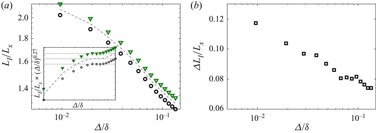
To explore the scales of structures which lead to the different tortuosity, the vorticity field is further filtered with a 2D box filter, then the TNTI is detected in the filtered field with the same detection threshold in the original enstrophy field. Figure 5(a) shows the tortuosity of TNTI against the box filter size  $\varDelta$. In both planes, the tortuosities decrease with the increase of
 $\varDelta$, since more small-scale structures are smoothed out. It could be noticed that a constant descent slope region (
 $-0.27$) emerges at approximately
 $0.05 \delta <\varDelta < 0.1\delta$ for both planes, as denoted by the plateau regions in the inset of figure 5(a). The constant slope is attributed to the fractal properties of TNTI (de Silva et al. Reference de Silva, Philip, Chauhan, Meneveau and Marusic2013). In the L-SM and H-SM regions, the slope stays the same, which shows that the two regions share the same fractal dimension and implies that large-scale motions do not influence TNTI's fractal dimension. The fractal dimension acquired here (
 $2.27 = 2+0.27$) is slightly smaller than the results
 $(7/3)$ in high-Reynolds-number TBLs (de Silva et al. Reference de Silva, Philip, Chauhan, Meneveau and Marusic2013), which could be attributed to the insufficient scale separation in the present Reynolds number (Mistry et al. Reference Mistry, Dawson and Kerstein2018; Wu et al. Reference Wu, Wang, Cui and Pan2020).
(a) Tortuosity of TNTI  $L_I/L_x$ against the box filter size
 $\varDelta/\delta$; open black circle, the plane
 $xy1$ (L-SM); open green triangle, the plane
 $xy2$ (H-SM); dash curve, the baseline case without being conditional averaged. The inset shows the tortuosity multiplied by
 $(\varDelta /\delta )^{0.27}$ to illustrate the constant slope region. (b) Difference between the tortuosity of TNTI at two planes against the box filter size.

Figure 5(b) further shows the difference of tortuosity between the two planes  $\Delta L_I/L_x$. The variation could be divided into three segments. The difference first declines in small-scale regions (
 $\varDelta < 0.05\delta$, i.e.
 $\varDelta \sim O(\lambda )$). This could be attributed to the formation of interface wrinkles when ‘bubbles’ are engulfed, as shown in Jahanbakhshi (Reference Jahanbakhshi2021); and the occurrence of more bubbles induces more wrinkles above the H-SMs. An evidence is that the difference of tortuosity will decline if increasing the TNTI detection threshold and connecting the bubbles with the TNTI, as will be shown in figure 17(c). Then,
 $\Delta L_I/L_x$ stays unchanged in the range of
 $0.05\delta <\varDelta < 0.1\delta$, indicating the middle-scale structures are not related to the difference. Finally, the difference further decreases when
 $\varDelta > 0.1\delta$, showing that the large-scale structures themselves will directly affect the tortuosity. This could be explained by the observations in Lee et al. (Reference Lee, Sung and Zaki2017). They found that the depth of the TNTI valley above H-SMs is larger than the height of the TNTI crest above L-SMs. This will also be seen in figure 15(a,b). The larger deformation indicates the TNTIs are elongated more violently. As a result, the TNTIs above H-SMs are distorted more violently.
3.2. Entrainment properties: engulfment flux
The geometrical properties show the modulation effects indirectly; now direct comparisons are made by calculating the entrainment fluxes.
To calculate the flux of engulfment, the bubbles are detected as the low enstrophy region in the turbulent flow. The detection threshold is the same as the TNTI detection threshold. Bubbles with area smaller than  $3\times 3$ data points (approximately
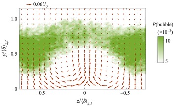
 $3\eta \times 3\eta$ in the physical world) are ignored to avoid the disturbance of noise. The effectiveness of bubble detection is checked in Appendix B. An instantaneous pattern of the bubbles is presented in figure 3(b). Two bubbles can be observed in the instantaneous H-LMs, which suggests the preference of bubbles in the H-LM regions. This is verified in figure 6, which shows the variance of the bubble occurrence probability
 $P(bubble)$ in the plane
 $yz$. As is apparent,
 $P(bubble)$ is much larger in the vicinity of H-SMs (
 $z/\langle \delta \rangle _{z,t} \approx \pm 0.65$) and smaller near the L-SM (
 $z/\langle \delta \rangle _{z,t} \approx 0$). This spanwise variation is consistent with Kevin et al. (Reference Kevin, Monty, Bai, Pathikonda, Nugroho, Barros, Christensen and Hutchins2017), and gives evidence of more irrotational regions inside H-SM regions.
Occurrence probability of bubbles. Arrows, time-mean in-plane velocity. Here,  $z=0$ is the location of the ridge.

However, the large local  $P(bubble)$ does not necessarily indicate the strong local
 $F_e$. The reason is that, apart from the bubbles engulfed in the outer flow, bubbles can also be formed inside the turbulent region (da Silva, Taveira & Borrell Reference da Silva, Taveira and Borrell2014b; Zimmerman et al. Reference Zimmerman2019). In an Euler frame, it is difficult to distinguish engulfment-induced bubbles from others. An attempt to separate the two kinds has been performed by Jahanbakhshi & Madnia (Reference Jahanbakhshi and Madnia2016). In their work, it is observed that the probability distributions of bubble radius near the TNTI and far away from the TNTI follow different power laws. Moreover, the latter is consistent with the distribution reported in homogeneous turbulence (da Silva et al. Reference da Silva, Taveira and Borrell2014b). Hence, the bubbles near the TNTI are more likely to be induced by engulfment. Inspired by their work, here we also try to separate the two kinds of bubbles by their distance to the TNTI. Considering that the engulfment is a dynamical process, the dynamics of bubbles is used instead of the geometrical properties.
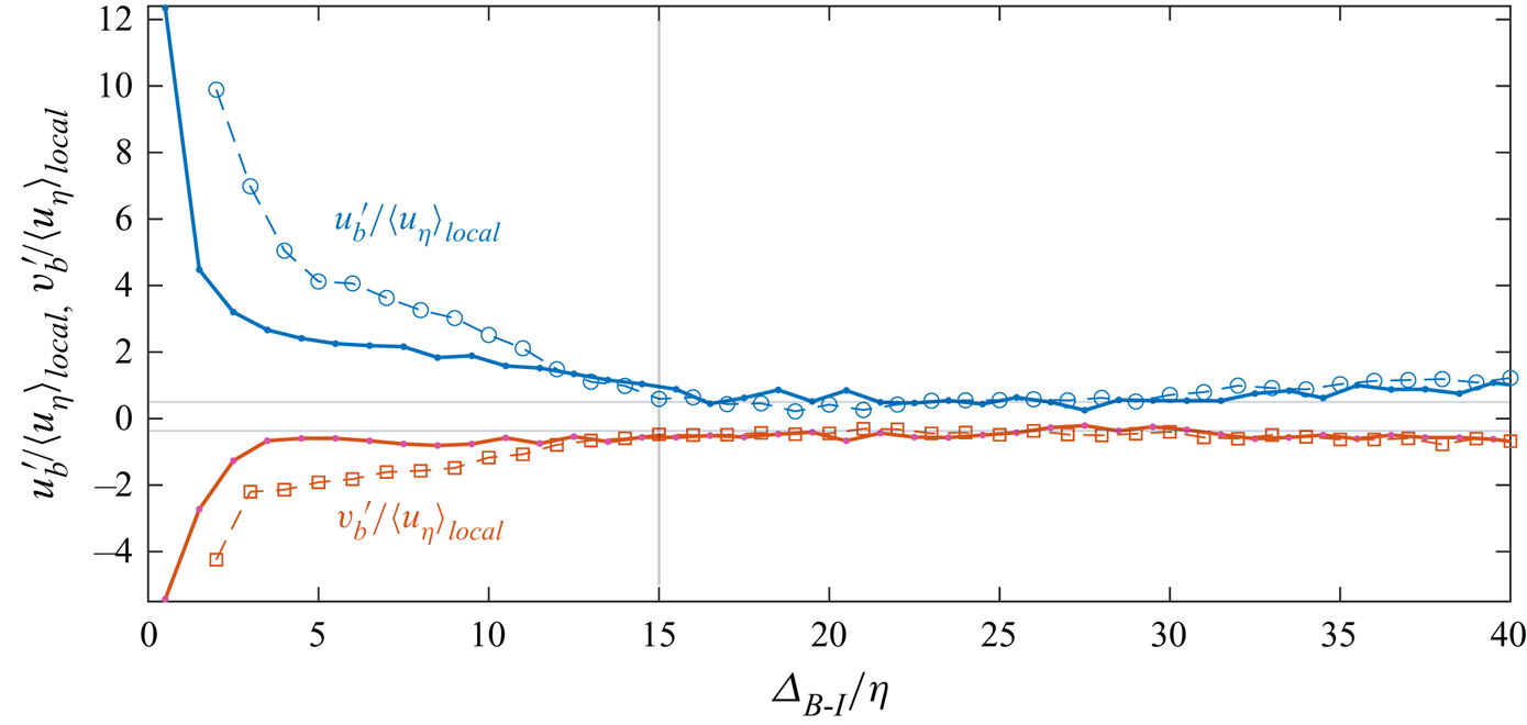
In figure 7, the velocity fluctuation inside bubbles (denoted by the subscript  $b$) are conditional averaged based on the distance from the TNTI to the centroid of the bubble. Bubbles inside the TNTI (
 $\varDelta_{B-I}<15\eta$) can be found to contain greater positive
 $u'$ and negative
 $v'$; in the meanwhile, the velocity fluctuations do not scale with the local Kolmogorov velocity scale. These evidences suggest that these bubbles are more likely to be engulfed into the turbulent region by the intense large-scale sweep events near the TNTI. In contrast, for the bubbles far away from the TNTI (
 $\varDelta_{B-I}>15\eta$), the velocity fluctuations are quite small, and can be scaled with the local Kolmogorov velocity scale. These phenomena imply that these bubbles are more likely to be produced by the local small-scale turbulent activities, and are not strongly related to engulfment. Thus, it is reasonable to separate the two kinds of bubbles by their distances from the TNTI. Noted that the results from the DNS data qualitatively are consistent with the experimental results, which verifies the reliability of our observations.
Velocity fluctuations inside bubbles as functions of  $\varDelta_{B-I}$. The velocity fluctuations are normalized by the local Kolmogorov velocity scale
 $\langle u_\eta \rangle _{local}$. Dash curves, results from the experimental data; solid curves, results from the DNS data.

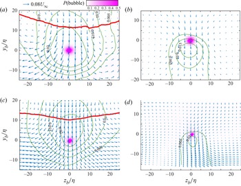
The velocity fields around the bubbles with  $\varDelta_{B-I}< 15\eta$ and
 $\varDelta_{B-I}> 15\eta$ in the
 $z$–
 $y$ plane are further conditionally averaged in figure 8. The origin is set at the centroid of the bubbles. For bubbles inside the TNTI (figure 8a,c), the bubbles are roughly at the centre of a large-scale Q4 event, and the TNTI above sinks. These all verify that the bubbles originate from the non-turbulent region, and are engulfed though sweep events. For bubbles with
 $\varDelta_{B-I}> 15\eta$ (figure 8b,d), the conditional-averaged velocity fields are quite different. The bubbles are still related to the sweep events, but the spanwise scale of the sweep event is smaller (
 $O(10\eta )$). In the meanwhile, the location of the bubble is at the top of the sweep event where the velocity fluctuation is not the strongest. These differences again suggest that the formation mechanisms are different for bubbles inside and outside the TNTI. More intuitive visualizations can be found in the
 $x$–
 $y$ plane with the same conditional average method. However, due to the absence of 3-D data in experiments, only the results from the DNS data are presented in figure 9 as a reference. In figure 9(a), the bubble is below the wedge-shaped deformation of the TNTI, and is inside a large-scale sweep event, which are consistent with the observations in figure 8(a,c). Figure 9(b) further shows that bubbles far away from the TNTI tend to be located at the downstream of sweep events where
 $-\partial u /\partial x$ is large. According to the research by Wang, Pan & Wang (Reference Wang, Pan and Wang2021), the regions with intense
 $-\partial u /\partial x$ are related to the inverse energy cascade (the phenomenon that turbulent kinetic energy is transported from small-scale motions towards large-scale motions). The loss of energy in small-scale motions could induce the formation of local small-scale non-turbulent regions, i.e. bubbles. Further investigations are still required to verify this conjecture.
Conditional averaged flow fields in the vicinity of bubbles in the  $z$–
 $y$ plane: (a) experimental data,
 $\varDelta_{B-I}<15\eta$; (b) experimental data,
 $\varDelta_{B-I}>15\eta$; (c) DNS data,
 $\varDelta_{B-I}<15\eta$; (d) DNS data,
 $\varDelta_{B-I}>15\eta$. Blue arrows, the vertical and spanwise velocity fluctuations
 $v'/U_{\infty }$ and
 $w'/U_{\infty }$, one of every three vectors is displayed for brevity; green contour lines, the streamwise velocity fluctuations
 $u'/U_{\infty }$; red curves, the conditional-averaged location of TNTI; purple-coloured background, the occurrence probability of bubbles.

Conditional averaged flow fields in the vicinity of bubbles in the  $x$–
 $y$ plane: (a) DNS data,
 $\varDelta_{B-I}<15\eta$; (b) DNS data,
 $\varDelta_{B-I}>15\eta$. Blue arrows, the streamwise and spanwise velocity fluctuations
 $u'/U_{\infty }$ and
 $w'/U_{\infty }$, one of every three vectors is displayed for brevity; red curves, the conditional-averaged location of TNTI; purple-coloured background, the occurrence probability of bubbles.

Based on these observations,  $\varDelta _{thre}$ is selected to be
 $15\eta$. To obtain the engulfment flux, the time interval
 $\Delta t_b$ also needs to be determined. Here
 $\Delta t_b$ is estimated as the averaged time for engulfed bubbles to reach their current position. First, the relative velocity of bubbles towards the TNTI is estimated by subtracting the velocity of the TNTI nearest to the bubble from the averaged velocity inside the bubble. The acquired average relative velocity is
 $O(v_{\eta })$ for bubbles inside the TNTI in both experimental and DNS data. Second, the mean distance from the TNTI to the centroid of an engulfed bubble is obtained by averaging
 $\varDelta_{B-I}$ for bubbles with
 $\varDelta_{B-I}<\varDelta _{thre}$. Hence,
 $\Delta t_b$ is determined as
 \begin{equation} \Delta t_b = \langle \varDelta_{B-I} \rangle_{\varDelta_{B-I}<\varDelta_{thre}}/v_{\eta}. \end{equation}
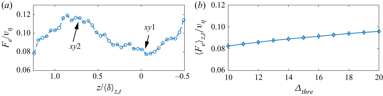
The obtained  $F_e$ is presented in figure 10(a). Here,
 $F_e$ is much larger in the H-SM regions than in the L-SM region. According to the above analysis, this is due to the sweep events in the H-SM regions which brings more irrotational bubbles directly into the turbulent region. The robustness of the flux estimation is checked in figure 10(b). Varying
 $\varDelta _{thre}$ by
 $\pm 5\eta$, the variation of
 $\langle F_e \rangle _{z,t}$ is approximately
 ${\pm }8\,\%$. The slight increment of engulfment flux against
 $\varDelta _{thre}$ could be attributed to including bubbles which do not originate from engulfment. Nevertheless, the variation is not large, indicating that the present estimation of
 $F_e$ is reasonable. Based on the above observations, it is concluded that the engulfment is enhanced in the vicinity of H-SMs due to the stronger sweep flow.
(a) Spanwise distribution of engulfment flux per wall unit  $F_e$. (b) Ratio of
 $F_e$ over H-SM against
 $F_e$ over L-SM.

3.3. Entrainment properties: nibbling flux
As for the nibbling rate, it has been shown that the tortuosity is larger above the H-SM in § 3.1. So here, the entrainment velocity  $v_n$ will be the focus.
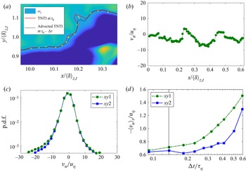
Here,  $v_n$ is obtained with the method proposed by Wolf et al. (Reference Wolf, Lüthi, Holzner, Krug, Kinzelbach and Tsinober2012), in which the movements of the TNTI relative to the fluid are considered as the result of nibbling. Figure 11(a) illustrates the calculation process. First, the TNTI at one instant
 $t_0$ is detected, as shown by the red curve. Second, the TNTI at a short time interval before (
 $t_0-\Delta t$) is advected with the local velocity to the current instant, as shown by the black dash curve. Third, the entrainment velocity is obtained by dividing the normal distance from the current TNTI to the advected TNTI with the advection time
 $\Delta t$. In the present work,
 $v_n <0$ represents the non-turbulent fluids becoming turbulent, and
 $v_n >0$ the turbulent fluids becoming non-turbulent. An example of the acquired instantaneous entrainment velocity is presented in figure 11(b). It is worth noting that the original method proposed by Wolf et al. (Reference Wolf, Lüthi, Holzner, Krug, Kinzelbach and Tsinober2012) is applied to a three-dimensional velocity field, but here it is used in two-dimensional PIV data. So strictly speaking, the acquired
 $v_n$ is the projection of the entrainment velocity on the
 $x$–
 $y$ plane. However, as shown by Mistry et al. (Reference Mistry, Philip, Dawson and Marusic2016) and Kankanwadi & Buxton (Reference Kankanwadi and Buxton2020),
 $v_n$ acquired from the
 $x$–
 $y$ plane is able to reflect the dominant entrainment events. Moreover, the p.d.f.s of
 $v_n$ (figure 11c) are qualitatively in good agreement with the results in Wolf et al. (Reference Wolf, Lüthi, Holzner, Krug, Kinzelbach and Tsinober2012): both p.d.f.s are non-Gaussian, with the wide tails on both sides; and both p.d.f.s have negative skewness, which shows the outwards spreading tendency of the turbulent region. The robustness of the acquired
 $v_n$ is further checked in figure 11(d). By varying the tracking interval
 $\Delta t$, it is found that the time-mean entrainment velocity is almost invariant for short tracking interval (
 $\Delta t <0.3 \tau _{\eta }$, where
 $\tau _{\eta }$ is the Kolmogorov time scale averaged at the TNTI location). In the present work,
 $\Delta t$ is selected as
 $0.14 \tau _{\eta }$, as marked by the grey line in figure 11(d). The obtained mean
 $v_n$ at the planes
 $xy1$ and
 $xy2$ are
 $-0.71v_{\eta }$ and
 $-0.66 v_{\eta }$, respectively, which are close to the values reported by Wolf et al. (Reference Wolf, Lüthi, Holzner, Krug, Kinzelbach and Tsinober2012) (
 $\approx 0.7 v_{\eta }$) and Mistry et al. (Reference Mistry, Philip and Dawson2019) (
 $0.68 v_{\eta }$). Here,
 $v_{\eta }$ is the Kolmogorov velocity scale averaged at the location of the TNTI (Marco & da Silva Reference Marco and da Silva2021).
(a) Illustration of the entrainment velocity calculation process; the red curve is the TNTI at  $t_0$; the dashed black curve is the TNTI at
 $t_0-\Delta t$ (advected with the local velocity). (b) A sample instantaneous entrainment velocity profile measured in the plane
 $xy1$. (c) Probability distributions of entrainment velocity in the two planes. (d) Variation of the time-mean entrainment velocity
 $\langle v_n \rangle _t$ against the advection time
 $\Delta t$.

Another way to obtain  $v_n$ is through the formula of entrainment velocity (Holzner & Lüthi Reference Holzner and Lüthi2011). Theoretically,
 $v_n$ is formed as
 \begin{align} v_n&={-}\frac{2\omega_i \omega_j s_{ij}}{|\boldsymbol{\nabla} \omega^2 |}-\frac{\nu \boldsymbol{\nabla} \boldsymbol{\cdot} (\boldsymbol{\nabla} \omega^2)}{|\boldsymbol{\nabla} \omega^2 |}+\frac{2\nu \boldsymbol{\nabla} \omega_i\boldsymbol{\cdot} \boldsymbol{\nabla} \omega_i}{|\boldsymbol{\nabla} \omega^2 |}\nonumber\\ &={-}\frac{P_{\omega}}{|\boldsymbol{\nabla} \omega^2 |}-\frac{D_{\omega}}{|\boldsymbol{\nabla} \omega^2 |}-\frac{\epsilon_{\omega}}{|\boldsymbol{\nabla} \omega^2 |} = v_{P}+v_{D}+v_{\epsilon}. \end{align}
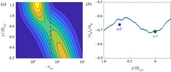
However,  $-\epsilon _{\omega }$ is a squared term which is always positive. This property implies the noise disturbance can not be eliminated by simply taking the temporal average (an example is that in figure 2(c),
 $\langle \epsilon _{\omega } \rangle$ is not zero in the non-turbulent region). Hence, direct calculation through (3.5) will lead to biased results. To minimize the disturbance of noise,
 $-\epsilon _{\omega }$ smaller than a selected threshold
 $\epsilon _{thre}$ is set to be 0 during the calculation. To determine
 $\epsilon _{thre}$, figure 12(a) shows the distribution of
 $-\epsilon _{\omega }$. Two regions can be identified: the large
 $-\epsilon _{\omega }$ region near the wall and the small
 $-\epsilon _{\omega }$ region far from the wall. Considering that the
 $-\epsilon _{\omega }$ should be negligible in the free stream, the
 $\epsilon _{thre}$ is chosen between the two regions, as shown by the dash line in figure 12(a). The obtained
 $\langle v_n \rangle _t$ is presented in figure 12(b). The results from the two methods are consistent with each other, indicating the effectiveness.


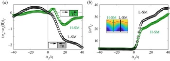
It can be found that the entrainment velocity tends to be larger above the L-SM, which illustrates L-SM could induce stronger instantaneous entrainment events. It is proposed that the L-SMs enhance  $v_n$ through the instantaneous flow direction related to the TNTI. When an instantaneous flow moves towards the TNTI, it has been observed that the nearby vortices tend to be stretched due to the alignment between the vorticity vector and the first eigenvector of the strain-rate tensor (Watanabe et al. Reference Watanabe, Sakai, Nagata, Ito and Hayase2014; Mistry et al. Reference Mistry, Philip and Dawson2019). Vortex stretching will enhance the enstrophy production, thus increasing
 $v_n$ (Holzner et al. Reference Holzner, Lüthi, Tsinober and Kinzelbach2009; Holzner & Lüthi Reference Holzner and Lüthi2011). In a time-mean sense, L-SMs are statistically accompanied by upwards flow, bringing the fluid towards the TNTI, while H-SMs are the opposite. To show the flow direction in detail, the conditional-averaged flow direction related to the TNTI in the planes
 $xy1$ and
 $xy2$ is plotted in figure 13(a). Here,
 $u_n$ is the velocity along the local coordinate perpendicular to the TNTI and
 $u_n(0)$ is the
 $u_n$ at the TNTI location. Additionally,
 $u_n-u_n(0)>0$ means the flow moves towards the turbulent region. In a turbulent region,
 $u_n-u_n(0)$ decreases faster in the plane
 $xy1$, suggesting that more fluids are transported towards the TNTI. This enhances the enstrophy production near the TNTI. Moreover, with more enstrophy brought towards the TNTI and more enstrophy production, it can be deduced that the vorticity jump across the TNTI will be larger above the L-SM, which is verified in figure 13(b). This could also enhance the viscous diffusion
 $v_{D}$, thus inducing stronger
 $v_n$ above the L-SM (Watanabe et al. Reference Watanabe, Sakai, Nagata, Ito and Hayase2014; Mistry et al. Reference Mistry, Philip and Dawson2019). In contrast, the flow moves away from the TNTI in the H-SM region, resulting in the smaller
 $v_n$. From another point of view, an intuitive explanation can be drawn from the modulation effect of velocity fluctuations introduced by Marusic, Mathis & Hutchins (Reference Marusic, Mathis and Hutchins2010): in the outer region of a TBL, small-scale fluctuations tend to be more energetic in the L-SM regions, which induces stronger nibbling events.
(a) Fluid velocity related to the TNTI. Here,  $\Delta _I$ is the distance to the TNTI and
 $\Delta _I >0$ is the turbulent region (also denoted as TR in the figure). (b) Conditional-averaged enstrophy profile along the local coordinate perpendicular to the TNTI.

However, the larger instantaneous  $v_n$ does not suggest that the local nibbling flux is larger, because
 $F_n$ is influenced by both entrainment velocity and the TNTI tortuosity. Actually, the obtained
 $F_n$ over L-SM and H-SM are 1.63
 $v_{\eta }$ and 1.71
 $v_{\eta }$, respectively (1.60
 $v_{\eta }$ and 1.66
 $v_{\eta }$ through (3.5)). It means that although extreme nibbling events are more likely to appear over L-SM, the total flux are still larger over H-SM due to the more distorted TNTI. As shown in figure 11(c), the distinct difference of the mean
 $v_n$ is mainly attributed to the large values whose occurrence probability is quite small. This is consistent with previous works (Holzner & Lüthi Reference Holzner and Lüthi2011; Mistry et al. Reference Mistry, Philip, Dawson and Marusic2016). For the nibbling rate, which is the integral of
 $v_n$ along TNTI, the nibbling flux is still slightly stronger above H-SMs due to the increased surface area in our experiments.
Additionally, it can be found that the nibbling flux is much greater than the engulfment flux. Over both H-SM and L-SM, the engulfment flux is approximately 5.5 % of the total entrainment flux. It should be noted that in the experiments, small-scale bubbles are ignored to avoid noise disturbance. Thus, the present work could underestimate the engulfment flux. If we assume that the p.d.f. of the bubble radius follows the  $-3$ power law and the smallest radius of the bubble is
 $1\eta$ (da Silva et al. Reference da Silva, Taveira and Borrell2014b), the total area of ignored bubbles can be estimated; then the engulfment flux could be approximately 7 % of the total entrainment flux, which is consistent with the ratio (4–8 %) reported by Jahanbakhshi & Madnia (Reference Jahanbakhshi and Madnia2016).
4. Universal modulations on entrainment
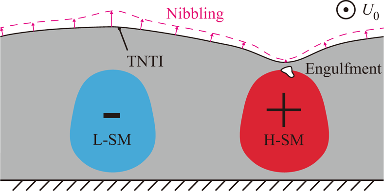
Based on the above observations, a conceptual model of H/L-SMs on the entrainment process could be extracted, as illustrated in figure 14. The L-SMs will enlarge the instantaneous entrainment velocity  $v_n$, while the H-SMs will increase the volume of engulfed irrotational fluids and TNTI tortuosity. As a result, it is above the H-SMs that both the nibbling flux and engulfment flux are stronger.
Conceptual model for the modulations of large-scale motions on the turbulent entrainment. The entrainment velocity is illustrated by pink arrows.

To show the model could be universal for TBLs, the effectiveness of the model is checked with different wall conditions. For this purpose, two sets of data are investigated here: one set of the TBL over a smooth wall ( $Re_{\tau } \approx 1500$) simulated by direct numerical simulation and one set of the TBL over homogeneous roughness (
 $Re_{\tau } \approx 700$) acquired by experiments. The occurrence locations of H/L-SMs are random in these TBLs, which means that the conclusions drawn from these data could be universal for various wall shapes.
The instantaneous H/L-SMs are detected through the method proposed by Lee et al. (Reference Lee, Sung and Zaki2017), in which the peaks and valleys of filtered  $u'$ in the
 $y$–
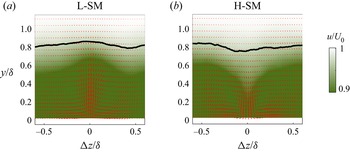
 $z$ plane are considered as the ‘cores’ of H/L-SMs. The statistical shapes of H/L-SMs are presented in figure 15(a,b), in which the velocity fields are conditional averaged around ‘cores’ of H/L-SMs for the smooth-wall TBL data. It can be seen that H/L-SMs are accompanied by downward/upward flow; and statistically, the TNTI elevates above the L-SM and sinks above the H-SM. These observations are consistent with those of Lee et al. (Reference Lee, Sung and Zaki2017), showing that the detection of H/L-SMs here is reliable. The results from homogeneous roughness data are also consistent with figure 15(a,b), and are presented in figure 18(a,d). The influence of different velocity fluctuation calculation methods is checked in Appendix A.
Conditional-averaged cross-section velocity distributions of (a) H-SM and (b) L-SM; red arrows, in-plane velocity. The results are obtained from DNS data of the TBL over a smooth wall.

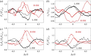
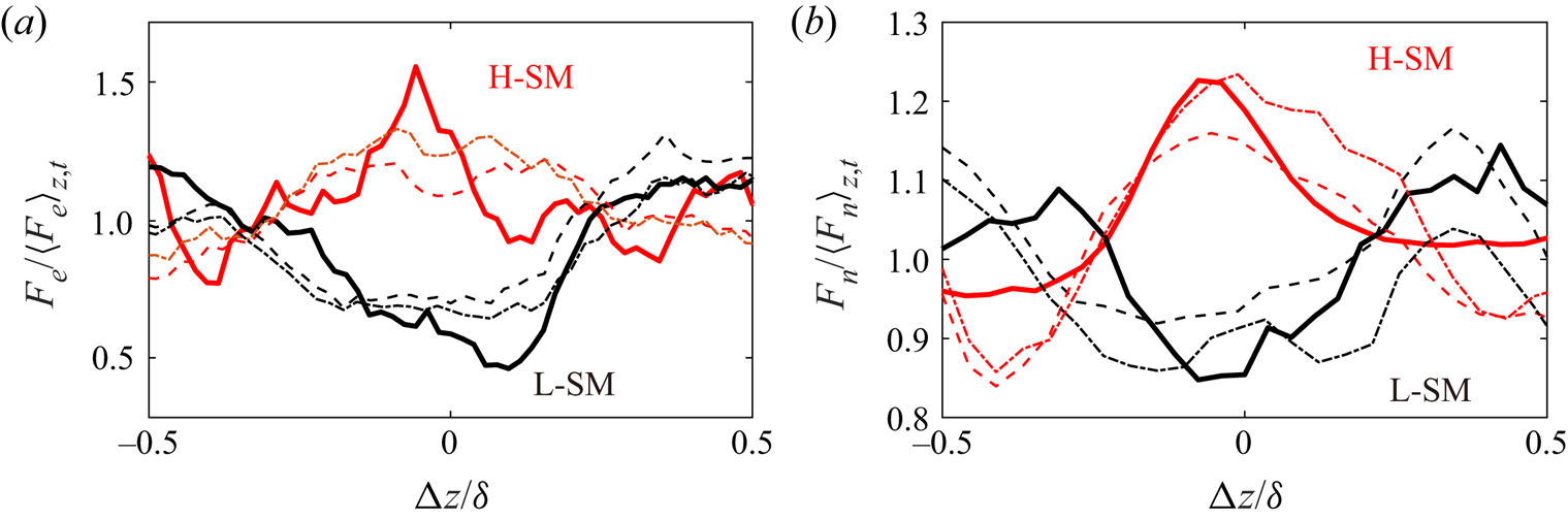
The engulfment flux  $F_e$ in the vicinity of H/L-SMs are shown in figure 16(a). Similar with the results in spanwise heterogeneity, bubbles tend to appear in the H-SM region (red curves in figure 16a) and vanish in the H-SM region (black curves in figure 16a). It can be seen that the influenced range of H/L-SMs on
 $F_e$ is approximately
 $\pm 0.2 \delta _{99}$. This range is reminiscent of the two-point correlation function of
 $v$ whose spanwise scale is also approximately
 $0.4 \delta _{99}$ (Sillero et al. Reference Sillero, Jiménez and Moser2014; Jiménez Reference Jiménez2018). This consistency again confirms that the formation of bubbles is mainly modulated by downward flow. It is interesting to notice that on both spanwise sides of L-SM, there are areas with weak downward flows. Correspondingly,
 $F_e$ at
 $\pm 0.4 \delta _{99}$ is slightly larger than the mean value. Similar observations can also be seen around H-SM.
Distribution of (a) engulfment flux  $F_{e}$, (b) entrainment velocity
 $v_n$, (c) tortuosity of TNTI
 $L_I/L_x$ and (d) nibbling flux
 $F_n$ in the vicinity of H/L-SMs. Here,
 $\Delta z = 0$ is the location of the ‘core’ of H-SM (red curves) and L-SM (black curves). Solid curves, TBL over smooth wall (DNS data); dash curves, TBL over homogeneous roughness (experimental data).

The variations of  $v_n$ are further plotted in figure 16(b). Here
 $v_n$ is obtained by (3.5). During calculating with the experimental data, the modification method described in figure 12(a) is also applied to avoid noise disturbance. Consistent with the last section, the mean value of
 $v_n$ is increased above L-SMs and decreased above H-SMs. Compared with the distributions of
 $F_e$, the range in which the H/L-SMs influence
 $v_n$ is wider (
 $\approx \pm 0.4 \delta _{99}$). This value is close to the spanwise auto-correlation scale of
 $u'$ (Sillero et al. Reference Sillero, Jiménez and Moser2014; Jiménez Reference Jiménez2018), which means that the flow direction related to the TNTI is mainly affected by the streamwise velocity. This is also illustrated by Watanabe et al. (Reference Watanabe, Sakai, Nagata, Ito and Hayase2014). The deviations of
 $v_n$ from the mean value are approximately 5–10 % for both H/L-SMs, which are larger than the deviations over heterogeneous and homogeneous. The reason is that the H/L-SMs over heterogeneity will meander in the instantaneous flow, which will smooth the difference.
However, as have been shown in § 3.3, the large  $v_n$ does not indicate a large local nibbling flux, because the influence from the TNTI tortuosity cannot be ignored. In figure 16(c), the tortuosities near the H/L-SMs are illustrated. In the vicinity of H-SM, the tortuosity is approximately 30 % higher than the average value in both the experimental and DNS data. This deviation is significantly larger than that of
 $v_n$. Consequently, the nibbling rate is larger above H-SM (figure 16d) due to the violently distorted TNTI.
In conclusion, the total entrainment flux is larger over the H-SM and smaller over the L-SM. Compared to the time-averaged values, the increment over H-SM is approximately 50 % for the engulfment flux and 15–20 % for the nibbling flux in the present experimental and numerical data. The ratios of the engulfment flux in the total entrainment flux is approximately 5 % in both datasets. Hence, the total flux depends predominately on the nibbling flux.
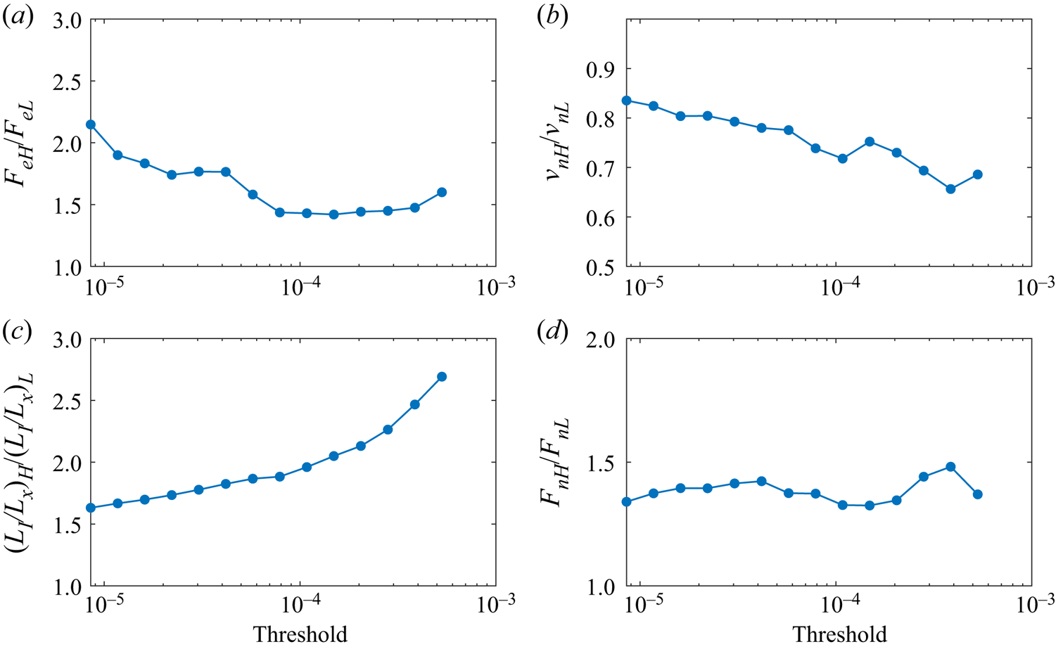
Moreover, since the enstrophy-related quantities in the vicinity of the TNTI change rapidly, it is essential to check the effectiveness of our conclusions with different TNTI detection thresholds. In figure 17, we present the ratios of the entrainment rate of H-SM to L-SM over three orders of threshold values ( $\omega ^2=0(10^{-5}) \sim O(10^{-3})$). It can be visible that the conclusions are invariant for all the threshold values. The ratio of the engulfment flux in figure 17(a) decreases slightly with increasing threshold. The reason is that some bubbles are directly connected with the TNTI. Moreover, it is interesting to notice that although the ratio of
 $v_n$ declines (figure 17b), the ratio of nibbling flux is balanced by the growing ratio of the TNTI tortuosity (figure 17c). As a result, the ratio of the nibbling flux stays at approximately 1.4 for all the thresholds used here (figure 17d).
Ratios of (a) engulfment flux  $F_e$, (b) entrainment velocity
 $v_n$, (c) tortuosity of TNTI
 $L_I/L_x$ and (d) nibbling flux
 $F_n$ over H-SM and L-SM under different TNTI detection thresholds. The results are obtained from the DNS data. The threshold used in figure 16 is
 $1\times 10^{-5}$.

5. Conclusions
In this paper, the universal modulations of  $\delta$-scaled large-scale motions on the TNTI and entrainment are explored. Turbulent boundary layers over three kinds of wall shapes (spanwise heterogeneous roughness, homogeneous roughness and smooth wall) are used to ensure the conclusions are universal for TBLs. Following previous works, the entrainment process is divided into two parts: engulfment (drawing pockets of irrotational flows directly into the turbulent region) and nibbling (vorticity propagation along the TNTI); and the instantaneous TNTI is detected as the isoline of enstrophy.
In the engulfment process, it is shown that bubbles close to the TNTI contain large positive  $u'$, and are more likely to originate from engulfment, while the bubbles far from the TNTI contain large
 $-\partial u'/\partial x$, and could be produced by the local turbulence itself. Moreover, the H-SM will increase the local engulfment flux up to 150 % of the mean value. The reason is attributed to the sweep flow in the H-SM region.
In the nibbling process, it is found that the tortuosity of the TNTI and the entrainment velocity play opposite roles over H/L-SMs. The tortuosity is larger over H-SM due to the influence from both small-scale and large-scale motions. The entrainment velocity is larger over L-SM due to the upwards flow towards the TNTI. In summary, the nibbling flux is larger over H-SM up to 120 % of the mean value, because the variation of tortuosity is significantly larger than the entrainment velocity.
The conclusions above are further verified for different wall shapes and various TNTI detection thresholds, which shows that the conclusions could be universal for turbulent boundary layers.
Acknowledgements
The authors sincerely thank Professor J. Jiménez for providing the DNS data set for analysis.
Funding
This work was supported by National Natural Science Foundation of China (grant numbers 91852206, 11721202).
Declaration of interests
The authors report no conflict of interest.
Data availability statement
The DNS data of turbulent boundary layer over smooth wall at  $Re_{\tau }=1500$ can be obtained from the open High-Reynolds-Numbers DNS Turbulent Boundary Layer Data from University Politecnica de Madrid (https://torroja.dmt.upm.es/turbdata/blayers/). The experimental data that support the findings of this study are available from the corresponding author upon reasonable request.
Appendix A. The influence of different fluctuation velocity calculation methods
In this work, the fluctuation velocity  $u^{\prime }$ is calculated by subtracting the time-averaged velocity
 $\langle u \rangle_t$ from the instantaneous velocity u, i.e.
 \begin{equation} u^{\prime} = u-\langle u \rangle _{t}. \end{equation}
Equation (A1) is also known as the conventional Reynolds decomposition. In consideration of the intermittency of turbulence, two other decomposition methods have also been proposed. The first method is used by Lee et al. (Reference Lee, Sung and Zaki2017). At a fixed point, the fluctuation velocity is calculated as
 \begin{equation} u'=\left\{ \begin{array}{ll} u-\langle u \rangle _T, & {\rm if}\ {\omega^2 \ge\omega^2_{th}}\ (\text{turbulent}),\\ u-\langle u \rangle _{NT}, & {\rm if}\ {\omega^2 <\omega^2_{th}}\ (\text{non-turbulent}),\\ \end{array} \right. \end{equation}
where  $\langle \rangle _T$ and
 $\langle \rangle _{NT}$ are taking the average when the flow is turbulent and non-turbulent, respectively. The second method is proposed by Kwon, Hutchins & Monty (Reference Kwon, Hutchins and Monty2016). In this new decomposition, the subtracted mean velocity profile depends on the instantaneous TNTI height
 $y_I$, i.e.
 \begin{equation} u'=u-\langle u \rangle_{t|y_I}. \end{equation}
Both methods are designed to remove the velocity fluctuations in the non-turbulent free stream.
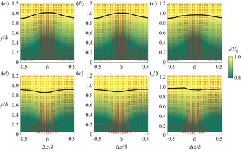
The ‘cores’ of large-scale motions are detected in the  $u'$ fields obtained from the three methods, and the conditional-averaged velocity fields are presented in figure 18. The obtained fields are quite similar except for the flatter TNTIs in figure 18(c,f). The reason is that the velocity component highly correlated with the TNTI height has been subtracted in (A3). Hence, the
 $u'$ is less correlated with the TNTI height, and the TNTI are flatter in the conditional-averaged fields. Nevertheless, the phenomena are qualitatively similar: the TNTI sinks over the H-SM and elevates over the L-SM. The fluxes of engulfment and nibbling are further plotted in figure 19. In all the three cases,
 $F_e$ and
 $F_n$ are higher over the H-SM, which indicates that the conclusions in the present work do not depend on the method of obtaining
 $v_n$.
Conditional-averaged cross-section velocity distributions of L-SM (a–c) and H-SM (d–f); the ‘cores’ of large-scale motions are detected in the  $u'$ field obtained from (a,d) (A1), (b,e) (A2) and (c,f) (A3). The black curves are the time-mean TNTI location. The results are from the experimental data over homogeneous roughness.


Appendix B. The effectiveness of bubble detection
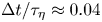
A key concern on the bubble detection is how to separate bubbles from the irrotational regions directly connected to the free stream (referred as ‘pockets’ hereinafter). In our bubble detection procedure, the pockets are removed by the following steps.
(i) First, since the SPIV data in our work are time-resolved (
 $\Delta t/\tau _{\eta }\approx 0.04$), the bubbles which are at the same location in two adjacent frames are considered as the same bubble.
(ii) Second, bubbles which are directly connected with the non-turbulent region in any frame are removed from all the frames.
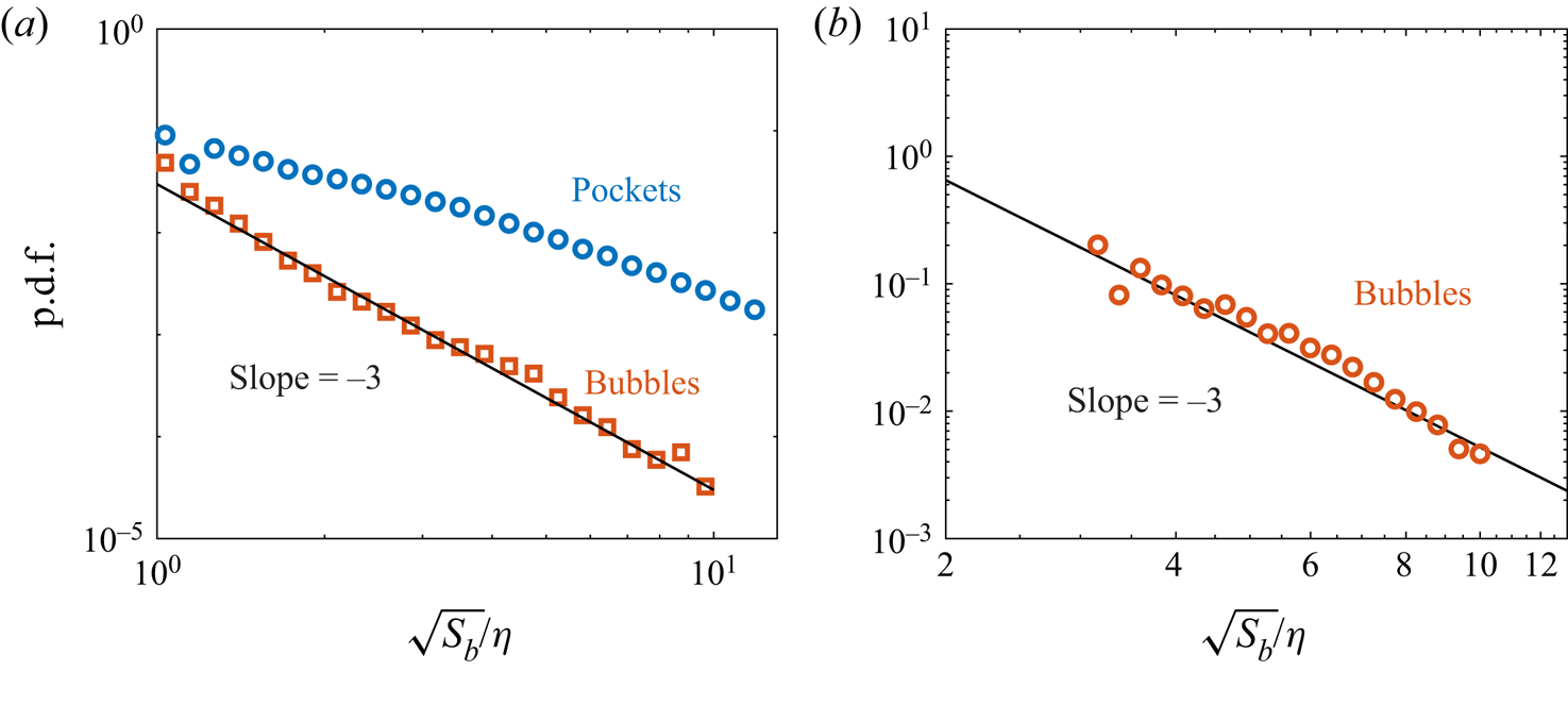
To verify the effectiveness of our bubble detection procedure, the 2-D DNS slices in the spanwise-vertical plane are analyzed. Bubbles and the ‘pockets’ are recognized separately in the 2-D DNS slices. The probability distribution function (p.d.f.) of the radius of bubbles and ‘pockets’ are plotted in figure 20(a). It can be found that the p.d.f. of bubbles follows a  $-$3 power law. This is also report by da Silva et al. (Reference da Silva, Taveira and Borrell2014b) and Jahanbakhshi & Madnia (Reference Jahanbakhshi and Madnia2016). As a contrast, the p.d.f. of ‘pockets’ does not follow the
 $-$3 power law. Figure 20(b) further shows the p.d.f. of the bubble radius in our experiments, which also fits the
 $-$3 slope. The result shows that the ‘pockets’ have been effectively excluded in our bubble detection procedure.
Probability distribution function of bubble radius in the (a) 2-D DNS slice and (b) experimental data.