


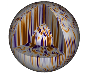


1 Introduction
Convection plays a key role in the interior dynamics of many planets and stars. Spherical geometry and rotation are important in many of these natural convecting systems, including Earth’s liquid metal outer core, solar and stellar interiors, and planetary atmospheres. The length scales associated with core convection in the Earth, range from narrow columns of the order of 10 m to system size flow structures (Jones Reference Jones and Schubert2015). Similarly the range of time scales varies from the rotation period on the diurnal scale, to magneto-Coriolis waves on the decadal scale, and geomagnetic reversals which occur on average a few times every million years (Holme Reference Holme2007). The convective state of these astrophysical and geophysical systems, and the resulting heat transport, cannot be probed directly via numerical or physical experiment as the parameters of the system give rise to highly complex spatial and temporal behaviour. Consequently, a large body of work exists (described below) deriving and testing scaling relationships between the independent and dependent variables. This paper is motivated by convection in planetary cores where the effects of rotation and spherical geometry are important in determining the dynamics. We focus here on how rotation affects the scaling behaviour of both global and local diagnostics describing the heat transport (Nusselt number, interior temperature gradients, interior temperatures, thermal boundary layers) and flow properties (Reynolds number, convective length scales, viscous boundary layers). In what follows we will discuss the different scaling behaviours previously observed in both the plane-layer and spherical shell geometries and the different physical regimes of rotating convection, all of which is discussed for Boussinesq convection.
1.1 Rayleigh–Bénard convection in a plane layer
Rayleigh–Bénard convection (RBC) is a paradigm problem of convective fluid dynamics; the addition of rotation provides a simplified dynamical analogue for many planetary and stellar systems. The RBC paradigm consists of a fluid contained between two rigid horizontal plates with gravity acting perpendicular to the plates. A sufficiently high temperature difference  $\unicode[STIX]{x0394}T$ is maintained between the boundaries to destabilise the fluid layer. For a given aspect ratio the non-dimensional parameters governing the system are the Rayleigh number,
 $Ra$, and Prandtl number,
 $Pr$ (see table 1). The effect of rotation, when present, is encapsulated by a third non-dimensional parameter, the Ekman number,
 $E$, which measures the relative importance of viscosity to rotation.
Dimensionless parameters governing rotating convection. Here  $\unicode[STIX]{x1D708}$ is the fluid’s viscous diffusivity,
 $\unicode[STIX]{x1D6FA}$ is the angular rotation rate,
 $h$ is the depth of the fluid layer,
 $\unicode[STIX]{x1D705}$ is the thermal diffusivity,
 $\unicode[STIX]{x1D6FC}$ is the coefficient of thermal expansion,
 $g_{o}$ is the gravitational acceleration,
 $\unicode[STIX]{x1D6FD}$ is a measure of the imposed heat flux and
 $\unicode[STIX]{x0394}T$ is the temperature drop across the fluid layer. The modified Rayleigh number
 $\widetilde{Ra}$ is the rotational flux Rayleigh number and is used as an input parameter in this study. Note that
 $\widetilde{Ra}$ can be transformed to the traditional Rayleigh number,
 $Ra$ as follows:
 $Ra\propto \widetilde{Ra}/(ENu)$ where the constant of proportionality is a geometric factor. A radius ratio
 $r_{i}/r_{o}=0.35$ is used throughout.

Rotating RBC has been shown to display dynamics in one of two regimes; rapidly rotating (RR) and weakly rotating (WR) as evidenced by global heat transfer behaviour measured by the Nusselt number,  $Nu$ (e.g. King et al. Reference King, Stellmach, Noir, Hansen and Aurnou2009; Schmitz & Tilgner Reference Schmitz and Tilgner2010), defined as the ratio of the total heat transport (sum of convective and conductive contributions) to the conductive heat transport. Here, we briefly review some relevant results for rotating RBC and refer the reader to Plumley & Julien (Reference Plumley and Julien2019) for a detailed discussion of
 $Nu$–
 $Ra$ behaviour. RR convection exhibits suppressed heat transfer relative to non-rotating convection with the scaling exponent increasing monotonically with decreasing Ekman number,
 $Nu\sim Ra^{\unicode[STIX]{x1D706}(E)}$ (e.g. Cheng et al. Reference Cheng, Stellmach, Ribeiro, Grannan, King and Aurnou2015; Kunnen et al. Reference Kunnen, Ostilla-Mónico, van der Poel, Verzicco and Lohse2016). Plane layer simulations with stress-free boundaries find that the heat transport saturates at the asymptotic scaling
 $Nu\sim Ra^{3/2}E^{2}$ (Julien et al. Reference Julien, Knobloch, Rubio and Vasil2012a). In the no-slip case, however, the presence of Ekman boundary layer effects can enhance the heat transport leading to larger scaling exponents (e.g. Stellmach et al. Reference Stellmach, Lischper, Julien, Vasil, Cheng, Ribeiro, King and Aurnou2014; Plumley et al. Reference Plumley, Julien, Marti and Stellmach2016) such as those observed by Cheng et al. (Reference Cheng, Stellmach, Ribeiro, Grannan, King and Aurnou2015) and Kunnen et al. (Reference Kunnen, Ostilla-Mónico, van der Poel, Verzicco and Lohse2016). Heat transfer in the WR regime behaves similarly to that for convection without rotation: the empirical
 $Nu\sim Ra^{2/7}$ scaling is observed for moderate Rayleigh numbers (
 $Ra\leqslant 10^{10}$) before saturating at
 $Nu\sim Ra^{1/3}$ for sufficiently high values of
 $Ra$ (
 $Ra\geqslant 10^{10}$) (Cheng et al. Reference Cheng, Stellmach, Ribeiro, Grannan, King and Aurnou2015).
Three main parameters have been suggested to control the transition from RR to WR convection. King et al. (Reference King, Stellmach, Noir, Hansen and Aurnou2009) and King, Stellmach & Aurnou (Reference King, Stellmach and Aurnou2012) suggest that the transition between the RR and WR regimes occurs when the thermal boundary layer becomes thinner than the viscous boundary layer, occurring at either  $RaE^{7/4}\sim O(1)$ or
 $RaE^{3/2}\sim O(1)$ depending on whether
 $Nu\sim Ra^{2/7}$ or
 $Nu\sim Ra^{1/3}$ (for the range of
 $Ra$ studied here we find the
 $Nu\sim Ra^{2/7}$ scaling behaviour and consequently test the
 $RaE^{7/4}$ boundary layer crossing parameter, see § 2.3 for details). Alternatively, models with asymptotically small
 $E$ (Julien et al. Reference Julien, Rubio, Grooms and Knobloch2012b), suggest that the transition occurs when the thermal boundary layers are no longer in geostrophic balance, predicting a transition at
 $RaE^{8/5}\sim O(1)$. Other works advocate the convective Rossby number,
 $Ro_{c}=\sqrt{RaE^{2}/Pr}\sim O(1)$ (Gilman Reference Gilman1977) to demarcate the transition. There is no consensus on what controls the RR–WR transition and various other options have also been considered (see Cheng et al. (Reference Cheng, Aurnou, Julien and Kunnen2018) table 1 for an overview). The transition from RR to WR heat transfer behaviour is accompanied by vanishing interior temperature gradients,
 $\text{d}T_{int}$ (typically defined at mid-depth). Note that
 $\text{d}T_{int}$ scales inversely with supercriticality in the RR regime (Julien et al. Reference Julien, Rubio, Grooms and Knobloch2012b).
Despite the similar heat transfer behaviour between WR and non-rotating (NR) convection, the flow properties continue to be influenced by rotation even in the WR regime. The typical horizontal length scale associated with the convective flow follows the classic viscous scaling,  $\ell /h\sim E^{1/3}$ for both RR and WR convection (King, Stellmach & Buffett Reference King, Stellmach and Buffett2013). In contrast, for NR convection the flow exhibits three-dimensional turbulence and the typical length scale is then inversely proportional to the heat transport,
 $\ell /h\sim Nu^{-1/2}$ (King et al. Reference King, Stellmach and Buffett2013). Combining with the
 $Nu\sim Ra^{2/7}$ behaviour, one obtains
 $\ell /h\sim Ra^{-1/7}$. The Coriolis force does no work and it affects the convective flow speed (Reynolds number,
 $Re_{c}$) scaling solely by changing the length scales. A triple force balance between viscous, Archimedean and Coriolis forces (VAC balance) gives a scaling prediction for the flow speed,
 $Re_{c}\sim (Ra(Nu-1))^{1/2}E^{1/3}$ in both the RR and WR regimes (King et al. Reference King, Stellmach and Buffett2013). The different length scale observed in NR convection leads to a flow speed scaling,
 $Re_{c}\sim (Ra-Ra/Nu)^{1/2}$ (King et al. Reference King, Stellmach and Buffett2013).
A complete specification of the flow requires a description of the mechanical and thermal boundary layers. In the RR and WR regimes Coriolis forces balance viscosity in the region close to the walls leading to the Ekman boundary layer of thickness,  $\unicode[STIX]{x1D6FF}_{E}/h\sim E^{1/2}$ (Greenspan Reference Greenspan1968). In NR convection the Prandtl–Blasius theory (e.g. Kundu & Cohen Reference Kundu and Cohen1990) predicts a viscous boundary layer of thickness
 $\unicode[STIX]{x1D6FF}_{\unicode[STIX]{x1D708}}/h\sim Re_{c}^{-1/2}$. While some studies confirm this behaviour others find an empirical scaling,
 $\unicode[STIX]{x1D6FF}_{\unicode[STIX]{x1D708}}/h\sim Re_{c}^{-1/4}$ (Lam et al. Reference Lam, Shang, Zhou and Xia2002). This discrepancy was attributed to the boundary layers being either passive or active (Qiu & Xia Reference Qiu and Xia1998a,Reference Qiu and Xiab), however, more recent work has shown that the different scaling exponents follow from the adopted definition of the viscous boundary layer (Breuer et al. (Reference Breuer, Wessling, Schmalzl and Hansen2004), Gastine, Wicht & Aurnou (Reference Gastine, Wicht and Aurnou2015), see also figure 1(a) for the two different methods of defining a viscous boundary layer). Within the thermal boundary layers heat is transported almost purely by conduction and so for non-rotating convection the layer thickness scales as
 $\unicode[STIX]{x1D6FF}_{\unicode[STIX]{x1D705}}/h\sim Nu^{-1}$. This scaling is observed to hold in the WR regime and provides a reasonable first-order approximation in RR convection (King et al. Reference King, Stellmach and Buffett2013).
All of the results discussed above are from models with rotation and gravity aligned. There have been some investigations having the rotation axis tilted with respect to gravity and these systems are more complex in that they are capable of driving mean flows (Hathaway & Somerville Reference Hathaway and Somerville1983; Currie & Tobias Reference Currie and Tobias2016).
1.2 Spherical shell convection
In spherical shell convection the fluid is heated from the inner boundary and cooled at the outer boundary with gravity acting radially. Recently the first systematic study of rotating convection in a spherical shell geometry was published by Gastine, Wicht & Aubert (Reference Gastine, Wicht and Aubert2016). Similar to RBC, distinct regimes have been identified; and we follow Gastine et al. (Reference Gastine, Wicht and Aubert2016) by defining the weakly nonlinear (WN), rapidly rotating, transitional and non-rotating regimes. When comparing quantitatively with Gastine et al. (Reference Gastine, Wicht and Aurnou2015, Reference Gastine, Wicht and Aubert2016) we account for the factor two difference in their definition of the Ekman number.
Close to the onset of convection, the WN regime exists and persists for low values of supercriticality (e.g. Yadav et al. Reference Yadav, Gastine, Christensen, Duarte and Reiners2015). In this regime inertial forces are small and the heat transfer follows the perturbation analysis of Gillet & Jones (Reference Gillet and Jones2006),  $Nu-1\sim Ra/Ra_{c}-1$. Gastine et al. (Reference Gastine, Wicht and Aubert2016) found the WN regime exists for
 $Ra_{c}\leqslant Ra\leqslant 6Ra_{c}$, where
 $Ra_{c}$ is the critical value for instability. The RR regime is found for
 $E\leqslant 5\times 10^{-5}$ and is characterised by a steeper heat transfer scaling than the WN regime. As in the plane layer case the
 $Nu-Ra$ scaling exponents increase with decreasing
 $E$. Though Mound & Davies (Reference Mound and Davies2017) found a continuous increase for the parameter range considered, Gastine et al. (Reference Gastine, Wicht and Aubert2016) observed saturation at
 $Nu\propto Ra^{3/2}E^{2}$. This scaling might imply that an asymptotic regime has been reached as it is derived in the absence of thermal and viscous diffusion at asymptotically low
 $E$ (Jones Reference Jones and Schubert2015). The
 $Nu\propto Ra^{3/2}E^{2}$ heat transfer scaling is predicted to hold until the thermal boundary layer loses geostrophic balance, which defines a transition to WR convection when
 $RaE^{8/5}=O(1)$ (Julien et al. Reference Julien, Knobloch, Rubio and Vasil2012a). At numerically accessible values of
 $E$
 $({\geqslant}10^{-7})$ it is found that, above some transitional value of
 $Ra$, the
 $Nu-Ra$ scaling exponent continually changes in the transitional regime until the non-rotating scaling
 $Nu\sim Ra^{2/7}-Ra^{1/3}$ (Gastine et al. Reference Gastine, Wicht and Aurnou2015) is recovered in the NR regime. Gastine et al. (Reference Gastine, Wicht and Aubert2016) found that the heat transport scaling conforms to the NR behaviour when
 $Ra>328E^{-12/7}$. As in RBC the transition to the NR scaling occurs alongside vanishing interior temperature gradients (Gastine et al. Reference Gastine, Wicht and Aurnou2015).
The characteristic length scale and speed of the convective flow in the WN regime is described by the VAC balance, predicting  $\ell /h\sim E^{1/3}$ and
 $Re_{c}\sim (Ra(Nu-1))^{1/2}E^{1/3}$ (Gastine et al. Reference Gastine, Wicht and Aubert2016), as in rotating planar RBC. In the RR regime inertial effects dominate over viscous forces and Gastine et al. (Reference Gastine, Wicht and Aubert2016) found that the length scale approaches the Rhines scale of convection,
 $\ell /h\sim (Re_{c}E)^{1/2}$ (Rhines Reference Rhines1975) for
 $E=1.5\times 10^{-7}$. The appearance of the Rhines scale suggests that the fluid bulk has reached a triple force balance between inertia, Archimedean and Coriolis forces (referred to as the IAC balance) (e.g. Aubert et al. Reference Aubert, Brito, Nataf, Cardin and Masson2001). Within the RR regime Gastine et al. (Reference Gastine, Wicht and Aubert2016) found that
 $Re_{c}$ is described by decomposing the flow speed into contributions from the fluid bulk and the viscous boundary layers. Within the transitional regime no scaling laws can be defined. In the NR regime rotational effects are subdominant and the typical length scale of the flow follows
 $\ell /h\sim Ra^{-3/14}-Ra^{-1/3}$ (Gastine et al. Reference Gastine, Wicht and Aurnou2015) where the range arises from the
 $Nu-Ra$ scaling. The flow speed in the NR regime depends only on the Rayleigh number with an exponent that varies in a manner that is consistent with the theory of Grossmann & Lohse (Reference Grossmann and Lohse2000),
 $Re_{c}\sim Ra^{0.4-0.6}$ (Gastine et al. Reference Gastine, Wicht and Aurnou2015).
As in the plane layer configuration, the mechanical boundary layers in the RR regime are of the Ekman type (Gastine et al. Reference Gastine, Wicht and Aubert2016) and the NR regime recovers the traditional Prandtl–Blasius viscous boundary layer thickness scaling,  $\unicode[STIX]{x1D6FF}_{\unicode[STIX]{x1D708}}/h\sim Re_{c}^{-1/2}$ (Gastine et al. Reference Gastine, Wicht and Aurnou2015). Similar to RBC the thermal boundary layers follow the typical
 $\unicode[STIX]{x1D6FF}_{\unicode[STIX]{x1D705}}/h\sim Nu^{-1}$ scaling in the NR regime and a non-trivial dependence on
 $E$ is observed in the RR regime (Gastine et al. Reference Gastine, Wicht and Aubert2016). In a spherical shell the inner and outer boundary layers can have different thicknesses due to the asymmetry in surface area as a function of radius (Gastine et al. Reference Gastine, Wicht and Aurnou2015).
1.3 This study
Convection in Earth’s core is driven by heat released by the solid iron inner core and heat extracted by the silicate mantle as it convects. Mantle convection is a million times slower than core convection and the low viscosity core fluid is effectively isothermal in comparison to the much higher lateral temperature anomalies within the mantle. The core then responds to a fixed heat-flux at the core–mantle boundary (Gubbins Reference Gubbins, Dehant, Creager, Karato and Zatman2003). No-slip conditions are appropriate at the rigid inner and outer boundaries and are applied in the vast majority of models of core dynamics (Christensen & Wicht Reference Christensen and Wicht2015). The combination of no-slip and fixed flux boundary conditions are therefore appropriate choices for the Earth’s core.
We report the first systematic study of hydrodynamic rotating convection in an Earth-like configuration. Our model employs no-slip non-penetrative boundaries prescribed a fixed heat-flux, a radius ratio of  $r_{i}/r_{o}=0.35$ and a gravity profile that varies linearly with radius (see Mound & Davies Reference Mound and Davies2017). This contrasts with the set-up of Gastine et al. (Reference Gastine, Wicht and Aubert2016) which uses a larger shell,
 $r_{i}/r_{o}=0.60$, fixed temperature thermal boundary conditions and a gravity profile of the form
 $g\sim r^{-2}$ as would be appropriate for studying gas giants. The inverse square gravity profile also has the benefit of allowing an analytical expression for the buoyancy production (Gastine et al. Reference Gastine, Wicht and Aubert2016), which is not available when considering a linear gravity profile.
Previous studies have found that the choice of aspect ratio and thermal boundary conditions can influence behaviour in rotating convective systems. Asymmetry between the inner and outer spherical boundaries leads to different aspect ratio systems having distinct temperature distributions with larger temperature drops occurring at the inner boundary relative to the outer boundary (Gastine et al. Reference Gastine, Wicht and Aurnou2015). The aspect ratio also changes the critical Rayleigh number at onset (Al-Shamali, Heimpel & Aurnou Reference Al-Shamali, Heimpel and Aurnou2004) and can alter the morphology of convection driven magnetic fields (Lhuillier et al. Reference Lhuillier, Hulot, Gallet and Schwaiger2019). Fixed flux boundary conditions prefer longer wavelengths than the equivalent fixed temperature case at onset (Gibbons, Gubbins & Zhang Reference Gibbons, Gubbins and Zhang2007) and lead to larger scale convective flows in the fully nonlinear regime (Sakuraba & Roberts Reference Sakuraba and Roberts2009), although this difference may not be present for very strongly supercritical dynamos (e.g. Aubert, Gastine & Fournier Reference Aubert, Gastine and Fournier2017). However, it is not yet known whether these effects influence global heat transfer and flow scaling behaviour across broad ranges of parameter space.
We include output from a subset of the models by Mound & Davies (Reference Mound and Davies2017) with homogeneous boundary conditions and have extended this suite of models by running 43 new simulations with Ekman numbers  $E=10^{-3},3\times 10^{-4},3\times 10^{-5}$ as well as two additional runs at
 $E=10^{-4}$, two at
 $E=10^{-5}$ and three low Rayleigh number runs at
 $E=10^{-6}$ giving us significantly better coverage of
 $E$–
 $Ra$ space (details of all new models are listed in tables 7–12 in the Appendix). We therefore consider a total of
 $74$ simulations in this paper. In § 2 we outline our problem formulation and define the theoretical predictions we will test. In § 3 we present summary results of all of our numerical simulations. Finally in § 4 we include an extended discussion and comparison with other works.
2 Theory
2.1 Problem formulation
We investigate convection of a Boussinesq fluid using the numerical code of Willis, Sreenivasan & Gubbins (Reference Willis, Sreenivasan and Gubbins2007) with the set-up of Mound & Davies (Reference Mound and Davies2017). The fluid is confined in a spherical shell rotating with constant angular velocity,  $\unicode[STIX]{x1D734}=\unicode[STIX]{x1D6FA}\mathbf{1}_{z}$, where
 $\mathbf{1}_{z}$ is the unit vector parallel to the axis of rotation. Gravity varies linearly with radius such that
 $\boldsymbol{g}=-(g_{o}/r_{o})\boldsymbol{r}$, where
 $g_{o}$ is the gravitational acceleration at the outer boundary, radius
 $r_{o}$. The spherical shell is defined in spherical coordinates,
 $(r,\unicode[STIX]{x1D703},\unicode[STIX]{x1D719})$, by the inner and outer boundaries which are impermeable, no-slip, with a prescribed fixed heat flux. The fluid is characterised by a coefficient of thermal expansion,
 $\unicode[STIX]{x1D6FC}$, reference density,
 $\unicode[STIX]{x1D70C}_{0}$, thermal diffusivity,
 $\unicode[STIX]{x1D705}$, and kinematic viscosity,
 $\unicode[STIX]{x1D708}$, all of which are constant. The non-dimensional velocity,
 $\boldsymbol{u}$, and temperature,
 $T$, are evolved in time by calculating numerical solutions of the Navier–Stokes and temperature equations in dimensionless form,
 $$\begin{eqnarray}\displaystyle & \displaystyle {\displaystyle \frac{E}{Pr}}\left({\displaystyle \frac{\unicode[STIX]{x2202}\boldsymbol{u}}{\unicode[STIX]{x2202}t}}+\left(\boldsymbol{u}\boldsymbol{\cdot }\unicode[STIX]{x1D735}\right)\boldsymbol{u}\right)+\mathbf{1}_{z}\times \boldsymbol{u}=-\unicode[STIX]{x1D735}\widetilde{P}+\widetilde{Ra}T^{\prime }\boldsymbol{r}+E\unicode[STIX]{x1D6FB}^{2}\boldsymbol{u}, & \displaystyle\end{eqnarray}$$
 $$\begin{eqnarray}\displaystyle & \displaystyle {\displaystyle \frac{\unicode[STIX]{x2202}T}{\unicode[STIX]{x2202}t}}+\left(\boldsymbol{u}\boldsymbol{\cdot }\unicode[STIX]{x1D735}\right)T=\unicode[STIX]{x1D6FB}^{2}T, & \displaystyle\end{eqnarray}$$
 $$\begin{eqnarray}\displaystyle & \displaystyle \unicode[STIX]{x1D735}\boldsymbol{\cdot }\boldsymbol{u}=0. & \displaystyle\end{eqnarray}$$
The modified pressure,  $\widetilde{P}$, includes the centrifugal potential and
 $T^{\prime }$ is the temperature fluctuation relative to the steady-state (conductive) temperature profile in the absence of flow,
 $T_{c}$. The conductive temperature profile,
 $T_{c}$, satisfies the equation
 $\unicode[STIX]{x2202}T_{c}/\unicode[STIX]{x2202}r=-\unicode[STIX]{x1D6FD}/r^{2}$. The length is scaled by the shell thickness,
 $h$, the fundamental time scale is taken to be the thermal diffusion time,
 $\unicode[STIX]{x1D70F}=h^{2}/\unicode[STIX]{x1D705}$, and temperature is scaled by
 $\unicode[STIX]{x1D6FD}/h$. The total heat flow through the boundary is related to
 $\unicode[STIX]{x1D6FD}$ by
 $Q=4\unicode[STIX]{x03C0}\unicode[STIX]{x1D6FD}k$, where
 $k$ is the thermal conductivity (see also Mound & Davies (Reference Mound and Davies2017)). The control parameters are summarised in table 1.
As the fluid is assumed incompressible, the velocity field,  $\boldsymbol{u}$, can be expressed using the toroidal and poloidal decomposition (e.g. Christensen & Wicht Reference Christensen and Wicht2015)
 $$\begin{eqnarray}\boldsymbol{u}=\unicode[STIX]{x1D735}\times \left({\mathcal{T}}\boldsymbol{r}\right)+\unicode[STIX]{x1D735}\times \unicode[STIX]{x1D735}\times \left({\mathcal{P}}\boldsymbol{r}\right).\end{eqnarray}$$
The toroidal  $({\mathcal{T}})$ and poloidal
 $({\mathcal{P}})$ scalar fields are given in terms of spherical harmonics of degree
 $l$ and order
 $m$ on each spherical surface. Radial variations are represented using second-order finite differences on the zeros of the Chebyshev polynomials which provide finer resolution closer to the boundaries and allow efficient parallelisation as each radial grid level can be given its own processor. The spherical harmonic functions are truncated at maximum harmonic degree and order,
 $l=m$, shown for all new runs in the Appendix. Time stepping is achieved using a predictor–corrector scheme treating diffusion terms implicitly while the Coriolis, buoyancy and nonlinear terms are treated explicitly. A detailed description of the pseudo-spectral code may be found in Willis et al. (Reference Willis, Sreenivasan and Gubbins2007), Davies, Gubbins & Jimack (Reference Davies, Gubbins and Jimack2011) and in the recent dynamo benchmark paper (Matsui et al. Reference Matsui, Heien, Aubert, Aurnou, Avery, Brown, Buffett, Busse, Christensen and Davies2016).
The simulations are typically initialised using the solution of a previous case at similar values of the control parameters as this reduces the duration of transients. After removing the transient response of the system to the initial condition, time averages are constructed over a span of at least  $10$ advection times, although most runs are averaged for at least
 $100$ advection time units (an advection time unit is the characteristic time taken for a fluid parcel to traverse the fluid shell). Each model has reached thermal and energetic equilibrium as indicated by the residuals of the relevant balances (all fall below a tolerance of
 $1\,\%$). The boundary layer resolutions are comparable with those suggested by Stevens, Verzicco & Lohse (Reference Stevens, Verzicco and Lohse2010) for non-rotating Rayleigh–Bénard convection. Our choices for the truncation of the spherical harmonic expansions are similar to those used by Gastine et al. (Reference Gastine, Wicht and Aubert2016) for comparable values of the control parameters. Full descriptions of the convergence criteria are reported in Mound & Davies (Reference Mound and Davies2017) and all newly added models meet the same level of convergence as discussed therein.
2.2 Diagnostic measurement technique
We use several diagnostics to quantify the effect of different control parameters on the flow and temperature fields. The following notation is introduced for temporal and horizontal (over a spherical surface) averages shown acting on an arbitrary function,  $f$:
 $$\begin{eqnarray}\displaystyle & \displaystyle \overline{f}={\displaystyle \frac{1}{\unicode[STIX]{x0394}t}}\int _{t_{0}}^{t_{0}+\unicode[STIX]{x0394}t}f\,\text{d}t, & \displaystyle\end{eqnarray}$$
 $$\begin{eqnarray}\displaystyle & \displaystyle \left\langle \,f\left(r,\unicode[STIX]{x1D703},\unicode[STIX]{x1D719}\right)\right\rangle ={\displaystyle \frac{1}{4\unicode[STIX]{x03C0}r^{2}}}\int _{0}^{\unicode[STIX]{x03C0}}\int _{0}^{2\unicode[STIX]{x03C0}}f\left(r,\unicode[STIX]{x1D703},\unicode[STIX]{x1D719}\right)r^{2}\sin (\unicode[STIX]{x1D703})\,\text{d}\unicode[STIX]{x1D719}\,\text{d}\unicode[STIX]{x1D703}, & \displaystyle\end{eqnarray}$$
respectively, where  $\unicode[STIX]{x0394}t$ is the duration of the time averaging.
The Nusselt number measures the global efficiency of heat transport by convection and conduction to that transferred by conduction alone,
 $$\begin{eqnarray}Nu={\displaystyle \frac{\displaystyle \int \left(u_{r}T-\unicode[STIX]{x2202}T/\unicode[STIX]{x2202}r\right)\,\text{d}r}{\displaystyle \int |\unicode[STIX]{x2202}T/\unicode[STIX]{x2202}r|\,\text{d}r}}.\end{eqnarray}$$
For our model configuration it can be shown that this is equivalent to
 $$\begin{eqnarray}Nu={\displaystyle \frac{\displaystyle \int (\text{d}T_{c}/\text{d}r)\,\text{d}r}{\displaystyle \int (\text{d}\langle \overline{T}\rangle /\text{d}r)\,\text{d}r}}={\displaystyle \frac{\unicode[STIX]{x0394}T_{c}}{\overline{\unicode[STIX]{x0394}\langle T\rangle }}},\end{eqnarray}$$
(Mound & Davies Reference Mound and Davies2017) where  $\overline{\unicode[STIX]{x0394}\!\left\langle T\right\rangle }$ is the difference in average temperature between the inner and outer boundaries. The Nusselt number takes this form because as the Rayleigh number increases the temperature drop across the shell is reduced for fixed flux convection (see also Goluskin (Reference Goluskin2016)).
The characteristic velocity measured by the Reynolds number,  $Re$, is derived from the time-averaged dimensionless kinetic energy,
 $E_{k}=\frac{1}{2}\iiint _{V_{s}}\overline{\boldsymbol{u}^{2}}\,\text{d}V;$
 $$\begin{eqnarray}Re=\sqrt{{\displaystyle \frac{2E_{k}}{V_{s}}}},\end{eqnarray}$$
where  $V_{s}$ is the non-dimensional fluid volume. The axisymmetric zonal flow can contribute a significant amount of the total kinetic energy, however, this flow does not contribute to the radial heat transfer. We extract the Reynolds number of the convective flow,
 $Re_{c}$, from the kinetic energy by excluding the contribution from the axisymmetric
 $(m=0)$ mode.
Characteristic length scales of the flow are determined from the time averaged kinetic energy spectrum (e.g. Wicht & Christensen Reference Wicht and Christensen2010; King & Buffett Reference King and Buffett2013) with the dominant horizontal wavelength of the flow,  $\ell$ defined as
 $$\begin{eqnarray}{\displaystyle \frac{\ell }{h}}=\unicode[STIX]{x03C0}{\displaystyle \frac{E_{k}}{\sum l\overline{\langle \boldsymbol{u}_{l}\boldsymbol{\cdot }\boldsymbol{u}_{l}\rangle }}},\end{eqnarray}$$
where  $\boldsymbol{u}_{l}$ is the flow component at degree
 $l$.
We will show that scaling laws for  $Re_{c}$ depend on both the buoyancy production,
 $B$, as well as the convective length scale. For hydrodynamic convection of a Boussinesq fluid in the spherical shell geometry, the rate of change of kinetic energy arises from the imbalance between viscous dissipation and kinetic energy production due to buoyancy (e.g. King & Buffett Reference King and Buffett2013). We compute
 $B$ directly from this energy balance using a first-order difference scheme for
 $\text{d}E_{k}/\text{d}t$:
 $$\begin{eqnarray}B=\frac{\text{d}E_{k}}{\text{d}t}+E\int _{V_{s}}\left(\unicode[STIX]{x1D735}\times \boldsymbol{u}\right)^{2}\,\text{d}V_{s},\end{eqnarray}$$
where the second term on the right-hand side is the viscous dissipation.
Unlike non-rotating convection, rotationally constrained convection is capable of sustaining persistent interior temperature gradients even at high values of the Rayleigh number (e.g. Julien et al. Reference Julien, Legg, McWilliams and Werne1996; King et al. Reference King, Soderlund, Christensen, Wicht and Aurnou2010). The temperature is normalised to the range 0 and 1 as follows:
 $$\begin{eqnarray}\overline{\left\langle \unicode[STIX]{x1D717}\right\rangle }=\frac{\overline{\left\langle T\right\rangle }-\min (\overline{\left\langle T\right\rangle })}{\max (\overline{\left\langle T\right\rangle })-\min (\overline{\left\langle T\right\rangle })}.\end{eqnarray}$$
We calculate the temperature and temperature gradient at mid-shell radius by
 $$\begin{eqnarray}T_{int}=\overline{\left\langle \unicode[STIX]{x1D717}\right\rangle }|_{r=r_{m}},\quad \text{d}T_{int}=\left.{\displaystyle \frac{\text{d}\overline{\left\langle \unicode[STIX]{x1D717}\right\rangle }}{\text{d}r}}\right|_{r=r_{m}},\end{eqnarray}$$
respectively, where  $r_{m}=(r_{i}+r_{o})/2$.
(a) Example radial profile of the time and horizontally averaged velocity,  $Re_{h}(r)$ showing how
 $\unicode[STIX]{x1D6FF}_{\unicode[STIX]{x1D708}}$ is defined. The viscous boundary layers are either defined by the local maxima of
 $Re_{h}$ (highlighted by the grey shaded region) or by the intersection of the linear fit to
 $Re_{h}$ near the boundaries with the tangent to the local maxima (black dotted lines). (b) Example radial profile of the time and horizontally averaged temperature,
 $\langle \overline{\unicode[STIX]{x1D717}}\rangle$, showing how
 $\unicode[STIX]{x1D6FF}_{\unicode[STIX]{x1D705}}$ is defined. The thermal boundary layers are defined by the intersection of the linear fit to
 $\langle \overline{\unicode[STIX]{x1D717}}\rangle$ near the boundaries and at mid-depth. Radial profiles were obtained from the numerical model with
 $E=10^{-3}$ and
 $\widetilde{Ra}=1.3\times 10^{4}$.

Two different approaches are typically considered to define the thickness of the viscous boundary layer,  $\unicode[STIX]{x1D6FF}_{\unicode[STIX]{x1D708}}$, both of which utilise the time and horizontally averaged velocity,
 $$\begin{eqnarray}Re_{h}(r)=\overline{\left\langle \left(Re_{\unicode[STIX]{x1D703}}^{2}+Re_{\unicode[STIX]{x1D719}}^{2}\right)^{1/2}\right\rangle };\end{eqnarray}$$
here the subscripts denote the components of  $Re$. Our model implements no-slip mechanical boundary conditions and as a result
 $Re_{h}$ exhibits steep local increases as one moves away from the boundaries with well-defined local maxima (figure 1a). One way to define
 $\unicode[STIX]{x1D6FF}_{\unicode[STIX]{x1D708}}$ is to measure the radial distance between the boundaries and the closest maxima of
 $Re_{h}$ (Belmonte, Tilgner & Libchaber Reference Belmonte, Tilgner and Libchaber1994; Kerr & Herring Reference Kerr and Herring2000) here called the ‘local maxima method’. Alternatively,
 $\unicode[STIX]{x1D6FF}_{\unicode[STIX]{x1D708}}$ can be estimated as the radial distance at which the linear fit to
 $Re_{h}$ near the boundary intersects the tangent of the local maxima (Breuer et al. Reference Breuer, Wessling, Schmalzl and Hansen2004; Gastine et al. Reference Gastine, Wicht and Aubert2016) herein referred to as the ‘linear intersection method’. The two methods are known to produce different boundary layer thicknesses (see figure 1a) with the local maxima method predicting much thicker boundary layers (e.g. Gastine et al. Reference Gastine, Wicht and Aurnou2015). Except where explicitly mentioned we use the linear intersection method to define the viscous boundary layer thickness.
For the treatment of the thermal boundary layers we use the method based on the mean radial temperature profile,  $\langle \overline{\unicode[STIX]{x1D717}}\rangle$ (e.g. Breuer et al. Reference Breuer, Wessling, Schmalzl and Hansen2004; Liu & Ecke Reference Liu and Ecke2011) which defines the edge of the thermal boundary layer,
 $\unicode[STIX]{x1D6FF}_{\unicode[STIX]{x1D705}}$, by the location at which the linear fit to
 $\langle \overline{\unicode[STIX]{x1D717}}\rangle$ near the boundary intersects the linear fit to the profile at mid-depth (figure 1b).
2.3 Scaling analysis
2.3.1 Flow speeds and length scales
We compare model output with theoretical predictions of the scaling behaviour derived from the dimensional momentum and vorticity equations,
 $$\begin{eqnarray}\displaystyle & \displaystyle {\displaystyle \frac{\unicode[STIX]{x2202}\boldsymbol{u}}{\unicode[STIX]{x2202}t}}=-\!\left(\boldsymbol{u}\boldsymbol{\cdot }\unicode[STIX]{x1D735}\right)\boldsymbol{u}-2\unicode[STIX]{x1D734}\times \boldsymbol{u}-\frac{1}{\unicode[STIX]{x1D70C}_{0}}\unicode[STIX]{x1D735}\widetilde{P}+\unicode[STIX]{x1D6FC}T^{\prime }\boldsymbol{g}+\unicode[STIX]{x1D708}\unicode[STIX]{x1D6FB}^{2}\boldsymbol{u}, & \displaystyle\end{eqnarray}$$
 $$\begin{eqnarray}\displaystyle & \displaystyle {\displaystyle \frac{\unicode[STIX]{x2202}\unicode[STIX]{x1D74E}}{\unicode[STIX]{x2202}t}}=-\!\left(\boldsymbol{u}\boldsymbol{\cdot }\unicode[STIX]{x1D735}\right)\unicode[STIX]{x1D74E}-2\unicode[STIX]{x1D734}\boldsymbol{\cdot }\unicode[STIX]{x1D735}\boldsymbol{u}+\unicode[STIX]{x1D735}\times (\unicode[STIX]{x1D6FC}T^{\prime }\boldsymbol{g})+\unicode[STIX]{x1D708}\unicode[STIX]{x1D6FB}^{2}\unicode[STIX]{x1D74E}, & \displaystyle\end{eqnarray}$$
respectively.
Scaling arguments for  $Re_{c}$ begin with a thermal wind balance, that is balancing Coriolis and buoyancy terms in (2.12). Assuming that spatial derivatives scale as
 $\unicode[STIX]{x1D735}\sim 1/\ell$, except for the axial gradient
 $\unicode[STIX]{x2202}/\unicode[STIX]{x2202}z$ which scales as
 $1/h$; i.e. convection takes the form of tall thin columns, we obtain
 $$\begin{eqnarray}U\sim \frac{\unicode[STIX]{x1D6FC}T^{\prime }gh}{2\unicode[STIX]{x1D6FA}\ell }\end{eqnarray}$$
for some characteristic velocity,  $U$. Following King & Buffett (Reference King and Buffett2013) we multiply by
 $U$ and assume that
 $U\unicode[STIX]{x1D6FC}T^{\prime }g=\overline{U_{r}\unicode[STIX]{x1D6FC}T^{\prime }g}$, which gives the non-dimensional flow speed scaling
 $$\begin{eqnarray}Re_{c}=\left(BE\frac{h}{\ell }\right)^{1/2}.\end{eqnarray}$$
Equation (2.13) shows that the behaviour of  $\ell$ determines the flow speed scalings. The leading-order force balance in rapidly rotating systems is geostrophic, but purely geostrophic flows cannot generate mean heat transport. At second order the flow must be ageostrophic and the Taylor–Proudman (TP) theorem is broken either by viscosity or inertia. A viscously broken TP constraint yields
 $$\begin{eqnarray}\displaystyle & \displaystyle 2\unicode[STIX]{x1D734}\boldsymbol{\cdot }\unicode[STIX]{x1D735}\boldsymbol{u}\sim \unicode[STIX]{x1D708}\unicode[STIX]{x1D6FB}^{2}\unicode[STIX]{x1D74E}, & \displaystyle \nonumber\\ \displaystyle & \displaystyle \frac{\ell }{h}\sim E^{1/3} & \displaystyle\end{eqnarray}$$
(Chandrasekhar Reference Chandrasekhar2013). Alternatively if viscous forces are negligible and inertial forces are responsible for breaking the TP constraint,
 $$\begin{eqnarray}\displaystyle & \displaystyle 2\unicode[STIX]{x1D734}\boldsymbol{\cdot }\unicode[STIX]{x1D735}\boldsymbol{u}\sim \unicode[STIX]{x1D735}\times (\boldsymbol{u}\boldsymbol{\cdot }\unicode[STIX]{x1D735}\boldsymbol{u}), & \displaystyle \nonumber\\ \displaystyle & \displaystyle \frac{\ell }{h}\sim (Re_{c}E)^{1/2}. & \displaystyle\end{eqnarray}$$
This is often referred to as the Rhines scale (Rhines Reference Rhines1975; Cardin & Olson Reference Cardin and Olson1994) and arises from the balance of vortex stretching and vortex advection. Substituting (2.14) or (2.15) into (2.13) gives two possible dimensionless flow scalings associated with the viscous-Archimedean–Coriolis and inertial-Archimedean–Coriolis balances, respectively,
 $$\begin{eqnarray}\text{VAC}:\;{\displaystyle \frac{\ell }{h}}\sim E^{1/3},\quad Re_{c}\sim B^{1/2}E^{1/3},\end{eqnarray}$$
 $$\begin{eqnarray}\text{IAC}:\;{\displaystyle \frac{\ell }{h}}\sim (Re_{c}E)^{1/2},\quad Re_{c}\sim B^{2/5}E^{1/5}.\end{eqnarray}$$
We now consider the theoretical expectations for non-rotating convection. Partitioning the advective and diffusive contributions in the temperature equation,  $\boldsymbol{u}\boldsymbol{\cdot }\unicode[STIX]{x1D735}T\sim \unicode[STIX]{x1D705}\unicode[STIX]{x1D6FB}^{2}T$, King et al. (Reference King, Stellmach and Buffett2013) derived a flow speed scaling in terms of the Nusselt number,
 $$\begin{eqnarray}Re_{c}\sim Nu^{2}\end{eqnarray}$$
(see also Julien et al. (Reference Julien, Rubio, Grooms and Knobloch2012b)). Assuming a well-mixed fluid bulk, combining the flow speed scaling (2.18) with a theoretical estimate for the length scale based on the natural plume spacing,
 $$\begin{eqnarray}\ell /h\sim Re^{1/2}(\unicode[STIX]{x1D6FF}_{\unicode[STIX]{x1D705}}/h)^{3/2},\end{eqnarray}$$
King et al. (Reference King, Stellmach and Buffett2013), gives a scaling behaviour for  $\ell /h$ in non-rotating convection,
 $$\begin{eqnarray}\frac{\ell }{h}\sim Nu^{-1/2}.\end{eqnarray}$$
2.3.2 Mechanical boundary layers
In non-rotating convection the viscous boundary layers are found to be laminar for the range of Rayleigh numbers currently accessible and are of the Prandtl–Blasius type (e.g. Stevens et al. Reference Stevens, Verzicco and Lohse2010). Balancing inertia of the fluid bulk with the viscous forces in the boundary layer of thickness,  $\unicode[STIX]{x1D6FF}_{\unicode[STIX]{x1D708}}$, yields
 $$\begin{eqnarray}\displaystyle & \displaystyle \boldsymbol{u}\boldsymbol{\cdot }\unicode[STIX]{x1D735}\boldsymbol{u}\sim \unicode[STIX]{x1D708}\unicode[STIX]{x1D6FB}^{2}\boldsymbol{u}, & \displaystyle \nonumber\\ \displaystyle & \displaystyle \frac{\unicode[STIX]{x1D6FF}_{\unicode[STIX]{x1D708}}}{h}\sim Re_{c}^{-1/2}. & \displaystyle\end{eqnarray}$$
In contrast, the Coriolis force is important in rotating convection and gives rise to Ekman boundary layers (Pedlosky Reference Pedlosky2013). Balancing Coriolis and viscous forces in the Ekman layer of thickness,  $\unicode[STIX]{x1D6FF}_{E}$, gives
 $$\begin{eqnarray}\displaystyle & \displaystyle 2\unicode[STIX]{x1D734}\times \boldsymbol{u}\sim \unicode[STIX]{x1D708}\unicode[STIX]{x1D6FB}^{2}\boldsymbol{u}, & \displaystyle \nonumber\\ \displaystyle & \displaystyle \frac{\unicode[STIX]{x1D6FF}_{E}}{h}\sim E^{1/2}. & \displaystyle\end{eqnarray}$$
2.3.3 Heat transfer and thermal boundary layers
Along with the theoretical expectations of the flow characteristics, we can also make predictions for the heat transport scaling in rotating convection. The work of Grossmann & Lohse (Reference Grossmann and Lohse2000) shows that for non-rotating convection there exist different regimes with different scaling exponents. The dependence of heat transport in rotating convection on the control parameters,  $Ra,\;E,\;Pr,\;r_{i}/r_{o}$ is still a topic of debate. Following Jones (Reference Jones and Schubert2015), for a given radius ratio we assume that the heat transport scaling can be written as
 $$\begin{eqnarray}Nu\sim Ra^{\unicode[STIX]{x1D706}_{1}}E^{\unicode[STIX]{x1D706}_{2}}Pr^{\unicode[STIX]{x1D706}_{3}},\end{eqnarray}$$
with  $\unicode[STIX]{x1D706}_{1,2,3}$ being real exponents to be determined. The weakly nonlinear perturbation analysis of Gillet & Jones (Reference Gillet and Jones2006) applies for marginally supercritical Rayleigh numbers with the exponent
 $\unicode[STIX]{x1D706}_{1}=1$ giving
 $$\begin{eqnarray}Nu\sim Ra/Ra_{c}.\end{eqnarray}$$
At sufficiently large  $Ra$,
 $Nu$ joins the non-rotating branch, having an exponent of
 $2/7\leqslant \unicode[STIX]{x1D706}_{1}\leqslant 1/3$. Jones (Reference Jones and Schubert2015) hypothesised that a regime could exist between these states in which the fluid bulk limits the heat transport instead of the diffusive thermal boundary layers. If so, it is likely that the heat transport scaling will be independent of viscous and thermal diffusion. From (2.22) the independence of
 $\unicode[STIX]{x1D708}$ and
 $\unicode[STIX]{x1D705}$ requires
 $$\begin{eqnarray}-\unicode[STIX]{x1D706}_{1}+\unicode[STIX]{x1D706}_{2}+\unicode[STIX]{x1D706}_{3}=0,\quad \unicode[STIX]{x1D706}_{1}+\unicode[STIX]{x1D706}_{3}=1,\text{respectively}.\end{eqnarray}$$
Linear theory predicts that  $Ra_{c}\sim E^{-4/3}$ as
 $E\rightarrow 0$ so
 $\unicode[STIX]{x1D706}_{2}=4\unicode[STIX]{x1D706}_{1}/3$ gives the unique solution
 $$\begin{eqnarray}Nu\sim Ra^{3/2}E^{2}Pr^{-1/2}\end{eqnarray}$$
(Julien et al. Reference Julien, Knobloch, Rubio and Vasil2012a). In the case of non-rotating convection, the total amount of heat transported by the fluid can be related to the thickness of the thermal boundary layer  $\unicode[STIX]{x1D6FF}_{\unicode[STIX]{x1D705}}$. Within the thermal boundary layer heat is transported almost purely by conduction and for turbulent non-rotating convection (Spiegel Reference Spiegel1971)
 $$\begin{eqnarray}\frac{\unicode[STIX]{x1D6FF}_{\unicode[STIX]{x1D705}}}{h}\sim Nu^{-1}.\end{eqnarray}$$
There is currently no accepted theoretical prediction for the scaling behaviour of  $\unicode[STIX]{x1D6FF}_{\unicode[STIX]{x1D705}}$ in the rotating case as the assumption of the temperature drop occurring predominantly in the boundary layers is less certain (e.g. King et al. Reference King, Stellmach and Aurnou2012).
2.3.4 Transition parameters
The domain of validity in parameter space for each of these scaling laws cannot be determined a priori and typically is obtained empirically (e.g. Schmitz & Tilgner Reference Schmitz and Tilgner2010; Gastine et al. Reference Gastine, Wicht and Aubert2016). Recent studies have found conflicting results for the parameter demarcating the upper bound of the rapidly rotating regime (King et al. Reference King, Stellmach and Buffett2013; Gastine et al. Reference Gastine, Wicht and Aubert2016). There are three proposed ideas to capture this transition which are summarised in table 2 (with Prandtl number dependencies neglected).
The global-scale balance between the Coriolis and buoyancy forces can be expressed by the convective Rossby number,
 $$\begin{eqnarray}Ro_{c}=\sqrt{RaE^{2}/Pr}\end{eqnarray}$$
(Gilman Reference Gilman1977; Aurnou Reference Aurnou2007). The upper bound for rapidly rotating convection is then predicted to occur when  $Ro_{c}\sim O(1)$.
King et al. (Reference King, Stellmach, Noir, Hansen and Aurnou2009, Reference King, Stellmach and Aurnou2012) proposed that, when the thermal boundary layer becomes thinner than the Ekman layer the effects of rotation are secondary. In non-rotating convection the thickness of the thermal boundary layer scales as  $\unicode[STIX]{x1D6FF}_{\unicode[STIX]{x1D705}}/h\sim Ra^{-2/7}$ (for the moderate range of
 $Ra$ studied here) and equating this with the Ekman layer scaling
 $\unicode[STIX]{x1D6FF}_{E}/h\sim E^{1/2}$ predicts the ‘boundary layer crossing’ transitional value,
 $$\begin{eqnarray}Ra_{\unicode[STIX]{x1D6FF}}=RaE^{7/4}.\end{eqnarray}$$
Julien et al. (Reference Julien, Rubio, Grooms and Knobloch2012b) argued that the dynamics of the thermal boundary layers control the transition from rapidly rotating convection. The thermal boundary layer loses geostrophic balance when the local convective Rossby number is smaller than unity predicting the ‘degree of geostrophy’ transition parameter,
 $$\begin{eqnarray}Ra_{G}=RaE^{8/5}\end{eqnarray}$$
(Gastine et al. Reference Gastine, Wicht and Aubert2016). For each parameter we would expect the transition to occur at  $O(1)$. We will test the applicability of each transition parameter in § 3.2.
Proposed parameters to demarcate the transition from the rapidly rotating to the transitional regime. A transition can be expected when the parameter is  $O(1)$. All
 $Pr$ dependencies have been neglected.

2.4 Statistical methods
In order to identify different regimes of rotating convection, we will test the scaling laws in the previous section against model output. We compute best fits to model output using a least squares inversion. We restrict our analysis to power laws of the form
 $$\begin{eqnarray}\hat{{\mathcal{Y}}}=\unicode[STIX]{x1D6FE}_{0}\mathop{\prod }_{j=1}^{p-1}x_{j}^{\unicode[STIX]{x1D6FE}_{j}}.\end{eqnarray}$$
To consider one example; our system uses a fixed radius ratio and Prandtl number and we want to identify the behaviour of the Nusselt number as
 $$\begin{eqnarray}Nu=\unicode[STIX]{x1D6FE}_{0}Ra^{\unicode[STIX]{x1D6FE}_{1}}E^{\unicode[STIX]{x1D6FE}_{2}}.\end{eqnarray}$$
Simulation output is collected in  ${\mathcal{Y}}$ and predictions
 $\hat{{\mathcal{Y}}}$ are calculated from the independent variables
 $x_{j}$. The number of data,
 $n$, is the size of
 ${\mathcal{Y}}$ and the number of free parameters is
 $p$ (prefactor and exponents). We take the logarithm to transform this into a linear problem such that
 $$\begin{eqnarray}\log |\hat{{\mathcal{Y}}}|=\log |\unicode[STIX]{x1D6FE}_{0}|+\mathop{\sum }_{j=1}^{p-1}\unicode[STIX]{x1D6FE}_{j}\log |x_{j}|.\end{eqnarray}$$
The least squares inversion is used to calculate the prefactor  $\unicode[STIX]{x1D6FE}_{0}$ and exponents
 $\unicode[STIX]{x1D6FE}_{j}$. We quantify the goodness-of-fit for the scaling laws using the coefficient of determination,
 $R^{2}$ (rounded to two decimal places). As another method of measuring the misfit between data and fitted values, we define the mean relative misfit (Christensen & Aubert Reference Christensen and Aubert2006) to the original data
 ${\mathcal{Y}}$,
 $$\begin{eqnarray}\unicode[STIX]{x1D712}=100\sqrt{\frac{1}{n}\mathop{\sum }_{i=1}^{n}\left(\frac{{\mathcal{Y}}_{i}-\hat{{\mathcal{Y}}_{i}}}{{\mathcal{Y}}_{i}}\right)^{2}}.\end{eqnarray}$$
For cases where the  $R^{2}$ and
 $\unicode[STIX]{x1D712}$ values are not reported, they satisfy
 $R^{2}\geqslant 0.97$ and
 $\unicode[STIX]{x1D712}<5\,\%$ and are considered to be good fits to the data. When two scaling laws do similarly well at describing the model data we compare the scaling laws quantitatively through statistical F-tests (Snedecor & William Reference Snedecor and William1989). An F-test checks if two scalings can be distinguished by testing their misfits against the null hypothesis that they have equal variance (to within some tolerance). We take the ratio of the residual variances from the two scalings and compare with the
 $95\,\%$ confidence interval from an F-distribution with the same degrees of freedom as the model populations (Snedecor & William Reference Snedecor and William1989).
3 Results
The heat transfer data for all of our runs is shown in figure 2. Figure 3 shows the morphology of the convective flow for models taken from different regions of Ekman–Rayleigh parameter space and we can qualitatively see distinct regimes which coincide with different behaviours observed in figure 2. The onset of the convective instability in rotating bottom-heated spherical shells materialises as a drifting thermal Rossby wave which develops in the vicinity of the tangent cylinder (Busse Reference Busse1970; Dormy et al. Reference Dormy, Soward, Jones, Jault and Cardin2004). In the limit of  $E\ll 1$ and
 $E/Pr\rightarrow 0$ the critical Rayleigh number
 $Ra_{c}$ and azimuthal wavenumber
 $m_{c}$ follow
 $$\begin{eqnarray}Ra_{c}\sim E^{-4/3},\quad m_{c}\sim E^{-1/3}.\end{eqnarray}$$
The values of  $Ra_{c}$ and
 $m_{c}$ for the different Ekman numbers used in this study are given in table 3, these values are found by using linear stability analysis (for details see Gibbons et al. (Reference Gibbons, Gubbins and Zhang2007) and Davies, Gubbins & Jimack (Reference Davies, Gubbins and Jimack2009)).
The heat transfer data suggests four regimes; for a given value of  $E$ the slope of the
 $Nu-Ra$ scaling is shallow for low
 $Ra$ (we call this the weakly nonlinear regime), the scaling exponent increases with
 $Ra$ in what we call the rapidly rotating regime, and shallows again at the highest values of
 $Ra$ in the non-rotating regime. The transitional regime connects the steep scaling in the rapidly rotating regime and the relatively shallow non-rotating behaviour. We investigate the flow physics which lead to these different heat transfer behaviours and how to demarcate the boundaries between these different regimes.
We first report the results from high  $E$ and
 $Ra$ cases that show non-rotating behaviour as this defines an upper limit for the heat transport in rotating spherical shell convection (Grossmann & Lohse Reference Grossmann and Lohse2000; Gastine et al. Reference Gastine, Wicht and Aubert2016). We then consider reduced
 $Ra$ and highlight the continually changing behaviour in the transitional regime and identify the upper boundary of the rapidly rotating regime. The weakly nonlinear regime is described and its upper boundary identified. Then, we describe the rapidly rotating regime having defined its upper and lower bounds. Finally, we discuss the efficiency of convective mixing in terms of interior temperature gradients, interior temperatures, and the thermal boundary layers.
Nusselt number versus the Rayleigh number. Seven different Ekman numbers are explored denoted by symbol shape and colour. Close to onset the weakly nonlinear behaviour is indicated by the dotted line, the steep scaling behaviour at low  $E$ is illustrated by the dashed line, and the end-member non-rotating behaviour is shown by the solid line.

Contours of radial velocity shown on meridional and equatorial cuts, and spherical surfaces. The inner and outer surfaces correspond to radii of  $10\,\%$ and
 $90\,\%$ of the domain. The different cases shown correspond to (a) a non-rotating model with
 $E=10^{-3}$ and
 $Ra=1.3\times 10^{6}$, (b) a transitional model with
 $E=10^{-5}$ and
 $Ra=1.2\times 10^{8}$, (c) a rapidly rotating model with
 $E=10^{-5}$ and
 $Ra=4.7\times 10^{7}$, (d) a weakly nonlinear model with
 $E=10^{-5}$ and
 $Ra=8.7\times 10^{6}$.

Ekman number, critical azimuthal wavenumber, critical modified Rayleigh number and critical Rayleigh number for our simulations.

3.1 Non-rotating regime
For a given value of the Ekman number, when the Rayleigh number is raised past some transitional value the dynamics of the system change and begin to follow non-rotating behaviour (King et al. Reference King, Stellmach, Noir, Hansen and Aurnou2009, Reference King, Stellmach and Buffett2013; Gastine et al. Reference Gastine, Wicht and Aubert2016). Motivated by the behaviour seen in figure 2 we will focus on the  $E\geqslant 10^{-4}$ cases to investigate the transition to the non-rotating branch of heat transfer. Figure 4(a) shows that the local
 $Nu-Ra$ slope continually decreases until the most vigorously forced models (
 $Ra\geqslant 3\times 10^{5}$) for
 $E=10^{-3}$ follow a scaling of
 $$\begin{eqnarray}Nu=0.13Ra^{0.29}.\end{eqnarray}$$
This scaling relation is consistent with other studies with  $Ra<10^{10}$ (Glazier et al. Reference Glazier, Segawa, Naert and Sano1999; Cheng et al. Reference Cheng, Stellmach, Ribeiro, Grannan, King and Aurnou2015) and the analytical work of Grossmann & Lohse (Reference Grossmann and Lohse2000) who show that this is a linear combination of two different analytically derived exponents (see their equation (3.1)).
Models in the transitional regime with  $E\geqslant 10^{-4}$ showing (a) heat transfer scaling: the two scaling behaviours associated with non-rotating convection,
 $Nu\sim Ra^{2/7}$ and
 $Nu\sim Ra^{1/3}$ are shown as solid and dotted lines, respectively, (b) flow speed scaling: solid and dotted lines show the empirical and theoretical scaling behaviours, respectively, (c) typical length scales versus Nusselt number: solid line showing best fit to models with
 $E=10^{-3}$, dotted line showing prediction with prefactor tuned for
 $E=3\times 10^{-4}$ models. (d) Viscous boundary layer thicknesses shown versus Reynolds number, solid/empty markers correspond to inner/outer boundary layer thicknesses. The solid and dotted lines show the empirical fits to
 $\unicode[STIX]{x1D6FF}_{\unicode[STIX]{x1D708}}/h$ for the inner and outer boundary layers, respectively.

Figure 4(b) shows  $Re_{c}$ plotted versus
 $Nu$. The least squares regression yields
 $Re_{c}=6.39Nu^{1.88}$ with
 $R^{2}=1.00$ and
 $\unicode[STIX]{x1D712}=1.23$. The empirical fit is indistinguishable from the predicted square law,
 $$\begin{eqnarray}Re_{c}=5Nu^{2}.\end{eqnarray}$$
Combining the heat transfer and flow speed scalings (equations (3.2) and (3.3), respectively) yields
 $$\begin{eqnarray}Re_{c}=0.09Ra^{0.57}.\end{eqnarray}$$
The theoretical scaling (2.18) is derived solely from the heat equation and (3.4) is therefore unlikely to be valid at asymptotically high  $Re$ when inertia plays a dominant role. At larger
 $Ra$ values (2.18) is expected to transition to the asymptotic
 $Re_{c}\sim Ra^{1/2}$ behaviour as the ultimate regime of Kraichnan (Reference Kraichnan1962) is reached.
Figure 4(c) shows that for  $E=10^{-3}$ cases the length scale is described by a least squares fit giving
 $$\begin{eqnarray}\ell /h=0.97Nu^{-0.48},\end{eqnarray}$$
in excellent agreement with (2.19). The  $E=3\times 10^{-4}$ data may be approaching the same scaling behaviour but with a different prefactor implying there is still some secondary influence of rotation. Combining the scalings for the heat transfer and length scales (equations (3.2) and (3.5)) yields
 $$\begin{eqnarray}\ell /h=2.58Ra^{-0.14}.\end{eqnarray}$$
In figure 4(d) we show that there is no systematic dependence of  $\unicode[STIX]{x1D6FF}_{\unicode[STIX]{x1D708}}/h$ on
 $Re_{c}$ for the majority of models, even when other diagnostics follow non-rotating behaviours. Figure 4(d) shows that for the highest
 $Ra$ cases with
 $E=10^{-3}$, the theoretical
 $Re_{c}^{-1/2}$ scaling is approached for the boundary layers at both the inner and outer boundaries. The inner and outer boundary layer thicknesses have best fits
 $$\begin{eqnarray}\unicode[STIX]{x1D6FF}_{\unicode[STIX]{x1D708}}^{i}/h=0.82Re_{c}^{-0.52}\quad \text{and}\quad \unicode[STIX]{x1D6FF}_{\unicode[STIX]{x1D708}}^{o}/h=0.96Re_{c}^{-0.50},\end{eqnarray}$$
respectively. Combining the flow speed and boundary layer scalings gives (equations (3.4) and (3.7), respectively) yields
 $$\begin{eqnarray}\unicode[STIX]{x1D6FF}_{\unicode[STIX]{x1D708}}^{i}/h=2.87Ra^{-0.30}\quad \text{and}\quad \unicode[STIX]{x1D6FF}_{\unicode[STIX]{x1D708}}^{o}/h=3.20Ra^{-0.29}\end{eqnarray}$$
for the inner and outer boundary layers, respectively.
3.2 Transitional regime
We have seen that at high  $Ra$ the dynamics behave as if non-rotating, but to approach this behaviour there is a continuous transition of each quantity. Figure 2 shows that the range of
 $Ra$ where the steep heat transfer scaling exists depends on
 $E$. Large Ekman number cases quickly depart to a shallower scaling whereas the lower Ekman number models exhibit the steep scaling behaviour up to higher values of
 $Ra$. Clearly a simple supercriticality condition does not demarcate the transition from the rapidly rotating regime to the transitional regime (see figure 2). Models in the transitional regime are sensitive to rotational effects but are not completely columnar in nature (see figure 3b). The continuously changing behaviour (see figures 5 and 6) makes it impossible to obtain scaling laws in this regime and instead we focus on locating the lower boundary of this regime. To best demarcate the lower bound of the transitional regime we test each of the transition parameters.
Nusselt number compensated by the non-rotating scaling,  $Nu_{\mathtt{NR}}$ (3.2) against proposed parameters to control the transition from the rapidly rotating regime to the transitional regime. The dotted lines are the expected locations where the data should deviate from the steep heat transfer behaviour and start transitioning to a plateau. In (c) the dashed line corresponds to
 $Ra_{G}=0.6$, the location at which the data deviates from the linear relationship at lower values. For clarity only models with
 $Nu>2$ are shown.

The majority of our models have  $Ro_{c}<1$ and an order-unity transition is not supported (figure 5a). The boundary crossing parameter,
 $Ra_{\unicode[STIX]{x1D6FF}}$, performs better than
 $Ro_{c}$ in terms of collapsing the data, however, there is still sufficient scatter showing a systematic Ekman dependence (figure 5b). The transition parameter of Julien et al. (Reference Julien, Knobloch, Rubio and Vasil2012a) performs best; the steep heat transfer data collapses onto a single line (figure 5c) and the F-test finds that the data becomes distinguishable from the linear fit when
 $Ra_{G}>0.6$. The cases with
 $Ra_{G}>0.6$ show a gradual change in behaviour until the data follows (3.2). The lower bound of the transitional regime is determined to be
 $$\begin{eqnarray}Ra_{G}=0.6,\quad \text{or}\quad Ra=0.6E^{-8/5}.\end{eqnarray}$$
This transition is found consistently if instead  $Re_{c}$ or
 $\ell$ is used as shown in figure 6. In § 3.4 we will discuss the importance of the transitional regime’s lower bound given by (3.9) in terms of rapidly rotating convection.
To quantify the boundary between the transitional and non-rotating regimes we would require additional numerical simulations at larger  $Ra$. However, it is interesting to note that our
 $E=10^{-3}$ cases follow the non-rotating scaling behaviour above supercriticalities of
 $Ra/Ra_{c}=70$ whereas models by Gastine et al. (Reference Gastine, Wicht and Aubert2016) do not approach this limit until supercriticalities of approximately 400. Some amount of this difference is likely as a result of how
 $Ra_{c}$ is treated; Gastine et al. (Reference Gastine, Wicht and Aubert2016) approximate
 $Ra_{c}\sim E^{-4/3}$ whereas we compute
 $Ra_{c}$ from linear stability analysis.


3.3 Weakly nonlinear regime
For Rayleigh numbers just above critical, a weakly nonlinear perturbation analysis (Gillet & Jones Reference Gillet and Jones2006) predicts that the heat transport increases proportionally with supercriticality (2.23). Figure 7 shows  $Nu-1$ as a function of
 $Ra/Ra_{c}-1$ for the models with
 $E\leqslant 10^{-4}$ and
 $Ra/Ra_{c}\leqslant 20$. The best fit to the data with
 $Ra/Ra_{c}\leqslant 8$ yields
 $$\begin{eqnarray}Nu-1=0.13\left(Ra/Ra_{c}-1\right)^{1.04},\end{eqnarray}$$
with  $R^{2}=0.99$ and
 $\unicode[STIX]{x1D712}=18.55$. Data with
 $Ra/Ra_{c}>8$ shows a clear departure from this scaling law and if included in the fitting a statistically different behaviour is found when checked with an F-test. We would not expect the weakly nonlinear theory to hold for
 $Nu>2$ and (2.23) describes the data with
 $Ra\leqslant 8Ra_{c}$ reasonably well although a weak dependence on the Ekman number persists. We have included the
 $E=10^{-4}$ data in figure 7 to illustrate that the weakly nonlinear behaviour is only observed for low
 $E$.
Nusselt number  $Nu-1$ as a function of
 $Ra/Ra_{c}-1$. Only the cases with
 $E\leqslant 10^{-4}$ and
 $Ra<20Ra_{c}$ are displayed in this figure for clarity. The solid black line is the least squares fit to the filled marker data. The unfilled markers show a departure from this scaling which breaks down close to
 $Ra/Ra_{c}=8$ shown as the vertical dotted line.

Figure 8(a) shows the average length scale  $\ell /h$ plotted as a function of
 $E$ for the numerical models close to onset (
 $Ra\leqslant 8Ra_{c}$) as to include only the models which exhibit the weakly nonlinear heat transfer scaling. The best fit to the data yields
 $$\begin{eqnarray}\ell /h=9.28E^{0.34},\end{eqnarray}$$
with  $R^{2}=0.95$ and
 $\unicode[STIX]{x1D712}=25.50$. For models with
 $E<10^{-4}$ the misfit reduces to
 $\unicode[STIX]{x1D712}=17.92$ implying that the typical length scale gradually approaches the theoretical VAC scaling (2.14) when
 $E<10^{-4}$. The cases with higher Ekman numbers significantly depart from this scaling. Figure 8(b) shows
 $Re_{c}$ versus the VAC prediction
 $B^{1/2}E^{1/3}$ for models with
 $Ra\leqslant 8Ra_{c}$. The least squares fit to the data with
 $E<10^{-4}$ yields
 $$\begin{eqnarray}Re_{c}=0.50\left(B^{1/2}E^{1/3}\right)^{0.97},\end{eqnarray}$$
with  $R^{2}=0.99$ and
 $\unicode[STIX]{x1D712}=5.44$ which is in good agreement with the theory. The exponent being different from unity for the Reynolds number scaling is due to the length scaling not exactly matching the theory.
Figure 8 shows that the VAC theory for the length scales and flow speeds is valid for  $E\leqslant 10^{-4}$ and breaks down at larger values of
 $E$. The
 $E-Ra$ parameter space corresponding to the weakly nonlinear regime of rotating convection is given by
 $Ra\leqslant 8Ra_{c}$, and
 $E\leqslant 10^{-4}$. We do not investigate the boundary layers in this regime as the flow is not fully developed and boundary layer analysis is not meaningful close to the onset of convection.
3.4 Rapidly rotating regime
The weakly nonlinear scaling (2.23) describes the heat transport data until  $Ra=8Ra_{c}$ (§ 3.3) after which the
 $Nu-Ra$ scaling becomes much steeper for moderate to low Ekman numbers. The regime of nonlinear and rotationally constrained convection is bounded above by
 $Ra_{G}=0.6$ (see § 3.2) and exhibits heat transfer scaling exponents that increase with decreasing Ekman number (figure 2)
 $$\begin{eqnarray}Nu\sim Ra^{\unicode[STIX]{x1D706}(E)},\end{eqnarray}$$
as reported in previous studies in both plane layer (King et al. Reference King, Stellmach and Aurnou2012; Cheng et al. Reference Cheng, Stellmach, Ribeiro, Grannan, King and Aurnou2015) and spherical shell geometries (Yadav et al. Reference Yadav, Gastine, Christensen, Duarte and Reiners2015; Gastine et al. Reference Gastine, Wicht and Aubert2016). Plane layer studies find exponents that are much larger than those observed in spherical shells (roughly a factor of two different) and this is likely due to Ekman pumping being maximised in plane layer cases which have gravity aligned with the rotation axis (Greenspan Reference Greenspan1968). In the absence of diffusion, equation (2.24) predicts  $Nu\propto (RaE^{4/3})^{3/2}$. This scaling does a good job of collapsing the data, however, our models do not follow the asymptotic scaling
 $Ra_{c}\sim E^{-4/3}$, as they are not at asymptotically low
 $E$. Furthermore table 4 shows that the steepest
 $Nu-Ra$ scaling exponents for
 $E\leqslant 10^{-5}$ exceed the value of
 $1.5$ predicted by Jones (Reference Jones and Schubert2015). Ekman boundary layers have been shown to allow states of enhanced heat transport and deviations from the asymptotic
 $Nu\propto Ra^{3/2}E^{2}$ behaviour (Stellmach et al. Reference Stellmach, Lischper, Julien, Vasil, Cheng, Ribeiro, King and Aurnou2014; Plumley et al. Reference Plumley, Julien, Marti and Stellmach2016, Reference Plumley, Julien, Marti and Stellmach2017) and this could explain the steeper heat transfer exponents in the rapidly rotating regime.
(a) Average flow length scale  $\ell /h$ versus the Ekman number. (b) The Reynolds number
 $Re_{c}$ versus the prediction of the VAC scaling,
 $B^{1/2}E^{1/3}$. Only models with
 $Nu<2$ are shown in both panels. In both plots, the solid black lines correspond to the least square fits to the data having
 $E<10^{-4}$ (filled markers). The empty symbols are not included in the empirical fits.

To quantify the steep heat transfer scaling behaviour above  $Ra=8Ra_{c}$, we fit each set of four consecutive
 $Ra$ runs at a fixed Ekman number and take the linear best fit with maximum scaling exponent as in Mound & Davies (Reference Mound and Davies2017). For
 $E=10^{-6}$ we fit a straight line through the three simulations with highest
 $Ra$ values. The best-fitting values for
 $\unicode[STIX]{x1D706}$ as a function of the Ekman number are listed in table 4. We find that
 $\unicode[STIX]{x1D706}$ increases monotonically with decreasing
 $E$ with a scaling close to
 $\unicode[STIX]{x1D706}\propto \ln |E^{-1}|$, in agreement with Cheng et al. (Reference Cheng, Stellmach, Ribeiro, Grannan, King and Aurnou2015).
It has been argued that the numerical dataset of Christensen & Aubert (Reference Christensen and Aubert2006) follows the VAC scaling beyond the weakly nonlinear regime of rotating convection (King & Buffett Reference King and Buffett2013; Oruba & Dormy Reference Oruba and Dormy2014). We examined the scaling law that describes the length scale for the weakly nonlinear models,  $\ell /h\sim 9.28E^{0.34}$, and found that it does not capture the variations in the rapidly rotating regime. Figure 9(a) shows the length scale versus
 $Re_{c}E$ for all cases with
 $Ra>8Ra_{c}$; at our lowest sampled Ekman numbers a systematic dependence seems to emerge,
 $$\begin{eqnarray}{\displaystyle \frac{\ell }{h}}=1.50(Re_{c}E)^{0.44}.\end{eqnarray}$$
It is not surprising that the behaviour of the length scale only approaches the theoretical scaling (2.17) since the boundary layers still play a substantial role due to the high values of  $E$ used. Gastine et al. (Reference Gastine, Wicht and Aubert2016) found that for their models with
 $E=1.5\times 10^{-7}$ the length scale showed the dependence,
 $\ell /h\sim (Re_{c}E)^{0.45}$, which is in good agreement with (2.15) and suggests that at low enough Ekman number (perhaps only one to two orders of magnitude away from present values) the Rhines scaling could be confirmed (see also Guervilly, Cardin & Schaeffer (Reference Guervilly, Cardin and Schaeffer2019), who observe the Rhines scaling in quasi-geostrophic models at much lower Ekman number than those accessible in our fully three-dimensional cases). Based on the relevant length scale being different from the theory we would not then expect the IAC scaling for the flow speed to be exactly reproduced. We do find a scaling law which sufficiently collapses the data for the rapidly rotating regime (figure 9b). The best fit yields
 $$\begin{eqnarray}Re_{c}=0.22(B^{2/5}E^{1/5})^{1.15},\end{eqnarray}$$
which is statistically different from the IAC scaling (2.17), as expected, owing to the IAC length scale only being partially realised in our simulations. An exact IAC balance is not to be expected over the range of  $E$ values studied here as viscous boundary layer effects still make up a considerable contribution to the dynamics and boundary layer dissipation is not negligible for our range of
 $Re_{c}$ (Gastine et al. Reference Gastine, Wicht and Aurnou2015). The cases with larger
 $Re_{c}$ better approach the IAC prediction (2.17).
(a) Average length scales plotted against the Rossby number based on the convective flow,  $Re_{c}E$. (b) The Reynolds number,
 $Re_{c}$ versus the prediction of the IAC balance. Only models with
 $Nu>2$ are shown. The filled markers are including in the empirical fit whereas the empty markers are not.

Nusselt–Rayleigh scaling exponents given by the steepest heat transfer behaviour of four consecutive cases for each Ekman number. For  $E=10^{-6}$ we fit the three highest
 $Ra$ cases. No clear asymptotic scaling behaviour has been found in our numerical models: the values of
 $\unicode[STIX]{x1D706}$ continuously increase as a function of
 $E^{-1}$ (e.g. Grooms & Whitehead Reference Grooms and Whitehead2014; Cheng et al. Reference Cheng, Stellmach, Ribeiro, Grannan, King and Aurnou2015).

We now investigate the behaviour of  $\unicode[STIX]{x1D6FF}_{\unicode[STIX]{x1D708}}/h$ in a systematic manner. For all cases with
 $Ra>8Ra_{c}$ the least squares regression to the inner and outer boundary layer thicknesses using the linear intersection method gives
 $\unicode[STIX]{x1D6FF}_{\unicode[STIX]{x1D708}}^{i}/h\sim E^{0.40}$,
 $\unicode[STIX]{x1D6FF}_{\unicode[STIX]{x1D708}}^{o}/h\sim E^{0.47}$, respectively. If the additional constraint of rapid rotation is imposed, the best fit for the cases with
 $Ra>8Ra_{c}$ and
 $E\leqslant 10^{-4}$ yields
 $\unicode[STIX]{x1D6FF}_{\unicode[STIX]{x1D708}}^{i}/h\sim E^{0.44}$,
 $\unicode[STIX]{x1D6FF}_{\unicode[STIX]{x1D708}}^{o}/h\sim E^{0.48}$, an improvement over the prior. If we consider only fully convecting models
 $(Ra>8Ra_{c})$ which are rapidly rotating
 $(E\leqslant 10^{-4})$ and rotationally constrained
 $(RaE^{8/5}<0.6)$, the best fit then scales as
 $$\begin{eqnarray}\unicode[STIX]{x1D6FF}_{\unicode[STIX]{x1D708}}^{i}/h=1.19E^{0.47},\quad \unicode[STIX]{x1D6FF}_{\unicode[STIX]{x1D708}}^{o}/h=1.51E^{0.50},\end{eqnarray}$$
in good agreement with (2.21); see figure 10. Interestingly, as we further constrain the models included in the fit we find that the relative misfit  $\unicode[STIX]{x1D712}$ stays roughly the same and only the fitted exponent changes (see table 5). When comparing the definitions using the linear intersection and local maxima methods we find that the scaling exponents are statistically indistinguishable when compared using an F-test, though the prefactor of the linear intersection method is larger.
Prefactors, exponents, coefficients of determination and relative misfit of the best fit scaling to the velocity boundary layer thickness as a function of  $E$. Analysis is limited to fully convecting models having
 $Nu>2$, the data is further tested by quantifying the importance of rotation by limiting the analysis to models with
 $E\leqslant 10^{-4}$, and then finally the we consider models which are also rotationally constrained having
 $RaE^{8/5}<0.6$.

As reported in previous studies (e.g. Gastine et al. Reference Gastine, Wicht and Aubert2016) we find that the viscous boundary layer better follows the theoretical scaling at the outer boundary than it does for the inner boundary. We suspect this is because of the importance of curvature at the inner boundary, which would require a suite of models with varying radius ratio to test. At larger values of radius ratio the curvature effects should diminish and in the thin gap limit the scaling behaviour of  $\unicode[STIX]{x1D6FF}_{\unicode[STIX]{x1D708}}^{i}/h$ should better follow the
 $E^{1/2}$ scaling with inner and outer boundary layers having equal thicknesses.
Viscous boundary layer thicknesses at the (a) inner and (b) outer boundary as a function of the Ekman number. The solid black lines correspond to the best fit to the  $13$ cases that fulfil
 $RaE^{8/5}<0.6$,
 $E\leqslant 10^{-4}$ and
 $Nu>2$ (filled markers). The least squares fit to the inner boundary has
 $R^{2}=0.99$ and
 $\unicode[STIX]{x1D712}=8.55$ while the outer boundary has
 $R^{2}=1.00$ and
 $\unicode[STIX]{x1D712}=6.67$.

3.5 Convective mixing
Here we quantify the efficiency of turbulent convection in mixing the bulk fluid by considering the temperature gradients,  $\text{d}T_{int}$, and the temperatures,
 $T_{int}$, at mid-shell radius. Figure 11 shows radial profiles of the time and horizontally averaged temperature,
 $\langle \overline{\unicode[STIX]{x1D717}}\rangle$, for models with
 $E=10^{-3}$ and
 $E=10^{-5}$. Increasing the supercriticality changes the temperature distribution from a conductive profile toward that of a nearly isothermal fluid bulk (zero interior temperature gradients are realised only for our highest
 $Ra$ simulations with
 $E=10^{-3}$). The interior temperature and temperature gradients within the weakly nonlinear regime are well described by the theoretical predictions of the conductive state by King et al. (Reference King, Soderlund, Christensen, Wicht and Aurnou2010) (see table 6). Figure 12(a) shows the temperature gradient at mid-depth as a function of supercriticality. In agreement with Julien et al. (Reference Julien, Rubio, Grooms and Knobloch2012b) we find a simple scaling relation between
 $\text{d}T_{int}$ and
 $Ra/Ra_{c}$. With the exception of
 $E=10^{-3}$ all models follow a relation of
 $\text{d}T_{int}=(Ra/Ra_{c})^{-\unicode[STIX]{x1D6FE}}$ where
 $0.61<\unicode[STIX]{x1D6FE}<0.66$. We introduce a weak Ekman dependence to collapse the data for models in the rapidly rotating and transitional regimes,
 $$\begin{eqnarray}-\text{d}T_{int}=0.63\left(Ra/Ra_{c}\right)^{-0.60}E^{-0.10},\end{eqnarray}$$
this scaling has  $R^{2}=0.95$ and
 $\unicode[STIX]{x1D712}=5.58$ for the data within the rapidly rotating regime, and
 $\unicode[STIX]{x1D712}=32.22$ for models with
 $Ra>8Ra_{c}$ and
 $Ra_{G}>0.6$. This observation of a continuously decreasing temperature gradient with increasing
 $Ra$ differs from the behaviour in plane layers which sees the mid-depth temperature gradient decrease for weak supercriticalities and plateau for turbulent quasi-geostrophic convection (e.g. Stellmach et al. Reference Stellmach, Lischper, Julien, Vasil, Cheng, Ribeiro, King and Aurnou2014). Our findings are consistent with Gastine et al. (Reference Gastine, Wicht and Aubert2016), which suggests that either the geometry or degree of supercriticality is the reason for the different behaviour.
Radial profiles of the time and horizontally averaged temperature  $\langle \overline{\unicode[STIX]{x1D717}}\rangle$ for different values of the transition parameter
 $Ra_{G}=RaE^{8/5}$ for Ekman numbers (a)
 $E=10^{-3}$ and (b)
 $E=10^{-5}$. The solid black line corresponds to the conductive temperature profile. In all cases the temperature has been normalised to the range 0–1.

(a) Mean internal temperature gradient as measured at mid-depth versus supercriticality with a weak Ekman dependence added in order to best collapse the data. (b) Interior temperature evaluated at mid-depth versus the transition parameter,  $Ra_{G}$. The value
 $0.11$ is shown as a dashed line and is the isothermal prediction of King et al. (Reference King, Soderlund, Christensen, Wicht and Aurnou2010). The filled markers are in the rapidly rotating regime and unfilled markers are cases in the transitional regime.

The increase in misfit suggests that this scaling law holds in the rapidly rotating regime, but not the transitional regime. We observe that decreasing  $\text{d}T_{int}$ is accompanied with a decreasing interior temperature,
 $T_{int}$ (see figures 11 and 12). Unlike the gradient we find no direct link between
 $T_{int}$ and supercriticality. Instead we find that for some of the rapidly rotating regime and into the transitional regime,
 $T_{int}$ scales with the transition parameter,
 $Ra_{G}=RaE^{8/5}$ (figure 12b),
 $$\begin{eqnarray}T_{int}=0.23\left(RaE^{8/5}\right)^{-0.28},\end{eqnarray}$$
which describes models with  $Ra>8Ra_{c}$ having
 $R^{2}=0.96$ and
 $\unicode[STIX]{x1D712}=9.34$. The scaling exponent is statistically indistinguishable from a
 $-2/7$ law and suggests a link between the interior temperature and convective heat transfer. The transition from rapidly rotating to non-rotating convection is associated with a gradual lowering of the mean temperature gradient (King et al. Reference King, Soderlund, Christensen, Wicht and Aurnou2010) until an end-member state is reached where the thermal boundary layers are responsible for the entire temperature drop across the system. For a perfectly well-mixed Boussinesq fluid we expect a zero mean temperature gradient in the fluid bulk.
The thickness of the thermal boundary layers in the transitional regime are well described by a  $Nu^{-1}$ law, and even in the rotationally constrained cases this provides a good first-order description of the behaviour (see figure 13). In the rapidly rotating regime there is some non-trivial dependence of both the prefactor and scaling exponent on
 $E$ and
 $Ra$ as previously reported (Gastine et al. Reference Gastine, Wicht and Aubert2016),
 $$\begin{eqnarray}\unicode[STIX]{x1D6FF}_{\unicode[STIX]{x1D705}}/h=\unicode[STIX]{x1D701}(Ra,E)Nu^{-1+f(Ra,E)}.\end{eqnarray}$$
This is a purely qualitative description and we do not quantify it further.
Thermal boundary layer thicknesses at the (a) inner and (b) outer boundary as a function of the Nusselt number. The solid black line corresponds to the theoretical expectation,  $\unicode[STIX]{x1D6FF}_{\unicode[STIX]{x1D705}}/h\propto Nu^{-1}$. Only models with
 $Nu>2$ are shown. The filled markers are in the rapidly rotating regime and unfilled markers are cases in the transitional regime.

3.6 Composite scaling laws
By combining the flow speed and heat transfer scaling laws in a given regime we can obtain scalings of outputs in terms of the input parameters. The flow speed scaling in a given regime is dependent on the kinetic energy due to buoyancy production. Comparing our definition for the buoyant energy production,  $B$, with King & Buffett (Reference King and Buffett2013) we can write
 $$\begin{eqnarray}B=Ra(Nu-1).\end{eqnarray}$$
Combining (2.16), (2.23) and (3.20) allows us to write the scaling behaviour for the flow speed in the weakly nonlinear regime in terms of only the control parameters
 $$\begin{eqnarray}Re_{WN}\sim \left[Ra\left({\displaystyle \frac{Ra}{Ra_{c}}}-1\right)\right]^{1/2}E^{1/3}.\end{eqnarray}$$
Similarly for the rapidly rotating regime we relate  $B$ to the control parameters, however, in this regime the Nusselt–Rayleigh scaling exponent is a function of the Ekman number. Combining (2.17b), (3.13) and (3.20), leads to
 $$\begin{eqnarray}Re_{RR}\sim \left[Ra\left(Ra^{\unicode[STIX]{x1D706}(E)}-1\right)\right]^{2/5}E^{1/5}.\end{eqnarray}$$
Finally, the length scale in the rapidly rotating regime can be written in terms of the input parameters by combining (2.17a) and (3.22),
 $$\begin{eqnarray}\left(\frac{\ell }{h}\right)_{RR}\sim \left[Ra\left(Ra^{\unicode[STIX]{x1D706}(E)}-1\right)\right]^{1/5}E^{3/5}.\end{eqnarray}$$
Regime diagram summarising the boundaries between different physical regimes. Each marker indicates a numerical simulation with symbol shape and background colour indicating regime; circles are in the weakly nonlinear regime (purple), upward pointing triangles in the rapidly rotating regime (green), squares in the transitional regime (yellow) and right facing triangles correspond to the non-rotating cases. The stars (pink) represent a unique regime at high  $E$ which we have not explored in this work. The dashed line shows
 $Ra=8Ra_{c}$ and the solid red line shows the upper bound of the rapidly rotating regime demarcated by
 $RaE^{8/5}=0.6$.

4 Conclusions
We have studied the scaling behaviour of rotating convection in a spherical shell geometry using direct numerical simulations. We have performed 74 numerical simulations spanning  $10^{-6}\leqslant E\leqslant 10^{-3}$, flux Rayleigh numbers up to
 $800$ times supercritical for
 $Pr=1$. In all cases we prescribe a fixed heat flux at the no-slip boundaries, a linearly varying gravity distribution and the radius ratio
 $r_{i}/r_{o}=0.35$. We have studied seven different diagnostics of the system across
 $E-Ra$ parameter space. These diagnostic quantities are the Nusselt number,
 $Nu$, the Reynolds number,
 $Re_{c}$, the flow length scale,
 $\ell /h$, the mechanical boundary layer thickness,
 $\unicode[STIX]{x1D6FF}_{\unicode[STIX]{x1D708}}/h$, interior temperatures,
 $T_{int}$, interior temperature gradients,
 $\text{d}T_{int}$ and thermal boundary layer thicknesses,
 $\unicode[STIX]{x1D6FF}_{\unicode[STIX]{x1D705}}/h$. Observed changes in the scaling behaviours of these diagnostics are used to identify boundaries of distinct regimes of rotating convection summarised in figure 14. The scaling behaviours of these seven quantities are summarised in table 6.
Summary of results for the scaling behaviour of the Nusselt number,  $Nu$, the characteristic length scale of convection,
 $\ell /h$, the convective flow speed,
 $Re_{c}$, viscous boundary layer thickness,
 $\unicode[STIX]{x1D6FF}_{\unicode[STIX]{x1D708}}/h$, temperature at mid-shell depth,
 $T_{int}$, internal temperature gradients defined at mid-shell depth,
 $\text{d}T_{int}$ and thermal boundary layer thickness,
 $\unicode[STIX]{x1D6FF}_{\unicode[STIX]{x1D705}}/h$. *The asymptotic value for the interior temperature
 $T_{int}$ is derived under the assumption of the inner and outer boundary layers having equal thickness.

The weakly nonlinear regime consists of columnar flow localised to the inner boundary with heat transfer predicted by weakly nonlinear theory and the convective flow described by a VAC balance. The rapidly rotating regime is turbulent with heat transfer throttled by Ekman pumping and the flow being characterised by an IAC balance in the bulk and VAC balance in the boundary layers. The upper bound of the rapidly rotating regime is demarcated by the parameter,  $RaE^{8/5}=O(1)$, of Julien et al. (Reference Julien, Rubio, Grooms and Knobloch2012b) in agreement with Gastine et al. (Reference Gastine, Wicht and Aubert2016). The rotational constraint on the flow is gradually lost in the transitional regime before all diagnostics follow non-rotating scaling behaviour in the non-rotating regime.
Our systematic survey of convection in a rotating spherical shell reveals interesting differences compared to the study of Gastine et al. (Reference Gastine, Wicht and Aubert2016). There are three differences in model configuration between our study and Gastine et al. (Reference Gastine, Wicht and Aubert2016); we use a smaller radius ratio,  $r_{i}/r_{o}$ (0.35 to their 0.60), a different gravity distribution (linear to their quadratic) and fixed-flux thermal boundary conditions (they use fixed temperature). It is not clear how each of these quantities affect the heat transfer and flow speed behaviour. For the weakly nonlinear and non-rotating regimes of rotating convection our results are in agreement with Gastine et al. (Reference Gastine, Wicht and Aubert2016), however, we observe differences in the scaling behaviour of the Reynolds number and Nusselt number in the rapidly rotating regime. In the rapidly rotating regime, Gastine et al. (Reference Gastine, Wicht and Aubert2016) find that the heat transfer data saturates to the asymptotic scaling exponent of
 $1.50$, whereas we find exponents as high as
 $1.75$ with no signs of the scaling exponent reaching a limit. We find similar scaling behaviour of the convective length scale in this regime but different Reynolds number scaling behaviour. Our results suggest a more significant contribution of the viscous boundary layers to both the Reynolds number and Nusselt number scaling behaviours. Even for our lowest
 $E$ cases Ekman pumping effects are still important to the globally averaged heat transport. Simulations in Cartesian geometries find much larger scaling exponents with values as high as
 $3.60$ (Cheng et al. Reference Cheng, Stellmach, Ribeiro, Grannan, King and Aurnou2015) and this can be attributed to the efficiency of Ekman pumping being maximised as gravity is antiparallel to the rotation axis. Although the scaling behaviour in a given regime differs, we find very similar regime boundaries to Gastine et al. (Reference Gastine, Wicht and Aubert2016) implying that the relative importance of rotation is the key factor in determining these regimes, with the other quantities having secondary effects.
Acknowledgements
R.S.L. is supported by the Engineering and Physical Sciences Research Council (EPSRC) Centre for Doctoral Training in Fluid Dynamics (EP/L01615X/1). C.J.D. is supported by a Natural Environment Research Council (NERC) Independent Research Fellowship (NE/L011328/1). S.M.T. would like to acknowledge support from the European Research Council (ERC) under the European Union’s Horizon 2020 research and innovation program (agreement no. D55-DLV-786780). We would like to thank four anonymous reviewers for their suggestions that improved this manuscript. This work used the ARCHER UK National Supercomputing Service (http://www.archer.ac.uk) as well as ARC2 and ARC3, part of the High Performance Computing facilities at the University of Leeds. Figures were produced using Matplotlib (Hunter Reference Hunter2007) and VisIt (Childs et al. Reference Childs, Brugger, Whitlock, Meredith, Ahern, Pugmire, Biagas, Miller, Weber and Krishnan2012).
Summary of all runs for  $E=10^{-3}$.

Summary of all runs for  $E=3\times 10^{-4}$.

Summary of all runs for  $E=10^{-4}$.

Summary of all runs for  $E=3\times 10^{-5}$.

Summary of all runs for  $E=10^{-5}$.

Summary of all runs for  $E=10^{-6}$.

Declaration of interests
The authors report no conflict of interest.
Appendix. Summary of new models
Summary tables of the model resolution, control parameters and selected output parameters for all simulations. A large subset of the simulations used in this study were previously reported by Mound & Davies (Reference Mound and Davies2017) and we only include details of the additional simulations here. In all cases  $Pr=1$ and the radius ratio
 $r_{i}/r_{o}=0.351$. Here
 $N$ is the numerical resolution, the number of radial points is equal to the maximum degree and order. Definitions of the Ekman number and modified Rayleigh number are given in table 1. The Reynolds number,
 $Re_{c}$, is determined by (2.7) and does not include any contribution from the zonal flow. Here
 $B$ is the time average of the buoyancy production throughout the shell and
 $\ell /h$ is the length scale computed from the kinetic energy spectra. The viscous boundary layer thicknesses,
 $\unicode[STIX]{x1D6FF}_{\unicode[STIX]{x1D708}}/h$, are only given for the cases where boundary layers can be clearly identified. The temperature,
 $T_{int}$, and temperature gradient,
 $\text{d}T_{int}$, are computed at mid-depth from the horizontally and time averaged temperature profile.



