1. Introduction
With China's booming economy and rising incomes, car ownership has more than quadrupled in the past two decades. This growing car ownership has led to deteriorating air quality and increased road congestion. According to the TomTom traffic index, 14 cities in China ranked among the 100 most congested cities in 2018. Rising road congestion and air pollution pose threats to residents’ welfare. Studies have demonstrated that road congestion raises commuting costs (Winston and Langer, Reference Winston and Langer2006; Yang et al., Reference Yang, Chen, Qin, Lu and Liu2018; Gu et al., Reference Gu, Jiang, Zhang and Zou2021), and air pollution leads to health issues (He et al., Reference He, Fan and Zhou2016; Li et al., Reference Li, Liu, Purevjav and Yang2019, Reference Li, Lu and Wang2020). Moreover, the production and lifetime usage of automobiles consume many resources, including metals and gasoline, and emit large amounts of greenhouse gases and air pollutants (Sullivan et al., Reference Sullivan, Williams, Yester, Cobas-Flores, Chubbs, Hentges and Pomper1998; Zhao et al., Reference Zhao, Xu and Qi2010).
Therefore, developing public transportation is crucial for reducing car purchases and daily use, and promoting efficient, low-emission commuting (Liang and Xi, Reference Liang and Xi2016; Al Otary et al., Reference Al Otary, Abou-Zeid and Kaysi2021). The Chinese government emphasizes transport infrastructure and invests heavily in expanding the rail transit system.Footnote 1 From 2012 to 2019, the total length of rail transit in Mainland China grew from 2077 km to 6736 km, expanding from 15 cities to 40 cities.
A growing body of literature examines the effect of rail transit on road congestion and air quality, especially in China, where rail transit lines are expanding. Rail transit openings can effectively relieve road congestion (Anderson, Reference Anderson2014; Yang et al., Reference Yang, Chen, Qin, Lu and Liu2018; Gu et al., Reference Gu, Jiang, Zhang and Zou2021) and improve air quality (Chen and Whalley, Reference Chen and Whalley2012; Liang and Xi, Reference Liang and Xi2016; Li et al., Reference Li, Liu, Purevjav and Yang2019; Sun et al., Reference Sun, Zhang, Luo and Xu2019; Zheng et al., Reference Zheng, Zhang, Sun and Wang2019; Xie et al., Reference Xie, Zou, Linn and Yan2024). These studies confirm that rail transit achieves its goal of eliminating car-related externalities by changing people's commuting decisions, reflecting short-term choices.
However, few studies investigate the impact of rail transit on long-term choices, i.e., car purchases.Footnote 2 Examining whether developing rail transit lines is effective in prohibiting auto sales in the extensive margin has important policy implications. According to the 2022 transportation sector development report published by the Ministry of Transport of China, rail transit is a key transportation mode in cities. In 2022, rail transit provided transportation services for 19.31 billion trips, accounting for about 25.6 per cent of all within-city trips. Considering that rail transit operates in only a few cities compared to other intracity transportation options (such as buses or taxis), rail transit has the crucial capability to offer within-city transportation services. This capability positions rail transit as a substitute for driving, which is also used for intracity travel. Thus, rail transit opening is expected to discourage car ownership by providing an alternative to driving (Zhang et al., Reference Zhang, Zheng, Sun and Wang2017). This study aims to contribute to the current literature by investigating the impact of rail transit openings on car purchases, revealing different patterns for cars with varying fuel economy and thereby evaluating related gasoline savings and carbon emission reductions.
Buyers of different cars have heterogeneous travel patterns (Choo and Mokhtarian, Reference Choo and Mokhtarian2004; Wang et al., Reference Wang, Xu and Qin2014), i.e., different substitution elasticity of public transportation to driving. A key example is the role of income in determining transportation choices, where high-income residents prefer driving over public transportation (Wang et al., Reference Wang, Xu and Qin2014). Therefore, the impact of rail transit openings on car purchases may differ for various types of cars, based on the characteristics of car buyers.
Among car attributes, fuel economy is inversely correlated with price. In our dataset, the correlation coefficient between the fuel-consumption level and price is about 0.52. This suggests that potential buyers of more fuel-efficient cars are likely to have lower incomes. Previous studies support this statement. Choo and Mokhtarian (Reference Choo and Mokhtarian2004) found that high-income individuals have a higher probability of purchasing mid-sized cars, SUVs and luxury cars, while low-income individuals tend to buy small cars. In our dataset, the average fuel-consumption rate for small cars, mid-sized cars, SUVs and luxury cars is 6.06 L/100 km, 6.92 L/100 km, 8.44 L/100 km and 9.57 L/100 km, respectively. This indicates that low-income individuals are more likely to purchase low-fuel-consumption cars, while high-income individuals are more inclined to purchase high-fuel-consumption cars.
Low-income individuals are less likely to own cars and often rely on rail transit (Shen et al., Reference Shen, Chen and Pan2016). Therefore, they may delay or even cancel their purchasing plans and turn to rail transit when expecting or seeing a new rail transit line. In other words, these buyers of cars with high fuel economy have a larger substitution elasticity between public transportation and private cars. In contrast, buyers of cars with low fuel economy tend to have higher incomes and are less sensitive to fuel costs. Their decisions are less likely to change due to a new rail line. Thus, investigating the heterogeneous effects of rail transit on cars with different fuel economy is important for understanding the travel patterns of car drivers and assessing the environmental impact of rail transit development. Currently, little is known about how rail transit affects different types of cars, which this study aims to reveal.
To this end, we collect detailed car sales data from 2013 to 2015 and apply two-way fixed effects panel models with weights. We differentiate the impact of rail transit openings on cars with various fuel economies to understand the different demand elasticities of taking rail transit to driving, and to measure the environmental impacts of rail transit accurately. The results show that, on average, rail transit openings decrease car sales by about 2.27 per cent. This decreasing effect is stronger for cars with high fuel economy and less significant for cars with low fuel economy. Another test confirms this result: small cars see a larger decline in sales, while large cars experience barely any changes. In other words, buyers with lower incomes, who tend to purchase fuel-efficient and small cars, are more likely to switch to rail transit when a new line opens. This result is robust to various selections of control cities. The impact of rail transit openings is long-lasting and does not fade with time. Heterogeneity analyses imply that the negative impact on car sales is greater in cities with more developed economies, higher public revenue, larger populations, bigger areas and fewer buses. Further calculations suggest that the fuel savings in driving and the life-cycle carbon emission reductions due to decreased car sales are substantial, with about 7.9 billion liters of gasoline and 20.3 million tons of carbon emissions. Specifically, the fuel savings primarily come from the reduced sales of fuel-efficient cars, which are more affected by rail transit development and have a larger market share. It will take 4–49 years for the benefits of rail transit – i.e., the savings on purchase costs, fuel costs and social costs of carbon – to offset the construction costs of rail transit.
This paper contributes to the understanding of public transportation's impact on long-term travel choices, i.e., car purchases, and how this effect varies for cars with different fuel economy. We find that buyers of fuel-efficient cars are more willing to substitute private cars with public transportation. The negative impact of rail line openings on car sales indicates that investing in rail transit can help mitigate road congestion and reduce air pollution in the long run. Furthermore, the decrease in sales of fuel-efficient cars is more likely to drive these improvements. We present a more detailed review of related studies and explanation of our contributions in the online appendix.
The rest of the paper is organized as follows: section 2 describes the data and key variables. Section 3 outlines the empirical strategy used in this study. Section 4 discusses the empirical results, and section 5 concludes.
2. Data and variables
In this study, we mainly use the monthly city-level sales data for new cars at the model level during 2013–2015 in the Chinese automobile market, which is obtained from JATO, a global supplier of automotive business data. The dataset covers all the newly sold vehicles in China, and thus the dataset is highly reliable and representative of the Chinese automobile market. Several recent studies have also exploited the car sales dataset on the Chinese market from JATO (Chu et al., Reference Chu, Chu and Liu2021; Xu et al., Reference Xu, Tan-Soo, Chu and Zhang2023). As we will see in the analyses, we use car sales to proxy consumers’ purchase behaviour.Footnote 3 The dataset includes detailed attributes of each car model, e.g., fuel consumption (measured in liters per 100 km, which is the inverse of a car's fuel economy), size, displacement and horsepower, allowing us to control for car attributes in our estimations and to examine the heterogeneous effects of rail transit openings on different types of cars.
The opening dates of rail transit are collected from publicly available information, including news articles and official announcements on government websites. By the end of 2020, 40 cities in China had built rail transit. During our sample period, i.e., 2013–2015, 21 cities opened at least one new rail transit line, while most cities did not have rail transit openings. Some of these cities with openings already had rail transit systems before 2013, while others opened their first rail transit line during 2013–2015. Similar to Liang and Xi (Reference Liang and Xi2016) and Zheng et al. (Reference Zheng, Zhang, Sun and Wang2019), we use a binary variable  $1{\left( {subway = 1} \right)_{it}}$ to indicate the opening condition in city i at time t. For each city i,
 $1{\left( {subway = 1} \right)_{it}}$ takes the value of 1 for the month when one (or more) rail transit line opened and for all subsequent months. It takes the value of 0 for all the other months. We delineate the dates of the first rail transit opening during 2013–2015, i.e., when
 $1{\left( {subway = 1} \right)_{it}}$ starts to take the value of 1, for all the cities in table 1.Footnote 4, Footnote 5, Footnote 6 The opening dates are distributed in the three sample years, with relatively more first openings in 2013. Actually, some cities opened more than one rail transit line during 2013–2015. Table A1 in the online appendix depicts the number of openings during 2013–2015 for the cities in our sample.
First rail transit opening in each city between 2013 and 2015

To assign weights and control for the city characteristics in the regressions, we gather a series of city-year variables from the city statistical yearbooks, including government revenue and government expenditure, GDP, GDP per capita, population density and average wage.
There are approximately 900 car models in our sample. To control for the influence of car attributes on sales, we include several car attributes: fuel-consumption rate, car size, displacement, horsepower, weight, number of seats and number of doors, following Lin and Linn (Reference Lin and Linn2023) and Li (Reference Li2023).
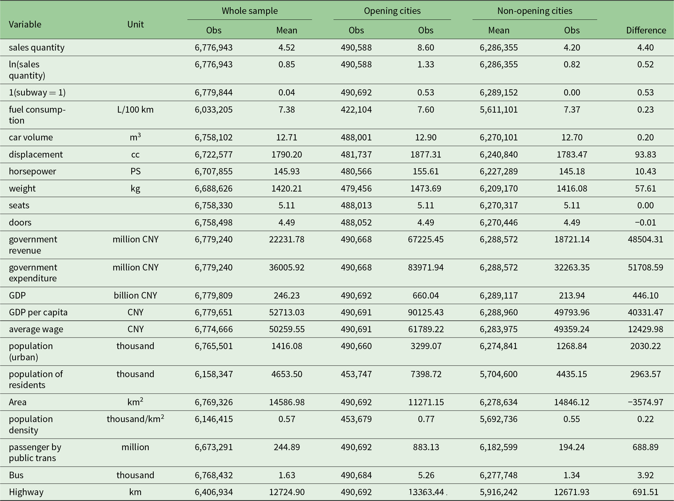
We summarize all the variables involved in our study in table 2 for the whole sample, the opening cities and the non-opening cities. Descriptive analysis shows that there are significantly fewer observations in the opening cities than in the non-opening cities, largely because there are many more non-opening cities than opening cities. Car sales and city characteristics vary across different cities. The sales in the opening cities are significantly higher than those in the non-opening cities. As for the demographic and economic characteristics, the opening cities typically have more government revenue, are significantly more developed, are wealthier and have larger populations. The opening cities also have better traffic systems, featuring a higher number of public transportation passengers, more buses in use and longer lengths of highways. The large differences between the opening cities and the non-opening cities imply that it is necessary to assign weights to the non-opening cities to make the two groups of cities more comparable.
Descriptive analysis of the whole sample, the treatment group and the control group

Notes: This table presents the summary statistics for all the variables involved in our analysis, including car sales, indicators of rail transit opening, car attributes and city characteristics. As explained earlier, the variable fuel consumption is measured in liters per 100 km and is the inverse of fuel economy. The lower the fuel consumption, the higher the fuel economy is. CNY denotes Chinese Yuan.
Figure 1 depicts the trend of the average car sales in the opening cities, in the non-opening cities and in all cities. In each type of cities, car sales exhibit seasonal fluctuations. The sales in the opening cities are about 15 thousand each month, significantly higher than those in the non-opening cities (less than 5 thousand each month).
Average sales in the opening cities, non-opening cities and all cities.

3. Empirical method
3.1. Weights assigning method
As shown in section 2, opening cities differ from non-opening cities in many demographic and economic characteristics, which indicates that car sales in the two groups of cities may not be comparable. To address this problem, we select two groups of comparable cities and assign weights to the non-opening cities. To be more specific, we match the opening cities with non-opening cities using the propensity score matching method (PSM method).Footnote 7 In the regressions that follow, we apply the weights from the PSM method to the observations in the corresponding cities, similar to estimating the average treatment effect in Becker and Ichino (Reference Becker and Ichino2002) and Titus (Reference Titus2007).
When implementing the PSM method, it is important to choose the variables for matching. The matching covariates should satisfy the criterion that, conditional on these covariates, the treatment (which, in our context, is the rail transit openings) is random. In China, cities planning to build rail transit are obliged to submit applications to the State Council and the National Development and Reform Commission (NDRC for short). The State Council and NDRC approve the applications based on four factors: government revenue, GDP, population and passenger volume.Footnote 8
The requirements in the document can be seen as the most essential factors determining whether cities can have rail transit. We match the opening cities with non-opening cities using eight variables based on these factors. The eight variables are government revenue, government expenditure, GDP, GDP per capita, the registered population living in urban areas, passenger volume by public transportation, the number of buses in use and total road length. Government revenue and government expenditure serve as indicators of local governments’ feasible funds, which can support the costly rail transit construction. Although government revenue and government expenditure may not directly relate to car sales, they could be related to other city characteristics, such as economic development, which affects car sales. GDP, GDP per capita and the urban-registered population are emphasized in the document and are also important determinants of travel demand and car demand. Passenger volume, the number of buses and total road length contain information about the local traffic conditions, affecting both travel demand and car demand.
We use the three-year average value of each variable before our sample period started (i.e., the average value for 2010, 2011 and 2012) for matching. The Kernel matching method is adopted since Kernel matching assigns different weights to the non-opening cities according to the ‘distance’ between the non-opening cities and the opening cities. Considering that different PSM settings can produce different combinations of opening and non-opening cities, leading to different estimation results, we examine whether our main results are robust to variable values for different years and to different matching methods. These results are included in table A13 in the online appendix.
We use the probit model to estimate the propensity score and adopt the Epanechnikov kernel function to calculate the weights assigned to the non-opening cities. We only keep the cities whose propensity scores fall in the common support. This setting leaves us with eight opening cities and 215 non-opening cities. Through the PSM process, we obtain two groups of cities for the opening cities and the non-opening cities. Each non-opening city is assigned a weight that indicates its importance in matching an opening city.
After matching, we evaluate the balance of the matching variables between the obtained two groups of cities, i.e., testing the balance assumption. The results of the test are depicted in table 3 (for the graphical result of the test, see figure A1 in the online appendix). Before the matching process, there are significant differences in covariates for the two groups of cities. These differences are largely eliminated after applying PSM. The t-test cannot reject the hypothesis that there are no differences in the eight covariates between the two groups of cities. The balance test informs that the PSM method successfully makes the two selected groups of cities more similar. The range of common support can be found in figure A2 in the online appendix.
Results of the balance test

3.2. Two-way fixed effects panel regression
We employ the two-way fixed effects panel model to estimate the impact of rail transit openings on car sales, similar to Liang and Xi (Reference Liang and Xi2016), Li et al. (Reference Li, Liu, Purevjav and Yang2019) and Zheng et al. (Reference Zheng, Zhang, Sun and Wang2019), which also control for individual fixed effect and time fixed effect in the models. To start with, we first estimate the average effect of rail transit openings on all types of cars using equation (1).Footnote 9 This preliminary estimation can help us understand how rail transit openings influence car sales in general:
 \begin{equation}in({q_{ict}})\, = \,1{(subway = 1)_{ct}}\alpha \, + \,{X_i}\theta \, + \,{\pi _i} \times {\mu _c} \times Yea{r_t}\, + \,Yea{r_t} \times Mont{h_t}\, + \,{\varepsilon _{ict}}\end{equation}
The dependent variable 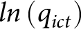 $ln\left( {{q_{ict}}} \right)$ is the logarithm of the sales of car type
 $i$ in city
 $c$ at time
 $t$. The binary variable
 $1{\left( {subway = 1} \right)_{it}}$ is the variable we are most interested in, representing the time after city
 $c$ opened its first rail transit line during 2013–2015. The coefficient
 $\alpha $ indicates to what extent rail transit openings affect the sales of each car type on average. We also distinguish the effect of multiple openings through using a continuous independent variable and using a series of dummy variables. To further quantify the impact of rail transit lines, we replace the dummy variable for rail transit openings with the total length of rail transit lines in the cities. The detailed specifications and the results are provided in the online appendix (tables A5–A10).
We control for car attributes, including fuel-consumption rate, car size (defined by length×width×height), displacement, horsepower, weight, number of seats and number of doors, following Lin and Linn (Reference Lin and Linn2023) and Li (Reference Li2023). The city-model fixed effect 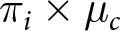 ${\pi _i} \times {\mu _c}$ not only captures local preferences in different cities but also controls for the heterogeneous impact of observed and unobserved characteristics of each car model on car sales in different cities. We include the city-year fixed effect
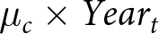 ${\mu _c} \times Yea{r_t}$ to account for all the city-level time-varying factors affecting car sales, including local policies and local demographic features. The year-month fixed effect
 $Yea{r_t} \times Mont{h_t}$ controls for the common time trends in car sales, seasonal fluctuations and nationwide demand shocks (such as tax adjustments and national policies). Since there may be heteroscedasticity with the error term, we adopt robust standard errors when estimating.
We also estimate the baseline specification using staggered difference-in-differences estimators as a robustness check, and delineate the results in table A3 in the online appendix.
To avoid the problem that the high car sales at the end of the year may bias our estimation, we estimate the baseline specification after excluding the two cities which opened the rail transit at the end of the year. The results are shown in tables A11 and A12 in the online appendix.
After we derive the average effect of rail transit openings, we continue to examine the heterogeneous impact of rail transit openings on cars with different fuel-consumption levels. We add an interaction term of  $1{\left( {subway = 1} \right)_{ct}}$ and fuel-consumption level to equation (1) to capture this heterogeneity, and get the following specification:
 \begin{align}
ln\left({{q_{ict}}} \right) &= 1{{\left( {subway = 1} \right)}_{ct}}\alpha + F{C_i} \times 1{{\left( {subway = 1} \right)}_{ct}}\beta + {X_i}\theta\nonumber\\
&\qquad+ {\pi _i} \times {\mu _c} + {\mu _c} \times Yea{r_t} + Yea{r_t} \times Mont{h_t} + {\varepsilon _{ict}}.
\end{align}
This equation can be rewritten as follows:
 \begin{align*}
ln\left( {{q_{ict}}} \right) &= \left( {\alpha + F{C_i}\beta } \right)1{{\left( {subway = 1} \right)}_{ct}} + {X_i}\theta + {\pi _i} \times {\mu _c} + {\mu _c} \times Yea{r_t}\\
&\qquad+ Yea{r_t} \times Mont{h_t} + {\varepsilon _{ict}}.
\end{align*}
The term 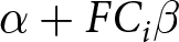 $\alpha + F{C_i}\beta $ can be interpreted as the marginal effect of rail transit openings on the percentage change in sales for cars with fuel consumption
 $F{C_i}$. We assume that the impact of rail transit openings on car sales is a linear function of fuel consumption. We make the hypothesis that rail transit openings have a greater impact (in reducing sales) on low-fuel-consumption cars and less or even no effect on high-fuel-consumption cars. This is because buyers of low-fuel-consumption cars generally have lower incomes and are prone to take rail transit. In contrast, buyers of high-fuel-consumption cars are typically wealthier and tend to keep the option of commuting by car. Therefore, the estimated coefficient
 $\alpha $ is expected to be negative and
 $\beta $ is expected to be positive. In that way, as fuel consumption increases, the impact of rail transit openings on car sales diminishes (recall that
 $FC$ is the inverse of fuel economy). It is possible that at some
 $FC$ value, the impact of openings becomes zero and turns positive above this threshold. The threshold value can be calculated as
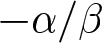 $ - \alpha /\beta $. Rail transit openings decrease car sales within the interval
 $FC \in \left[ {0, - \alpha /\beta } \right]$. This interval can be comprehended as the range of cars, which rail transit can influence. We will also calculate this threshold according to the regression results.
4. Results
4.1. Baseline model
First, we estimate equation (1) to get the average effect of rail transit openings on all types of cars. We estimate three specifications with different sets of controls and fixed effects. The results are shown in table 4. The coefficient  $\alpha $ is significant and negative when controlling for city-model and city-year fixed effects. This indicates that variations in city demographics and car models can confound the effect of rail transit openings and should be controlled for. On average, rail transit openings lead to a decrease of about 2.27 per cent in sales for each type of cars each month after the opening.
Baseline estimations of the impact of rail transit openings on car sales quantity

Notes: The dependent variable is the logarithm form of the sales quantity. The regressions are all run with the PSM weights assigned to cities. The weights employed are computed according to the yearly average value of PSM variables from 2010 to 2012. Car attributes include fuel consumption, size, displacement, horsepower, weight, number of seats and number of doors. Specifications in the three columns are different in the sets of fixed effects. The specification in column (1) includes city fixed effect and year-month fixed effect. The specification in column (2) includes city-year fixed effect and year-month fixed effect. The specification in column (3) includes the city-car model fixed effect, city-year fixed effect and year-month fixed effect. Robust standard errors are in parentheses.
Next, we estimate the heterogeneous effect of rail transit openings on cars with different fuel economy. The estimation results for equation (2) and the corresponding threshold are presented in table 5. Without controlling for city-model and city-year fixed effects, the estimated coefficients for the specification in column (1) are insignificant. After adding the city-model fixed effect and city-year fixed effect,  $\alpha $ is significantly negative and
 $\beta $ is significantly positive for the specification in column (3). This reinforces the need to control for city demographics and car model attributes to avoid confoundedness.
Baseline estimations of the impact of rail transit openings on car sales quantity (using fuel consumption in the interaction term)

Notes: The dependent variable is the logarithm form of the sales quantity. The regressions are all run with the PSM weights assigned to cities. The weights employed are computed according to the yearly average value of PSM variables from 2010 to 2012. Car attributes include fuel consumption, size, displacement, horsepower, weight, number of seats and number of doors. Specifications in the three columns are different in the sets of fixed effects. The specification in column (1) includes city fixed effect and year-month fixed effect. The specification in column (2) includes city-year fixed effect and year-month fixed effect. The specification in column (3) includes the city-car model fixed effect, city-year fixed effect and year-month fixed effect. Robust standard errors are in parentheses.
The values of  $\alpha $ and
 $\beta $ suggest that for a car with the average fuel consumption in our sample (i.e., with the fuel consumption of 7.4 L/100 km), a rail transit line opening leads to a 2.47 per cent decrease in sales (according to the specification in column (3) in table 5), which is comparable to the finding in column (3) in table 4. The signs of
 $\alpha $ and
 $\beta $ indicate that low-fuel-consumption cars experience a greater decline in sales, while high-fuel-consumption cars are less affected. This indicates that the potential buyers of high-fuel-consumption cars are less likely to change their travel mode in response to new rail openings. A possible explanation is that the buyers of high-fuel-consumption cars tend to have higher incomes (considering that high-fuel-consumption cars are typically expensive). In contrast, the buyers of low-fuel-consumption cars often have lower incomes, making them more likely to substitute driving with public transportation. This aligns with the findings in Wang et al. (Reference Wang, Xu and Qin2014), which demonstrated that high-income individuals are more inelastic in driving as a travel decision.
The fuel-consumption thresholds derived from the estimated coefficients are comparable across different control settings. The threshold values in column (2) and column (3) are both above 10 L/100 km, which is a rather high-fuel-consumption level for the cars in our sample. This means that most car types in our sample are estimated to decrease in sales due to rail transit openings. To illustrate the economic implications of the results, we plot the density of fuel-consumption levels for cars in the sample, together with the marginal effect of rail transit openings against fuel-consumption levels (i.e., 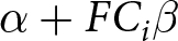 $\alpha + F{C_i}\beta $) in figure A3 in the online appendix. Most cars have fuel-consumption levels (for 100 km) within the interval [5, 10], which makes the overall effect of rail transit openings on car sales negative, as shown in table 4, a 2.27 per cent decrease.
To further confirm our findings about the different substitution patterns among populations, we run another set of regressions with the size (length×width×height) of cars to interact with the rail transit opening dummy as another aspect of car features. The specification and the estimated results are depicted in table A4 in the online appendix.
An implication of our results is that to accurately evaluate the welfare impact of rail transit openings, we need to differentiate the sales changes of various car types. The effect of rail transit on discouraging car sales is stronger on low-fuel-consumption cars, which are more energy-efficient and have less impact on energy consumption and emissions. In contrast, the effect of rail transit is smaller or even positive on high-fuel-consumption cars that consume much more gasoline and emit more pollutants. Our calculations in section 4.4 will present accurate estimates of fuel savings and lifetime carbon emission reductions linked to rail transit openings and highlight which level of fuel-consumption cars contribute the most to the fuel savings.
4.2. The dynamic effects of the rail transit opening
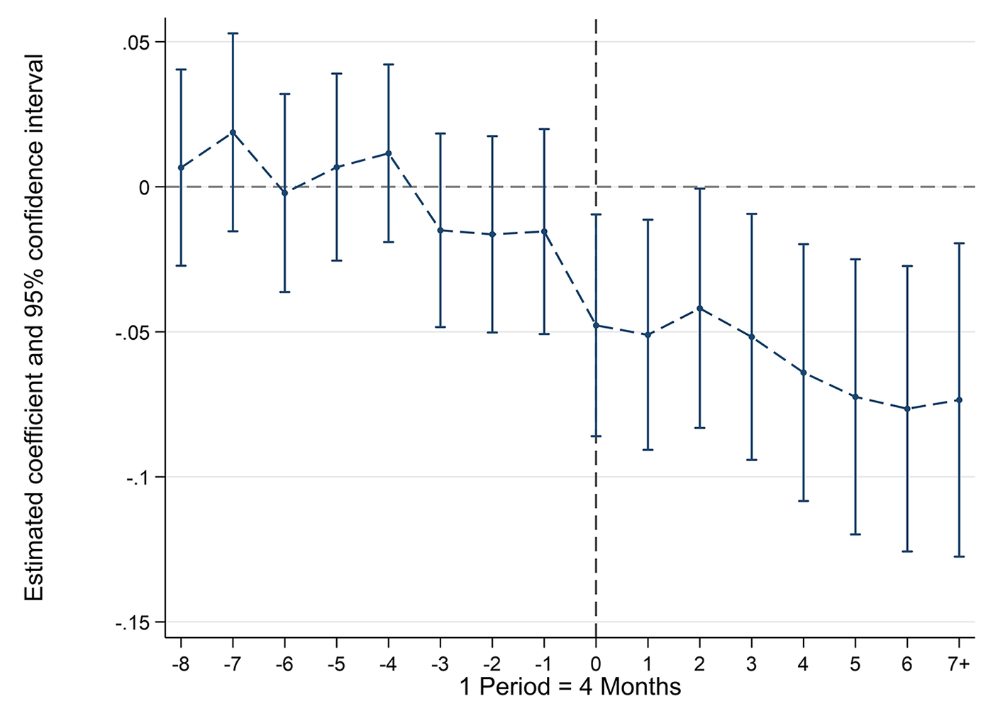
We are also interested in the whole dynamic effect of rail transit openings. Since residents are likely to know about the future opening of a new rail transit line in advance (which is highly possible because the tests of new rail transit lines are usually reported as important news), the effect of rail transit openings may start before the actual opening date. As for the lagged effect of openings, consumers may still cancel their purchasing plans several months after the new rail transit openings, while it is also possible that the impact of rail transit openings dwindles over time. To capture these dynamics, we use a series of dummies for different times before and after the rail transit openings.Footnote 10 We estimate the following specification using the event study framework:
 \begin{equation}
ln\left( {{q_{ict}}} \right) = \mathop \sum \limits_{k = - 8}^7 1{\left( {subway = 1} \right)_{ct,k}}{\beta ^k} + {X_i}\theta + {\pi _i} \times {\mu _c} + {\mu _c} \times Yea{r_t} + Yea{r_t} \times Mont{h_t} + {\varepsilon _{ict}}\,\,\,\,\,\,\,\,\end{equation}
In this specification, the key indicators  $1{\left( {subway = 1} \right)_{ct,k}}$ equal 1 if and only if
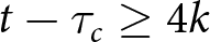 $t - {\tau _c} \geq 4k$ and
 $t - {\tau _c} \leq 4k + 3$, where
 ${\tau _c}$ is the month of the first rail transit opening in city
 $c$ during the sample period (
 $k = 7$ is an exception, where
 $1{\left( {subway = 1} \right)_{ct,k}} = 1$ if and only if
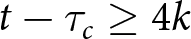 $t - {\tau _c} \geq 4k$). The value of
 $k$ ranges from −8 to 7. The coefficient
 ${\beta ^k}$ represents the average impact of rail transit openings during the period
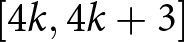 $\left[ {4k,4k + 3} \right]$, compared to the baseline period (
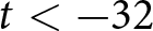 $t \lt -32$). The series of periods covers nearly all the pre-opening and post-opening stages in our sample, helping to reveal a complete picture of the evolving trend. Through comparing the magnitude of a series of
 ${\beta ^k}$, we can understand how the impact changes over time.
The estimation results for the key indicators are plotted in figure 2. This figure indicates that the effect of rail transit occurs after the openings, with a slight and insignificant decline in car sales before the openings. This shows that most consumers adjust their purchase decisions after the openings, and a few consumers may change their purchase plans 1–12 months before the openings. After the openings, there is a lasting impact of rail transit openings. The impact remains significant one year after the openings, with no noticeable decrease in magnitude. This implies that rail transit openings may exert a permanent effect on residents’ car purchase decisions in that city, which provides evidence for the long-run welfare effects of rail transit openings.
The evolvement of the effect of rail transit openings.

4.3. Heterogeneity analyses
It is reasonable to assume that the effect of openings is heterogeneous in different cities. To understand how the effect of rail transit openings varies with the characteristics of cities, we divide the opening cities (after PSM)Footnote 11 into two groups according to GDP, public revenue, residential population, area and number of buses, respectively, and according to whether the cities have rail transit before 2013. Specifically, to take population as an example, we first calculate the average population from 2010 to 2012 for each city and derive the median of these averages. Cities are categorized into the ‘high population’ group if their three-year average population exceeds the median. Otherwise, cities are sorted as ‘low population’. This categorization is conducted for all the variables. In the regressions, we combine each subgroup of categorized opening cities with all the non-opening cities and re-estimate the model specification in column (3) in table 5, which includes the most comprehensive control variables. Table 6 presents the estimation results and the corresponding thresholds.
Heterogeneity analysis of the impact of rail transit openings on car sales quantity

Notes: This table reports the heterogeneity test for rail transit openings’ impact in different cities. The dependent variable is the logarithm form of the sales quantity. The regressions are all run with the PSM weights assigned to cities. The weights employed are computed according to the yearly average value of PSM variables from 2010 to 2012. Car attributes include fuel consumption, size, displacement, horsepower, weight, number of seats and number of doors. The specification in each column includes city-car model fixed effect, city-year fixed effect and year-month fixed effect. Robust standard errors are in parentheses.
In cities without rail transit before 2013, the estimated effect of rail transit openings is larger. This implies that when a city opens rail transit for the first time, many residents choose to forgo car purchases and turn to rail transit. For cities with rail transit before, the opening of a new line has less effect.
In cities with higher GDP, the estimated  $\alpha $ and
 $\beta $ are statistically significant and larger in absolute value. At the average fuel-consumption level of 7.4 L/100 km, car sales in high-GDP cities decrease by about 3.52 per cent, while sales in low-GDP cities decrease by about 1.21 per cent. This suggests that rail transit openings exert a greater negative impact in more developed and wealthier cities. This result seems contrary to our earlier statements and existing literature on car purchases that low-income consumers are more likely to give up car purchases and switch to rail transit. An explanation is that wealthier cities have more residents who can afford to purchase a car and a fraction of them are right on the edge to be affected by rail transit. Also, congestion tends to be severer in wealthier cities, making rail transit more attractive.
In cities with higher government revenue, the effect of rail transit openings is also greater. On the one hand, cities with higher government revenue are typically more economically developed. On the other hand, in these cities, better funding allows for improved rail transit systems, which can attract more passengers to commute by rail transit.
Rail transit openings have a larger impact in cities with bigger populations and larger areas. More populous cities have a greater base number of car sales, which likely contributes to the larger impact of rail transit openings. In larger cities, residents may have a larger demand for cars to travel, if no rail transit is available. When efficient public transportation is available, i.e., a new rail line opens, residents will postpone or cancel car purchases in favour of using public transit.
In cities with more buses, rail transit openings have a smaller impact on car sales. Buses serve as a substitute for rail transit, which weakens the effect of rail transit openings.
4.4. Welfare implications
In this section, we provide a back-of-the-envelope calculation of the welfare gains from the rail transit openings in our sample.
An important welfare improvement from rail transit openings is the gasoline saved by reducing car purchases. Through the identification of the heterogeneous impact of rail transit on cars with different fuel-consumption levels, we can accurately calculate the fuel savings of each car type.
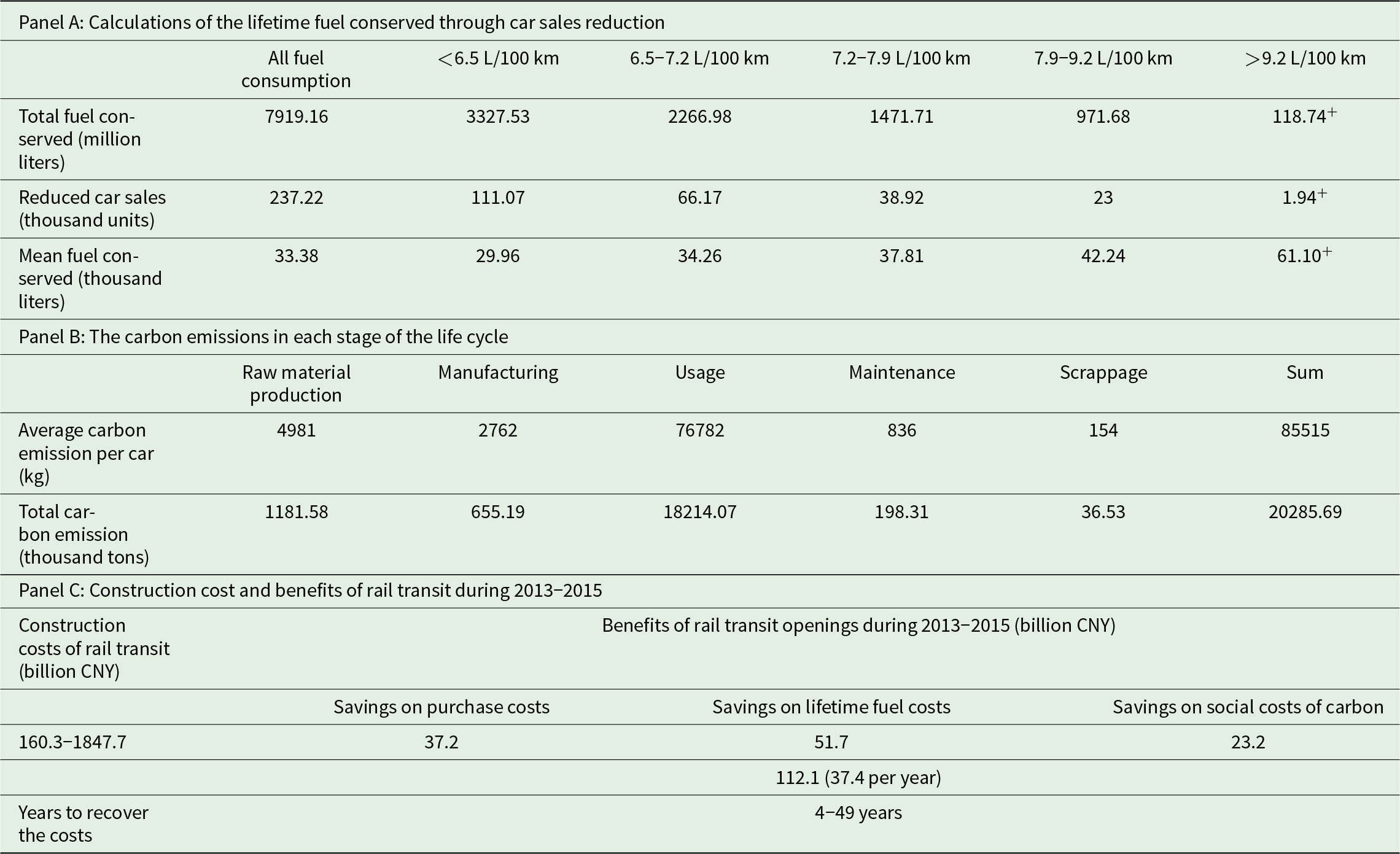
We calculate the gasoline conservation in driving resulting from rail transit openings following the process delineated in the online appendix. We divide all cars equally into five groups according to fuel consumption and calculate the fuel savings in each group to show the main contributors to fuel savings due to rail transit openings. The total fuel savings by rail transit openings together with the fuel conserved in each car group are illustrated in panel A of table 7.
Welfare analyses of rail transit openings

Notes: In each row of panel A, the numbers with no superscript mean that sales of cars in this category decrease so that gasoline is conserved. The numbers with a ‘ +’ superscript mean that in this car category, sales of some types of cars increase, causing more gasoline consumption. Construction costs of rail transit come from the estimates of Baum-Snow and Kahn (Reference Baum-Snow and Kahn2005): $25–$287 million per mile (about 0.104 billion CNY per km to 1.199 billion CNY per km). The savings on lifetime fuel costs are computed using the average gasoline price after 2013, approximately 6.53 CNY/L. The social cost of carbon is derived from Rennert et al. (Reference Rennert, Errickson, Prest, Rennels, Newell, Pizer, Kingdon, Wingenroth, Cooke, Parthum, Smith, Cromar, Diaz, Moore, Müller, Plevin, Raftery, Ševčíková, Sheets, Stock, Tan, Watson, Wong and Anthoff2022), i.e., $185 per tCO2.
During the sample period, approximately 7.9 billion liters of gasoline for driving is saved from reduced car ownership due to rail transit openings. The cars in the group ‘<6.5°L/100 km’ are the main contributors to fuel savings, accounting for more than one-third of the total fuel conserved. Although the average fuel conserved per car type in the ‘<6.5°L/100 km’ group is relatively small because of their low-fuel-consumption level, this group contains the most prevalently sold car types. As a result, the reduction in sales for this group is the largest, leading to the largest total fuel conservation. For the groups ‘6.5–7.2°L/100 km’, ‘7.2–7.9°L/100 km’ and ‘7.9–9.2°L/100 km’, the large average fuel savings are offset by the smaller impact of rail transit openings on their sales. Car models in the group ‘>9.2°L/100 km’ do not contribute to the gasoline savings according to our calculations, since their sales did not decrease with rail transit openings.
Another important aspect of welfare improvement is the reduction in carbon emissions related to decreased car sales, especially in the context of global warming. The calculation method for the total reduction in carbon emissions is included in the online appendix. The carbon emissions in each stage of a car's life cycle are presented in panel B of table 7. The total reduction in carbon emissions due to decreased car sales is around 20.3 million tons. The carbon emissions from driving account for up to 89 per cent of the total carbon emissions. This result shows that through the decrease in car sales, rail transit openings reduce the carbon emissions related to all the stages in a car's life cycle, especially in driving.
Considering that rail transit construction is very expensive, we further compare the benefits of rail transit openings with the construction costs of rail transit lines opened during our sample period. The details of the calculation of the costs and benefits are shown in the online appendix. The estimated costs and benefits of rail transit openings are delineated in panel C of table 7. The total estimated benefits of rail transit openings during 2013–2015 are about 112.1 billion CNY, i.e., 37.4 billion CNY/year. However, rail transit can still influence consumers’ car purchase behaviour after the sample period. This means that after 2015, the opened rail transit lines will continue to discourage car sales and generate benefits. Assuming that the rail transit openings produce the benefits of 37.3 billion CNY/year, it will take about 4–49 years to recover the construction costs, which is a modest operation time for rail transit.
These calculations imply that the welfare gains from rail transit expansion are substantial. However, this is only part of the long-run impact of rail transit through discouraging car ownership. Other impacts, such as resource conservation during the car production process, long-run improvements in air quality and reduced road congestion, are not quantified in this paper. Our results provide insights into evaluating the benefits of rail transit investment. Our study also points out the main contributors to fuel savings. Though low-fuel-consumption cars consume less fuel in driving, they are the most affected type of cars when a new rail transit line opens. The significant decrease in their sales makes them a key driver of fuel savings.
5. Conclusions
This paper investigates the impact of rail transit openings on car sales in Chinese cities. By differentiating the effects for cars with different fuel economy, we reveal the heterogeneous travel substitution patterns among the buyers of different types of cars. Our results indicate that rail transit openings discourage car purchases, with a larger reduction in sales for low-fuel-consumption cars, while the effect is negligible for high-fuel-consumption cars. This implies that the consumers of more fuel-efficient cars have a larger substitution elasticity between taking rail transit and driving private cars. This highlights the different travel substitution patterns among the population. Moreover, our heterogeneity analyses show that residents are more likely to substitute driving with rail transit in cities that open rail transit for the first time and which have more developed economies, higher government revenue, larger populations, bigger areas and fewer buses. Welfare calculations indicate that approximately 7.9 billion liters of gasoline and 20.3 million tons of carbon emissions are saved due to rail transit opening during our sample period. It will take about 4–49 years for the benefits of rail transit openings to cover their construction costs. This suggests significant welfare improvements resulting from rail transit openings, especially considering the long-run impact.
Our study suggests that rail transit openings have a long-run impact on travel decisions, further leading to long-run changes in congestion levels, air quality and resource consumption. This long-term impact through discouraging car purchases is rarely documented in existing literature, and the current evaluation of rail transit's welfare improvements may be underestimated. Our results imply that rail transit investments could be more beneficial than expected. It will take 4–49 years for the benefits of rail transit to recover the immense construction costs. This finding justifies the large investments in rail transit programs in China.
However, this study is not without limitations. We list the limitations below and discuss several future research directions in the online appendix. First, we lack city-level data related to transportation, such as subway passenger volume, bus passenger volume or traffic congestion indexes. Combining these data with our research could reveal the specific transportation substitution patterns among residents, which we will explore further. Second, other potential benefits from car sales reduction remain to be examined, such as resource conservation, air quality improvements and congestion alleviation. Third, we do not include more variables in the PSM process, such as the transportation data, car portfolios and the spatial structure of the city, due to the data availability. Although the results may not be affected, it is better to include more variables for more accurate matching if the data become available.
Supplementary material
The supplementary material for this article can be found at https://doi.org/10.1017/S1355770X25000191.
Funding statement
We are grateful to the computational supports provided by the Public Computing Cloud at Renmin University of China. We gratefully acknowledge the National Natural Science Foundation of China (Grant Nos 72173126, 72272145, 72134006 and 72361167635) and Singapore Ministry of Education (Tier 1 Grant No. A-8001876-00-00).
Competing interests
The authors declare none.