1 Introduction
Bifurcations in piping configurations are ubiquitous elements in many aspects of fluid flows. Among man-made constructions, pipe bifurcations are common in water, steam and other fluid distribution systems within buildings, structures and industry. The use of pipe bifurcations in microfluidic channels for thermal management is also common (e.g. Senn & Poulikakos Reference Senn and Poulikakos2004; Kockmann et al. Reference Kockmann, Engler, Haller and Woias2005; Haller, Woias & Kockmann Reference Haller, Woias and Kockmann2009). Not surprisingly, bifurcating pipe flow is by no means restricted to man-made systems. The pulmonary artery, which distributes deoxygenated blood from the right ventricle of the heart to the lungs for oxygenation, is a T-shaped pipe bifurcation similar to the geometry we discuss in this article. Likewise, the basilar artery splits into two vertebral arteries underneath the brain, supplying the brain with oxygen.
The shape of the pipe bifurcation can be characterised by the angle between the inlet and outlet pipes. In this article, we refer to bifurcations as arrow-, T- and Y-junctions, based on the shape of the configuration. The ‘impacting’ configuration has a single inlet (e.g. at the bottom of a ‘T’ shape) and two symmetric outlets (e.g. the sides of the ‘T’); such a configuration is the subject of this study. In contrast, the ‘mixing’ configuration describes the reverse flow, with two inlets and one outlet (e.g. Engler et al.
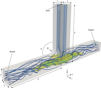
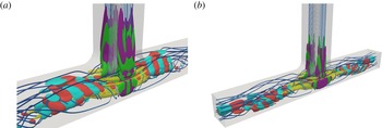
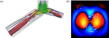
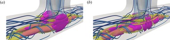
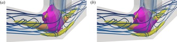
Reference Engler, Kockmann, Kiefer and Woias2004; Bothe, Stemich & Warnecke Reference Bothe, Stemich and Warnecke2006; Dreher, Kockmann & Woias Reference Dreher, Kockmann and Woias2009). Figure 1 shows the impacting flow through a
 $\unicode[STIX]{x1D703}=90^{\circ }$
T-junction, with
 $\unicode[STIX]{x1D703}$
indicating the junction angle.
The base flow for
 $\unicode[STIX]{x1D703}=90^{\circ }$
and
 $Re=560$
, shown as velocity streamlines (blue, low speed; grey, high speed), an additional set of streamlines (cyan) highlighting recirculation arising from vortex breakdown and a single level set (yellow) of
 $Q$
. The fluid flows from the top and exits at the two sides. The junction corner radius of curvature is
 $R=0.4$
.

The key feature of pipe bifurcation flows is the occurrence of vortex breakdown at up to four locations in the junction. Vigolo, Radl & Stone (Reference Vigolo, Radl and Stone2014) first reported this phenomenon in both a bubble-laden flow experiment and a single-phase computation when the Reynolds number
 $Re$
, based on the pipe width and the average inlet flow speed, exceeds 350. In this laminar flow regime, the junction walls curve streamlines from the inlet and induce large vortex pairs aligned with the outlets. The vortices can be identified with
 $Q$
-contours, where if
 $\boldsymbol{u}$
is the velocity field,
 $\unicode[STIX]{x1D64E}=(\unicode[STIX]{x1D735}\boldsymbol{u}+(\unicode[STIX]{x1D735}\boldsymbol{u})^{\text{T}})/2$
is the rate of strain tensor,
 $\unicode[STIX]{x1D734}=(\unicode[STIX]{x1D735}\boldsymbol{u}-(\unicode[STIX]{x1D735}\boldsymbol{u})^{\text{T}})/2$
is the rotation tensor and
 $\Vert \cdot \Vert _{F}$
is the Frobenius norm, then
 $Q:=(\Vert \unicode[STIX]{x1D734}\Vert _{F}^{2}-\Vert \unicode[STIX]{x1D64E}\Vert _{F}^{2})/2$
(see Chakraborty, Balachandar & Adrian (Reference Chakraborty, Balachandar and Adrian2005) and Haller (Reference Haller2005) for discussions of vortex identification schemes). Figure 1 shows a T-junction flow at
 $Re=560$
, using streamlines and a single level set of
 $Q$
to visualise the three-dimensional flow. The creation of the large vortices by the junction geometry is similar, in principle, to the way in which centrifugal forces create vortices in the fully developed Dean flow through a slowly bending pipe (see, e.g., Winters Reference Winters1987).
Unlike Dean flow, however, the intrinsically three-dimensional breakdown of the pipe bifurcation vortices creates recirculation regions internal to the flow where bubbles or low-density particles that are suspended in the flow may become trapped (Vigolo et al. Reference Vigolo, Radl and Stone2014). We note that previous authors (e.g. Karino et al. Reference Karino, Goldsmith, Motomiya, Mabuchi and Sohara1987; Senn & Poulikakos Reference Senn and Poulikakos2004; Kockmann et al. Reference Kockmann, Engler, Haller and Woias2005; Doorly & Sherwin Reference Doorly and Sherwin2009; Haller et al. Reference Haller, Woias and Kockmann2009) have not mentioned the existence of vortex breakdown in T-junction flow, which is the most studied of the three junction shapes. The topic of vortex breakdown has seen much coverage and debate in the fluid dynamics literature, with many attempting to explain the genesis of this phenomenon. The articles by Hall (Reference Hall1972), Leibovich (Reference Leibovich1978), Leibovich (Reference Leibovich1984), Brown & Lopez (Reference Brown and Lopez1990), Lopez (Reference Lopez1990), Lopez & Perry (Reference Lopez and Perry1992), Lucca-Negro & O’Doherty (Reference Lucca-Negro and O’Doherty2001) and many others review the phenomenology of vortex breakdown, as well as prevailing theories for its formation. In the language of Leibovich (Reference Leibovich1978), the vortex breakdown we observe in pipe bifurcations is similar to a ‘near-axisymmetric’ or ‘bubble-like’ breakdown. That is, interior stagnation points mark the sudden beginning or end of a nearly axisymmetric envelope comprising the region of swirling recirculation.
The stability analysis of vortex breakdown has been a topic of research in recent years. For example, Gallaire et al. (Reference Gallaire, Ruith, Meiburg, Chomaz and Huerre2006) examined an axisymmetric swirling jet undergoing ‘spiral’ vortex breakdown, where a streakline in the vortex core would experience a sudden kink, followed by a corkscrew twisting. They found the spiral breakdown to be the result of a nonlinear global mode, itself precipitated by absolute instability in a base state with axisymmetric vortex breakdown. Oberleithner et al. (Reference Oberleithner, Sieber, Nayeri, Paschereit, Petz, Hege, Noack and Wygnanski2011), Meliga, Gallaire & Chomaz (Reference Meliga, Gallaire and Chomaz2012) and Qadri, Mistry & Juniper (Reference Qadri, Mistry and Juniper2013) similarly studied global modes of the vortex breakdown in an axisymmetric swirling jet.
The stability of vortex structures is a common topic in the flow instability literature, for which a complete review would not be possible here. Besides the aforementioned studies in vortex breakdown, research in vortex stability has covered idealised flow configurations such as the single free vortex (see, e.g. Pierrehumbert Reference Pierrehumbert1986; Loiseleux, Chomaz & Huerre Reference Loiseleux, Chomaz and Huerre1998; Loiseleux, Delbende & Huerre Reference Loiseleux, Delbende and Huerre2000; Olendraru & Sellier Reference Olendraru and Sellier2002; Heaton, Nichols & Schmid Reference Heaton, Nichols and Schmid2009), the single vortex with an external strain field (e.g. Eloy & Le Dizès Reference Eloy and Le Dizès1999), the free vortex pair (e.g. Crow Reference Crow1970; Leweke & Williamson Reference Leweke and Williamson1998; Le Dizès & Laporte Reference Le Dizès and Laporte2002) and many other topics. The vast majority of these studies rely on simplifications involving local instability assumptions, or symmetry or invariance in certain spatial dimensions. Over the last decade or so, computational power has improved sufficiently to allow eigendecompositions of high-dimensional linearised flow operators. It is this linear global instability theory that we pursue in this article. In this methodology (Chomaz Reference Chomaz2005), we make no direct assumptions about symmetry or invariance, and we directly compute numerical approximations of the direct and adjoint eigenmodes of the linearised Navier–Stokes operator.
An additional benefit of the eigenmode approach is the ability to compute sensitivities of the linearised Navier–Stokes operator to various perturbations. The sensitivity to spatially localised feedback (Giannetti & Luchini Reference Giannetti and Luchini2007) measures the change in linearisation eigenvalues as a result of infinitesimal point feedback forcing. Such a point forcing is essentially a proportional feedback flow control with a collocated actuator and sensor. Semantically, this sensitivity is often known as the ‘structural sensitivity’, the region of which is called the ‘instability core’ and is closely related to the ‘wavemaker’ born out of a local stability analysis. The sensitivity to base flow modifications (Marquet, Sipp & Jacquin Reference Marquet, Sipp and Jacquin2008), on the other hand, measures the change in linearisation eigenvalues upon altering the flow field about which the Navier–Stokes equation is linearised. Such a sensitivity was first explored by Hill (Reference Hill1992) and Bottaro, Corbett & Luchini (Reference Bottaro, Corbett and Luchini2003). The closely related sensitivity to a steady force (Marquet et al. Reference Marquet, Sipp and Jacquin2008) determines eigenvalue shifts from the introduction of a time-independent force. Such a force could be, for instance, from passive flow control or steady open-loop active flow control.
Continuing from the studies of Gallaire et al. (Reference Gallaire, Ruith, Meiburg, Chomaz and Huerre2006), Oberleithner et al. (Reference Oberleithner, Sieber, Nayeri, Paschereit, Petz, Hege, Noack and Wygnanski2011), Meliga et al. (Reference Meliga, Gallaire and Chomaz2012) and others, Qadri et al. (Reference Qadri, Mistry and Juniper2013) computed the most unstable direct and adjoint eigenmodes of an axisymmetric spiralling jet undergoing vortex breakdown, as well as the sensitivity to spatially localised feedback. These authors found that the most unstable direct eigenmode is largest in the region comprising the wake of the vortex breakdown bubble, and the corresponding adjoint eigenmode is large only in a small region upstream of the bubble. The sensitivity to spatially localised feedback, on the other hand, is largest in a small region that begins slightly upstream of the recirculation bubble, and extends partway into the bubble. Previously, Oberleithner et al. (Reference Oberleithner, Sieber, Nayeri, Paschereit, Petz, Hege, Noack and Wygnanski2011) used experimental data to locate the wavemaker only upstream of the recirculation bubble. The discrepancy between Oberleithner et al.’s and Qadri et al.’s wavemaker locations is a result of the former’s use of a local stability analysis, which is arguably less accurate.
In a study with geometric similarity to our work, Fani, Camarri & Salvetti (Reference Fani, Camarri and Salvetti2013) computed the global stability and sensitivity of a ‘mixing’ T-junction, in which the sides of the ‘T’ are inlets and the bottom of the ‘T’ is a single outlet. They similarly located a direct mode downstream of the junction and an adjoint mode upstream, as expected from the convective nature of the linearised Navier–Stokes equation. Furthermore, the instability core resides in the recirculation regions of the flow. Lashgari et al. (Reference Lashgari, Tammisola, Citro, Juniper and Brandt2014) reported similar results using a three-dimensional stability analysis of the two-dimensional flow through an X-shaped channel junction. These aforementioned studies qualitatively agree with what we report here for the reverse-direction (i.e. ‘impacting’) T-junction flow, with some minor differences. Haward et al. (Reference Haward, Poole, Alves, Oliveira, Goldenfeld and Shen2016) also studied the nature of a pitchfork bifurcation yielding a single spiral vortex in the cross-slot flow, in a configuration similar to the X-shaped junction.
We recently studied T-junction flow numerically, focusing specifically on the coincidence between vortex breakdown bubbles and sensitivity to spatially localised feedback (Chen, Rowley & Stone Reference Chen, Rowley and Stone2015). In this work, we also investigated the nature of the recirculation streamlines, and we briefly described the lack of an appreciable effect from the T-junction corners on the sensitivity of the flow. We also concurrently studied bubble- and particle-laden flows in junctions of angle
 $30^{\circ }\leqslant \unicode[STIX]{x1D703}\leqslant 120^{\circ }$
(Ault et al.
Reference Ault, Fani, Chen, Shin, Gallaire and Stone2016). Through a combination of experiments and simulations, we empirically showed that the presence of vortex breakdown in the single-phase flow is a necessary condition for the capturing and trapping of bubbles and particles in pipe bifurcation flows. Finally, we have separately examined the transition of single-phase flows from curved to straight pipes, using a combination of scaling arguments and numerical simulations (Ault, Chen & Stone Reference Ault, Chen and Stone2015).
In this article, we provide a more complete treatise of impacting pipe bifurcation flows, highlighting the
 $\unicode[STIX]{x1D703}=70^{\circ }$
,
 $90^{\circ }$
and
 $110^{\circ }$
geometries, and we describe their stability and sensitivity analyses. First, in § 2, we review the theories of linear global stability and sensitivity. Next, in § 3, we discuss the nature of the steady-state solutions at varying junction angles and Reynolds numbers. For the
 $90^{\circ }$
T-junction, we describe the flow at
 $Re=320$
, near the onset of vortex breakdown, as well as the flow near the first Hopf bifurcation at
 $Re=556$
. For the
 $70^{\circ }$
arrow-junction and the
 $110^{\circ }$
Y-junction, we first describe supercritical pitchfork bifurcations leading to stable asymmetric steady states at
 $Re=168$
for
 $70^{\circ }$
and 649 for
 $110^{\circ }$
, before these states undergo Hopf bifurcations at
 $Re=200$
and 699 respectively. Next, in § 4, we describe the linear direct and adjoint global modes for these base flows, and indicate specific regions of the geometry where stability and receptivity mechanisms act. In § 5, we also demonstrate that the regions of circulation, sensitivity to spatially localised feedback and sensitivity to base flow modifications largely coincide. We specifically show the effects of localised feedback and base flow modifications on eigenvalue growth rates and frequencies. Finally, we highlight regions where the production and transport of flow perturbations by base flow modifications contribute to the base flow sensitivity. The mesh, boundary conditions, algorithms and software are discussed in appendix A.
2 Linear global stability and sensitivity
2.1 Nonlinear and linearised flow operators
In this section, we review the linear theory of global stability and sensitivity that we apply to the Navier–Stokes equation. Much of this theory can be found in the works by Schmid & Henningson (Reference Schmid and Henningson2001, chap. 7.6.3), Chomaz (Reference Chomaz2005) and Giannetti & Luchini (Reference Giannetti and Luchini2007).
We begin by considering a flow with constant density
 $\unicode[STIX]{x1D70C}$
and constant viscosity
 $\unicode[STIX]{x1D707}$
. Given a characteristic flow speed
 $U$
and geometrical length scale
 $L$
, which we will later specify, we define the Reynolds number
 $Re=\unicode[STIX]{x1D70C}UL/\unicode[STIX]{x1D707}$
. Let
 ${\mathcal{U}}$
denote the space of non-dimensional divergence-free velocity fields, and let
 ${\mathcal{P}}$
denote the space of non-dimensional pressure fields. Choosing the non-dimensional
 $\boldsymbol{x}$
to reside in some spatial domain
 $\unicode[STIX]{x1D6FA}\subset \mathbb{R}^{3}$
, we consider velocity fields
 $\boldsymbol{u}(\boldsymbol{x},t)$
and pressure fields
 $p(\boldsymbol{x},t)$
evolving over non-dimensional time
 $t$
, such that
 $\boldsymbol{u}(\cdot ,t_{0})\in {\mathcal{U}}$
and
 $p(\cdot ,t_{0})\in {\mathcal{P}}$
at each time instant
 $t_{0}$
. We can define the Navier–Stokes operator
 $\mathscr{N}:{\mathcal{U}}\rightarrow {\mathcal{U}}$
by
 $$\begin{eqnarray}\displaystyle \mathscr{N}(\boldsymbol{u}):=-\boldsymbol{u}\boldsymbol{\cdot }\unicode[STIX]{x1D735}\boldsymbol{u}-\unicode[STIX]{x1D735}p+\frac{1}{Re}\unicode[STIX]{x1D6FB}^{2}\boldsymbol{u}, & & \displaystyle\end{eqnarray}$$
where
 $p\in {\mathcal{P}}$
is chosen so that
 $\unicode[STIX]{x1D735}\boldsymbol{\cdot }\mathscr{N}(\boldsymbol{u})=0$
. In addition, one requires appropriate boundary conditions on
 $\boldsymbol{u}$
and
 $p$
, and these are discussed in § A.2. The Navier–Stokes equation then prescribes how a velocity field
 $\boldsymbol{u}(\boldsymbol{x},t)$
evolves in time, and is given by
 $$\begin{eqnarray}\displaystyle \frac{\unicode[STIX]{x2202}\boldsymbol{u}}{\unicode[STIX]{x2202}t}=\mathscr{N}(\boldsymbol{u}). & & \displaystyle\end{eqnarray}$$
A velocity field
 $\boldsymbol{u}_{0}\in {\mathcal{U}}$
, along with its associated pressure field
 $p_{0}\in {\mathcal{P}}$
, is an equilibrium or steady-state solution of (2.2) if
 $\mathscr{N}(\boldsymbol{u}_{0})=\mathbf{0}$
.
The velocity and pressure fields can be written as the perturbations
 $\boldsymbol{u}^{\prime }(\boldsymbol{x},t):=\boldsymbol{u}(\boldsymbol{x},t)-\boldsymbol{u}_{0}(\boldsymbol{x})$
and
 $p^{\prime }(\boldsymbol{x},t):=p(\boldsymbol{x},t)-p_{0}(\boldsymbol{x})$
. The linearisation of
 $\mathscr{N}$
about an equilibrium
 $\boldsymbol{u}_{0}$
yields the linearised Navier–Stokes operator
 $\mathscr{L}:{\mathcal{U}}\rightarrow {\mathcal{U}}$
, given by
 $$\begin{eqnarray}\displaystyle \mathscr{L}\boldsymbol{u}^{\prime }:=-\boldsymbol{u}^{\prime }\boldsymbol{\cdot }\unicode[STIX]{x1D735}\boldsymbol{u}_{0}-\boldsymbol{u}_{0}\boldsymbol{\cdot }\unicode[STIX]{x1D735}\boldsymbol{u}^{\prime }-\unicode[STIX]{x1D735}p^{\prime }+\frac{1}{Re}\unicode[STIX]{x1D6FB}^{2}\boldsymbol{u}^{\prime }, & & \displaystyle\end{eqnarray}$$
where the continuity condition
 $\unicode[STIX]{x1D735}\boldsymbol{\cdot }(\mathscr{L}\boldsymbol{u}^{\prime })=0$
again determines the pressure field
 $p^{\prime }\in {\mathcal{P}}$
. The linearised problem typically has homogeneous boundary conditions since
 $\boldsymbol{u}$
and
 $\boldsymbol{u}_{0}$
generally have the same boundary conditions, as do
 $p$
and
 $p_{0}$
. With these conditions, the linearised Navier–Stokes equation is
 $$\begin{eqnarray}\displaystyle \frac{\unicode[STIX]{x2202}\boldsymbol{u}^{\prime }}{\unicode[STIX]{x2202}t}=\mathscr{L}\boldsymbol{u}^{\prime }. & & \displaystyle\end{eqnarray}$$
For the purpose of the stability analysis, it is also helpful to define an adjoint linearised Navier–Stokes operator. We first choose a complex inner product on the space
 ${\mathcal{U}}$
. For
 $\boldsymbol{u}_{1},\boldsymbol{u}_{2}\in {\mathcal{U}}$
, we define
 $$\begin{eqnarray}\displaystyle \langle \boldsymbol{u}_{1},\boldsymbol{u}_{2}\rangle :=\iiint _{\unicode[STIX]{x1D6FA}}\boldsymbol{u}_{1}(\boldsymbol{x})\boldsymbol{\cdot }\overline{\boldsymbol{u}}_{2}(\boldsymbol{x})\,\text{d}V, & & \displaystyle\end{eqnarray}$$
where
 $\overline{(\cdot )}$
denotes complex conjugation. It should be noted that while the actual velocity field is of course real, we allow for complex velocities because we will be considering complex eigenfunctions of
 $\mathscr{L}$
. Denoting the adjoint velocity field by
 $\hat{\boldsymbol{u}}\in {\mathcal{U}}$
, the adjoint linearised Navier–Stokes operator
 $\mathscr{L}^{\ast }:{\mathcal{U}}\rightarrow {\mathcal{U}}$
is given by
 $$\begin{eqnarray}\displaystyle \mathscr{L}^{\ast }\hat{\boldsymbol{u}}:=-(\unicode[STIX]{x1D735}\boldsymbol{u}_{0})\boldsymbol{\cdot }\hat{\boldsymbol{u}}+\boldsymbol{u}_{0}\boldsymbol{\cdot }\unicode[STIX]{x1D735}\hat{\boldsymbol{u}}-\unicode[STIX]{x1D735}\hat{p}+\frac{1}{Re}\unicode[STIX]{x1D6FB}^{2}\hat{\boldsymbol{u}}. & & \displaystyle\end{eqnarray}$$
To clarify the notation,
 $((\unicode[STIX]{x1D735}\boldsymbol{u})\boldsymbol{\cdot }\boldsymbol{v})_{i}:=\sum _{j}(\unicode[STIX]{x2202}u_{j}/\unicode[STIX]{x2202}x_{i})v_{j}$
. As before, the adjoint pressure
 $\hat{p}\in {\mathcal{P}}$
is determined from the incompressibility condition
 $\unicode[STIX]{x1D735}\boldsymbol{\cdot }(\mathscr{L}^{\ast }\hat{\boldsymbol{u}})=0$
.
In addition, the adjoint problem must satisfy its own boundary condition. Defining
 $$\begin{eqnarray}\displaystyle \boldsymbol{J}:=-(\boldsymbol{u}^{\prime }\boldsymbol{\cdot }\bar{\hat{\boldsymbol{u}}})\boldsymbol{u}_{0}-p^{\prime }\bar{\hat{\boldsymbol{u}}}+\bar{\hat{p}}\boldsymbol{u}^{\prime }+{\displaystyle \frac{1}{Re}}((\unicode[STIX]{x1D735}\boldsymbol{u}^{\prime })\boldsymbol{\cdot }\bar{\hat{\boldsymbol{u}}}-(\unicode[STIX]{x1D735}\bar{\hat{\boldsymbol{u}}})\boldsymbol{\cdot }\boldsymbol{u}^{\prime }), & & \displaystyle\end{eqnarray}$$
the boundary condition is
 $$\begin{eqnarray}\displaystyle \boldsymbol{J}\boldsymbol{\cdot }\boldsymbol{n}=0\quad \text{on }\unicode[STIX]{x2202}\unicode[STIX]{x1D6FA}, & & \displaystyle\end{eqnarray}$$
where
 $\boldsymbol{n}$
denotes the unit outward normal vector. To show this, one readily verifies that
 $$\begin{eqnarray}\displaystyle \unicode[STIX]{x1D735}\boldsymbol{\cdot }\boldsymbol{J}=(\mathscr{L}\boldsymbol{u}^{\prime })\boldsymbol{\cdot }\bar{\hat{\boldsymbol{u}}}-\boldsymbol{u}^{\prime }\boldsymbol{\cdot }\mathscr{L}^{\ast }\bar{\hat{\boldsymbol{u}}}; & & \displaystyle\end{eqnarray}$$
integrating over
 $\unicode[STIX]{x1D6FA}$
, the divergence theorem gives
 $$\begin{eqnarray}\displaystyle \unicode[STIX]{x0222F}_{\unicode[STIX]{x2202}\unicode[STIX]{x1D6FA}}\boldsymbol{J}\boldsymbol{\cdot }\boldsymbol{n}\,\text{d}S=\langle \mathscr{L}\boldsymbol{u}^{\prime },\hat{\boldsymbol{u}}\rangle -\langle \boldsymbol{u}^{\prime },\mathscr{L}^{\ast }\hat{\boldsymbol{u}}\rangle . & & \displaystyle\end{eqnarray}$$
Thus, when the boundary conditions (2.8) are satisfied, the adjoint relation
 $\langle \mathscr{L}\boldsymbol{u}^{\prime },\hat{\boldsymbol{u}}\rangle =\langle \boldsymbol{u}^{\prime },\mathscr{L}^{\ast }\hat{\boldsymbol{u}}\rangle$
holds. It should be noted that (2.8) typically simplifies somewhat, since the boundary conditions on
 $\mathscr{L}$
may make certain terms in (2.7) vanish. The adjoint linearised Navier–Stokes equation is then given by
 $$\begin{eqnarray}\displaystyle \frac{\unicode[STIX]{x2202}\hat{\boldsymbol{u}}}{\unicode[STIX]{x2202}t}=\mathscr{L}^{\ast }\hat{\boldsymbol{u}}. & & \displaystyle\end{eqnarray}$$
2.2 Eigendecomposition
We may now consider the eigendecomposition of the linearised Navier–Stokes operator (2.3). Given some eigenvalue
 $\unicode[STIX]{x1D706}_{j}\in \mathbb{C}$
, the corresponding direct eigenmode
 $\unicode[STIX]{x1D753}_{j}\in {\mathcal{U}}$
satisfies
 $\mathscr{L}\unicode[STIX]{x1D753}_{j}=\unicode[STIX]{x1D706}_{j}\unicode[STIX]{x1D753}_{j}$
. These eigenvalues and eigenmodes yield the long-time behaviour of the linearised dynamics. The direct eigenmode corresponding to the most unstable eigenvalue will dominate the linearised dynamics in the infinite time horizon. Furthermore, when an eigenvalue moves in the complex plane from the stable left half to the unstable right half, the corresponding centre eigenmode plays an important role in characterising the local bifurcation and the resulting centre manifold dynamics (Guckenheimer & Holmes Reference Guckenheimer and Holmes1983, chap. 3).
For the same eigenvalue
 $\unicode[STIX]{x1D706}_{j}$
, the corresponding adjoint eigenmode
 $\unicode[STIX]{x1D74D}_{j}\in {\mathcal{U}}$
satisfies
 $\mathscr{L}^{\ast }\unicode[STIX]{x1D74D}_{j}=\bar{\unicode[STIX]{x1D706}}_{j}\unicode[STIX]{x1D74D}_{j}$
. These adjoint eigenmodes are important in assessing the receptivity of the linear operator to initial conditions and external forcing (see, e.g., Schmid & Henningson Reference Schmid and Henningson2001; Chomaz Reference Chomaz2005; Giannetti & Luchini Reference Giannetti and Luchini2007). This feature can be understood if we introduce an external forcing
 $\boldsymbol{f}(\boldsymbol{x},t)$
in the linearised dynamics; that is,
 $$\begin{eqnarray}\displaystyle \frac{\unicode[STIX]{x2202}\boldsymbol{u}^{\prime }}{\unicode[STIX]{x2202}t}=\mathscr{L}\boldsymbol{u}^{\prime }+\boldsymbol{f}. & & \displaystyle\end{eqnarray}$$
If we assume that
 $\mathscr{L}$
has a full set of eigenvectors
 $\unicode[STIX]{x1D753}_{j}$
, then the solution to this differential equation can be expressed as
 $$\begin{eqnarray}\displaystyle \boldsymbol{u}^{\prime }(\boldsymbol{x},t)=\mathop{\sum }_{j}a_{j}(t)\unicode[STIX]{x1D753}_{j}(\boldsymbol{x}), & & \displaystyle\end{eqnarray}$$
where the coefficients
 $a_{j}(t)$
are governed by
 $$\begin{eqnarray}\displaystyle \frac{\text{d}a_{j}}{\text{d}t}=\unicode[STIX]{x1D706}_{j}a_{j}+\frac{\langle \,\boldsymbol{f},\unicode[STIX]{x1D74D}_{j}\rangle }{\langle \unicode[STIX]{x1D753}_{j},\unicode[STIX]{x1D74D}_{j}\rangle }, & & \displaystyle\end{eqnarray}$$
with the initial condition
 $$\begin{eqnarray}\displaystyle a_{j}(0)=\frac{\langle \boldsymbol{u}^{\prime }(0),\unicode[STIX]{x1D74D}_{j}\rangle }{\langle \unicode[STIX]{x1D753}_{j},\unicode[STIX]{x1D74D}_{j}\rangle }. & & \displaystyle\end{eqnarray}$$
Therefore, when considering the initial condition and the external forcing, it is their overlap with the adjoint eigenmodes that determines their role in the linearised dynamics.
It is important to note that flows with
 $Re\gg 1$
tend to have strongly non-normal linearisations, i.e.
 $\mathscr{L}\mathscr{L}^{\ast }$
and
 $\mathscr{L}^{\ast }\mathscr{L}$
are very different in some sense, and a number of important consequences follow. Most significantly, the direct eigenmodes tend to be nearly parallel, and the adjoint eigenmodes tend to be nearly parallel as well. As a result, even systems that are stable in the infinite-time sense can experience enormous transient growths that the eigenmodes do not individually predict. The topic of transient growth, which Schmid & Henningson (Reference Schmid and Henningson2001) and Chomaz (Reference Chomaz2005) review, is beyond the scope of this study. Nonetheless, various formulations of the overlap between direct and adjoint eigenmodes are useful in yielding the sensitivity of the linearised dynamics to different perturbations.
2.3 Sensitivity
The sensitivity analysis can be understood as follows. Let us once again consider the eigendecomposition
 $\mathscr{L}\unicode[STIX]{x1D753}=\unicode[STIX]{x1D706}\unicode[STIX]{x1D753}$
, where we have dropped the index
 $j$
from above. An arbitrary infinitesimal perturbation
 $\unicode[STIX]{x1D6FF}\mathscr{L}$
of
 $\mathscr{L}$
(2.3) will yield the perturbed eigendecomposition
 $$\begin{eqnarray}\displaystyle \unicode[STIX]{x1D6FF}\mathscr{L}\unicode[STIX]{x1D753}+\mathscr{L}\unicode[STIX]{x1D6FF}\unicode[STIX]{x1D753}=\unicode[STIX]{x1D6FF}\unicode[STIX]{x1D706}\unicode[STIX]{x1D753}+\unicode[STIX]{x1D706}\unicode[STIX]{x1D6FF}\unicode[STIX]{x1D753}. & & \displaystyle\end{eqnarray}$$
If we take the inner product of this equation with the adjoint eigenmode
 $\unicode[STIX]{x1D74D}$
, then the expression can be simplified by noting that
 $\langle \mathscr{L}\unicode[STIX]{x1D6FF}\unicode[STIX]{x1D753},\unicode[STIX]{x1D74D}\rangle =\langle \unicode[STIX]{x1D6FF}\unicode[STIX]{x1D753},\mathscr{L}^{\ast }\unicode[STIX]{x1D74D}\rangle =\langle \unicode[STIX]{x1D6FF}\unicode[STIX]{x1D753},\bar{\unicode[STIX]{x1D706}}\unicode[STIX]{x1D74D}\rangle =\langle \unicode[STIX]{x1D706}\unicode[STIX]{x1D6FF}\unicode[STIX]{x1D753},\unicode[STIX]{x1D74D}\rangle$
. Thus, equation (2.16) reduces to
 $$\begin{eqnarray}\displaystyle \unicode[STIX]{x1D6FF}\unicode[STIX]{x1D706}=\frac{\langle \unicode[STIX]{x1D6FF}\mathscr{L}\unicode[STIX]{x1D753},\unicode[STIX]{x1D74D}\rangle }{\langle \unicode[STIX]{x1D753},\unicode[STIX]{x1D74D}\rangle }. & & \displaystyle\end{eqnarray}$$
At this point, it remains to define the operator perturbation
 $\unicode[STIX]{x1D6FF}\mathscr{L}$
. Different formulations of
 $\unicode[STIX]{x1D6FF}\mathscr{L}$
define different types of sensitivity.
Let us first consider the sensitivity to spatially localised feedback by briefly summarising the work of Giannetti & Luchini (Reference Giannetti and Luchini2007). We assume that the perturbation
 $\unicode[STIX]{x1D6FF}\mathscr{L}$
is an infinitesimal proportional feedback mechanism, in which the local velocity at a point determines the direction and magnitude of a generic force we apply at that point. This response could be, for instance, the action of a collocated actuator and sensor, where the sensor signal determines the actuation signal via a proportional control law. To formulate this idea, let us suppose that
 $\unicode[STIX]{x1D743}\in \mathbb{R}^{3}$
is the spatial location of the collocated actuator and sensor,
 $\unicode[STIX]{x1D6FF}_{D}$
is the Dirac delta function on
 $\mathbb{R}^{3}$
,
 $\unicode[STIX]{x1D6FF}s\in \mathbb{R}$
is an infinitesimal feedback gain and
 $\unicode[STIX]{x1D63E}\in \mathbb{R}^{3\times 3}$
couples the direction of actuation with the direction of sensing. Then, we can model the feedback mechanism by setting the forcing term
 $\boldsymbol{f}(\boldsymbol{x},t)=\unicode[STIX]{x1D6FF}s\unicode[STIX]{x1D6FF}_{D}(\boldsymbol{x}-\unicode[STIX]{x1D743})\unicode[STIX]{x1D63E}\boldsymbol{u}^{\prime }(\boldsymbol{x},t)$
in the linearised Navier–Stokes equation (2.12). This formulation is equivalent to defining
 $\unicode[STIX]{x1D6FF}\mathscr{L}=\unicode[STIX]{x1D6FF}s\unicode[STIX]{x1D6FF}_{D}(\boldsymbol{x}-\unicode[STIX]{x1D743})\unicode[STIX]{x1D63E}$
, so that the perturbation evolves according to
 $$\begin{eqnarray}\displaystyle \frac{\unicode[STIX]{x2202}\boldsymbol{u}^{\prime }(\boldsymbol{x},t)}{\unicode[STIX]{x2202}t}=(\mathscr{L}+\unicode[STIX]{x1D6FF}\mathscr{L})\boldsymbol{u}^{\prime }(\boldsymbol{x},t). & & \displaystyle\end{eqnarray}$$
Letting
 $(\cdot )^{\ast }$
denote the Hermitian adjoint, equation (2.17) becomes
 $$\begin{eqnarray}\displaystyle \frac{\text{d}\unicode[STIX]{x1D706}}{\text{d}s}(\unicode[STIX]{x1D743})=\frac{\unicode[STIX]{x1D74D}(\unicode[STIX]{x1D743})^{\ast }\unicode[STIX]{x1D63E}\unicode[STIX]{x1D753}(\unicode[STIX]{x1D743})}{\langle \unicode[STIX]{x1D753},\unicode[STIX]{x1D74D}\rangle }. & & \displaystyle\end{eqnarray}$$
Using standard pointwise vector 2-norms and the induced matrix norm, we can observe that
 $$\begin{eqnarray}\displaystyle \max _{\Vert \unicode[STIX]{x1D63E}\Vert =1}\left|\frac{\text{d}\unicode[STIX]{x1D706}}{\text{d}s}(\unicode[STIX]{x1D743})\right|=\frac{\Vert \unicode[STIX]{x1D753}(\unicode[STIX]{x1D743})\Vert \Vert \unicode[STIX]{x1D74D}(\unicode[STIX]{x1D743})\Vert }{|\langle \unicode[STIX]{x1D753},\unicode[STIX]{x1D74D}\rangle |}. & & \displaystyle\end{eqnarray}$$
It is the right-hand side of (2.20) that most authors utilise when analysing the sensitivity of a particular flow to spatially localised feedback. This quantity dictates the size of the eigenvalue shift as a function of the feedback location, assuming the worst-case feedback gain direction.
In our study, however, we choose to focus on the special case where
 $\unicode[STIX]{x1D63E}$
is the
 $3\times 3$
identity matrix. The limitation of this approach is that it requires the feedback mechanism to be one where the actuator applies forces in the same direction or the opposite direction to the local velocity, depending on the sign of
 $\unicode[STIX]{x1D6FF}s$
. If
 $\unicode[STIX]{x1D6FF}s>0$
, then
 $\unicode[STIX]{x1D6FF}\mathscr{L}$
is a positive feedback mechanism; if
 $\unicode[STIX]{x1D6FF}s<0$
, then
 $\unicode[STIX]{x1D6FF}\mathscr{L}$
is a negative feedback mechanism. This feature simplifies the sensitivity formulation by considering a fixed feedback direction, instead of the worst-case direction.
Nevertheless, this special case offers at least two advantages. First, we are able to work with the exact sensitivity
 $$\begin{eqnarray}\displaystyle \frac{\text{d}\unicode[STIX]{x1D706}}{\text{d}s}(\unicode[STIX]{x1D743})=\frac{\unicode[STIX]{x1D74D}^{\ast }(\unicode[STIX]{x1D743})\unicode[STIX]{x1D753}(\unicode[STIX]{x1D743})}{\langle \unicode[STIX]{x1D753},\unicode[STIX]{x1D74D}\rangle }, & & \displaystyle\end{eqnarray}$$
instead of relying on an upper bound (2.20) for which the value of
 $\unicode[STIX]{x1D63E}$
maximising the eigenvalue sensitivity is not obvious. Second, (2.21) allows us to consider both the real and imaginary parts of
 $\text{d}\unicode[STIX]{x1D706}/\text{d}s$
more readily than (2.20), which only provides a magnitude. Since
 $\unicode[STIX]{x1D6FF}s\in \mathbb{R}$
, the complex-valued left-hand side of (2.21) allows us to determine the effect of the operator perturbation on the growth rate and frequency, individually, of each eigenvalue. If
 $\text{Re}(\text{d}\unicode[STIX]{x1D706}/\text{d}s)>0$
, then local positive feedback is globally destabilising; alternatively, local negative feedback is globally stabilising. On the other hand,
 $\text{Re}(\text{d}\unicode[STIX]{x1D706}/\text{d}s)<0$
indicates that local positive feedback is globally stabilising. The imaginary parts, as usual, are associated with the frequency of the eigenvalue. For instance, if
 $\text{Im}(\text{d}\unicode[STIX]{x1D706}/\text{d}s)>0$
and
 $\text{Im}(\unicode[STIX]{x1D706})>0$
, or if
 $\text{Im}(\text{d}\unicode[STIX]{x1D706}/\text{d}s)<0$
and
 $\text{Im}(\unicode[STIX]{x1D706})<0$
, then positive feedback increases the frequency of the eigenvalue; alternatively, negative feedback decreases the frequency. The opposite occurs if
 $\text{Im}(\text{d}\unicode[STIX]{x1D706}/\text{d}s)<0$
and
 $\text{Im}(\unicode[STIX]{x1D706})>0$
, or if
 $\text{Im}(\text{d}\unicode[STIX]{x1D706}/\text{d}s)>0$
and
 $\text{Im}(\unicode[STIX]{x1D706})<0$
.
The second type of sensitivity we consider is the sensitivity to base flow modifications, and we briefly summarise the work of Marquet et al. (Reference Marquet, Sipp and Jacquin2008). In this analysis, the operator perturbation
 $\unicode[STIX]{x1D6FF}\mathscr{L}$
is not a feedback mechanism, but rather an infinitesimal change in the base flow
 $\boldsymbol{u}_{0}$
by
 $\unicode[STIX]{x1D6FF}\boldsymbol{u}_{0}\in {\mathcal{U}}$
. The resulting operator perturbation of
 $\mathscr{L}$
(2.3) is then given by
 $$\begin{eqnarray}\displaystyle \unicode[STIX]{x1D6FF}\mathscr{L}\boldsymbol{u}^{\prime }=-\boldsymbol{u}^{\prime }\boldsymbol{\cdot }\unicode[STIX]{x1D735}\unicode[STIX]{x1D6FF}\boldsymbol{u}_{0}-\unicode[STIX]{x1D6FF}\boldsymbol{u}_{0}\boldsymbol{\cdot }\unicode[STIX]{x1D735}\boldsymbol{u}^{\prime }. & & \displaystyle\end{eqnarray}$$
Using (2.22) in (2.17), we find that
 $$\begin{eqnarray}\displaystyle \unicode[STIX]{x1D6FF}\unicode[STIX]{x1D706}=-\frac{\langle \unicode[STIX]{x1D753}\boldsymbol{\cdot }\unicode[STIX]{x1D735}\unicode[STIX]{x1D6FF}\boldsymbol{u}_{0}+\unicode[STIX]{x1D6FF}\boldsymbol{u}_{0}\boldsymbol{\cdot }\unicode[STIX]{x1D735}\unicode[STIX]{x1D753},\unicode[STIX]{x1D74D}\rangle }{\langle \unicode[STIX]{x1D753},\unicode[STIX]{x1D74D}\rangle }. & & \displaystyle\end{eqnarray}$$
Now, using indicial notation, we let
 $(\unicode[STIX]{x1D6FF}\boldsymbol{u}_{0})_{i}=\unicode[STIX]{x1D6FF}u_{0i}$
and find the equivalent expression
 $$\begin{eqnarray}\displaystyle \unicode[STIX]{x1D6FF}\unicode[STIX]{x1D706} & = & \displaystyle \frac{1}{\langle \unicode[STIX]{x1D753},\unicode[STIX]{x1D74D}\rangle }\iiint _{\unicode[STIX]{x1D6FA}}\left(-\unicode[STIX]{x1D719}_{i}\frac{\unicode[STIX]{x2202}\unicode[STIX]{x1D6FF}u_{j}^{0}}{\unicode[STIX]{x2202}x_{i}}\bar{\unicode[STIX]{x1D713}}_{j}-\unicode[STIX]{x1D6FF}u_{0i}\frac{\unicode[STIX]{x2202}\unicode[STIX]{x1D719}_{j}}{\unicode[STIX]{x2202}x_{i}}\bar{\unicode[STIX]{x1D713}}_{j}\right)\,\text{d}V\end{eqnarray}$$
 $$\begin{eqnarray}\displaystyle & = & \displaystyle \frac{1}{\langle \unicode[STIX]{x1D753},\unicode[STIX]{x1D74D}\rangle }\iiint _{\unicode[STIX]{x1D6FA}}\left(-\frac{\unicode[STIX]{x2202}(\unicode[STIX]{x1D719}_{i}\unicode[STIX]{x1D6FF}u_{j}^{0}\bar{\unicode[STIX]{x1D713}}_{j})}{\unicode[STIX]{x2202}x_{i}}+\unicode[STIX]{x1D719}_{i}\unicode[STIX]{x1D6FF}u_{j}^{0}\frac{\unicode[STIX]{x2202}\bar{\unicode[STIX]{x1D713}}_{j}}{\unicode[STIX]{x2202}x_{i}}-\unicode[STIX]{x1D6FF}u_{0i}\frac{\unicode[STIX]{x2202}\unicode[STIX]{x1D719}_{j}}{\unicode[STIX]{x2202}x_{i}}\bar{\unicode[STIX]{x1D713}}_{j}\right)\,\text{d}V.\end{eqnarray}$$
 $\unicode[STIX]{x1D753}\in {\mathcal{U}}$
; hence,
 $\unicode[STIX]{x1D753}$
is a divergence-free field. Using the divergence theorem, we obtain
 $$\begin{eqnarray}\displaystyle \unicode[STIX]{x1D6FF}\unicode[STIX]{x1D706} & = & \displaystyle \frac{1}{\langle \unicode[STIX]{x1D753},\unicode[STIX]{x1D74D}\rangle }\left(-\unicode[STIX]{x0222F}_{\unicode[STIX]{x2202}\unicode[STIX]{x1D6FA}}\unicode[STIX]{x1D6FF}u_{j}^{0}\bar{\unicode[STIX]{x1D713}}_{j}\unicode[STIX]{x1D719}_{i}n_{i}\,\text{d}S+\iiint _{\unicode[STIX]{x1D6FA}}\left(\unicode[STIX]{x1D719}_{j}\frac{\unicode[STIX]{x2202}\bar{\unicode[STIX]{x1D713}}_{i}}{\unicode[STIX]{x2202}x_{j}}-\frac{\unicode[STIX]{x2202}\unicode[STIX]{x1D719}_{j}}{\unicode[STIX]{x2202}x_{i}}\bar{\unicode[STIX]{x1D713}}_{j}\right)\unicode[STIX]{x1D6FF}u_{0i}\,\text{d}V\right)\end{eqnarray}$$
 $$\begin{eqnarray}\displaystyle & = & \displaystyle \frac{1}{\langle \unicode[STIX]{x1D753},\unicode[STIX]{x1D74D}\rangle }\left(-\unicode[STIX]{x0222F}_{\unicode[STIX]{x2202}\unicode[STIX]{x1D6FA}}(\unicode[STIX]{x1D6FF}\boldsymbol{u}_{0}\boldsymbol{\cdot }\bar{\unicode[STIX]{x1D74D}})(\unicode[STIX]{x1D753}\boldsymbol{\cdot }\boldsymbol{n})\,\text{d}S+\langle \unicode[STIX]{x1D753}\boldsymbol{\cdot }\unicode[STIX]{x1D735}\bar{\unicode[STIX]{x1D74D}}-(\unicode[STIX]{x1D735}\unicode[STIX]{x1D753})\boldsymbol{\cdot }\bar{\unicode[STIX]{x1D74D}},\unicode[STIX]{x1D6FF}\boldsymbol{u}_{0}\rangle \!\right)\!.\;\;\end{eqnarray}$$
 $$\begin{eqnarray}\displaystyle (\unicode[STIX]{x1D6FF}\boldsymbol{u}_{0}(\boldsymbol{x})\boldsymbol{\cdot }\bar{\unicode[STIX]{x1D74D}}(\boldsymbol{x}))(\unicode[STIX]{x1D753}(\boldsymbol{x})\boldsymbol{\cdot }\boldsymbol{n})=0 & & \displaystyle\end{eqnarray}$$
for
 $\boldsymbol{x}\in \unicode[STIX]{x2202}\unicode[STIX]{x1D6FA}$
is sufficient for the eigenvalue perturbation to be expressed as
 $$\begin{eqnarray}\displaystyle \unicode[STIX]{x1D6FF}\unicode[STIX]{x1D706}=\left\langle \frac{\text{d}\unicode[STIX]{x1D706}}{\text{d}\boldsymbol{ u}_{0}},\unicode[STIX]{x1D6FF}\boldsymbol{u}_{0}\right\rangle , & & \displaystyle\end{eqnarray}$$
where we write the sensitivity to base flow modifications as
 $$\begin{eqnarray}\displaystyle \frac{\text{d}\unicode[STIX]{x1D706}}{\text{d}\boldsymbol{u}_{0}}=\frac{\unicode[STIX]{x1D753}\boldsymbol{\cdot }\unicode[STIX]{x1D735}\bar{\unicode[STIX]{x1D74D}}-(\unicode[STIX]{x1D735}\unicode[STIX]{x1D753})\boldsymbol{\cdot }\bar{\unicode[STIX]{x1D74D}}}{\langle \unicode[STIX]{x1D753},\unicode[STIX]{x1D74D}\rangle }. & & \displaystyle\end{eqnarray}$$
In this analysis, it is typical (e.g. Marquet et al.
Reference Marquet, Sipp and Jacquin2008) to assume that
 $\unicode[STIX]{x1D6FF}\boldsymbol{u}_{0}=\mathbf{0}$
on the boundary – that is, that base flow modifications occur only in the interior of the geometry – so that the boundary condition (2.26) is automatically satisfied. We will see in § A.2 that we do not actually require such an assumption in pipe bifurcation flow.
As in the case of the sensitivity to spatially localised feedback, (2.28) can be decomposed into real and imaginary parts. If
 $\text{Re}(\text{d}\unicode[STIX]{x1D706}/\text{d}\boldsymbol{u}_{0})\boldsymbol{\cdot }\unicode[STIX]{x1D6FF}\boldsymbol{u}_{0}>0$
in a part of the domain, then the base flow perturbation
 $\unicode[STIX]{x1D6FF}\boldsymbol{u}_{0}$
there is globally destabilising. Likewise, if
 $\text{Re}(\text{d}\unicode[STIX]{x1D706}/\text{d}\boldsymbol{u}_{0})\boldsymbol{\cdot }\unicode[STIX]{x1D6FF}\boldsymbol{u}_{0}<0$
at a particular location, then the base flow perturbation there is globally stabilising. We can make a similar argument for the frequency of the same eigenvalue: if
 $\text{Im}(\text{d}\unicode[STIX]{x1D706}/\text{d}\boldsymbol{u}_{0})\boldsymbol{\cdot }\unicode[STIX]{x1D6FF}\boldsymbol{u}_{0}>0$
in some part of the domain, then
 $\unicode[STIX]{x1D6FF}\boldsymbol{u}_{0}$
increases the frequency if
 $\text{Im}(\unicode[STIX]{x1D706})>0$
, and decreases the frequency if
 $\text{Im}(\unicode[STIX]{x1D706})<0$
. The opposite is true if
 $\text{Im}(\text{d}\unicode[STIX]{x1D706}/\text{d}\boldsymbol{u}_{0})\boldsymbol{\cdot }\unicode[STIX]{x1D6FF}\boldsymbol{u}_{0}<0$
in a particular region.
It is also possible to decompose (2.28) into its two additive components (Marquet et al. Reference Marquet, Sipp and Jacquin2008). Let us define
 $$\begin{eqnarray}\displaystyle \left(\frac{\text{d}\unicode[STIX]{x1D706}}{\text{d}\boldsymbol{u}_{0}}\right)_{\text{p}}=\frac{\unicode[STIX]{x1D753}\boldsymbol{\cdot }\unicode[STIX]{x1D735}\bar{\unicode[STIX]{x1D74D}}}{\langle \unicode[STIX]{x1D753},\unicode[STIX]{x1D74D}\rangle },\quad \left(\frac{\text{d}\unicode[STIX]{x1D706}}{\text{d}\boldsymbol{u}_{0}}\right)_{\text{t}}=-\frac{(\unicode[STIX]{x1D735}\unicode[STIX]{x1D753})\boldsymbol{\cdot }\bar{\unicode[STIX]{x1D74D}}}{\langle \unicode[STIX]{x1D753},\unicode[STIX]{x1D74D}\rangle }, & & \displaystyle\end{eqnarray}$$
so that
 $\text{d}\unicode[STIX]{x1D706}/\text{d}\boldsymbol{u}_{0}=(\text{d}\unicode[STIX]{x1D706}/\text{d}\boldsymbol{u}_{0})_{\text{p}}+(\text{d}\unicode[STIX]{x1D706}/\text{d}\boldsymbol{u}_{0})_{\text{t}}$
. We can observe that
 $(\text{d}\unicode[STIX]{x1D706}/\text{d}\boldsymbol{u}_{0})_{\text{p}}$
is derived from the
 $-\boldsymbol{u}^{\prime }\boldsymbol{\cdot }\unicode[STIX]{x1D735}\unicode[STIX]{x1D6FF}\boldsymbol{u}_{0}$
term in the linearised Navier–Stokes perturbation (2.22), which dictates the production of disturbances by the base flow modification. On the other hand,
 $(\text{d}\unicode[STIX]{x1D706}/\text{d}\boldsymbol{u}_{0})_{\text{t}}$
is derived from the
 $-\unicode[STIX]{x1D6FF}\boldsymbol{u}_{0}\boldsymbol{\cdot }\unicode[STIX]{x1D735}\boldsymbol{u}^{\prime }$
term in (2.22), which dictates the transport of disturbances by the base flow modification. We make this distinction in § 5.
3 Base flow, vortex breakdown and local bifurcations
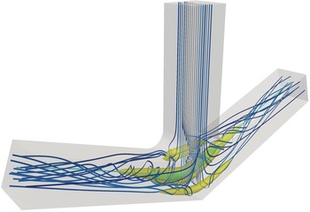
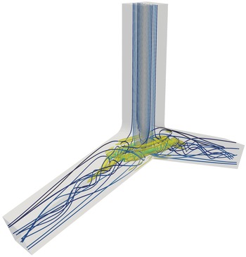
Before we discuss the linear stability and sensitivity results for pipe bifurcations in § 4, it is worth devoting some discussion to the base flow itself. The base flow is described in three sections. First, the geometry is discussed in § 3.1. Next, the T-junction flow is described in § 3.2, and then the arrow- and Y-junction flows are described in § 3.3. We separate the discussion in this way for two reasons. First, we use the T-junction flow as an archetypal example of pipe bifurcation flows, so we describe the vortex behaviour in greater detail for that flow. Second, the T-junction base flow remains symmetric not only across the two outlets, but also between the back and front surfaces (see figure 1). On the other hand, the arrow- and Y-junction flows exhibit supercritical pitchfork bifurcations, which introduce stable front–back asymmetric solutions (see figures 2 and 3), whereas the T-junction does not undergo such a bifurcation.


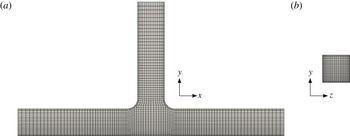
The details of the computational mesh and the mesh validation are discussed in § A.1, and the boundary conditions are covered in § A.2. The algorithms and software are described in § A.3.
3.1 Geometry
The pipe bifurcation geometries we employ have a square cross-section. Figure 1 shows the
 $90^{\circ }$
T-junction used in our computations, along with the associated lengths and axes. The
 $x$
-axis is aligned with the outlet pipes, and
 $x=0$
is the centre plane halfway between the two outlets. The
 $y$
-axis is aligned with the inlet pipe, and
 $y=0$
is the bottom surface. Finally, the
 $z$
-axis is the depth direction, and
 $z=0$
is the plane halfway between the front and back walls of the junction. With a cross-section of
 $1\times 1$
, the inlet pipe measures five units from the inlet to the bottom of the junction, and each outlet pipe measures five units from the outlet to the centre plane between the two outlets. For the Reynolds numbers we consider here, these dimensions are sufficient for approximating a junction with an infinitely long inlet and infinitely long outlets. In one test at
 $Re=560$
, extending the outlets to 10 units caused the leading eigenvalue of
 $\mathscr{L}$
to shift by a distance of
 $6.41\times 10^{-3}$
in the complex plane. In another, shortening the inlet to three units caused the leading eigenvalue of
 $\mathscr{L}$
to shift by
 $1.61\times 10^{-3}$
, and the corresponding eigenvalue of
 $\mathscr{L}^{\ast }$
to shift by
 $1.76\times 10^{-3}$
.
The right-angle corners of the junction are rounded with quarter circles. For our analyses, the radius of curvature at these corners is
 $R=0.4$
to match experiments reported by Vigolo et al. (Reference Vigolo, Radl and Stone2014), unless we state otherwise. The radii of curvature
 $R=0$
, i.e. a square corner, and
 $R=1$
are also explored. We used these radii of curvature in our previous work (Chen et al.
Reference Chen, Rowley and Stone2015).
The
 $\unicode[STIX]{x1D703}=70^{\circ }$
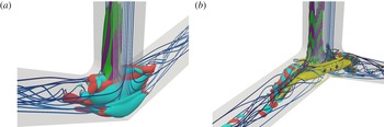
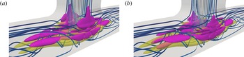
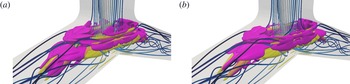
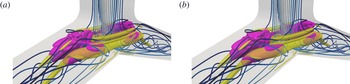
arrow-junction is shown in figure 2 and the
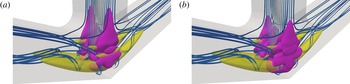
 $\unicode[STIX]{x1D703}=110^{\circ }$
Y-junction in figure 3. The outlet lengths remain at five units long, and the radius of curvature remains at
 $R=0.4$
. These two figures depict the flows near the Hopf bifurcation of the stable asymmetric branch past the supercritical pitchfork bifurcation.
3.2 T-junction
3.2.1 Reynolds number dependence and vortex pair description
Denoting the dimensional average inlet speed by
 $U$
and pipe width by
 $L$
, the Reynolds number is
 $Re=\unicode[STIX]{x1D70C}UL/\unicode[STIX]{x1D707}$
. For each junction corner radius of curvature
 $R$
, we have computed a single continuous branch of steady-state solutions spanning up to
 $10\leqslant Re\leqslant 650$
; see figure 4. With the methodology we presented in § A.3, we are unable to detect any other branches, stable or unstable, in this Reynolds-number range. Nevertheless, given the complexity of the solution branches for the far simpler Dean flow (Winters Reference Winters1987), we posit that there ought to exist additional branches that we have not found. With
 $R=0.4$
, which is the focus of our article, the base flow we compute is a simplification of the bubble-laden T-junction flow reported by Vigolo et al. (Reference Vigolo, Radl and Stone2014). Although our simulations assume a constant-density single-phase flow, the physical phenomena and Reynolds-number regimes have close similarities with the experiments. We also remark that for the range of Reynolds numbers we have studied, both the base flow and the leading direct and adjoint eigenmodes are symmetric about the
 $x=0$
plane (i.e. across the outlet direction) and the
 $z=0$
plane (i.e. across the depth direction). Therefore, in some of the following figures, we will only show part of the domain for brevity.
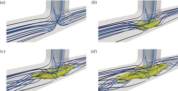
The steady-state solution branch for
 $R=0.4$
, shown as velocity streamlines (blue, low speed; grey, high speed) and a single level set of the
 $Q$
-contour (yellow); cf. figure 1 at
 $Re=560$
: (a)
 $Re=50$
; (b)
 $Re=100$
; (c)
 $Re=200$
; (d)
 $Re=320$
, near the onset of vortex breakdown (see figure 6
b).

A key feature of the T-junction flow is that the impacting of the inlet flow against the junction induces a curvature in the velocity streamlines. Much like the fully developed Dean flow through a slowly bending pipe, the centrifugal force associated with this curvature induces a secondary flow and a large vortex pair in the junction. At sufficiently high Reynolds number, the inertia from the inlet flow creates very strong swirl in the vortex pair. The vortex pair becomes a dominant feature of the flow for approximately
 $Re\geqslant 100$
(figure 4
b). At approximately
 $Re\geqslant 200$
(figure 4
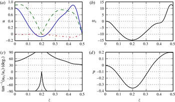
c), the large vortex pair also visibly induces further counter-rotating vortex pairs. Figure 5 shows the velocity components, axial vorticity, swirl and pressure profiles of one such vortex, as a function of the depth dimension
 $z$
, at the higher
 $Re=560$
. A visual inspection of this figure reveals that each vortex in the pair bears some resemblance to the Batchelor vortex (Batchelor Reference Batchelor1964), at least around the vortex core. In the Batchelor vortex, the axial velocity
 $u_{x}$
and azimuthal velocity
 $u_{\unicode[STIX]{x1D703}}$
are Gaussian functions of the radius with some constant offset, the radial velocity
 $u_{r}$
is zero and the axial vorticity
 $\unicode[STIX]{x1D714}_{x}$
is a Gaussian function of the radius.
The profile of an outlet vortex at
 $x=1.5$
and
 $y=0.415$
, for
 $Re=560$
and
 $R=0.4$
. The vortex core is near
 $z=0.2$
. (a) The axial velocity
 $u_{x}$
(blue solid line), azimuthal velocity
 $u_{\unicode[STIX]{x1D703}}$
(green dashed line) and radial velocity
 $u_{r}$
(red dash-dotted line). (b) The axial vorticity
 $\unicode[STIX]{x1D714}_{x}$
. (c) The swirl angle
 $\tan ^{-1}(u_{\unicode[STIX]{x1D703}}/u_{x})$
. (d) The pressure
 $p$
.

3.2.2 Vortex breakdown
As the Reynolds number increases past that of vortex pair formation, the next major feature of interest is the occurrence of vortex breakdown. This vortex breakdown first occurs near
 $Re=315$
, at which the base flow is stable. Vigolo et al. (Reference Vigolo, Radl and Stone2014) previously reported the occurrence at
 $Re=350$
in an experimental bubble-laden flow and a single-phase computation. At
 $Re=320$
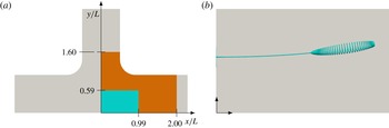
, figure 4(d) depicts the overall flow behaviour, and figure 6(b) specifically shows a streamline on the boundary of the small recirculation region. Below a Reynolds number of approximately 315, the recirculation vanishes. It should be noted that figure 6(b) depicts a traditional bubble-type vortex breakdown, where the approach flow meets an upstream stagnation point that marks the beginning of the recirculation region. In contrast, at higher
 $Re$
(figure 7
a), the recirculation regions are flush against the centre plane
 $x=0$
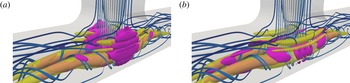
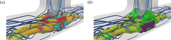
between the two outlets. In this case, the approach flow is from the inlet pipe, and is perpendicular to the recirculation region vortex axis. Ault et al. (Reference Ault, Fani, Chen, Shin, Gallaire and Stone2016) address the transition between these two stages, for which the shift in streamline topology can be described with local bifurcations. In either case, the downstream extent of the recirculation region is a point that we denote the ‘outlet stagnation point’, as in Chen et al. (Reference Chen, Rowley and Stone2015).
(a) The portion of the domain shown in (b) (cyan) and figure 7(a) (orange), with
 $R=0.4$
. (b) Streamlines showing the approach flow and recirculation at the onset of vortex breakdown, at
 $Re=320$
.

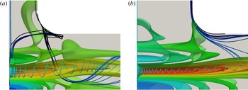
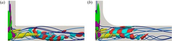
Pressure contours (red, low pressure; green, medium pressure; blue, high pressure), streamlines of the vortical behaviour (cyan) and flow separation streamlines (black, low speed; blue, high speed) past the junction corner, at
 $Re=560$
and
 $R=0.4$
. Only the right half is shown to highlight the effective cross-section. (a) The default geometry, as in figure 1, with vortex breakdown indicated by the recirculating streamline. (b) With an inlet width of
 $2L$
instead of
 $L$
; the vortex breakdown disappears.

As previously mentioned, there has been much debate for many decades about the cause of vortex breakdown. Although we do not speculate about the cause, we do note that the T-junction flow contains all of the hallmark characteristics of a vortex breakdown. In particular, Hall (Reference Hall1972) identified three features common to vortex breakdown. The first is that the vortex must exhibit a very high swirl angle, as defined by
 $\tan ^{-1}(u_{\unicode[STIX]{x1D703}}/u_{x})$
; Hall reported that the swirl angle must minimally be approximately
 $40^{\circ }$
upstream of the breakdown point. In the T-junction flow at
 $Re=320$
, the swirl angle is nearly
 $90^{\circ }$
upstream of the breakdown (not shown). Furthermore, at
 $Re=560$
, the swirl angle is not far from
 $90^{\circ }$
through much of the vortex; see figures 5(c) and 7(a).
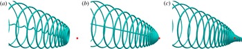
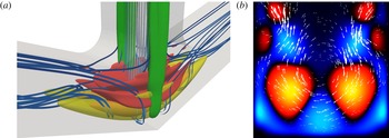
The second feature is that streamlines converge towards or diverge from the vortex core, depending on the orientation relative to the recirculation bubble. Figure 8(a) shows that after a streamline inside the recirculation region begins to reverse direction just upstream of the outlet stagnation point, it spirals towards the vortex core. The same effect occurs in figure 8(c), where a streamline just outside the bubble converges to the vortex core, just downstream of stagnation. The boundary of the recirculation bubble, along with the reverse-flow vortex core, is shown in figure 8(b). The behaviour near the upstream stagnation point of figure 6(b) implies an analogous streamline divergence.


Finally, there must be an adverse pressure gradient in the axial direction, which Vigolo et al. (Reference Vigolo, Radl and Stone2014) reported in T-junction flow, and which we verify in figure 7(a). There are at least three reasons for the adverse pressure gradient in the outlets of the T-junction at these modest Reynolds numbers. First, as the flow navigates from the inlet to the outlets, the cross-section of the pipe effectively doubles from
 $1\times 1$
to
 $2\times 1$
because of the two outlet pipes. The net result is that the average velocity is halved, thereby introducing an adverse pressure gradient. Second, the swirl, as measured by the azimuthal velocity, is very strong where the inlet flow impacts the junction wall. By the radial component of the Navier–Stokes equation, the pressure difference between the vortex core and the vortex exterior must be large. As the flow moves towards the outlets, however, viscous effects in the flow weaken the azimuthal velocity. The pressure difference must weaken as well, indicating that the pressure in the vortex core will increase downstream. Third, there exists a flow separation at the junction corners, which is prominent when
 $R=0$
, albeit less so when
 $R=0.4$
or 1. Even in the latter cases, however, the flow separation takes the form of a vertical vortex pair at each corner, flushing fluid downward between the large outlet vortices. With the presence of the vertical vortex pair, the duct bears some similarity to a converging–diverging nozzle. Figure 7(a) shows that the diverging part of the flow – as the flow navigates past the separation bubble – is in fact connected to a weak addition to the adverse pressure gradient.
We can remove the first contribution to the adverse pressure gradient, the effective doubling of the pipe cross-section, if we make the inlet twice as wide in the
 $x$
direction. Maintaining a cross-section of
 $1\times 1$
in each outlet, we now widen the inlet cross-section to
 $2\times 1$
. We redefine the Reynolds number by
 $Re=\unicode[STIX]{x1D70C}UL_{h}/\unicode[STIX]{x1D707}$
, where
 $U$
is still the dimensional average inlet speed, and
 $L_{h}=4L/3$
is the dimensional hydraulic diameter of the inlet. It should be noted that the use of the hydraulic diameter here does not change the Reynolds number for the default case of a square inlet. Figure 7(b) reveals that at
 $Re=560$
, the adverse pressure gradient actually still remains strong, but the swirl angle decreases. Furthermore, the pressure contours show that the adverse pressure gradient at the junction corner is reduced, and the streamlines show that the flow separation is minimal. In this case, the vortex breakdown disappears at this
 $Re$
, but the reason is not presently clear, and indicates another avenue for future studies.
3.2.3 Hopf bifurcation
Returning to the square inlet cross-section, the next feature of interest past the appearance of vortex breakdown near
 $Re=320$
is the first Hopf bifurcation. Denoting the Reynolds number of the first instability by
 $Re_{H}$
, this Reynolds number is
 $Re_{H}=587$
for
 $R=0$
,
 $Re_{H}=556$
for
 $R=0.4$
and
 $Re_{H}=552$
for
 $R=1$
. Below
 $Re_{H}$
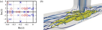
, the base flow is stable, and would be in agreement with single-phase flow experiments or time-resolved simulations that are allowed to run indefinitely. As the Reynolds number increases past the Hopf bifurcation point, however, one pair of eigenvalues crosses from the stable complex left half-plane to the unstable right half-plane. Figure 9(a) shows two such Hopf bifurcations on the same solution branch in quick succession.
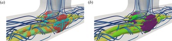
(a) Eigenvalues at
 $Re=500$
(red circles) and 560 (blue crosses) for
 $\unicode[STIX]{x1D703}=90^{\circ }$
and
 $R=0.4$
. (b) Time-resolved snapshot of an unsteady helical oscillation at
 $Re=570$
; cf. figure 1.

At
 $Re>Re_{H}$
, the equilibrium is unstable – though it is still solvable with Newton iteration – and the observed flow in an experiment or time-resolved simulation is a stable oscillating flow. The oscillations take the form of helical, i.e. corkscrew, motions in the outlet vortex pairs that co-rotate with the direction of swirl. As such, the helical mode is symmetric about the vertical plane
 $z=0$
separating the two vortices. The mode is also symmetric about the vertical plane
 $x=0$
between the two outlets. The helical oscillation has an axial wavelength roughly 2.5 times the separation between the two vortices. Figure 9(b) depicts a snapshot of this helical motion. We note that the T-junction instability contrasts with the free vortex pair instabilities of Crow (Reference Crow1970) and Leweke & Williamson (Reference Leweke and Williamson1998). In the former, the instability is manifested on planes inclined
 $48^{\circ }$
from the line joining the vortices, is symmetric and has a wavelength 8.6 times the vortex spacing. In the latter, the instability is antisymmetric and has a wavelength 0.8 times the vortex spacing. The effects of the walls are undoubtedly large in the T-junction.
The Hopf bifurcation appears to be supercritical, based on numerical simulations near the bifurcation point, although the rigorous determination of this criticality is outside the scope of this article. Various methods for rigorously determining the criticality may be employed. The use of a weakly nonlinear analysis may reveal the sign of the cubic nonlinearity in the Landau-type amplitude equation (e.g. Yuen & Bau Reference Yuen and Bau1996; Chomaz Reference Chomaz2005), which corresponds to the criticality of the bifurcation. Centre manifold calculations, as described by Guckenheimer & Holmes (Reference Guckenheimer and Holmes1983, chap. 3), may also be employed. Finally, careful computation of time-resolved solutions in the vicinity of the bifurcation point may reveal the nature and stability of limit cycles (e.g. Mamun & Tuckerman Reference Mamun and Tuckerman1995). The question of Hopf criticality may be further explored in future work.
3.3 Arrow- and Y-junctions
The single-phase, bubble-laden and particle-laden flows through pipe bifurcations with angles ranging from
 $\unicode[STIX]{x1D703}=30^{\circ }$
to
 $120^{\circ }$
are described in Ault et al. (Reference Ault, Fani, Chen, Shin, Gallaire and Stone2016). We refer readers to this work for additional details about flows through arrow- and Y-junctions, such as Reynolds-number effects, qualitative and quantitative descriptions of the vortex breakdown and the capture of bubbles and particles in the recirculation zones.
In a rough sense, the flow behaviour for smaller values of
 $\unicode[STIX]{x1D703}$
intuitively has a natural equivalence with Dean flows with smaller centreline radii of curvature
 $a$
. Given that the Dean flow with pipe diameter
 $d$
is characterised primarily by the Dean number
 $\mathit{Dn}=Re\sqrt{d/(2a)}$
, there is a natural expectation that flow features in curved pipes with smaller
 $a$
will be exhibited at smaller
 $Re$
. The same is essentially true in pipe bifurcation flow, where phenomena such as vortex breakdown and local bifurcations occur at lower
 $Re$
for lower
 $\unicode[STIX]{x1D703}$
. A description of the onset of breakdown at various junction angles can be found in the article by Ault et al. (Reference Ault, Fani, Chen, Shin, Gallaire and Stone2016).
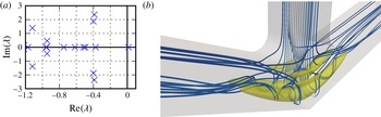
(a) Eigenvalues at
 $Re=170$
for
 $\unicode[STIX]{x1D703}=70^{\circ }$
, near the supercritical pitchfork bifurcation at
 $Re=168$
. (b) The symmetric solution at
 $Re=170$
, which does not contain recirculation; cf. figure 2.

As mentioned above, however, the Dean description is insufficient for pipe bifurcation flow because of the inherent three-dimensionality. In the
 $70^{\circ }$
arrow-junction (figure 2), the recirculation regions are initially aligned orthogonally to the inflow, but quickly turn towards the outlets because of the upward-sloped bottom wall. In contrast, the
 $110^{\circ }$
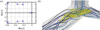
Y-junction (figure 3) allows the vortex core of the recirculation regions to remain essentially orthogonal to the inflow. The counter-rotating vortices form near the bottom of the pipe intersections, and do not encounter the downward-sloping top walls for some distance.
One of the key features that distinguishes arrow- and Y-junction flows from T-junction flow is the supercritical pitchfork bifurcation that renders the stable steady-state solution asymmetric for a certain Reynolds number range. This pitchfork bifurcation occurs at
 $Re=168$
for
 $\unicode[STIX]{x1D703}=70^{\circ }$
(figure 10) and
 $Re=649$
for
 $\unicode[STIX]{x1D703}=110^{\circ }$
(figure 11), and was not reported by Ault et al. (Reference Ault, Fani, Chen, Shin, Gallaire and Stone2016). Figures 2 and 3 show the stable asymmetric solutions at
 $Re=190$
for
 $\unicode[STIX]{x1D703}=70^{\circ }$
and
 $Re=698$
for
 $\unicode[STIX]{x1D703}=110^{\circ }$
respectively. In the former case, recirculation is only present in the rear half of the domain. The establishment of the bifurcation as a supercritical pitchfork type is evident from the appearance of stable asymmetric steady states, as well as the rearrangement of the vortex pair in the direction of the antisymmetric centre eigenmode.
(a) Eigenvalues at
 $Re=650$
for
 $\unicode[STIX]{x1D703}=110^{\circ }$
, near the supercritical pitchfork bifurcation at
 $Re=649$
. (b) The symmetric solution at
 $Re=650$
; cf. figure 3.

The supercritical pitchfork bifurcation in arrow- and Y-junctions is reminiscent of the pitchfork bifurcation in cross-slot flow (Haward et al. Reference Haward, Poole, Alves, Oliveira, Goldenfeld and Shen2016), where two opposing sides of a ‘+’ shape are inlets and the opposing sides in the orthogonal direction are outlets. The nature of that bifurcation is different, however. Instead of exhibiting an asymmetric vortex pair the bifurcation is rather the formation of a single spiral vortex. In the experiments, the orientation of the rotation was determined by geometrical imperfections in the apparatus. Although the cross-slot geometry bears close similarity to the T-junction, the key difference is that the T-junction enforces the no-penetration and no-slip condition in what would be the plane dividing the two inlets of the cross-slot. Therefore, the single spiral vortex cannot form around this plane.
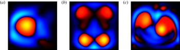
In fact, it is noteworthy that the T-junction does not exhibit any pitchfork bifurcations at Reynolds numbers below that of the first Hopf bifurcation. As figure 9 implies, the stable periodic orbit of the Hopf bifurcation displays symmetry not only between the two outlets, but also between the front and back walls. Figure 12(b) also shows this front–back symmetry, and a weaker vortex pair with rotation opposite to the main vortex pair is visible at the top of the pipe. In contrast, the post-bifurcation asymmetry in the arrow- and Y-junctions (figure 12 a,c) causes the main vortex pair to align diagonally across each outlet pipe. Additionally, the secondary vortex pair is either smaller and weaker, or not present at all. Currently, we do not have a rigorous explanation for the absence of the pitchfork bifurcation in the T-junction; this remains a topic for further study. It is reasonable to suppose that for maximal stability, the preferential arrangement of the vortex pair, whether symmetrically or diagonally, can be explained by the physics of the flow turning through the junction.
Normal slices of an outlet pipe two units of displacement from the junction centre, showing
 $Q$
(red,
 $Q>0$
; blue,
 $Q<0$
; colours exaggerated for clarity): (a)
 $\unicode[STIX]{x1D703}=70^{\circ }$
and
 $Re=190$
(see figure 2); (b)
 $\unicode[STIX]{x1D703}=90^{\circ }$
and
 $Re=560$
(see figure 1); (c)
 $\unicode[STIX]{x1D703}=110^{\circ }$
and
 $Re=698$
(see figure 3).

We also briefly remark that our complementary flow experiments (Ault et al. Reference Ault, Fani, Chen, Shin, Gallaire and Stone2016) show an asymmetry between the two outlets under certain conditions. Our simulations do not reveal any such mechanism, but this may be a limitation of the pressure boundary conditions prescribed at the outlet (see § A.2). To investigate such asymmetries, a less rigid pressure condition would probably be required.
At Reynolds numbers higher than that of the supercritical pitchfork bifurcation, the symmetric branch and both asymmetric branches next undergo Hopf bifurcations. For
 $\unicode[STIX]{x1D703}=70^{\circ }$
, the asymmetric branches are projected to bifurcate at
 $Re=200$
and the symmetric branch at
 $Re=184$
. For
 $\unicode[STIX]{x1D703}=110^{\circ }$
, the asymmetric branches are projected to bifurcate at
 $Re=699$
and the symmetric branch at
 $Re=698$
. Only the bifurcation of the asymmetric branches would be directly observed in an experiment or time-resolved simulation. The nature of the centre eigenmodes is briefly discussed in § 4.2.
4 Eigenmode analysis
4.1 T-junction
A common feature of inertia-dominated convective flows (i.e.
 $Re\gg 1$
) is that direct eigenmodes tend to be large only in a downstream region of the flow, and that adjoint eigenmodes tend to be large only in an upstream region. To list a few examples, Åkervik et al. (Reference Åkervik, Hœpffner, Ehrenstein and Henningson2007), Giannetti & Luchini (Reference Giannetti and Luchini2007), Qadri et al. (Reference Qadri, Mistry and Juniper2013) and Fani et al. (Reference Fani, Camarri and Salvetti2013) report these features respectively for the flow over a shallow cavity, the flow around a cylinder, a swirling jet with vortex breakdown and a mixing T-junction flow. This response is largely because the base flow transports flow perturbations, as described by the second term in the linearised Navier–Stokes operator (2.3). On the other hand, it is the negative of the base flow that transports adjoint flow perturbations, as described by the second term in the adjoint operator (2.6). As a result,
 $Re\gg 1$
flows tend to be strongly non-normal. Direct eigenmodes are typically nearly parallel to each other, as are adjoint eigenmodes; see Schmid & Henningson (Reference Schmid and Henningson2001) for a more complete discussion.
For the large Reynolds numbers of interest here, we observe the same types of non-normal responses in our pipe bifurcation flows. For reference, figure 9(a) shows the eigenvalues of the linearised Navier–Stokes operator with
 $\unicode[STIX]{x1D703}=90^{\circ }$
,
 $R=0.4$
and
 $Re=560$
, near the first Hopf bifurcation at
 $Re=556$
. Figure 13 shows the two least stable direct and adjoint eigenmodes, which correspond to
 $\unicode[STIX]{x1D706}_{1}=0.003\pm 2.208\text{i}$
and
 $\unicode[STIX]{x1D706}_{2}=0.000\pm 1.534\text{i}$
. Since the most unstable eigenmode (figure 13
a) is close to the centre mode of the Hopf bifurcation, this eigenmode is the representation of the helical oscillation that appears after the steady-state base flow loses stability, as described in § 3. The most unstable eigenmode has its largest magnitude in and near the outlet vortex pairs, just downstream of the junction. The axial wavelength of the eigenmode oscillations is approximately two and a half times the spacing between the vortex cores. This feature is in agreement with the axial wavelength of the helical oscillations we observe in the time-resolved flow at
 $Re=570$
, shown in figure 9(b). This direct eigenmode is also large in a smaller weaker vortex pair at the top of the outlet pipes, which is not directly visible in figure 13 but can be seen in figure 12(b). Time-resolved simulations show that the periodic orbit arising from the Hopf bifurcation involves oscillations of all four vortices in the outlet pipes.
Direct and adjoint eigenmodes for the T-junction flow at
 $Re=560$
and
 $R=0.4$
. The direct eigenmodes are shown as single level sets of the pointwise norms
 $\Vert \text{Re}(\unicode[STIX]{x1D753})\Vert$
(red) and
 $\Vert \text{Im}(\unicode[STIX]{x1D753})\Vert$
(cyan); the adjoint eigenmodes are shown as single level sets of
 $\Vert \text{Re}(\unicode[STIX]{x1D74D})\Vert$
(green) and
 $\Vert \text{Im}(\unicode[STIX]{x1D74D})\Vert$
(purple). Streamlines (blue, low speed; grey, high speed) and a
 $Q$
-contour (yellow) are overlaid. (a) The most unstable eigenmode,
 $\unicode[STIX]{x1D706}_{1}=0.003\pm 2.208\text{i}$
. (b) The second least stable eigenmode,
 $\unicode[STIX]{x1D706}_{2}=0.000\pm 1.534\text{i}$
.

Whereas the first eigenmode
 $\unicode[STIX]{x1D753}_{1}$
loses stability at
 $Re=556$
, the next several modes lose stability at only slightly higher
 $Re$
(Chen et al.
Reference Chen, Rowley and Stone2015). The close proximity of their critical Reynolds numbers suggests that the solution branch rapidly becomes complex as
 $Re$
increases. As shown in figure 13(b), the second direct eigenmode
 $\unicode[STIX]{x1D753}_{2}$
is largest in a region that is further downstream than the first eigenmode. We find that the third direct eigenmode is qualitatively very similar to the second; the fourth direct eigenmode is qualitatively very similar to the first; in fact, all further eigenmodes that we investigated resemble the first or second least stable eigenmodes. These results are in line with previous studies at similar Reynolds numbers (e.g. Åkervik et al.
Reference Åkervik, Hœpffner, Ehrenstein and Henningson2007, for the flow over a shallow cavity), which have demonstrated that eigenmodes tend to be nearly parallel, occupying almost the same area in space, with very similar physical structures.
The adjoint eigenmodes
 $\unicode[STIX]{x1D74D}$
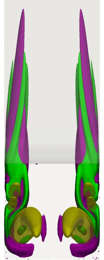
, in contrast, are large only in a small upstream region of the flow. This region, which figure 13 shows for the first and second modes, resides in the inlet and the junction, along the front and back walls. Specifically, the region of large
 $\unicode[STIX]{x1D74D}$
wraps around the counter-rotating vortex pairs in the junction; see figure 14. Typically, the adjoint eigenmodes are larger just outside the vortices than inside. Based on the linear receptivity theory we reviewed in § 2.2, the choice of initial conditions and the placement of external disturbances outside the vortex pairs has a greater effect on the linearised dynamics (2.12) than those inside. In addition, the receptivity region in the inlet pipe bears notable resemblance to adjoint impulse responses and modes that others have computed for the flat plate boundary layer (e.g. Bagheri, Brandt & Henningson Reference Bagheri, Brandt and Henningson2009). In general, the adjoint eigenmodes show even less variation among mode numbers than the direct eigenmodes. The similarity among adjoint eigenmodes hints that the linear receptivity mechanisms in this flow are highly localised only to a small region external to the vortices.
View from an outlet of the most unstable adjoint eigenmode (green and purple) shown in figure 13(a), for
 $\unicode[STIX]{x1D703}=90^{\circ }$
,
 $Re=560$
and
 $R=0.4$
.

Two additional details are worthy of note. First, as mentioned above, the leading eigenmodes are symmetric about the
 $x=0$
and
 $z=0$
planes, which is consistent with the symmetry of the geometry. In fact, at least the first 10 modes are symmetric, and any antisymmetric or asymmetric modes would have eigenvalues far in the complex left half-plane. The symmetry of the leading modes is in contrast to the dynamics in arrow- and Y-junctions, which is discussed in § 4.2. Second, the junction corner radius of curvature does not appear to play a major role in the stability and receptivity characteristics of the flow. Figure 15 shows the least stable direct and adjoint eigenmodes close to the first Hopf bifurcation for
 $R=0$
and 1. As in the default case of
 $R=0.4$
, the direct eigenmodes reside primarily in the outlet pipes, either near the inlet–outlet intersection or further downstream, and the adjoint eigenmodes reside in a small region near the walls of the inlet and junction.
The centre direct (red and cyan) and adjoint (green and purple) eigenmodes close to the first Hopf bifurcation, for different junction corner radii of curvature. Only the right half is shown for brevity: (a)
 $R=0$
and
 $Re=590$
; (b)
 $R=1$
and
 $Re=550$
.

4.2 Arrow- and Y-junctions
For the pipe bifurcations with
 $\unicode[STIX]{x1D703}=70^{\circ }$
and
 $110^{\circ }$
, we briefly comment on the centre eigenmode corresponding to the supercritical pitchfork bifurcations near
 $Re=170$
and
 $650$
respectively. The eigenvalues and symmetric solutions are shown in figures 10 and 11, and the stable asymmetric solutions at slightly higher Reynolds numbers are shown in figures 2 and 3. The centre eigenmodes themselves are shown in figures 16 and 17. In both cases, the centre eigenmode remains symmetric about
 $x=0$
(that is, the plane between the two outlets), but an antisymmetry about
 $z=0$
(that is, between the front and back walls) is present; refer to figure 1 for the coordinate axes. Specifically, the
 $x$
- and
 $y$
-components of
 $\boldsymbol{u}$
are antisymmetric about
 $z=0$
, and the
 $z$
-component is symmetric (figures 16
b and 17
b).
The centre eigenmode for the
 $\unicode[STIX]{x1D703}=70^{\circ }$
pitchfork bifurcation at
 $Re=170$
. (a) Single level sets of the pointwise norms
 $\Vert \unicode[STIX]{x1D753}\Vert$
(red) and
 $\Vert \unicode[STIX]{x1D74D}\Vert$
(green). (b) The slice
 $x=0$
between the two outlets, showing
 $Q$
(red,
 $Q>0$
; blue,
 $Q<0$
) and
 $\unicode[STIX]{x1D753}$
vectors (white) scaled by
 $\Vert \unicode[STIX]{x1D753}\Vert$
.

The centre eigenmode for the
 $\unicode[STIX]{x1D703}=110^{\circ }$
pitchfork bifurcation at
 $Re=650$
. See the caption to figure 16. (b) An orthogonal slice three units downstream of the junction centre, as viewed from the outlet. Vectors into the plane are obscured by the plane to emphasise the out-of-plane component, which is antisymmetric.

For both angled junctions, the primary effect of the asymmetry is the rearrangement of the outlet-oriented vortices in each outlet pipe, as shown in figures 16(b) and 17(b). The two components of the centre eigenmode normal to the streamwise direction are generally larger than the streamwise component. These two dominant components essentially push one of the large vortices downward while pushing the counter-rotating counterpart upward. Such an effect on the smaller counter-rotating vortices is also significant in figure 16(b). The rearrangements caused by the centre eigenmode can be seen in figure 12(a,c).
It is of particular note that in the
 $\unicode[STIX]{x1D703}=70^{\circ }$
junction, the asymmetric branch of the pitchfork bifurcation exhibits recirculation in half of the junction at
 $Re=180$
(figure 2), but no recirculation is observed at the bifurcation point. Ault et al. (Reference Ault, Fani, Chen, Shin, Gallaire and Stone2016) also do not report any recirculation in the symmetric solution at
 $Re=180$
. Therefore, the appearance of the recirculation in the asymmetric branch can be attributed, at least in part, to the antisymmetric centre eigenmode.
The eigenmodes corresponding to the Hopf bifurcation on the stable asymmetric branch: (a)
 $\unicode[STIX]{x1D703}=70^{\circ }$
and
 $Re=190$
(cf. figure 2); the
 $Q$
contour is excluded for clarity; (b)
 $\unicode[STIX]{x1D703}=110^{\circ }$
and
 $Re=698$
(cf. figure 3). See the colour legend in the caption to figure 13.

Another significant difference between the centre eigenmodes at
 $\unicode[STIX]{x1D703}=70^{\circ }$
and
 $110^{\circ }$
is the downstream position. At
 $\unicode[STIX]{x1D703}=70^{\circ }$
(figure 16
a), the eigenmode is largest in the dominant vortex structures in the pipe intersection; at
 $\unicode[STIX]{x1D703}=110^{\circ }$
(figure 17
a), it is largest substantially further downstream. Intuitively, this effect can probably be primarily attributed to the difference in Reynolds number at the pitchfork bifurcations. The arrangement of the centre eigenmode in the downstream direction dictates the asymmetry arising from the pitchfork bifurcation. Figure 2 shows that the asymmetric branch at
 $\unicode[STIX]{x1D703}=70^{\circ }$
is strongly asymmetric in and near the pipe intersection, with recirculation present in only one half of the junction. In contrast, the asymmetric branch at
 $\unicode[STIX]{x1D703}=110^{\circ }$
(figure 3) retains symmetry near the junction centre to a large degree. The vortices are noticeably diagonally arranged only after some distance downstream.
The nature of the adjoint centre eigenmodes (figures 16 a and 17 a) is qualitatively similar to what is seen in the Hopf bifurcation of the T-junction. The primary difference is that the centre eigenmode of the pitchfork bifurcation is real-valued, but the physical arrangement of the adjoint mode in space is largely unchanged. For this reason, we do not comment further on the receptivity of the bifurcating modes in the arrow- and Y-junctions.
We also comment on the centre eigenmodes of the Hopf bifurcations that take place on the stable asymmetric branches. In the arrow-junction (figure 18 a), the centre eigenmode – as in the pitchfork bifurcation (figure 16 a) – remains close to the intersection of the inlet and the outlets. Again, the placement of these vortex oscillations is probably the result of the lower Reynolds number leading to a weaker influence of downstream convection in the stability mechanisms. The centre eigenmode of the Y-junction is shown in figure 18(b), and displays an oscillation of the vortex in a downstream location, as in the T-junction (figure 13). In the arrow- and Y-junctions, however, the oscillations corresponding to the periodic orbit arising from the Hopf bifurcation are asymmetric.
5 Sensitivity to spatially localised feedback and base flow modifications
5.1 T-junction
Recently, we described how the sensitivity to spatially localised feedback is connected to the recirculation arising from vortex breakdown (Chen et al.
Reference Chen, Rowley and Stone2015). To reiterate these results briefly, figure 19(a) shows the region of sensitivity to spatially localised feedback for the most unstable eigenmode at
 $Re=560$
, and figure 19(b) shows the sensitivity for the second eigenmode (see (2.21)). We find that all of the regions of sensitivity to spatially localised feedback are qualitatively similar. For all of the eigenmodes we investigated, the overlap between the direct and adjoint eigenmodes is greatest inside, and immediately around, the recirculation regions and the other counter-rotating vortex structures.
The sensitivity to spatially localised feedback for the most unstable eigenmode at
 $Re=560$
and
 $R=0.4$
, shown as the level sets (magenta) (a)
 $|\text{d}\unicode[STIX]{x1D706}_{1}/\text{d}s|=1.25$
and (b)
 $|\text{d}\unicode[STIX]{x1D706}_{2}/\text{d}s|=2.5$
.

Our previous work only considered the magnitude
 $|\text{d}\unicode[STIX]{x1D706}/\text{d}s|$
of this sensitivity. We now extend this analysis by considering in greater detail the effect that feedback has on the stability and frequency of the linearised dynamics. As discussed in § 2.3, the real and imaginary parts of
 $\text{d}\unicode[STIX]{x1D706}/\text{d}s$
describe these effects. Figure 20(a) shows level sets of
 $\text{Re}(\text{d}\unicode[STIX]{x1D706}_{1}/\text{d}s)$
, which dictate the regions where collocated proportional feedback, in the same direction or opposite direction to the flow perturbation from the base flow, would have a stabilising or destabilising effect on the flow. An important implication is that negative feedback is stabilising in most areas inside and around the junction vortices. This result is especially the case inside the recirculation regions arising from vortex breakdown. There, the control strategy of infinitesimally forcing against velocity perturbations is particularly effective at dampening the perturbations. Only within small regions around and inside the vortices, by the intersection of the inlet and outlets, would negative feedback actually destabilise the flow. The discussion of the stabilising or destabilising effect of proportional feedback control is a standard topic in classical control theory and can be understood with Nyquist and root-locus plots (see, e.g., Franklin, Powell & Emami-Naeini Reference Franklin, Powell and Emami-Naeini2010).
(a) Decomposition of the sensitivity to spatially localised feedback (figure 19
a) into regions where negative feedback is stabilising (
 $\text{Re}(\text{d}\unicode[STIX]{x1D706}_{1}/\text{d}s)=1.2$
; red) and destabilising (
 $\text{Re}(\text{d}\unicode[STIX]{x1D706}_{1}/\text{d}s)=-1.2$
; cyan). (b) Decomposition of the sensitivity to spatially localised feedback into regions where negative feedback decreases the oscillation rate (
 $\text{Im}(\text{d}\unicode[STIX]{x1D706}_{1}/\text{d}s)=0.6$
; green) and increases the oscillation rate (
 $\text{Im}(\text{d}\unicode[STIX]{x1D706}_{1}/\text{d}s)=-0.6$
; purple).

Next, we examine the effect of feedback control on the oscillation rate associated with the most unstable eigenmode. Figure 20(b) shows level sets of
 $\text{Im}(\text{d}\unicode[STIX]{x1D706}_{1}/\text{d}s)$
, which dictate the regions where feedback increases or decreases the oscillation rate of the given eigenmode. Since we have arbitrarily chosen to analyse the eigenvalue
 $\unicode[STIX]{x1D706}_{1}=0.003+2.208\text{i}$
instead of its complex conjugate, negative feedback decreases oscillation rates where
 $\text{Im}(\text{d}\unicode[STIX]{x1D706}_{1}/\text{d}s)>0$
, and increases oscillation rates where
 $\text{Im}(\text{d}\unicode[STIX]{x1D706}_{1}/\text{d}s)<0$
. We observe that the application of negative feedback control to velocity perturbations in the smaller vortex pairs above the main pair would decrease the frequency of the mode. The general relation between the location of negative feedback and the associated change in frequency, however, is not immediately clear. The
 $\text{Im}(\text{d}\unicode[STIX]{x1D706}_{1}/\text{d}s)$
field oscillates spatially in multiple directions. Figure 20 does reveal, however, that the regions of growth rate sensitivity and frequency sensitivity essentially coincide.
The sensitivity of the linearised dynamics to base flow modifications is a similar principle to the sensitivity to spatially localised feedback. In both cases, we introduce a perturbation to the linearised operator that we model in a pointwise sense, and we observe the effect of the eigenvalues of the linearisation. Therefore, it is perhaps unsurprising that the sensitivity of the T-junction to base flow modification bears a close resemblance to the sensitivity to spatially localised feedback. Figure 21 shows the sensitivity to base flow modifications with a level set of the pointwise norm
 $\Vert \text{d}\unicode[STIX]{x1D706}/\text{d}\boldsymbol{u}_{0}\Vert$
(see (2.28)); one can note the resemblance to figure 19. Much like the case of spatially localised feedback, the modification of the base flow in and near the vortex structures produces the largest effect on the eigenvalues of the linearisation.
The sensitivity to base flow modifications for the most unstable eigenmodes at
 $Re=560$
and
 $R=0.4$
, shown as the level sets (magenta) (a)
 $\Vert \text{d}\unicode[STIX]{x1D706}_{1}/\text{d}\boldsymbol{u}_{0}\Vert =35$
and (b)
 $\Vert \text{d}\unicode[STIX]{x1D706}_{2}/\text{d}\boldsymbol{u}_{0}\Vert =60$
.

The close relation between the two types of sensitivity is similar in spirit to the cylinder wake analysis reported by Marquet et al. (Reference Marquet, Sipp and Jacquin2008). In Marquet et al.’s analysis, however, the sensitivity to base flow modifications is largest inside the recirculation region, whereas the sensitivity to spatially localised feedback is largest in a more downstream region that includes both the edge of the recirculation as well as the passing free stream. We do not observe this distinction in the T-junction flow.
We may now split the base flow sensitivity into real and imaginary components to analyse the effects of base flow modification on growth rates and frequencies. Figure 22(a) shows level sets of
 $\Vert \text{Re}(\text{d}\unicode[STIX]{x1D706}_{1}/\text{d}\boldsymbol{u}_{0})\Vert$
and
 $\Vert \text{Im}(\text{d}\unicode[STIX]{x1D706}_{1}/\text{d}\boldsymbol{u}_{0})\Vert$
, which spatially oscillate with a small wavelength compared with the vortex spacing and the pipe width. The actual vector directions of
 $\text{Re}(\text{d}\unicode[STIX]{x1D706}/\text{d}\boldsymbol{u}_{0})$
and
 $\text{Im}(\text{d}\unicode[STIX]{x1D706}/\text{d}\boldsymbol{u}_{0})$
, however, are highly complex. Although Marquet et al. (Reference Marquet, Sipp and Jacquin2008) were able to describe the exact base flow modification that had the greatest effect on the eigenvalue growth rate or frequency, we are unable to provide a general description for the T-junction flow.
(a) Decomposition of the sensitivity to base flow modifications (figure 21
a) into the level sets
 $\Vert \text{Re}(\text{d}\unicode[STIX]{x1D706}_{1}/\text{d}\boldsymbol{u}_{0})\Vert =35$
(where base flow modifications change the growth rate; red) and
 $\Vert \text{Im}(\text{d}\unicode[STIX]{x1D706}_{1}/\text{d}\boldsymbol{u}_{0})\Vert =35$
(where base flow modifications change the frequency; cyan). (b) Decomposition of the sensitivity to base flow modifications into the level sets
 $\Vert (\text{d}\unicode[STIX]{x1D706}_{1}/\text{d}\boldsymbol{u}_{0})_{\text{p}}\Vert =35$
(the contribution from production; green) and
 $\Vert (\text{d}\unicode[STIX]{x1D706}_{1}/\text{d}\boldsymbol{u}_{0})_{\text{t}}\Vert =35$
(the contribution from transport; purple); see (2.29).

Following the discussion in § 2.3, we can also decompose the base flow sensitivity into a different set of parts: the contributions from the production and transport of flow perturbations by the base flow modification. Figure 22(b) shows level sets of
 $\Vert (\text{d}\unicode[STIX]{x1D706}_{1}/\text{d}\boldsymbol{u}_{0})_{\text{p}}\Vert$
and
 $\Vert (\text{d}\unicode[STIX]{x1D706}_{1}/\text{d}\boldsymbol{u}_{0})_{\text{t}}\Vert$
to make this distinction. Conceptually, the production and transport terms can be respectively related to local absolute and convective instability (Marquet et al.
Reference Marquet, Sipp and Jacquin2008). The contribution from production dominates in the main vortex pair close to the outlet stagnation point, whereas the contribution from transport is larger near the plane between two outlets. The distinction between the regions of large production and the regions of large transport, however, is not large. Both mechanisms are important where there is large swirl in the base flow. This observation is in contrast to the cylinder wake analysis of Marquet et al. (Reference Marquet, Sipp and Jacquin2008), who observed that the contribution from production dominated the contribution from transport nearly everywhere in the flow.
We remark that at
 $Re=320$
, near the onset of vortex breakdown, the sensitivities to localised feedback and base flow modifications remain strongest near the large vortical structures of the junction; see figure 23. Thus, even when recirculation is very weak or non-existent, perturbations in the linearised dynamics of the horizontal vortices still play a critical role in the location of the linearisation eigenvalues. The connection between the vortices and the sensitivities, however, is not as clear-cut as at higher Reynolds numbers where the recirculation is strong (e.g. figures 19 and 21).
The sensitivities (magenta) of the most unstable mode at
 $Re=320$
and
 $R=0.4$
, at the onset of vortex breakdown. (a) The sensitivity to localised feedback, shown as the level set
 $|\text{d}\unicode[STIX]{x1D706}_{1}/\text{d}s|=2$
. (b) The sensitivity to base flow modifications, shown as the level set
 $\Vert \text{d}\unicode[STIX]{x1D706}_{1}/\text{d}\boldsymbol{u}_{0}\Vert =45$
.

The sensitivity (a) to spatially localised feedback and (b) to base flow modifications for the pitchfork centre eigenmode at
 $\unicode[STIX]{x1D703}=70^{\circ }$
and
 $Re=170$
, shown as the level sets (magenta) (a)
 $\text{d}\unicode[STIX]{x1D706}/\text{d}s=1$
and (b)
 $\Vert \text{d}\unicode[STIX]{x1D706}/\text{d}\boldsymbol{u}\Vert =10$
.

In § 4, we commented on the lack of a notable effect from the junction corner radius of curvature on the direct and adjoint eigenmodes. In our previous work (Chen et al. Reference Chen, Rowley and Stone2015), we also described the same lack of an effect on the sensitivity to spatially localised feedback. We find that the flow separation at the junction corners does not exhibit any particular connection with stability, receptivity, or either type of sensitivity that we have considered. Therefore, the flow separation at the corners does not interact significantly with factors that modify the dynamics or otherwise introduce disturbances. It is presently unclear why the large horizontally oriented vortices produced by the inlet flow are closely connected to the stability and sensitivity of the flow, but the small vertically oriented vortices produced by the flow separation at the corners are not. A possible explanation is that the horizontal vortices exhibit tightly spiralling streamlines, with recirculation appearing at sufficiently high Reynolds numbers; on the other hand, the vortices at the corners do not exhibit as much swirl, and no recirculation is present. This question remains a topic for future study.
5.2 Arrow- and Y-junctions
Next, we describe the sensitivity of the flow in the
 $\unicode[STIX]{x1D703}=70^{\circ }$
and
 $110^{\circ }$
junctions. We focus the discussion on the sensitivities corresponding to the supercritical pitchfork bifurcation. Therefore, the sensitivity can be interpreted as regions where passive or feedback flow control can best stabilise the symmetric solution, or, alternatively, destabilise it and trigger the onset of the asymmetric branch.
The sensitivities to spatially localised feedback and base flow modification are shown in figure 24 for
 $\unicode[STIX]{x1D703}=70^{\circ }$
and
 $Re=170$
, near the supercritical pitchfork bifurcation. We observe that the base flow does not exhibit recirculation at this Reynolds number and junction angle, which is in agreement with Ault et al. (Reference Ault, Fani, Chen, Shin, Gallaire and Stone2016). The sensitivity regions for this flow are only weakly correlated with the outlet-oriented vortices. Similarly to the discussion of the eigenmodes in the arrow-junction flow, this placement of the sensitivity region can probably be attributed to the lower Reynolds number. With a greater effect of viscosity, the swirl is probably not significant enough to exhibit a strong effect of feedback forcing or base flow modification on the stability. Rather, modifications to the linearised Navier–Stokes operator in the counter-rotating vortices may only have a notable influence on the downstream flow, since the streamlines would not be expected to feed the effects of the modifications back upstream. A greater upstream sensitivity can be seen in figure 24 than in the T-junction flow at
 $Re=560$
(figures 19 and 21), where the recirculation effects dominate the sensitivity.
Following the asymmetric branch of the pitchfork bifurcation, the sensitivity of the Hopf mode at
 $Re=190$
shows a different picture. In figure 25, it can be seen that the asymmetry has a significant effect on the sensitivity. Most notably, the sensitivity is much larger on the side of the junction containing the vortex breakdown (see figure 2). In addition, a greater sensitivity can be seen in the recirculation region than in the equivalent position at the pitchfork bifurcation (figure 24), where recirculation is not present. This observation further supports the idea that recirculation can lead to high eigenvalue sensitivity.
The sensitivity (a) to spatially localised feedback and (b) to base flow modifications for the Hopf centre eigenmode on the asymmetric branch at
 $\unicode[STIX]{x1D703}=70^{\circ }$
and
 $Re=190$
, shown as the level sets (magenta) (a)
 $\text{d}\unicode[STIX]{x1D706}/\text{d}s=0.5$
and (b)
 $\Vert \text{d}\unicode[STIX]{x1D706}/\text{d}\boldsymbol{u}\Vert =8$
. Compare with figure 2.

The sensitivity (a) to spatially localised feedback, showing
 $\text{d}\unicode[STIX]{x1D706}/\text{d}s=1.5$
, and (b) to base flow modifications, showing
 $\Vert \text{d}\unicode[STIX]{x1D706}/\text{d}\boldsymbol{u}\Vert =40$
, for the pitchfork centre eigenmode at
 $\unicode[STIX]{x1D703}=110^{\circ }$
and
 $Re=650$
.

Figure 26 shows the sensitivity regions for
 $\unicode[STIX]{x1D703}=110^{\circ }$
at
 $Re=650$
, again near the supercritical pitchfork bifurcation. A notable difference between these sensitivity regions and those of the T-junction (see figures 19 and 21) is that the former include regions on the
 $z=0$
plane between the front and back walls. The inclusion of this region can be partially attributed to the antisymmetry of the bifurcating mode. It is clear from figure 17(b) that the
 $z$
-component of the Y-junction centre eigenmode is large on the
 $z=0$
plane, since the pitchfork bifurcation introduces solutions that are asymmetric across this plane. In contrast, the centre eigenmode of the T-junction Hopf bifurcation (figure 13
a) is fully symmetric across
 $z=0$
, and the
 $z$
-component of the eigenmode is zero on this plane. The function of this centre eigenmode, in light of the Hopf bifurcation, is to cause vortices on either side of
 $z=0$
to undergo symmetric corkscrew oscillations, as shown in figure 9(b). It should not be surprising from (2.21) and (2.28) that to stabilise or destabilise the symmetry about
 $z=0$
in the Y-junction, it is effective to implement feedback or a base flow modification on that plane. On the other hand, to trigger or delay the transition from symmetric base flow to the symmetric periodic orbit in the T-junction, it is not as effective to modify the linearised operator on that symmetry plane.
We also note that the sensitivities of the Y-junction pitchfork bifurcation are not as connected to the recirculation regions as the T-junction Hopf bifurcation. This may be because the Y-junction pitchfork bifurcation primarily induces asymmetry downstream of the recirculation region, whereas the T-junction Hopf bifurcation primarily induces oscillatory motion in the recirculation regions themselves.
Finally, we also very briefly examine the Hopf bifurcation of the asymmetric branch of the Y-junction. In figure 27, the sensitivity clearly shows an asymmetry between the front and back walls of the junction, which is reflective of the arrangement of the vortices in the junction. Furthermore, the bulk of the sensitivity is further downstream from the intersection, as with the pitchfork bifurcation (figure 26).
The sensitivity (a) to spatially localised feedback, showing
 $|\text{d}\unicode[STIX]{x1D706}/\text{d}s|=1$
, and (b) to base flow modifications, showing
 $\Vert \text{d}\unicode[STIX]{x1D706}/\text{d}\boldsymbol{u}\Vert =35$
, for the eigenmode corresponding to the Hopf bifurcation on the asymmetric branch, at
 $\unicode[STIX]{x1D703}=110^{\circ }$
and
 $Re=698$
. Compare with figure 3.

6 Conclusion
We have analysed the constant-density laminar flow through pipe bifurcations, with a focus on the stability and sensitivity analyses of the flow. We first considered T-junctions with a junction corner radius of curvature
 $R=0.4$
. An analysis of the stable steady-state flow reveals complexities that arise with increasing
 $Re$
, as defined by the average inlet flow speed and the pipe width. At approximately
 $Re>100$
, a large counter-rotating vortex pair is noticeable in the junction and outlet pipes because of the momentum from the inlet. When
 $Re$
increases to approximately 200 and beyond, the vortex pair is well defined and induces multiple smaller weaker vortex pairs closer to the inlet.
Near-axisymmetric bubble-type vortex breakdowns appear at four locations in the T-junction when
 $Re\approx 315$
. These breakdowns give rise to recirculation bubbles that exhibit large swirl, a streamline convergence to or divergence from the vortex core near stagnation points and an adverse pressure gradient in the vortex core. The adverse pressure gradient is the result of a number of factors, including the varying effective pipe cross-sectional area, the viscosity-induced downstream decrease in swirl and flow separation at the junction corners. Next, the first Hopf bifurcation occurs at
 $Re=556$
, at which point the steady-state solution becomes unstable. The stable solution we observe is a helical oscillation of the outlet vortex pair, in which the vortex structures corkscrew with the same rotational orientation as the vortices themselves.
We also analysed arrow-junction flow with junction angle
 $\unicode[STIX]{x1D703}=70^{\circ }$
, as well as Y-junction flow with
 $\unicode[STIX]{x1D703}=110^{\circ }$
. Unlike T-junction flow, both of these flows exhibit supercritical pitchfork bifurcations introducing equilibria that are asymmetric between the front and back walls. These pitchfork bifurcations occur at
 $Re=168$
and 649 respectively, and the stable asymmetric branches undergo Hopf bifurcations at
 $Re=200$
and 699. It is presently unknown at which junction angles the pitchfork bifurcation appears, although this question may be investigated parametrically in future work. In the stable asymmetric branches of the arrow- and Y-junctions, the vortex pair is arranged diagonally in the outlet pipes. Specifically, in the arrow-junction, one vortex in the pair is much stronger than the other, and only this stronger vortex exhibits breakdown leading to recirculation.
We focused the stability, receptivity and sensitivity analysis on Reynolds numbers near the T-junction Hopf bifurcation and the arrow- and Y-junction pitchfork and Hopf bifurcations. The direct centre eigenmodes describe the asymmetric solutions arising from the pitchfork bifurcations and the periodic orbits arising from the Hopf bifurcations. They reside primarily in the outlet pipes, either upstream near the intersection with the inlet, or further downstream. The adjoint eigenmodes, which indicate receptivity, are large only in a small region in the inlet and the junction, along the front and back walls. The direct eigenmodes and, in particular, the adjoint eigenmodes have little variation with mode numbers. The similarity among these modes indicates that the stability and receptivity mechanisms are highly localised in this non-normal flow.
The sensitivity of the linearised dynamics to spatially localised feedback is generally largest in the recirculation regions arising from vortex breakdown, as well as in the smaller counter-rotating vortices induced by the main vortex pair. At lower Reynolds numbers, where the recirculation is weak or non-existent, the sensitivity is still greatest near these vortical structures. By specifically analysing the real and imaginary parts of the sensitivity, we located the regions of the domain where collocated proportional negative feedback would most influence the growth rate or frequency of each eigenmode. For example, negative feedback against velocity perturbations is stabilising in much of the vortical structures, but there do exist small regions where negative feedback is actually destabilising.
The sensitivity to base flow modifications resides in a region that is nearly identical to that of the sensitivity to spatially localised feedback. We also showed the real and imaginary parts of this sensitivity, identifying the regions where base flow modifications affect the growth rate and frequency of the eigenmode. In addition, we located the regions where the base flow sensitivity is caused by the production and transport of velocity perturbations by base flow modifications. The production and transport are of the same order of magnitude in the T-junction vortical structures, with stronger production near the outlet stagnation points and stronger transport near the junction centre.
In general, the radius of curvature of the junction corners does not appear to play a major role in the stability and sensitivity analyses of the T-junction flow. We posit that the arrow- and Y-junctions would exhibit similar behaviour, but such a topic can be pursued more rigorously in future research. Furthermore, the sensitivity regions corresponding to pitchfork bifurcations are not as closely correlated with regions of recirculation and high swirl as those corresponding to Hopf bifurcations.
In a sense, the simplicity of pipe bifurcations belies the complexity of the laminar flows they create. It is our hope that these studies will not only deepen our fundamental understanding of flows through split ducts, but also ultimately increase our appreciation and knowledge of flows through arteries and other real-life systems.
Acknowledgements
K.K.C. was funded by the National Science Foundation through the Graduate Research Fellowship Program. Additional support was provided by the Viterbi Postdoctoral Fellowship from the University of Southern California’s Viterbi School of Engineering, as well as the Institute for Defense Analyses, Center for Communications Research – La Jolla. S. Radl and D. Vigolo aided with our understanding of the flow physics. Furthermore, we thank J. Ault for helpful conversations about the flow through pipe bifurcations of various angles. M. Rossi and F. Gallaire provided insight into vortex instabilities, and C. Pantano-Rubino, V. Gururajan and J. Jayachandran assisted with the numerical treatment of boundary conditions. We performed the computations on computational resources supported by the Princeton Institute for Computational Science and Engineering (PICSciE) and the Office of Information Technology’s High Performance Computing Center at Princeton University. We produced the flow visualisations using ParaView and the two-dimensional plots using matplotlib.
Appendix A. Computational set-up
A.1 Mesh
Our computational meshes comprise several sections. Figure 28 depicts the mesh for the default T-junction geometry with the junction corner radius of curvature
 $R=0.4$
. Three of these sections are the inlet and the two outlet pipes past the rounded corners. In these sections, each finite volume cell is long and skinny in the primary direction of the flow. The cells are more elongated closer to the inlet and outlets, where gradients in the flow direction are smaller. In the inlet pipe, the cells are slightly finer in the transverse (
 $x$
) direction closer to the walls. In the outlet pipes, the cells are finer in the transverse (
 $y$
) direction away from the inlet channel. We choose such a cell spacing in the outlet pipes because the vortical flow has larger
 $y$
-derivatives at the bottom of these pipes than at the top.
The finite volume mesh for the default case of
 $R=0.4$
. For clarity, the mesh shown is five times coarser in each of the three directions than the actual mesh. (a) The
 $x$
–
 $y$
(outlet–inlet) plane. (b) The
 $y$
–
 $z$
(cross-section) plane in an outlet pipe.

With the exception of the geometry with square corners (
 $R=0$
), each mesh also has three sections where the inlet pipe expands into the intersection, and where the intersection contracts into the outlet pipes. These sections have an even cell spacing in the primary flow direction. Finally, at the intersection itself, the cells are slightly finer in the
 $x$
direction towards the outlet pipes; gradients tend to be larger where the flow exits the intersection than at the intersection itself.
In the entire geometry, the cells are finer in the depth (
 $z$
) direction closer to the walls. In addition, all cells that touch the walls of the pipe are further cut parallel to the wall, so as to capture boundary layer effects more accurately. For the stability and sensitivity computations, the T-junction mesh has 5 459 520 cells when
 $R=0$
, 6 096 840 cells when
 $R=0.4$
and 7 435 776 cells when
 $R=1$
. With these mesh resolutions, the flow descriptions we provide in this article are sufficiently accurate. For the case where
 $Re=560$
and
 $R=0.4$
, increasing the resolution to 12 082 728 cells shifts the leading eigenvalue by
 $2.42\times 10^{-2}$
, and decreasing the resolution to 3 143 056 cells shifts the leading eigenvalue by
 $3.93\times 10^{-2}$
. Although finer grids could undoubtedly increase the quantitative accuracy of the eigenvalues, the qualitative nature of the flow and its stability is unaffected by further grid refinement.
Nevertheless, for T-junction base flow simulations where we desired particularly high accuracy in the vortex breakdown streamlines (i.e. figures 1, 5, 6(b), 7(a) and 8), we employed grids that were refined in and around the recirculation regions. For
 $Re=320$
(figure 6
b), the grid was refined by a factor of two in each spatial dimension in boxes that extended approximately
 $0.05L$
beyond each recirculation region. The refinement increased the number of finite volume cells from 6 096 840 to 6 807 592. In the case of
 $Re=560$
, which is a larger focus in this article, the grid was also refined by a factor of two in each spatial dimension, this time in a box that extended approximately
 $0.15L$
beyond the recirculation regions. The refinement increased the number of cells to 13 291 412. These mesh refinements caused virtually no quantitative changes in the base flow, let alone any qualitative changes. Thus, we have all but confirmed that the meshes with roughly six million cells are sufficiently refined for the base flow, stability and sensitivity analyses.
The
 $90^{\circ }$
T-junction mesh with the wider inlet (figure 7
b) is constructed the same way, and has 7 164 116 finite volume cells. The meshes for the
 $70^{\circ }$
arrow-junction and the
 $110^{\circ }$
Y-junction are also constructed essentially identically. In both cases, non-rectangular cells are used to transition from the vertical inlet pipe to the angled outlet pipes. The outlet cells are then angled so as to be aligned with the outlet pipes. These two meshes have a radius of curvature
 $R=0.4$
at the corners, and have 5 878 132 and 5 949 980 cells respectively. Because the
 $90^{\circ }$
T-junction mesh with the square inlet was shown to produce more than sufficiently resolved results, further validation was not performed on these meshes.
A.2 Boundary conditions
The boundary conditions for the Navier–Stokes operator
 $\mathscr{N}$
(2.1) are as follows. We set the inlet velocity
 $\boldsymbol{u}$
to the fully developed profile for channels with square cross-sections, which is given by an infinite sum (see White Reference White2005, chap. 3–3.3) that we truncate to 200 terms, since the resulting truncation error is trivially small. At the walls of the junction, we set the no-slip condition
 $\boldsymbol{u}=\mathbf{0}$
. At the outlets, we assume the flow is fully developed; thus,
 $\boldsymbol{n}\boldsymbol{\cdot }\unicode[STIX]{x1D735}\boldsymbol{u}=\mathbf{0}$
. To achieve numerical consistency with the momentum equation, Neumann conditions for pressure are derived for the inlet and walls by taking the dot product of (2.2) with
 $\boldsymbol{n}$
(Gresho & Sani Reference Gresho and Sani1987). Our experience, however, is that the nonlinear operator is more numerically stable when we employ the Dirichlet condition
 $p=0$
at the outlets.
For the linearised Navier–Stokes operator
 $\mathscr{L}$
(2.3), the boundary conditions are determined by the fact that the perturbed fields
 $\boldsymbol{u}_{0}+\boldsymbol{u}^{\prime }$
and
 $p_{0}$
+
 $p^{\prime }$
must satisfy the same aforementioned conditions on
 $\mathscr{N}$
as the equilibrium fields
 $\boldsymbol{u}_{0}$
and
 $p_{0}$
. Thus, at the inlet and walls, we require
 $\boldsymbol{u}^{\prime }=\mathbf{0}$
and we derive Neumann conditions for
 $p^{\prime }$
by taking the dot product of (2.4) with
 $\boldsymbol{n}$
. At the outlets,
 $\boldsymbol{n}\boldsymbol{\cdot }\unicode[STIX]{x1D735}\boldsymbol{u}^{\prime }=\mathbf{0}$
and
 $p^{\prime }=0$
.
Finally, (2.8) is the general boundary condition for the adjoint linearised Navier–Stokes operator
 $\mathscr{L}^{\ast }$
(2.6). Based on the conditions we have already set for
 $\mathscr{N}$
and
 $\mathscr{L}$
, it is sufficient to set
 $-p^{\prime }\bar{\hat{\boldsymbol{u}}}\boldsymbol{\cdot }\boldsymbol{n}+Re^{-1}(\boldsymbol{n}\boldsymbol{\cdot }\unicode[STIX]{x1D735}\boldsymbol{u}^{\prime })\boldsymbol{\cdot }\bar{\hat{\boldsymbol{u}}}=0$
at the inlet and the walls, and
 $-(\boldsymbol{u}^{\prime }\boldsymbol{\cdot }\bar{\hat{\boldsymbol{u}}})(\boldsymbol{u}_{0}\boldsymbol{\cdot }\boldsymbol{n})+\bar{\hat{p}}^{\prime }\boldsymbol{u}^{\prime }\boldsymbol{\cdot }\boldsymbol{n}-Re^{-1}(\boldsymbol{n}\boldsymbol{\cdot }\unicode[STIX]{x1D735}\bar{\hat{\boldsymbol{u}}})\boldsymbol{\cdot }\boldsymbol{u}^{\prime }=0$
at the outlets. Therefore, we enforce
 $\hat{\boldsymbol{u}}=\mathbf{0}$
at the inlet and walls, where, once again, Neumann conditions on pressure are derived from the dot product of (2.11) with
 $\boldsymbol{n}$
. At the outlets, we enforce the Robin condition
 $(\boldsymbol{u}_{0}\boldsymbol{\cdot }\boldsymbol{n})\hat{\boldsymbol{u}}+Re^{-1}\boldsymbol{n}\boldsymbol{\cdot }\unicode[STIX]{x1D735}\hat{\boldsymbol{u}}=\mathbf{0}$
, as well as
 $\hat{p}=0$
.
We make two remarks regarding the boundary conditions. First, at the outlets, the leading adjoint eigenmodes have a pointwise magnitude roughly between
 $10^{-8}$
and
 $5\times 10^{-4}$
. This result is advantageous in the sense that the boundary condition (2.26) of the sensitivity to base flow modifications is automatically approximately satisfied on the entire boundary of our domain. Therefore, as long as
 $\unicode[STIX]{x1D6FF}\boldsymbol{u}_{0}$
is not too large at the outlets, (2.28) yields the sensitivity of the eigenvalues to base flow modifications, to good approximation. We do not need to assume that
 $\unicode[STIX]{x1D6FF}\boldsymbol{u}_{0}=\mathbf{0}$
on the boundary, as is common in the literature (Marquet et al.
Reference Marquet, Sipp and Jacquin2008). Second, in our previous article (Chen et al.
Reference Chen, Rowley and Stone2015), we used the pressure condition
 $\boldsymbol{n}\boldsymbol{\cdot }\unicode[STIX]{x1D735}p=0$
at the inlet and walls. The more consistent pressure conditions (Gresho & Sani Reference Gresho and Sani1987) used in this article produced nearly identical results.
A.3 Algorithms and software
Given a Reynolds number
 $Re$
, we first solve for a steady-state solution
 $\boldsymbol{u}_{0}$
satisfying
 $\mathscr{N}(\boldsymbol{u}_{0})=\mathbf{0}$
. For this task, we employ a Newton iteration with the Armijo rule (Armijo Reference Armijo1966; see also Kelley Reference Kelley1995) to solve for a root of
 $\mathscr{N}$
over the vector field of spatially discretised velocity fields
 $\boldsymbol{u}$
. For this discussion, we will assume that there are
 $n$
finite volume cells in our domain, the spatially discretised velocity field is
 $\boldsymbol{u}\in \mathbb{R}^{3n}$
and
 $\mathscr{N}:\mathbb{R}^{3n}\rightarrow \mathbb{R}^{3n}$
.
We first provide an initial guess
 $\boldsymbol{u}_{1}$
for the true root
 $\boldsymbol{u}_{0}$
. For stable base flows, we can determine this guess by running a time-resolved computational flow solver to long times. Alternatively, to compute steady-state solutions over a range of Reynolds numbers, we use zeroth- or first-order extrapolation from solutions at other Reynolds numbers. Having computed the initial guess, the
 $j$
th iterate of the Newton iteration requires the solution of the Jacobian–vector equation
 $$\begin{eqnarray}\displaystyle \left.\frac{\text{d}\mathscr{N}}{\text{d}\boldsymbol{u}}\right|_{\boldsymbol{u}_{j}}\boldsymbol{h}_{j}=-\mathscr{N}(\boldsymbol{u}_{j}) & & \displaystyle\end{eqnarray}$$
for the Newton step
 $\boldsymbol{h}_{j}\in \mathbb{R}^{3n}$
.
Since
 $n$
is typically very large, we use the generalised minimal residual method (GMRES; Saad & Schultz Reference Saad and Schultz1986; see also Trefethen & Bau III Reference Trefethen and Bau1997, lecture 35, and Kelley Reference Kelley1995, chap. 3) in an inner iteration to solve (A 1) for
 $\boldsymbol{h}_{j}$
. The GMRES method is advantageous for high-dimensional linear systems such as (A 1) because it only requires matrix–vector products. We use a ‘time-stepping’ method (Tuckerman & Barkley Reference Tuckerman and Barkley2000), where we employ the finite difference
 $$\begin{eqnarray}\displaystyle \left.\frac{\text{d}\mathscr{N}}{\text{d}\boldsymbol{u}}\right|_{\boldsymbol{u}_{j}}\boldsymbol{h}_{j}=\frac{\mathscr{N}(\boldsymbol{u}_{j}+\unicode[STIX]{x1D716}\boldsymbol{h}_{j})-\mathscr{N}(\boldsymbol{u}_{j})}{\unicode[STIX]{x1D716}}+O(\unicode[STIX]{x1D716}), & & \displaystyle\end{eqnarray}$$
with
 $\unicode[STIX]{x1D716}=10^{-3}$
in the GMRES iteration, and we truncate the
 $O(\unicode[STIX]{x1D716})$
term. In each application of
 $\mathscr{N}$
on any velocity field
 $\boldsymbol{u}$
, we first find the corresponding pressure field
 $p$
by computing
 $\unicode[STIX]{x1D735}\boldsymbol{\cdot }\mathscr{N}(\boldsymbol{u})=\mathbf{0}$
. The GMRES iteration terminates when
 $\Vert \text{d}\mathscr{N}/\text{d}\boldsymbol{u}|_{\boldsymbol{u}_{j}}\boldsymbol{h}_{j}+\mathscr{N}(\boldsymbol{u}_{j})\Vert /\Vert \boldsymbol{u}_{j}\Vert \leqslant 10^{-6}$
, where
 $\Vert \boldsymbol{u}\Vert :=\sqrt{\langle \boldsymbol{u},\boldsymbol{ u}\rangle }$
and (2.5) defines the inner product for the continuous-space representation of the vector field
 $\boldsymbol{u}$
.
Having solved for the Newton step
 $\boldsymbol{h}_{j}$
, we can use this value in the Newton update
 $\boldsymbol{u}_{j+1}=\boldsymbol{u}_{j}+\boldsymbol{h}_{j}$
to advance to the next Newton iterate. Numerical experiments on the T-junction flow show that by implementing the Armijo rule (Armijo Reference Armijo1966) to reduce the Newton step size as needed, the numerical stability drastically increases and the number of Newton iterations for convergence decreases. We implement the Armijo rule using coefficients suggested by Kelley (Reference Kelley2003). With the volume of the domain
 $\unicode[STIX]{x1D6FA}$
given by
 $V$
, which is approximately 14 for the computational meshes, we terminate the Newton iteration when
 $\Vert \mathscr{N}(\boldsymbol{u}_{j})\Vert /\sqrt{V}<5\times 10^{-7}$
.
Once we have a satisfactory approximation of the steady-state solution
 $\boldsymbol{u}_{0}$
, we use the Arnoldi iteration (Trefethen & Bau III Reference Trefethen and Bau1997, lectures 32–34) to estimate the eigenvalues and eigenmodes of the discrete-time variants of
 $\mathscr{L}$
(2.3) and
 $\mathscr{L}^{\ast }$
(2.6). Once again, each application of the flow operator requires that we first solve the corresponding pressure perturbation via a Poisson equation. Tests show that 100 Arnoldi iterations are sufficient for convergence of the eigenvalues of interest. Increasing the number of iterations to 200, 400 and 800 provided closer convergence to the more stable eigenvalues, but no change was apparent for the several most unstable eigenvalues.
To implement the flow operators in our computations, we have written software based on the pimpleFoam application from the open-source parallelised OpenFOAM suite (Weller et al.
Reference Weller, Tabor, Jasak and Fureby1998). This incompressible flow solver uses the finite volume pressure-implicit with splitting of operators (PISO) method, as introduced by Issa (Reference Issa1986) and Issa, Gosman & Watkins (Reference Issa, Gosman and Watkins1986), and described by Ferziger & Perić (Reference Ferziger and Perić2002, chap. 7.3). The numerical algorithm and the software have been widely tested and used (see, for instance, Ahnert & Baerwolff Reference Ahnert and Baerwolff2014). Velocity and pressure fields are defined at cell centres, but the algorithm also computes velocity fluxes at the face centres for divergence operators. In each time step, the velocity field is first updated from the velocity and pressure fields at the previous time step via the momentum equation. Next, we run two inner iterations that solve for the pressure and correct the velocity, ensuring that the solution satisfies both the Navier–Stokes and the continuity equations. The average value of
 $|\unicode[STIX]{x1D735}\boldsymbol{\cdot }\boldsymbol{u}|$
across all finite volume cells is typically around
 $10^{-8}$
. We employ a second-order implicit time differencing scheme for stability, and spatial derivatives are centred and second-order accurate. The maximum Courant number in the mesh typically remains at or below 0.78.
We adapted the Navier–Stokes operator (2.1) fairly directly from pimpleFoam, whereas the linearised operators (2.3), (2.6) required modifications. In particular, the adjoint operator is based on a discretisation of
 $\mathscr{L}^{\ast }$
, rather than the numerical adjoint of the discretisation of
 $\mathscr{L}$
. We chose the continuous adjoint approach simply for the ease of implementation in software. Chandler et al. (Reference Chandler, Juniper, Nichols and Schmid2012) discuss the pros and cons of the two approaches. In their numerical experiments, discretising the adjoint operator causes direct and adjoint eigenvalues to have a mismatch of up to 1.7 % of the direct eigenvalue magnitude. Furthermore, the biorthogonality condition is violated by up to
 $\langle \unicode[STIX]{x1D753}_{j},\unicode[STIX]{x1D74D}_{k}\rangle /(\Vert \unicode[STIX]{x1D753}_{j}\Vert \Vert \unicode[STIX]{x1D74D}_{k}\Vert )=3\times 10^{-3}$
for
 $j,k=1,\ldots ,4$
and
 $j\neq k$
. Although the numerical adjoint of the discretised direct operator does not suffer from these errors, it can produce artificial waves near the inlet. For the T-junction, we employ the continuous adjoint, and we inspect the five dominant eigenvalues of
 $\mathscr{L}$
and
 $\mathscr{L}^{\ast }$
. The discrepancy between each direct eigenvalue and its corresponding adjoint eigenvalue varies from 0.05 % to 2 % of the direct eigenvalue magnitude, with a mean of 0.8 %. Moreover, the maximum biorthogonality condition violation for
 $j,k=1,\ldots ,4$
and
 $j\neq k$
is
 $\langle \unicode[STIX]{x1D753}_{j},\unicode[STIX]{x1D74D}_{k}\rangle /(\Vert \unicode[STIX]{x1D753}_{j}\Vert \Vert \unicode[STIX]{x1D74D}_{k}\Vert )=5\times 10^{-5}$
. Furthermore, we do not observe significant numerical artefacts in the inlet. We believe that neither further grid refinement nor the discretised approach to computing the adjoint operator would qualitatively change the results that we report in this article.
These OpenFOAM-based operators interface with a separate in-house library that performs the aforementioned Newton, Armijo and GMRES iterations. Using 96 Xeon E5-2670 cores on an FDR Infiniband cluster, the computation of each steady state and its direct and adjoint eigendecompositions requires approximately 30 h.