1. Introduction
The gravity current (GC) of fixed volume created by lock-release is of fundamental importance in geophysical and environmental applications. Many variants of this flow, in non-stratified and stratified ambients, have been investigated and modelled (e.g. Simpson Reference Simpson1997; Huppert Reference Huppert2006; Ungarish Reference Ungarish2020). The typical problem is concerned with the propagation of a dense fluid over a horizontal bottom into a less dense large ambient fluid, at large Reynolds number, in a fixed (non rotating) frame of reference. The flow of such GCs in the inertial–buoyancy regime is fairly well understood as a result of systematic efforts of laboratory experiments, numerical simulations and modelling (see Huppert (Reference Huppert2006), Meiburg & Nasr-Azadani (Reference Meiburg, Radhakrishnan and Nasr-Azadani2015), Ungarish (Reference Ungarish2020) and the references therein).
The rotation of the system of reference with angular velocity  $\varOmega$, relevant to geophysical and environmental application, introduces novel features into the motion of the GC. The effect of rotation can be neglected if the GC process is of interest only for a time period smaller than about
 $0.1/\varOmega$; here, we focus attention on flows during many revolutions of the system. The Coriolis acceleration competes with the inertial terms in the direction of propagation
 $x$, and eventually stops the advance. The arrested current has a typical curved interface, with the thicker part close to the position of release. The formation (called geostrophic adjustment) of such geostrophic balance structures (called a lens or vortex in cylindrical geometry, and a wedge or vein in the Cartesian geometry) has been studied by models, experiments and numerical simulations, e.g. Griffiths (Reference Griffiths1986), Hallworth, Huppert & Ungarish (Reference Hallworth, Huppert and Ungarish2001), Dai & Wu (Reference Dai and Wu2016) and Salinas et al. (Reference Salinas, Bonometti, Ungarish and Cantero2019). After the formation, the lens (vein) develops quickly thin Coriolis viscous Ekman layers at the bottom and interface, and enters into a spinup process that changes dramatically the shape, usually by spreadout. This stage of spinup has been less investigated. For the Cartesian vein, Salinas et al. (Reference Salinas, Bonometti, Ungarish and Cantero2019, Reference Salinas, Bonometti, Ungarish and Cantero2020) presented direct numerical simulations and comparisons with a simple model for the spinup process.
The Cartesian vein is analysed conveniently in a 2.5-dimensional (2.5-D) formulation; see figure 1. The propagation is along the  $x$-coordinate, and
 $z$ is the axis of rotation and also of gravitational acceleration in the non-inclined case. The lateral direction
 $y$ is considered as a half-dimension because the variables are independent of
 $y$, but there is motion with non-trivial velocity
 $v$ in the lateral direction
 $y$. This is like an axisymmetric flow with negligible curvature terms. In geophysical contexts, the scale of propagation of the GC is much smaller than the radius of the planet, which justifies the omission of the curvature effects. In the 2.5-D flow over a horizontal bottom, the propagations of the GCs in the
 ${\pm }x$-directions are symmetric. In the 2.5-D formulation, ‘volume’ refers to volume per unit lateral unit.
Sketch of the 2.5-D system and initial vein. Points  $M$ and
 $N$ of this geometry become
 $M0$ and
 $N0$ in the later time, but the pivot
 $x_{\rm \pi}$ is fixed. The figure exaggerates the aspect ratio
 $z/x$ and the inclination angle
 $\gamma$ as compared with a realistic vein considered in this paper.

An interesting extension of the flow of rotating GCs occurs when the bottom is inclined with respect to the horizontal plane by angle  $\gamma$ (typically small). This adds a constant forcing to the geostrophic balance and affects strongly the spinup motion (Nof Reference Nof1983; Ezer & Weatherly Reference Ezer and Weatherly1990). In particular, the slope generates a dramatic difference between the upslope and downslope halves of the 2.5-D vein. The spinup model and insights of Salinas et al. (Reference Salinas, Bonometti, Ungarish and Cantero2019) developed for a horizontal bottom do not apply when a slope is present, hence dedicated models and insights must be used for this extension.
A forerunner of this paper is the study Wirth (Reference Wirth2009), referred to below as AW. AW considered the initial stages of the spinup of a 2.5-D vein over an inclined bottom by both numerical simulation and a ‘minimal model’. The parameters are inspired by oceanic GCs (very small height/length aspect ratio, thin Ekman layers at both the bottom and moving interface, long time). This posed serious accuracy challenges to the numerical pseudo-spectral code. The published plots, although qualitatively insightful, are not sharp; a more detailed digital reprocessing is not possible because the original data are not available (private communication). The AW model takes into account the Ekman layer at the bottom and the geostrophic balance in the  $x$-direction. By assuming a simple (only normal) displacement of the interface
 $h(x,t)$ above the bottom, the process is reduced remarkably to a ‘heat equation’ for
 $h$. The model and the simulation are in fair qualitative agreement, but some essential components of the model (like the boundary conditions) lack theoretical justification. More disturbing is the observation that spinup in pertinent conditions is governed by a hyperbolic partial differential equation (PDE) (Wedemeyer Reference Wedemeyer1964; Greenspan Reference Greenspan1968), hence the governing parabolic ‘heat equation’ model is bound to introduce some non-physical errors of unknown magnitude. The numerical simulations indicate that a thin tail is drained out from the downslope edge of the vein, but the AW model, while predicting the leak, cannot be applied to the tail (it will be smeared out by diffusion). We argue that the level of understanding and the reliability of the analytical prediction of this important flow are not satisfactory. This provided the motivation of the present paper.
The subject of this paper is to extend the body of knowledge about the spinup motion of the geostrophic vein over an inclined bottom. To this end, we develop a new model that extends the previous solutions of Salinas et al. (Reference Salinas, Bonometti, Ungarish and Cantero2019) (by addition of inclination) and AW (by addition of the lateral momentum considerations). For progress and guidance, we also consider in some detail the solution for (a) spinup ‘from rest’ in a rigid container, and (b) the relevant divergent and non-divergent Ekman layers. We show that this information can be assembled into a quite simple mathematical model that predicts the motion for a fairly significant period of time, called the major spinup stage. The results provide new insights into the qualitative behaviour and influence of parameters, and new quantitative profiles of the shape and propagation of the vein. We emphasize that our analysis is for flows at large Rossby number (i.e. significant deviation from the background ‘solid body’ rotation).
The structure of the paper is as follows. In § 2, we derive the steady-state solution at the end of the geostrophic adjustment, which we call the ‘natural vein’; it serves as the initial conditions for the spinup flow. We discuss briefly the stability of the natural vein. We present an example with parameters relevant to oceanic currents; this configuration is used further in the next stages of investigation. A qualitative discussion of the expected motions is presented in § 3. The spinup problem in a rigid container is solved in some detail in § 4, for useful analogies with the vein problem. Next, in § 5, we develop the new model. We discuss the balances in the various domains and perform the matching. We illustrate the predictions for the parameters of the example. The previously published AW model is re-derived and compared with the new model in § 6. Conclusions are presented in § 7. In the Appendices we summarize the profiles of the natural lens in dimensional form, Ekman layer solutions, the justification of the quasi-steady geostrophic balance during spinup, and the solution of the vein for small Rossby numbers.
2. The initial vein
2.1. Formulation
We use Cartesian coordinates  ${x,y,z}$ rotating with angular velocity
 $\varOmega$ about
 $z$; see figure 1. The plane
 $x,y$ (bottom) is inclined with respect to the gravity acceleration
 $g$ by angle
 $\gamma$, with
 $x$ pointing upslope. The velocity is
 ${u,v,w}$. We assume that the GC is a thin layer, hence the formulation is in terms of
 $z$-averaged variables; we also assume that the variables are independent of
 $y$. Thus we are interested in the shape (thickness) of the dense-fluid layer
 $h(x,t)$, and the main longitudinal depth-averaged velocity
 $u(x,t)$. To close the balances, the lateral motion with the depth-averaged velocity
 $v(x,t)$ is needed due to Coriolis coupling. The reduced gravity
 $g'= \Delta \rho \,g/ \rho$ is assumed constant; here,
 $g$ is the gravitational acceleration,
 $\rho$ is the density of the current, and the difference
 $\Delta \rho$ with the ambient is due to composition (i.e. addition of salt to water) or temperature difference between the ambient and current. The system is assumed Boussinesq (small density difference,
 $\Delta \rho /\rho = g'/g \ll 1)$, hence the density difference enters only in the buoyancy term. (For more details concerning the thin-layer or shallow-water simplification, see Ungarish Reference Ungarish2020.) The natural production of the GC under consideration is approximated by a lock-release process of a volume (per unit lateral distance)
 $2 \mathcal {V}$ from rest in the rotating frame (i.e.
 $u=v=w= 0$). For the concept, it is convenient to assume a lock of length
 $2 x_0$ and height
 $h_0$ symmetric about
 $x=0$, with
 $z$ upwards from the bottom
 $z=0$. The slope angle
 $\gamma$ is small (a more rigorous specification is given later). Upon opening the gates (dam-break) at
 $x=\pm x_0$, the dense-fluid current starts propagating in both upslope and downslope directions. The initial balance is inertial–buoyancy, while the fronts
 $x_M(t), x_N(t)$ (initially at
 $-x_0$ and
 $x_0$) propagate roughly as in a non-rotating channel; however, during propagation, the influence of the Coriolis terms increases, so that at time approximately
 $0.3/\varOmega$ after release, a new Coriolis–buoyancy balance is established, and the propagation of the front stops.
2.2. Scaling and parameters
Suppose that the dense current is generated by release from a lock of length  $2 x_0$ and height
 $h_0$. The initial propagation is in the inertial–buoyancy regime with typical speed
 $U=(g'h_0)^{1/2}$. It is convenient to scale the variables as follows:
 $x$ with
 $x_0$,
 $z$ and
 $h$ with
 $h_0$,
 $u$ with
 $U=(g'h_0)^{1/2}$,
 $v$ with
 $\varOmega x_0$, and
 $t$ with
 $T= x_0/U$. The volume
 $\mathcal {V}$ (per unit lateral length) is scaled with
 $h_0 x_0$. We also introduce the accepted notation
 $f = 2 \varOmega$.
The major free input parameter is
 \begin{equation} \mathcal{C} = \frac{\varOmega x_0}{U} = \frac{\varOmega}{\sqrt{g'}}\,\frac{x_0}{ \sqrt{h_0}} = \frac{1}{2}\, \frac{f}{(g'/x_0)^{1/2}} \left (\frac{x_0}{h_0} \right ) ^{1/2}, \end{equation}
which measures the ratio of Coriolis to inertia terms;  $\mathcal {C}$ can be identified with
 $(1/2)f/\mathcal {N}$ (where
 $\mathcal {N}$ is the buoyancy frequency) and is very small in geophysical applications. We can interpret
 $\mathcal {C}$ as the inverse of a Rossby number that measures the deviation from solid-body rotation. This parameter is also associated with the ‘Rossby radius’, which is defined as
 $U/(2 \varOmega ) = x_0/(2\mathcal {C})$ (dimensional) and
 $1/(2\mathcal {C})$ (dimensionless). The Rossby radius provides an estimate of the distance of propagation over which the inertial–buoyancy motion is arrested by Coriolis deceleration; while accurate for
 $\mathcal {C} > 1$, this turns out to be an overestimate for small values of
 $\mathcal {C}$, as shown later.
Another important free parameter in our problem is the Ekman number that expresses, among other effects, the thickness ratio of the viscous layer to that of the vein (squared). For definiteness, we introduce here the formal definition
 \begin{equation} E_0 = \left ( \frac{\delta}{h_0} \right )^2, \quad \delta = \left ( \frac{\nu}{\varOmega} \right )^{1/2}, \end{equation}
where  $\nu$ is the kinematic viscosity. This parameter is assumed small. The Reynolds number
 $U h_0/\nu = x_0/(h_0 \mathcal {C} E_0)$ is assumed large. The coefficient
 $\nu$ represents molecular or eddy viscosity, depending on the application (see Lane-Serff & Baines Reference Lane-Serff and Baines1998).
The values  $x_0,h_0$ are determined easily in experiments, but may be ambiguous in applications. A simple remedy is to use
 $x_0=h_0 = \sqrt {\mathcal {V}}$. In our examples, unless stated otherwise, we apply this scaling. For further use, we also introduce the scaled time
 $\tau$ with respect to the rate of rotation of the system,
 $1/\varOmega$. The transformation between
 $t$ scaled with
 $T$ to
 $\tau$ is
 $t = (1 /\mathcal {C}) \tau$.
2.3. Governing equations
We use dimensionless variables. For the body of dense fluid, we use the system of thin-layer (shallow-water) equations for volume continuity,  $x$-momentum and
 $y$-momentum. The derivation of these equations is discussed in the literature (e.g. Ungarish Reference Ungarish2020). Briefly, these are depth-averaged Navier–Stokes (with neglected viscous and turbulent stresses) balances simplified by the observation that in a thin layer, the normal velocity and acceleration components are negligible as compared with the parallel (along the layer) components. The interface between the dense-fluid thin layer (the current) and the ambient is assumed to be a kinematic discontinuity. The ambient fluid is assumed to be a large domain that is little affected by the motion of the current, and can be approximated as a hydrostatic (in the rotating frame) domain. In this formulation the velocity components
 $u$ and
 $v$ are depth-averaged and hence depend only on
 $x$ and
 $t$.
The equations of continuity,  $x$-momentum and
 $y$-momentum in the rotating frame (figure 1), in scaled form, are
 $$\begin{gather} h_t + u h_x + h u_x = 0, \end{gather}$$
 $$\begin{gather}u_t + u u_x + h_x = 2 \mathcal{C}^2 v - \left (\frac{x_0}{h_0} \right ) \gamma, \end{gather}$$
 $$\begin{gather}v_t + u v_x ={-} 2 u. \end{gather}$$
We emphasize that these equations are approximations for systems with small  $\mathcal {C}$ and small
 $\gamma$ (we made the approximations
 $\cos \gamma = 1$,
 $\tan \gamma = \gamma$; the error is bounded by
 $0.5 \gamma ^2$). In various set-ups (like laboratory rotating tanks), the axis of rotation
 $z$ and the gravity acceleration are aligned, while here
 $z$ is perpendicular to the inclined plane. A careful inspection (i.e. by explicit calculation of the Coriolis terms contributed by the
 $\varOmega \gamma \hat {x}$ component) shows that when
 $\gamma$ and
 $\mathcal {C}$ are both small, as assumed here, the slightly tilted axis of rotation makes a negligible dynamic difference. In other words, the present formulation is a good approximation for systems in which the axis of rotation and the gravity acceleration are aligned (i.e. the bottom is inclined also with respect to the axis of rotation). The physical reason is that gravity provides the driving buoyancy, hence the along-plane component (the last term in (2.4)) is important even for a small slope. The rotation provides the Coriolis accelerations, proportional to
 $\varOmega$, hence a small change of this variable (due to the inclination component) is negligible.
A manipulation of the continuity and  $y$-momentum equations produces the potential vorticity (PV) conservation equation
 \begin{equation} \frac{{\rm D}}{{\rm D}t}\left ( \frac{ 2 + v_x}{h}\right ) = 0, \end{equation}
where  ${\rm D} /{\rm D}t = \partial /\partial t + u\,\partial / \partial x$. In the lock-release flow, assuming absence of internal jumps, the PV is conserved from the initial
 $h=1$,
 $v=0$ in the domain
 $-1 \leqslant x \leqslant 1$ to the later situation in the expanded domain
 $x_M \leqslant x \leqslant x_N$ . This can be expressed as
 \begin{equation} h(x,t) = 1 +\tfrac{1}{2} v_x(x,t). \end{equation}
In addition, conservation of volume yields
 \begin{equation} 2 = \int_{x_M}^{x_N} h(x,t)\, {{\rm d}\kern0.7pt x} = (x_N - v_N/2) - (x_M - v_M/2), \end{equation}
where  $M$ and
 $N$ are the lower and upper edge points of the dense fluid GC.
2.4.  $h(x)$ and $v(x)$ results for small $\mathcal {C}$


The geostrophic adjustment ends with a steady-state structure,  $u=0$,
 $v_t=0$, but non-trivial
 $h(x), v(x)$. The objective here is to calculate these variables, and the position of the endpoints
 $x_M, x_N$, in explicit form, for small
 $\mathcal {C}$. We work with dimensionless quantities that facilitate the needed approximations. We combine (2.7) with (2.4) (in steady state) into
 \begin{equation} v_{xx} - 4 \mathcal{C}^2 v ={-}2 \gamma , \quad h = 1 + \tfrac{1}{2} v_x. \end{equation}
(Hereafter, we set  $x_0/h_0 = 1$ but we keep in mind that in general, the influence of the slope is affected by the scaling.) The boundary conditions are that
 $h = 0$ at the endpoints
 $x_M, x_N$, and that the volume under
 $h(x)$ equals 2.
The solution of (2.9a,b) is a combination of  $\exp ({\pm }2 \mathcal {C} x)$ plus a constant. Here, we consider the small
 $\mathcal {C}$ case (the large
 $\mathcal {C}$ case is discussed in Appendix D). Various manipulations show that when
 $\mathcal {C} \ll 1$, the solution is well reproduced by the first terms in a Taylor expansion of the exponent function. In this approximation (the relative error is estimated as
 $\mathcal {C}^{2/3}$), we obtain the results
 $$\begin{gather} x_N ={-}x_M = \left(\tfrac{3}{4}\right)^{1/3} \mathcal{C} ^ {- 2/3}, \end{gather}$$
 $$\begin{gather}h = 2 \mathcal{C}^2 (x_N^2 - x^2), \end{gather}$$
 $$\begin{gather}v ={-}2 x + \tfrac{1}{2}\mathcal{C}^{{-}2} \gamma. \end{gather}$$
(The next term for (2.12) reads  $4 \mathcal {C}^2 (x_N^2 x - x^3/3)$. This is needed for the verification of the approximate solution by substitution into (2.9a,b).) We note that
 $x_N$ is different, in both magnitude and parameter dependency, from the Rossby radius
 $1/(2 \mathcal {C})$. The concept that the Rossby radius represents the initial spreadout of the vein is correct only for flows with non-small
 $\mathcal {C}$.
We call this solution a ‘natural vein’ because it connects the steady-state results with the initial conditions without any forcing. It is interesting that the shape of vein is symmetric in the  ${\pm }x$ directions, as for a horizontal
 $\gamma = 0$ bottom case (Salinas et al. Reference Salinas, Bonometti, Ungarish and Cantero2019). However, the lateral (geostrophic) velocity is shifted. The zero of
 $v$ is now at the point
 \begin{equation} x_{\rm \pi} = \tfrac{1}{4} \mathcal{C}^{{-}2} \gamma \quad (v(x_{\rm \pi}) = 0). \end{equation}
This position, which we call a pivot, is upslope. We assume that the pivot is inside the vein, i.e.  $x_{\rm \pi} /x_N <1$. This introduces the mild restriction
 $\gamma < 4 (3/4)^{1/3} \mathcal {C}^{4/3}$. In this context we note the relation
 \begin{equation} \frac{x_{\rm \pi}}{x_{N}} = \frac{\gamma}{2 \alpha}, \end{equation}
where  $\alpha$ is the aspect ratio
 $h(0)/x_N = (6 \mathcal{C}^{1/4})^{1/3}$ of the steady vein. The condition
 $\alpha > 2 \gamma$ is reasonable.
We show below that this pivot point is very significant in the spinup process. In particular, we emphasize that  $v$ is a linear function of
 $(x-x_{\rm \pi} )$ with intercept 0:
 \begin{equation} v(X) ={-}2 X, \quad X = x-x_{\rm \pi} \quad (x_M -x_{\rm \pi} \leqslant X \leqslant x_N -x_{\rm \pi}). \end{equation}
The linear  $v$ about the pivot with
 $v_x = -2$ (
 $-2 \varOmega$ in dimensional form) facilitates the similarity with the spinup flow in the rigid container solved in § 4. The local angular velocity
 $(1/2)v_x = -1$ (
 $-\varOmega$ in dimensional form) indicates that the vein is in full counter-rotation, and vindicates the claim that the small
 $\mathcal {C}$ implies a large Rossby number.
We define the volume of the upper and lower domains as
 \begin{equation} \mathcal{V}_u = \int_{x_{\rm \pi}}^{x_N} h(x)\, {{\rm d}\kern0.7pt x} = 1 - \frac{1}{2}\,\frac{x_{\rm \pi}}{x_N} \left [ 3 - \left ( \frac{x_{\rm \pi}}{x_N} \right )^2 \right ] , \quad \mathcal{V}_l = 2 - \mathcal{V}_u. \end{equation}
The careful reader will ask: given an observed vein, i.e. the shape  $h(x)$, how do we know if it is of small
 $\mathcal {C}$ type? This question is justified, because this parameter measures the magnitude of Coriolis effects relative to inertia effects (the inverse of the Rossby number). The answer requires some information about the time of creation of the observed body of dense fluid. Before significant spinup influence, the elongated parabolic shape is expected to be a reliable mark of the small
 $\mathcal {C}$ (large Rossby number, with significant counter-rotation lateral motion). When
 $\mathcal {C}$ is large, the natural vein is a rectangle with rounded edges; see Appendix D.
The dimensional forms of the initial vein results are given in Appendix A.
2.5. Stability
The interface of the steady vein is prone to instability because it sustains a jump of velocity  $v$ (i.e. significant shear) and density stratification (represented by
 $g'$). Since the speed and thickness of the dense layer (i.e. the shear) vary with
 $x$, we estimate the ratio of the stabilizing
 $g'$ (stratification effect) to the destabilizing shear effect by the local bulk Richardson number
 \begin{equation} Ri = Ri(x) = \frac{g' h}{v^2}, \end{equation}
where  $h$ and
 $v$ are the dimensional thickness and speed. We use the results for the initial vein, (2.11)–(2.15a,b), and after rescaling and some algebra obtain the dimensionless estimate
 \begin{equation} Ri(x) = \frac{1}{2}\,\frac{1 - (x/x_N)^2}{ (x/x_N - x_{\rm \pi}/x_N)^2}. \end{equation}
This represents two effects: the numerator decreases with  $|x|$ because the layer becomes thinner at the edges, and the denominator increases with distance from
 $x_{\rm \pi}$ because of the behaviour of the velocity (2.15a,b). We calculate the domain of instability
 $Ri < 1/4$ to obtain
 $$\begin{gather} x/x_N > \tfrac{1}{3} [ \lambda + \sqrt{6 - 2 \lambda^2}] \quad {\text{ (upper part)}}, \end{gather}$$
 $$\begin{gather}x/x_M< \tfrac{1}{3} [- \lambda + \sqrt{6 - 2 \lambda^2} ] \quad {\text{(lower part)}}, \end{gather}$$
where  $\lambda = x_{\rm \pi} /x_N$. Typically, the main body of the initial vein is stable (
 $Ri > 1/4$), but the domains near the edges
 $x_M$ and
 $x_N$ are prone to mixing instabilities. The slope, represented by
 $\lambda$, shifts the stable domain upwards.
We note in passing that interfacial instabilities pose a major difficulty in experimental observations of the vein under consideration. This seems consistent with the present estimate: the typical natural vein created by lock-release displays significant domains of  $Ri<1/4$ adjacent to both the upper and lower edges.
2.6. Example
The values used in this example are typical for oceanic GCs discussed in the literature, and in particular correspond to the case G15 of AW. The angular velocity  $\varOmega$ corresponds to the mid-latitude, the reduced gravity
 $g'$ corresponds to a temperature difference of dense to ambient fluids of
 $1.25$ K, the total initial spreadout is about 20 km, and the peak height is about 200 m above the bottom of slope
 $1^\circ$.
To be precise, we use the following initial set-up (mks units):
 \begin{equation} \left.\begin{gathered} g' = 0.245 \times 10^{{-}2},\quad \varOmega = 0.515 \times 10^{{-}4}, \quad \mathcal{V} = 0.133 \times 10^{7},\\ \gamma = 0.017,\quad \nu = 1.0 \times 10^{{-}3}. \end{gathered}\right\} \end{equation}
We use the length scales  $x_0 = h_0 = \mathcal {V}^{1/2}= 1.15$ km. The dimensionless parameters are
 \begin{equation} \mathcal{C} = 3.53 \times 10^{{-}2}, \quad E_0 = 1.5 \times 10^{{-}5}. \end{equation}
In this case, for the natural vein we obtain  $-x_M = x_N = 9.74$ km,
 $h(x=0) = 205\ \mathrm {m}$ and
 $x_{\rm \pi} = 3.94$ km. Note that
 $x_{\rm \pi} /x_N = 0.40$ and
 $\mathcal {V}_u/\mathcal {V}_l = 0.27$. The aspect ratio is
 $\alpha = 0.021$. According to (2.19), instabilities are expected in the lower part for
 $x/x_M \in (0.66,1)$ and in the upper part for
 $x/x_N \in (0.92,1)$.
The free parameters in the ‘natural’ vein solution are  $\mathcal {C}$ and
 $\gamma$. For given slope,
 $\varOmega$,
 $\mathcal {V}$ and
 $g'$, the result is unique. In the example above, a change of
 $g'$ will produce a different vein. Qualitatively, as
 $g'$ increases,
 $\mathcal {C}$ decreases; a larger
 $g'$ will produce a longer
 $x_N$ because the gravity spreadout tendency becomes larger, while the Coriolis restriction (expressed by
 $\varOmega$) remains the same. Some parametric discussion in the literature (e.g. Ezer & Weatherly (Reference Ezer and Weatherly1990), and examples G00–G17 of AW) fix the parabolic geometry and
 $\varOmega$, while changing
 $g'$. We argue that this is problematic because the natural vein of given volume displays different spreadout
 $[x_M,x_N]$ and peak
 $h(x=0)$ when
 $g'$ varies. The set-up of a forced (not natural) vein is easy in numerical simulations and feasible in the laboratory. In any case, we emphasize that the present spinup study is concerned with the natural vein only, and its relevance to the forced vein initial conditions is undetermined. By inspection, we found that example G15 of AW is close to a natural vein, and this inspired the present example.
3. The motion: some qualitative estimates
We consider the case of small  $\mathcal {C}, \gamma, E_0$. The process begins at
 $t=0$ with a geostrophic natural vein given by (2.10)–(2.16a,b). We denote by
 $M0$ and
 $N0$ the initial positions of the lower and upper edges of the dense fluid. In the subsequent analysis, we assume a stable motion, i.e. we assume that the instabilities indicated in § 2.5 affect only a small volume of fluid close to the interface. Under this assumption, the first deviation from the initial conditions is the viscous adjustment of the
 $v$ discrepancy between the dense fluid and
 $v=0$ at the bottom and interface with the ambient. This produces, in the typical time
 $1/\varOmega$, Ekman layers of typical thickness
 $\delta = (\nu /\varOmega )^{1/2}$. These layers, while attempting to reduce
 $v$ of the entire body of dense fluid to zero, induce also an internal circulation in the ‘core’ outside the Ekman layers with small but non-trivial
 $u,w$. This so-called spinup motion prevails for many revolutions of the system; see Greenspan (Reference Greenspan1968).
We argue that the pivot is a special point. Since  $v(x_{\rm \pi} )$ is zero from the beginning, the Ekman fluxes move away from this point, hence this is a fixed point during the process under consideration. Moreover, we expect that there is no interaction between the upper and the lower domains with respect to
 $x_{\rm \pi}$ (at least for some significant part of the process).
Let us skip the spinup process and speculate that the end state is a new quasi-equilibrium situation  $u=v=w=0$ governed by the geostrophic balance (2.4) and volume conservation. For
 $v=0$, (2.4) yields
 $h_x= - \gamma$, i.e. a simple triangle; see figure 2. We see that there is a sharp difference between the profile near the nose
 $x_N$ and the back
 $\approx x_M$.
Sketch of the speculated  $h$ profile of the vein after spinup to
 $u=v=w=0$. The dashed line marks the initial profile.

We argue that the triangular domain  $x_{\rm \pi} < x < x_{N}$ is reasonable. The volume in this domain is
 $\mathcal {V}_u = (x_N - x_{\rm \pi} )^2 \gamma /2$. Using (2.13) and (2.16a,b), we obtain the estimate
 \begin{equation} \frac{x_N}{x_{N0}} = \left ( \frac{2}{3 \lambda} \right ) ^{1/2} \left [ 1 - \frac{\lambda}{2} (3 - \lambda^2) \right ]^{1/2} + \lambda, \end{equation}
where  $\lambda =x_{\rm \pi} /x_{N0}$ (see 2.14). This expression is plotted in figure 3. Here,
 $\lambda$ is a measure of the slope, and hence for very small values (below 0.1 say) there is significant spreadout, as in the horizontal vein. However, for
 $\lambda >0.2$, during spinup the elongation of
 $x_N$ from the initial position is less than 75 %. For our example,
 $\lambda = 0.4$ and hence the expected spreadout of
 $x_N$ is about 25 %. This observation projects on the entire
 $x>x_{\rm \pi}$ domain: in typical cases, the volume
 $\mathcal {V}_u$ will tend to spread out a little, while forming a less-curved interface – but nothing dramatic. On the other hand, it is important to mention that this upslope propagation of the vein is small not because of the arrest of the Ekman layer, as sometimes suggested (Garret et al. Reference Garrett, MacCready and Rhines1993). The propagation is small because in the
 $x>x_{\rm \pi}$ domain, the change of the slope of the interface between the geostrophic situation and the spunup situation is small; in both situations,
 $h_x<0$.
Estimated expansion of  $x_N$ during spinup as a function of
 $\lambda = x_{\rm \pi} /x_{N0}$.

A very different behaviour is expected at the lower edge,  $M$. For the triangular shape of figure 2, volume conservation
 $h_M^2 / (2 \gamma ) = 2 \mathcal {V}$ indicates a quite abrupt front
 $h_M$, significantly larger than the initial peak
 $h(0,0)$. More intriguing is the observation that point
 $M$ is displaced upslope from the initial
 $M0$, and the overall span
 $M$–
 $N$ shrinks compared to
 $M0$–
 $N0$. This does not make sense; spinup is expected to spread out the vein, not to shrink it. The conclusion is that the spinup adjustment of the lower part of the vein,
 $x< x_{\rm \pi}$, must be different from that of the upper part. Keeping in mind that the lower part contains the majority of the fluid (73 % in the example), it becomes necessary to consider the spinup process in detail, at least for the lower part of the vein.
We make a digression with a prototype spinup problem, which will facilitate our solution of the more complex process in the vein.
4. Rigid container spinup model
We use dimensional variables unless stated otherwise. Consider, in the rotating 2.5-D system, a container of  $-L \leqslant x \leqslant L$ and height
 $2H$ whose boundaries provide the conditions
 $u=v=w=0$; see figure 4. Initially, the fluid of constant density
 $\rho$ inside moves with
 $v(x, t=0) = - 2 \varOmega x$,
 $u =0$,
 $w=0$. We analyse the spinup behaviour due to
 $v=0$ conditions applied at the boundaries at
 $t=0$. Note that the transformation
 $v' = v+2 \varOmega x$ to an inertial frame of reference renders the fluid initially ‘at rest’ and the walls as forcing the motion; this bears similarity with the ‘spinup from rest’ problem in a cylinder solved by Wedemeyer (Reference Wedemeyer1964).
Spinup in a rigid container, 2.5-D unbounded in the  $y$-direction. Sketches of (a) the system, and (b) the flow. The arrows indicated the ‘suction’ (and ejection) interaction of the Ekman layer with the core.

We assume that the flow field is composed of a core (inviscid) and thin viscous layers at the boundaries. When  $H \lesssim L$ (as assumed here), the most significant are the Ekman layers on the plates
 $z=0, 2 H$ (Greenspan (Reference Greenspan1968) and Appendix B). Here, the gravity is passive because there is no density variation. For simplicity, we analyse the lower half
 $z \leqslant H$ of the container (the upper half is symmetric). There is one Ekman layer at the bottom
 $z=0$, of approximate thickness
 $3 \delta = 3 (\nu / \varOmega ) ^{1/2}$, which transports volume in the
 $x$-direction at the rate
 \begin{equation} Q(x,t) ={-} \tfrac{1}{2}\delta\,v(x,t). \end{equation}
The axial velocity component at the ‘edge’ of the Ekman layer is provided by
 \begin{equation} \tilde{w} ={-} \frac {\partial{Q}} {\partial x} = \frac{1}{2}\,\delta\,\frac {\partial{v}} {\partial x}. \end{equation}
(The effects given by (4.1) and (4.2) are called Ekman-layer flux and suction/ejection.) We define the Ekman number  $E=(\delta /H)^2$, and assume
 $E \ll 1$.
The task is the calculation of the time-dependent flow in the core, in particular of  $v$. The continuity equation is
 \begin{equation} u_x + w_z = 0. \end{equation}
The matching of the flow in the core with that in the Ekman layer, using an expansion of the variables in powers of  $E^{1/2}$, shows that in the core, the dominant momentum balances are
 $$\begin{gather} 0 ={-}p_x/\rho + 2 \varOmega v, \end{gather}$$
 $$\begin{gather}v_t + uv_x ={-}2 \varOmega u, \end{gather}$$
 $$\begin{gather}0 = p_z. \end{gather}$$
The balances (4.4) do not contain viscous terms, hence the core flow is referred to as inviscid. An inspection of the equations shows that  $p_x, u, v$ are independent of
 $z$. This simplifies the solution as follows.
By volume continuity, in the core we obtain
 \begin{equation} u(x,t) ={-}\frac{Q}{H} = \frac{1}{2}\,\frac{\delta}{H}\,v(x,t) = \frac{1}{2}\,E^{1/2}\,v(x,t). \end{equation}
The  $y$-momentum balance (4.4b) can now be expressed as
 \begin{equation} v_t + \left ( \tfrac{1}{2}E^{1/2} v \right ) v_x ={-}\varOmega E^{1/2} v, \end{equation}
with given initial condition  $v(x,0) = -2 \varOmega x$ and boundary condition
 $v=0$, at the
 $x = \pm L$ walls. The latter condition expresses the fact that the Ekman-layer flux is arrested at the edges.
We solve for  $0 \leqslant x \leqslant L$; the extension to the other side is straightforward. The solution is obtained by the method of characteristics. At the corner
 $x=L$,
 $t=0$, a fan of characteristics develops that carries the condition
 $v \in [-2\varOmega L, 0]$. This fan propagates into the interior (
 $x< L$). The fastest inward characteristic,
 $x_{S} = L \exp (- \mathcal {T})$, where
 $\mathcal {T} = E^{1/2} \varOmega t$, can be defined as the spinup front. To the left of the front, the original
 $v(x,0)$ prevails.
After some manipulations we obtain the results
 $$\begin{gather} v = \left \{ \begin{array}{@{}ll} -2 \varOmega L (1 - x/L)\,\dfrac{\displaystyle {\rm e}^{-\mathcal{T}}}{\displaystyle 1 - {\rm e}^{-\mathcal{T}}} & ({\rm e}^{-\mathcal{T}} \leqslant x/L \leqslant 1), \\ -2 \varOmega x & (0 \leqslant x/L \leqslant {\rm e}^{-\mathcal{T}}), \end{array}\right. \end{gather}$$
 $$\begin{gather}\tilde{w} =\left \{ \begin{array}{@{}ll} \varOmega \delta\,\dfrac{\displaystyle {\rm e}^{-\mathcal{T}}}{\displaystyle 1 - {\rm e}^{-\mathcal{T}}} & ({\rm e}^{-\mathcal{T}} \leqslant x/L \leqslant 1), \\ - \varOmega \delta & (0 \leqslant x/L \leqslant {\rm e}^{-\mathcal{T}}); \end{array}\right. \end{gather}$$
see figure 5. At a fixed time  $\mathcal {T}_j$, the velocity
 $v(x,\mathcal {T}_j)$ is given by two lines that meet at the spinup front position
 $x/L = \textrm {e}^{-{\mathcal {T}_j}}$. The blue line shows
 $v$ in the non-spunup domain: linear decrease from the centre, as in the initial state. The red lines show
 $v$ in the spunup domain: linear increase to zero at
 $x/L = 1$. The variable
 $\tilde {w}$ confirms that there is ejection of spunup fluid from the Ekman layer in the affected domain
 $\textrm {e}^{-\mathcal {T}} \leqslant x/L \leqslant 1$, and suction (absorption) into the Ekman layer of the initial fluid in the non-affected domain, as sketched in figure 4. The ‘end’ time of the spinup process lacks a clear-cut definition. A plausible candidate is
 $\mathcal {T} = 2$, when the maximum
 $|v|/(\varOmega L)$ in the container is smaller than
 $\textrm {e}^{-2}$. The contribution of the sidewall
 $x = L$ to the spinup is negligible, because the inviscid core solution (4.7) satisfies the no-slip condition
 $v(x=L) = 0$, hence no strong shear layer appears on this boundary to assist the shear effect of the thin Ekman layers on the
 $z=0$ plate. Finally, we verify and confirm that the resulting
 $u,v,w$ flow of the core is compatible with the use of the Ekman-layer formulas (4.1) and (4.2):
 $v$ is the dominant component, the
 $x$ and
 $z$ variations are on scales much larger than
 $\delta$, and the time-variation scale is much larger than
 $1/\varOmega$ (see § B.3).
Spinup in a rigid container: predicted  $v$ for times
 $\mathcal {T}_1<\mathcal {T}_2 <\mathcal {T}_3$. The blue and red lines meet at
 $x/L = \textrm {e}^{-{\mathcal {T}_i}}$,
 $i = 1,2,3$.

We emphasize that the spinup is governed by a hyperbolic PDE for  $v(x,t)$, namely (4.6). Another useful observation is that the other variables in the core are by-products of the result
 $v(x,t)$. Using (4.5), we obtain
 $u(x,t)$; then
 $w(x,t) = \tilde {w} (1-z/H)$ in the core. The circulation velocities
 $u,w$ are
 $O(E^{1/2} v)$. We also note that the side
 $-L \leqslant x \leqslant 0$ has an identical spinup process, the fact that the initial
 $v = -2 \varOmega x$ is positive notwithstanding. What is important is that initially
 $v_x = -2 \varOmega <0$ in both sides, i.e. the Ekman layer absorbs fluid near the centre, and ejects fluid with
 $v=0$ at the periphery
 $x \approx -L$. The spinup front propagates from the sidewall to the centre.
It is evident that the spinup is an outside-in process. The spinup fronts propagate from the edges  $x=\pm L$ into the interior. The spinup is a result of the Ekman-produced circulation: fluid is transported along the bottom from the centre (pivot) to the edge, then returns to the centre in the core. We observe that the spinup time is
 $2 H/(\nu \varOmega )^{1/2}$ (dimensional, corresponding to
 $\mathcal {T} = 2$) and does not depend on the length
 $L$. This is because the speed of the spinup front is
 $\propto L/H$.
The spinup of the vein is expected to occur along a similar pattern. The initial  $v$ (
 $z$-averaged) varies linearly with
 $X$ (measured from the pivot
 $x = x_{\rm \pi}$). The process is complicated by several factors, in particular the following. (1) The height of the ‘container’ changes with
 $x$ and
 $t$, and hence the relationship (4.5) involves more variables. (2) The upper Ekman layer is in contact with a fluid (not a solid boundary), and consequently the transport
 $Q$ there is weaker (about half) than at the bottom. (3) Finally, in the lower (downslope) part, the Ekman layer is not fully arrested. Some of the flux arriving at the edge (
 $x = - L$ in this analogy) is returned towards the pivot, and some drains out.
5. The new model
The concept of the present model is sketched in figure 6. We use dimensional variables unless stated otherwise. The dense-fluid domain is modelled as a combination of thin Ekman layers and (almost) inviscid cores. The main novel features of the present model are: we incorporate the Ekman layer on the interface in addition to that on the bottom; we incorporate the spinup outside-in process; and we treat separately (and then match) the upper and lower dense-fluid domains, and the viscous thin domain  $M0$–
 $M$ (‘tail’).
Sketch of the expected behaviour of the vein during spinup. The red arrows indicate the Ekman-layer flux; the green arrows indicate the suction/ejection interaction with the core. The spinup fronts  $x_{Sl}(t), x_{Su}(t)$ propagate from the edges
 $M0, N0$ towards the pivot
 $x_{\rm \pi}$. In the domain
 $[x_{Sl}(t), x_{Su}(t)]$, the initial
 $v = -2 \varOmega (x-x_{\rm \pi} )$ (not spunup) prevails.

The volume transport (flux) of the Ekman layer at the bottom (where  $v=0$) is approximated by
 $(1/2)\delta v(x,t)$ (see Appendix B). The interface at
 $z=h$ reduces
 $v$ of the dense layer not to zero, but rather to
 $0.5 v$, while the reduction from
 $0.5 v$ to zero is performed in the ambient domain
 $z>h$. The Ekman layer on the
 $z< h$ side is driven by half the shear as compared to the bottom, and hence contributes half of the bottom flux. Therefore, in general, we write the total Ekman-layer
 $x$-transport and
 $z$-suction (ejection) as
 \begin{equation} Q ={-} (k /2) \delta\,v(x,t), \quad \tilde{w} = (k /2) \delta\,v_x(x,t), \end{equation}
where  $k = 1.5$. (By putting
 $k = 1$, we obtain a model that takes into consideration only the bottom layer.) We emphasize that now
 $Q$ and
 $\tilde {w}$ combine the effects of both the bottom and the interface layers. A negative
 $\tilde {w}$ means fluid sucked from the core into the layers.
The spinup circulation  $(u,w)$ in the core is
 $O(\delta \varOmega )$, and the spinup time scale is
 ${\gg }1/\varOmega$. An order of magnitude estimate ( see Appendix C) shows that during spinup, the inertial acceleration terms in the
 $x$-momentum equation are unimportant, and the dominant terms satisfy the geostrophic balance
 \begin{equation} h_x = 2\,\frac{\varOmega v}{g'} - \gamma. \end{equation}
In other words, the pressure gradient  $g' h_x$, Coriolis
 $2 \varOmega v$ and gravity
 $g' \gamma$ forces along
 $x$ are in equilibrium for a long time compared to
 $1/\varOmega$. This, however, does not preclude ‘slow’ but significant changes of
 $h$ and
 $v$. The modelled flow satisfies (5.2) during the spinup process. This is exactly the same equation as for the steady vein, but now we relax the
 $u=w=0$ condition. The
 $y$-momentum considerations are applied later.
The major objective is the prediction of the shape  $h(x,t)$ (in particular the position of the edges
 $x_M(t), x_N(t)$) and of the velocity field in the cores (in particular of
 $v(x,t)$). The initial conditions come from the natural steady vein.
The cores are of two types, according to the value of  $v(x,t)$: not-spunup and under spinup.
5.1. The not-spunup core
Initially  $v(x,0) = -2 \varOmega (x-x_{\rm \pi} )$. As shown in § 4, the change of the initial
 $v$ propagates from the edges
 $M, N$ towards the pivot. Consequently, for a significant time,
 \begin{equation} v(x,t) ={-}2 \varOmega (x-x_{\rm \pi}) \quad (x_{Sl}(t) \leqslant x \leqslant x_{Su}(t)). \end{equation}
Here,  $x_{Sl}(t)$ and
 $x_{Su}(t)$ are the positions of the spinup front in the lower and upper domains. The starting points at
 $t=0$ are
 $M0$ and
 $N0$, respectively.
This core shrinks in both height and length. Since  $v(x,t) = v(x,0)$, the local slope of the interface,
 $h_x$, is maintained according to (5.2). Combining (5.3) with (5.1a,b), we find that the axial motion is
 $\tilde {w} = -k \delta \varOmega$, independent of
 $x$. This implies that the upper interface descends with homogeneous speed, which means that the combined Ekman suction into both the upper and lower layers is fully supplied by the vertical shrink of the domain of dense fluid. This is expressed as
 \begin{equation} \frac{\partial h}{\partial t} ={-} k \delta \varOmega. \end{equation}
Using the known initial  $h(x, t=0)$, we obtain the simple estimate
 \begin{equation} h(x,t) = h(x,0) - k \delta \varOmega t \quad (x_{Sl}(t) \leqslant x \leqslant x_{Su}(t)). \end{equation}
The profile  $h(x,0)$ in dimensional form is given by (A2).
The results (5.4) and (5.5) need some discussion. In general, the continuity equation for the dense fluid (below the interface  $z=h(x,t)$) is
 \begin{equation} h_t + (Q + uh)_x = 0, \end{equation}
where  $u h$ is the flux in the core. We assumed that in the not-spunup core, the
 $u h$ term is negligible. We argue that this is a by-product of the fact that in the not-spunup domain, the slope of the interface,
 $h_x$, is steady, i.e. the interface descends without change of shape. Recall that in this domain,
 $Q_x$ is constant. The initial condition is
 $u(x,t)=0$, and if this situation is maintained, then the plausible (5.5) motion appears. On the other hand, we could not find any mechanism that generates
 $u(x,t) \ne 0$ compatible with the steady
 $h_x$.
Next, we consider the behaviour of the cores under spinup. The matching with the previous results will provide the values of  $x_S(t)$. As pointed out above, the upper domain of constant volume
 $\mathcal {V}_u$ spreads out to a more-or-less straight wedge by the spinup process. Therefore, we focus most attention on the more intriguing motion of the lower part,
 $x < x_{\rm \pi}$. Here, we distinguish between the ‘body’
 $x> x_{M0}$ and the tail
 $x< x_{M0}$.
5.2. The lower part, $x< x_{Sl}(t)$

At  $t = 0^+$, Ekman layers appear on the bottom and interface. Since
 $v(x,t=0) = -2 \varOmega (x-x_{\rm \pi} )$, the flux is
 $Q(x,t=0) = k \varOmega (x-x_{\rm \pi} ) \delta$ for
 $x_{M0} < x < x_{\rm \pi}$. (The sign of
 $Q$ is negative, and the flow is downwards, as expected.) Initially, at the edge point
 $M0$, the slope is
 $h_x >0$ because
 $v>0$ and the Coriolis term in (5.2) exceeds
 $- \gamma$. Next, point
 $M0$ accumulates spunup fluid,
 $v$ decreases, and the local
 $h_x$ decreases to
 $0$. This occurs when
 \begin{equation} v(x_{M0},t) = V_{CH} = \frac{g' \gamma}{2 \varOmega}, \end{equation}
where the subscript  $CH$ means choked, as justified later. For the
 $h_x=0$ situation, the Ekman layer flux is not arrested, i.e. the dense fluid is not fully stopped at the edge
 $M$ and forced to return towards the centre. Instead, a leak appears. A part of the flux
 $Q(x_{M0}, t)$ is drained out at
 $M0$ and propagates as a long viscous tail along
 $x< x_{M0}$, as sketched in figure 6. An analysis of the tail indicates that the transport in the tail (downwards) is choked to
 \begin{equation} Q_{CH} = \left|- \frac{1}{2} k \delta V_{CH}\right| = k\,\frac{g' \gamma \delta }{4 \varOmega } = k \varOmega x_{\rm \pi} \delta. \end{equation}
This sets the boundary conditions for the spinup process of the lower core. At the beginning, the Ekman layers carry towards  $M$ a larger
 $Q$ than
 $Q_{CH}$. The excess is returned to the core, and ejected in the domain
 $x_{M0}< x < x_{Sl}(t)$; see figure 6. Here,
 $x_{Sl}$ is the position of the spinup front. For
 $x>x_{Sl}(t)$, the flow of § 5.1 prevails.
The behaviour of the spunup domain  $x_{M0} < x < x_{Sl}(t)$ is more complex, and simplifications are needed for progress. Inspired by the solution of § 4 and figure 5, we assume that
 $v$ changes linearly in this domain as follows:
 \begin{equation} v(x,t) = V_{CH} + \frac{-2 \varOmega x_{Sl} - V_{CH}}{x_{Sl} - x_{M0}}\,(x - x_{M0}). \end{equation}
The unknown term is  $x_{Sl}(t)$. This
 $v$ is substituted into (5.2), and integration (subject to the condition on
 $h(x_{Sl},t)$ given by (5.5)) provides
 $h(x,t)$. Then we calculate the volume of the fluid in the lower part as
 \begin{equation} \int_{x_{M0}}^{x_{Sl}} h(x,t) \,{{\rm d}\kern0.7pt x} + \int_{x_{Sl}}^{x_{\rm \pi}} [h(x,0) - k \delta \varOmega t ] \,{{\rm d}\kern0.7pt x} + Q_{CH} t = \mathcal{V}_l. \end{equation}
We imposed volume conservation; we recall that  $\mathcal {V}_l$ is known,
 \begin{equation} \mathcal{V}_l=\int_{x_{M0}}^{x_{\rm \pi}} h(x,0) \,{{\rm d}\kern0.7pt x}. \end{equation}
We obtained an algebraic equation, (5.10), for  $x_{Sl}(t)$. (The explicit form is cumbersome and not given here; we calculated numerically the physical root
 $x_{Sl}(t)$ for the results shown later.)
We keep in mind that the Ekman layers absorb fluid in the original core and eject fluid in the spunup domain. This yields a peculiar deflation of the vein near the centre, accompanied by inflation close to the edge  $M0$. It turns out that the tendency of the spinup process is to flatten the interface of the lower part to
 $h_x = 0$.
5.2.1. The major spinup stage
We conclude that the major change of the interface of the lower part of the vein is the deflation about point  $O$ and inflation about point
 $M0$, until a constant
 $h_1$ (i.e.
 $h_x=0$) is reached between these points at time
 $t_1$. We can calculate
 $t_1$ from volume considerations:
 \begin{equation} [h(x=0,t=0) - k \delta \varOmega t_1]\,|x_{M0}| = \mathcal{V} - Q_{CH} t_1 +k \delta \varOmega x_{\rm \pi} t_1. \end{equation}
The left-hand side is the volume under the constant  $h_1$, from point
 $M0$ to
 $O$. The right-hand side expresses the fact that in the domain
 $M0$ to
 $O$ of initial volume
 $\mathcal {V}$, there is constant drainage at
 $M0$ and constant influx from the Ekman layers at
 $O$ (where
 $v = 2 \varOmega x_{\rm \pi}$). The second and third terms on the right-hand side cancel out (see (5.8)) and we obtain
 \begin{equation} t_1 = \frac{1}{2}\,\frac{\mathcal{V}}{|x_{M0}|}\,\frac{1}{k \delta \varOmega} = \frac{1}{3}\,h(0,0)\,\frac{1}{k \delta \varOmega}. \end{equation}
We used the geometric relationship  $\mathcal {V} = (2/3)\,h(0,0)\,|x_{M0}|$ for the initial parabolic vein.
The motion from  $t=0^+$ to
 $t_1$ we define as the major spinup stage. At the end of this stage, in the domain
 $[x_{M0},0]$, we find
 $v = V_{CH}$,
 $\tilde {w}= 0$. The constant height of the vein between points
 $M0$ and
 $O$ is
 \begin{equation} h_1 = h(0,0) - k \delta \varOmega t_1 = \tfrac{2}{3}h(0,0). \end{equation}
The interesting conclusion is that  $t_1$ and
 $h_1$ are general results, independent of the slope angle
 $\gamma$. Moreover,
 $h_1$ is a rather universal prediction: the lower half of the vein on a slope during the spinup process will attain a constant height of
 $2/3$ of the initial peak.
The proportion of the volume drained out from the vein is also of interest. We calculate, using previous results,
 \begin{equation} \frac{\displaystyle Q_{CH} t_1}{2 \mathcal{V}} = \frac{1}{4}\, \frac{x_{\rm \pi}}{x_{N0}} =\frac{\gamma}{8 \alpha}, \end{equation}
which is typically a small number (0.10 in our example). This confirms the inference of AW that during spinup, the major adjustment motion is of inflation–deflation in the original position, rather than spreadout of the mass.
During this major stage, there is a significant reduction of the initial  $v$, but some additional spinup to
 $v=0$ is expected. We admit that the new model cannot predict the subsequent motion during
 $t>t_1$. We speculate that a spinup wave from
 $x_{\rm \pi}$ towards
 $M0$ with the tendency towards
 $h_x = -\gamma$ will appear. This implies that
 $h(x_{\rm \pi},t)$ will descend further, and the vein will develop a dip, perhaps even split, about this position. Meanwhile, the flow about point
 $M0$ will be steady, and the tail will be provided by the same drainage flux as before, and maintain the same behaviour.
5.3. The upper part $x_{\rm \pi} < x < x_N(t)$

In this domain, the initial  $v$ is negative and
 $h_x <- \gamma$. The Ekman layers carry flux upslope to point
 $N$. This produces
 $v=0$ and, according to (5.2),
 $h_x = -\gamma$ about this point and the interface does not detach from the bottom. The Ekman-layer flux is arrested at
 $N$ and is returned back, creating a spinup front
 $x_{Su}(t)$ moving backwards, as in figure 4. We make again the assumption that
 $v$ changes linearly from 0 at
 $N$ to
 $-2 \varOmega (x_{Su} - x_{\rm \pi} )$ in the spunup domain, then calculate
 $h(x,t)$ and the volume. Matching volume with the non-spunup domain completes the calculations.
However, insight and some tests indicate that a simplification can be introduced with little sacrifice of accuracy. First, it is clear that the details of the motion in this domain are not of much interest: at  $x_{\rm \pi}$,
 $h$ decreases with
 $k \delta \varOmega t$, and at point
 $N$, we have
 $h=0$. The domain tends to a triangular shape with a known volume, providing an approximation for
 $x_N(t)$. Second, since the upper domain is thinner than the lower one, the spinup will be significantly shorter than
 $t_1$. Third, this domain contains a small volume compared to the lower domain. Consequently, while we are concerned mostly with the details of the longer process in the larger volume of fluid, we can use the approximation
 $v=0$ for the upper domain. We admit that there is some inconsistency between the slope of the triangle interface and the
 $-\gamma$ slope of the full spunup fluid, but we argue that this is an acceptable approximation error within the uncertainties of our model. In this context, we observe that
 $N$ represents a corner viscous layer of typical dimension
 $5 \delta$ (20 m in our example), hence reliable analysis of this domain is beyond the resolution of our model.
5.4. The tail $x_M(t) \leqslant x < x_{M0}$

We argued that at point  $M0^-$, the interface of the vein has
 $h_x =0$, which corresponds to
 $v=V_{CH}$ and drainage rate
 $Q_{CH}$; see (5.7) and (5.8), imposed by matching with the Ekman layers from the lower part of the vein. In the framework of our model, these conditions are established at
 $t=0^+$, with the formation of the Ekman layers, and are expected to prevail until at least
 $t_1$. The detailed solution of the subsequent motion of the drained-out fluid for
 $x< x_{M0}$ is a complicated task because Coriolis, viscous, gravity and time-dependent terms are present. However, various tested scenarios indicate that after a quite short distance of propagation, the flow in the tail may attain a steady-state pattern with
 $h_x=0$ that accommodates the same Ekman layers that are present at
 $M0^-$, but in ‘merged’ form, i.e. the inviscid ‘core’ between the layers is negligible. We call this the viscous tail, or merged-Ekman-layers tail.
This type of flow is in full agreement with the non-divergent Ekman-layer solution described in § B.2. We adapt (B17) using  $v_{core} = V_{CH}$, and the fact that there is also a weaker layer near the interface. We conclude that this merged layer transports downslope the flux
 $Q_{CH}$ drained from the vein. We estimate the thickness of this merged layer as
 $5 \delta$, and obtain the speed of propagation (downslope)
 \begin{equation} u_M ={-}\frac{Q_{CH}}{5\delta} = \frac{k}{5 \times 4}\,\frac{g' \gamma }{ \varOmega }= \frac{k}{5}\, \varOmega x_{\rm \pi}. \end{equation}
We keep in mind that there is some uncertainty about the definition of the thickness of the merged layer as  $5 \delta$, hence we estimate the accuracy of the result (5.16) as
 ${\pm }20\,\%$. Our model predicts constant
 $u_M$ for the major stage of the spinup,
 $t \leqslant t_1$. Our speculation (see above) is that the same propagation will prevail for a longer time period. Interestingly, although viscous effects are essential in the merged layer,
 $u_M$ is independent of
 $\nu$.
We argue that this merged layer imposes the choking conditions  $u=0$,
 $v= V_{CH}$ and
 $Q_{CH}$ at point
 $M0$ of the vein. For a different drainage rate
 $Q$, and/or different
 $(u,v)$ conditions, the tail will attain quickly
 $h_x \ne 0$. This causes a detachment of the interface, or some rapid inflation near
 $M0$. We considered such scenarios unrealistic, while the long tail with
 $h_x=0$ is physically acceptable and provides clear-cut matching conditions with the flow in the vein. (This is compatible with observation and numerical simulations, as reported by AW and Ezer & Weatherly Reference Ezer and Weatherly1990).
In our example,  $u_M=0.22\ \textrm {km}\ \textrm {h}^{-1}$; during
 $t_1 = 56$ h, the tail elongates from 0 to 12.3 km, which renders
 $x_M/x_{M0} = 2.26$.
5.5. Results
After assembling the components of the model, we obtain a prediction of the flow field of the dense fluid as a function of  $x$ and
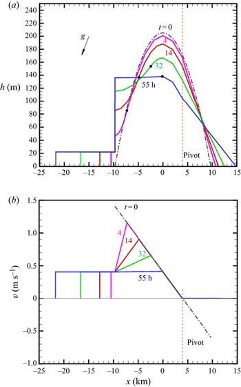
 $t$. This is illustrated in figure 7 and table 1 for the input parameters of the example. The
 $z/x$ ratio of the figure is strongly exaggerated, and the inclination is illustrated by the
 $g$ arrow. The times at which the profiles are presented have been determined by the position of the lower spinup front:
 $x_{Sl}/x_{M0} = 0.75, 0.50, 0.25, 0.1$. The interval between the times increases because the propagation of the spinup front is slower in the thicker fluid near the centre. The pivot is at the fixed
 $x_{\rm \pi}$ where
 $v=0$ prevails.
New model predictions for the parameters of our example, in dimensional form. The  $z/x$ ratio of the plot is exaggerated; the arrow for
 $g$ illustrates the slope. The plots show (a)
 $h(x)$ and (b)
 $v(x)$ at various
 $t$ (corresponding to
 $\tau = 0, 0.67, 2.60, 5.86, 10.16$). The dots on the
 $h$ profiles denote the transition from the spunup to the not-spunup parts in the lower domain.

Predictions for the example. The length scale is  $\sqrt {\mathcal {V}} = 1.15\ \textrm {km}$, and the time scale is
 $(\sqrt {\mathcal {V}}/g')^{1/2} = 686\ \textrm {s} = 0.191\ \textrm {h}$, where
 $\mathcal {V}$ is the half-volume of the initial vein.

We think that these results provide an informative prediction of the motion for a significant time during which a dramatic change of shape and lateral velocity occur. The sharp vertical  $h$ at the front
 $x_{M0}$ in figure 7 looks peculiar. We must keep in mind the distorted
 $z/x$ proportion of this display. This front represents the meeting of the interface Ekman layer with that on the bottom to flow into the merged tail. This merging domain may have a thickness of a few
 $\delta$, with some
 $h_x >0$ inclination. The relevant
 $x$-distances are distorted (compressed) by the aspect ratio that is practical for our figure. We admit that we do not know the details of the flow in this region, but we argue that this does not invalidate the global model. We expect that in practice, the transition between the vein and the tail occurs in some rounded, inclined and smooth domain on the scale of a few
 $\delta$; the sharp transition used in our model is a simplification that is exaggerated strongly by the scaling of the figure.
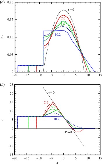
The careful reader may ask why the figures are presented in dimensional form. The main reason is that we could not find a satisfactory scaling that is both simple and informative. Some of the results in dimensionless form, scaled according to § 2.1, are listed in table 1 and in figure 8.
Comparisons between the new model (solid line) and the AW model (dashed line) in dimensionless form for  $\tau = 2.60, 5.86, 10.16$. Parameters are as in our example, with scaling defined in § 2.2.

6. Comparison with the AW model
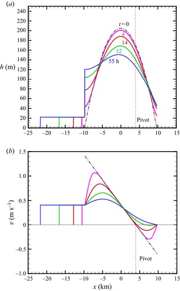
It is of both academic and practical interest to elucidate the qualitative and quantitative similarities and discrepancies between the new and AW models. AW argues that the dynamics of the vein during spinup can be predicted approximately by a ‘minimal model’ formulated as a diffusion equation for  $h(x,t)$ with simple flux conditions at the edges of the interval of solution. Here, we re-derive this model and compare results with our new model. For more details concerning the original derivation, we refer the reader to § 3.3 and figure 2 of AW, and recall that AW discards the Ekman layer on the interface and hence imposes
 $k = 1$ (we will keep the coefficient
 $k$ to facilitate comparisons). Our notation is slightly different; in particular, we use
 $\gamma$ for the slope, and the approximation
 $\tan \gamma = \gamma$.
We use dimensional variables. The components of this model are as follows. The momentum equation is the geostrophic
 \begin{equation} h_x = 2\,\frac{\varOmega }{g'}\,v - \gamma, \end{equation}
the Ekman layer flux and suction/ejection are
 \begin{equation} Q ={-} \tfrac{1}{2} k \delta\,v(x,t), \quad \tilde{w} = \tfrac{1}{2} k \delta\,v_x(x,t), \end{equation}
and the motion of the interface is given by
 \begin{equation} \frac{\partial h}{\partial t} = \tilde{w} = \frac{1}{2} k \delta\,v_x(x,t). \end{equation}
Elimination of  $v$ between (6.1) and (6.3) yields a single equation for
 $h(x,t)$:
 \begin{equation} h_t - k\,\frac {\delta g'} {4 \varOmega}\,h_{xx}= 0. \end{equation}
AW argues that this ‘heat equation’ is valid for the dense fluid ‘in the vein’, i.e. for  $x_A(t) \leqslant x \leqslant x_N(t)$, where
 $A$ is the point where the interface becomes parallel to the bottom (similar to our point
 $M0$). The initial conditions
 $h(x,0)$ are given, which implies that the total initial volume under
 $h(x,t)$ is given (
 $2 \mathcal {V}$).
We note that no balance concerning the lateral  $y$-motion has been used in the derivation of the master equation (6.4). In other words, the governing equation for the dynamics of the ‘minimal model’ makes no explicit use of the spinup process. Indeed, in the new model, (6.3) is applied only to the not-spunup domain. Another reason for concern is the lack of the inclination effect
 $\gamma$ in (6.4). The AW model supposes that these effects can be incorporated by the boundary condition at the edge points
 $N$ and
 $A$.
AW sets these conditions guided by physical expectation and inspection of the interface shape observed in some numerical simulations: at the upslope edge point  $N$,
 $h_x = - \gamma$, and at the downslope edge point
 $A$,
 $h_x =0$. With hindsight, we observe that the spinup analysis of the present investigation supports these boundary conditions, if we identify point
 $A$ with the fixed point
 $M0$. We draw attention to the fact that a boundary condition for
 $h_x$ is tantamount to one for
 $v$; see (6.1). We derived the conditions at the edges from the theoretical argument that the spinup is an outside-in process, and hence at the edges,
 $v$ (and
 $h_x$) attain quickly some fixed values. We now notice that the drainage at point
 $A$ =
 $M0$ and the slope at
 $N$ turn out to be the same in both models. This gives credence to the AW model.
On the other hand, the implementation of these conditions for the diffusion equation (6.4) is problematic. If at point  $N$ the slope is imposed, then the attempt to also impose the physical
 $h=0$ (or
 $h = 5 \delta$) condition produces inconsistencies with the condition at
 $M$. Indeed, the steady-state
 $h_{xx} = 0$ is solved by the line
 $c_1 x + c_2$, which in general cannot satisfy two
 $h_x$ conditions. A serious physical deficiency emerges: in the AW model, the nose
 $N$ does not move upwards. The demonstration is as follows. Using (6.4), and supposing that the interval
 $M$–
 $N$ is fixed as
 $M0$–
 $N0$, we calculate
 \begin{equation} \frac{{\rm d}}{{\rm d}t} \int_M^N h(x,t) \,{{\rm d}\kern0.7pt x} = \int_M^N h_t \,{\rm d}t = k\,\frac{g' \delta }{4 \varOmega }\,[h_x(N) - h_x(M)] ={-} k\,\frac{g' \gamma \delta }{4 \varOmega }. \end{equation}
The result is exactly the drainage from edge  $M0$ derived for the new model; see (5.8). This means that the AW model misinterprets the behaviour of the arrested Ekman layer at
 $N$. The flux stops because
 $v=0$ is imposed there, not because some obstacle is encountered. The artificially arrested flux is accommodated by a local inflation of
 $h(x_{N0},t)$, with no spreadout motion of
 $N$ from
 $N0$. This could be anticipated because (6.3) takes into account only the normal velocity component.
The solution  $h(x,t)$ of the parabolic diffusion (‘heat’) equation (6.4) is obtained numerically (by finite differences). The initial
 $h(x,0)$ in the domain
 $[x_{M0},x_{N0}]$ is given, and the boundary conditions are simple
 $h_x$ (‘heat flux’) fixed values.
Then the numerical  $h(x,t)$ is used to obtain
 $v(x,t)$ from the geostrophic balance (6.1). This elucidates the physical deficiency of this model. Instead of calculating
 $v$ from spinup considerations, the AW model forces this variable to adjust the volume fluxes that support a quasi-steady
 $x$-momentum geostrophic balance. The physical spinup is governed by a hyperbolic equation (see § 4), while the motion predicted by the AW model is governed by the parabolic equation (6.4). This implies that the propagation of the spinup fronts is smeared. Therefore, although the boundary conditions for the diffusion equation are compatible with the spinup process, the predicted spinup motion inside the vein and the displacement of the interface are bound to be distorted by an error that increases with time.
We noted before that the AW model provides the same rate of drainage,  $Q_{CH}$, at point
 $M0$ as the new model. Consequently, it is justified to use the same Ekman-layer tail solution as derived in § 5.4 for the domain
 $M$–
 $M0$.
A quantitative comparison between the models, in dimensionless form, is displayed in figure 8. In this comparison, we used  $k=1.5$ also for the AW model, and we added to this model the tail of § 5.4. The dimensional solutions of the AW model are given in Appendix E.
The qualitative behaviour of the diffusion model interface is in good agreement with the prediction of the new model. As expected, the spreadout of point  $N$ is not captured. Concerning the velocity
 $v(x,t)$ profiles, it is evident that the AW diffusion equation model smears out the spinup fronts predicted by the new model. Therefore, the pivot at
 $x_{\rm \pi}$ with constant
 $v =0$ during spinup is not detected by the AW model. As expected, the disagreement between the prediction of the models increases with time. We conclude that the AW model (supplemented with the tail of § 5.4) is a fair approximation for the beginning of the spinup. The new model is more reliable and provides the spinup behaviour for a longer period of time.
7. Conclusions
We considered the spinup-induced motion of a dense-fluid Cartesian gravity current (GC) on a slope in a rotating system. We developed a new model for the 2.5-D simplified motion (i.e. there is no dependency on the lateral coordinate  $y$, but there is velocity
 $v(x,t)$ in this direction, with
 $x$ in the upslope direction). We elucidated some novel features.
We focused attention on the non-small Rossby number regime (small  $\mathcal {C}$) in which significant deviations from solid-body rotation occur, typical to geophysical currents. The initial situation (
 $t = 0$) of the GC is a natural vein of well-defined geometry symmetric with respect to the midpoint (
 $x = 0$) (but not just a plausible parabola as used in previous investigations), in geostrophic equilibrium, which implies a significant
 $v(x,t=0)$ (counter-rotation about an excentre pivot
 $x_{\rm \pi}$). Then this structure develops rapidly Ekman layers on the bottom and at the interface with the ambient, which drive an internal circulation, which causes the reduction of
 $|v|$ (spinup). We show that the resulting spinup is an outside-in process:
 $v$ at the edges of the vein are reduced first, and from there, spinup fronts propagate towards the fixed pivot point at upslope distance
 $x_{\rm \pi}$ from the midpoint. Therefore, from the beginning, different conditions develop in the up and down sides of the pivot, and the subsequent spinup process is strongly non-symmetric. Typically, the upper part contains less volume and needs a shorter spinup time than the lower part. The flux of the Ekman layers at the upper edge (nose) is arrested by a slowly moving contact point with the bottom, and returned to the pivot in the core (outside the layers). The flux of the Ekman layers at the lower edge is arrested partly and returned, and drained out partly as a fast-moving tail. While both
 $v$ and
 $h$ change, the geostrophic quasi-steady balance between the Coriolis
 $2 \varOmega v$ and gravity
 $g'(h_x + \gamma )$ terms is maintained, because the inertial acceleration terms of the spinup circulation are negligible. We predict that during the major spinup stage, the elongation of the tail is dramatic, but this domain contains only a small part of the initial volume; the main volume performs mostly some deflation–inflation shape adjustments, with little displacement from the initial
 $x$-range. This is in agreement with previous simulations and experiments (Ezer & Weatherly Reference Ezer and Weatherly1990; Wirth Reference Wirth2009).
During the major stage of spinup,  $t \leqslant t_1$, the drainage into the tail is fixed by a choking condition, and the downward propagation of the tail is with constant speed
 $u_M$. The lower part of the vein contracts at the centre and inflates at the drainage point, until a constant
 $h_1$ is attained. Surprisingly,
 $t_1$ does not depend on the slope
 $\gamma$, while
 $h_1 = (2/3)\,h(0,0)$ in general. The reaction of the system to change of the main parameters is summarized in table 2.
Influence of change of the parameters in the first line on the variables of the first column. The arrows  $\uparrow$ and
 $\downarrow$ indicate increase and decrease.

We compared the predictions of our model with those of the simpler AW model, which provides  $h(x,t)$ as a solution of a diffusion equation; the spinup effect is represented only by
 $h_x$ conditions at the edges of the initial vein. There is fair agreement at early times, and perfect agreement concerning the drainage into the tail. The physical spinup is governed by the sharp fronts predicted by a hyperbolic PDE. The diffusive parabolic PDE smears out these fronts with time. This explains the time-increasing discrepancy between the models. Another reason for discrepancy is that the AW model restricts the position of the interface
 $h$ to normal displacement only (inflation and deflation, but not spread out). Therefore, although the AW model captures well the quantitative essentials of the spinup adjustments of the vein, the new model can be considered more reliable physically and of improved coverage.
Another advantage of the present model is the clear-cut identification of patterns, prediction of the initial shape, justification of the boundary conditions, and prediction of the motion. In particular, we derive simple analytical results for the pivot  $x_{\rm \pi}$, propagation of the viscous tail
 $x_M(t)$, and time
 $t_1$. Other results are obtained from algebraic equations.
We admit that our solution is for a quite restricted time,  $t_1$, during which the lateral
 $v$ in the lower part is reduced significantly, but not fully spunup (a few days in ocean systems). However, a significant spreadout occurs during this time. Another uncertainty of the present solution is the stability of the predicted interface close to
 $t_1$. The model contains, explicitly and implicitly, some adjustable constants. The kinematic viscosity coefficient can express either molecular or eddy effects, and this will influence the values of the Ekman-layer thickness
 $\delta$ and the Ekman number. The coefficient
 $k$ expresses the number of Ekman-layer contributions to the spinup shear and flux; while the contribution of the bottom is certain (
 $k=1$), that of the interface is estimated as one-half, thus we used
 $k=1.5$. There are indications that the interfacial Ekman layer decays by diffusion in some circumstances (see Wirth Reference Wirth2011) in which case an intermediate value, such as
 $k=1.25$, may be more accurate. The thickness of the tail, a domain of merged Ekman layers, estimated as
 $5 \delta$, may also need some adjustment when more knowledge is available.
These open issues must be left for future work, including laboratory experiments and direct numerical simulations. We hope that the insights and results presented in this paper will be useful guidelines and comparison data for these future studies. Here, we reiterate that our analysis is focused on a natural vein whose initial profile is determined by release from a lock followed by significant expansion. A similar mathematical model can be derived for a more general ‘forced’ parabolic  $h$ profile in geostrophic equilibrium (note that for a parabola,
 $h_x$ and hence
 $v$ are linear with
 $x$, as in the natural case). However, the details are different, and may require different interpretation; this issue has not been pursued in this study. We also note that the transition between systems with inclined bottom
 $\gamma > 0$ (present solution) and horizontal bottom
 $\gamma =0$ (investigation by Salinas et al. Reference Salinas, Bonometti, Ungarish and Cantero2019) is not clear. A buffer domain of very small
 $\gamma$, in which some features of inclination (like the tail) compete with the tendency of symmetry about the axis predicted by the
 $\gamma = 0$ solution, is expected to exist. We expect that there is some threshold slope
 $\gamma _{tr}$ below which the
 $g' \gamma$ effect is so weak that the symmetric spinup of Salinas et al. (Reference Salinas, Bonometti, Ungarish and Cantero2019) dominates. Since the intrinsic slope of the vein is the aspect ratio
 $\alpha$, we speculate that
 $\gamma _{tr} \approx 0.1 \alpha$. The clarification of this issue must be left to future work. The request that the pivot is inside the vein provides an upper limit to the slope of relevance,
 $\gamma < 2 \alpha$.
Our model discards the motion in the ambient fluid. In realistic circumstances, the ambient is usually confined to a finite height by an open-to-the-atmosphere horizontal boundary, hence volume continuity and dynamic considerations indicate that a return flow (recirculation) is induced in the ambient by the spinup and spreadout motion of the dense layer. This needs a separate study, along similar lines to the recent investigation of Negretti, Tucciarone & Wirth (Reference Negretti, Tucciarone and Wirth2021) for axisymmetric geometry.
Acknowledgements
The author thanks Professor A. Wirth for useful discussions on the topic of this paper.
Declaration of interests
The author reports no conflict of interest.
Appendix A. Dimensional results of initial vein
The dimensionless results for the small  $\mathcal {C}$ case were derived in § 2.4; here we show the dimensional form. Recall that the scaling lengths
 $h_0$ and
 $x_0$ used in § 2.4 are both taken as
 $\sqrt {\mathcal {V}}$ (dimensional), and the lateral velocity is scaled with
 $\varOmega x_0$. Here; the dimensional
 $h, x, v$ are denoted by an asterisk. By straightforward calculations; we obtain
 $$\begin{gather} - x^\ast_M = x^\ast_N = \left ( \frac{3}{4} \right) ^{1/3} \left ( \frac{g' \mathcal{V} }{ \varOmega^2} \right) ^{1/3} , \end{gather}$$
 $$\begin{gather}h^\ast= 2 \left ( \frac{3}{4} \right) ^{2/3} \left ( \frac{ \varOmega^2 \mathcal{V}^2}{g'} \right) ^{1/3} \left [ 1 - \left (\frac{x^\ast}{x^\ast_N} \right ) ^2 \right ], \end{gather}$$
 $$\begin{gather}x^\ast_{\rm \pi} = \frac{g' \gamma}{4 \varOmega^2}, \end{gather}$$
 $$\begin{gather}v^\ast={-}2 \varOmega ( x^\ast{-} x^\ast_{\rm \pi} ). \end{gather}$$
The height/length aspect ratio is
 \begin{equation} \alpha = \frac{h^\ast(0)} { x^\ast_N} = 6^{1/3} \left ( \frac{ \varOmega ^4 \mathcal{V}}{{g'} ^2} \right ) ^{1/3} . \end{equation}
We note the relation
 \begin{equation} \frac{x^\ast_{\rm \pi}}{x^\ast_{N}} = \frac{\gamma}{2 \alpha}. \end{equation}
In geophysical applications,  $\varOmega$ is known, hence the initial vein is prescribed by
 $g'$,
 $\mathcal {V}$ and
 $\gamma$.
Appendix B. The Ekman layers
We present a short derivation and justification of formulas for the flux  $Q$ and suction
 $\tilde {w}$ that appear at the boundary (plate)
 $z=0$ below a large body of fluid in a rotating system. On the plate,
 $u=v=w=0$. Far from the plate, the fluid is an (almost) inviscid ‘core’ whose dominant velocity is
 $v = v(x)$. We use dimensional variables.
Assuming  $\partial /\partial y$ = 0, the steady-state Navier–Stokes (NS) equations read
 $$\begin{gather} u_x + w_z = 0, \end{gather}$$
 $$\begin{gather}u u_x + w u_z ={-} p_x/ \rho + 2 \varOmega v + \nu u_{zz} + \nu u_{xx}, \end{gather}$$
 $$\begin{gather}u v_x + w v_z ={-} 2 \varOmega u + \nu v_{zz} + \nu v_{xx}, \end{gather}$$
 $$\begin{gather}u w_x + w w_z ={-} p_z/ \rho + \nu w_{zz} + \nu w_{xx}. \end{gather}$$
The matching of the core to the no-slip and no-penetration boundary conditions is achieved in a thin layer in which the Coriolis–viscous balance plays a major role, referred to as the Ekman layer. The relevant scale is  $\delta = \sqrt {\nu /\varOmega }$ (see Greenspan Reference Greenspan1968), and the convenient stretched coordinate is
 \begin{equation} \zeta = z/\delta. \end{equation}
We note that when in the core,  $v_{core}$ is linear with
 $x$,
 $u=0$ and
 $w = \textrm {const.}$, the
 $x$-shear terms in (B2)–(B4) are expected to vanish. In this case, and assuming an unbounded domain, the Ekman layer is a part of an exact solution of the NS equation. We present two cases.
B.1. Divergent flow
Let  $v_{core} = \epsilon \varOmega x$, where
 $\epsilon$ is a non-zero constant. In the core,
 $u=0$ and
 $w =\textrm {const}$. We anticipate a solution of the form
 \begin{equation} \left.\begin{gathered} \{ u,v \} = \epsilon \varOmega x\,\{ F(\zeta), G(\zeta) \}, \quad w = \epsilon \varOmega \delta\,W(\zeta), \\ p/\rho = \epsilon \varOmega^2 [ x^2 + \delta^2\,P(\zeta)], \end{gathered}\right\} \end{equation}
where the dimensionless functions  $F,G,W,P$ are of the order unity. Upon substitution, (B1)–(B4) reduce to
 $$\begin{gather} F + W' =0, \end{gather}$$
 $$\begin{gather}\epsilon(F^2 + W F') ={-} 2 + 2 G + F'', \end{gather}$$
 $$\begin{gather}\epsilon (F G + W G') ={-}2 F + G'', \end{gather}$$
 $$\begin{gather}\epsilon W W' ={-} P' + W'', \end{gather}$$
where the prime denotes a derivative with  $\zeta$. The boundary conditions are
 $F(0) = G(0) = W(0) =0$,
 $F(\infty ) = 0$,
 $G(\infty ) = 1$,
 $W(\infty ) =\textrm {const.}$ and
 $P(\infty ) =\textrm {const.}$ (arbitrary). The constant
 $W(\infty )$ is determined by the solution of (B7):
 \begin{equation} W(\infty) ={-} \int_0^\infty F(\zeta) \,{\rm d} \zeta. \end{equation}
This gives the following connections with the core: the flux carried by the Ekman layer is
 \begin{equation} Q = \int_0^\infty u \,{\rm d}z = \epsilon \varOmega x \delta \int_0^\infty F(\zeta) \,{\rm d} \zeta ={-}\epsilon \varOmega x \delta\,W(\infty) ={-} W(\infty)\,\delta v_{core}, \end{equation}
and the suction at the ‘edge’ of the layer is expressed as
 \begin{equation} \tilde{w} = \epsilon \varOmega \delta\,W(\infty) ={-} \partial Q / \partial x. \end{equation}
The coefficient  $\epsilon$ (or rather
 $|\epsilon |$) is the Rossby number of the flow (ratio of inertial to Coriolis accelerations). The inertial terms in (B8)–(B10) are multiplied by this coefficient. The sign of
 $\epsilon$ indicates the swirl
 $v_x$ in the core. Consider the pressure drive in the
 $x$-direction,
 $-p_x/\rho = - 2 \epsilon \varOmega x$. For a negative
 $\epsilon$, the fluid near the plate is pushed outwards and
 $\tilde {w}<0$; for a positive
 $\epsilon$, the fluid is pushed inwards along the plate and
 $\tilde {w}>0$.
The Ekman layer solution of (B7)–(B10) for finite  $\epsilon$ is obtained numerically with the condition at ‘
 $\infty$’ applied at some finite
 $\zeta$. (The solution for
 $P(\zeta )$ is unimportant in the present investigation and will not be shown.) For
 $|\epsilon | \to 0$, the linear Ekman-layer analytical solution
 $G = 1 - \exp (-\zeta ) \cos \zeta$,
 $F = - \exp (-\zeta ) \sin \zeta$ and
 $W(\infty ) = 1/2$ is recovered.
Our main concern is the flow with  $\epsilon = -2$ that appears in the core of the natural vein. The corresponding results are displayed in figure 9. In this case, the Ekman-layer flux, expressed by
 $W(\infty ) = 0.7$, is slightly larger than the linear value
 $1/2$ (based on Coriolis–viscous shear balance, with no inertial terms). Solutions with other values of
 $\epsilon$ indicate that the linear result is a fair approximation for a practical range of
 $|\epsilon |$ that justifies the general simplification for the Ekman-layer transport and suction (
 $\tilde {w}$):
 \begin{equation} Q ={-} \frac{1}{2}\,\delta v_{core}, \quad \tilde{w} = \frac{1}{2}\,\delta\,\frac{ \partial v_{core} }{\partial x}. \end{equation}
For  $\epsilon = -2$, the Ekman-layer results
 $-F, G, W$ versus
 $\zeta$ are shown.

The linear solution, and figure 9 for  $\epsilon = -2$, indicate that the ‘thickness’ of the layer is
 $\approx 3 \delta$, and this value is used in our analysis of the vein unless stated otherwise.
B.2. Non-divergent flow
In the previous subsection,  $v_{core}$ varies linearly with
 $x$. The
 $v=0$ plate generates an Ekman layer with a correspondingly varying
 $Q(x)$ that is accompanied by a non-zero
 $\tilde {w} \sim - \partial Q/\partial x$ volume transport between the layer and the core. The term ‘divergent’ indicates a non-constant
 $Q$ and the presence of a non-zero
 $\tilde {w}$.
The non-divergent counterpart solution with  $w_{core} = 0$ appears when, in the rotating frame,
 $v_{core} = V =\textrm {const.}$ (and
 $u_{core} = 0$). In this case, we expect a constant
 $Q$ in the Ekman layer, and a flow of the form
 \begin{equation} u = u(\zeta),\quad v = v(\zeta),\quad w = 0,\quad p/\rho = 2 \varOmega V x + {\mathrm{ const.}} \end{equation}
Substitution into (B1)–(B4) shows that the continuity equation is satisfied identically, and the inertia terms vanish (the system is linear). The solution subject to the boundary conditions is
 \begin{equation} u ={-}V\,{\rm e}^{-\zeta} \sin \zeta, \quad v = V (1 - {\rm e}^{-\zeta} \cos \zeta), \quad w = 0, \end{equation}
and the Ekman-layer transport is the constant
 \begin{equation} Q = \delta \int_0^\infty u \,{\rm d}\zeta ={-}\tfrac{1}{2}\delta V ={-}\tfrac{1}{2} \delta v_{core}, \end{equation}
while  $\tilde {w} =0$. Note that this result is in full agreement with (B14a,b). In the present case, the inertial terms on the left-hand sides of (B1)–(B4) are identically zero, hence this flow coincides with the solution of the linear
 $\epsilon \to 0$ Coriolis–viscous shear balance.
B.3. Extensions
The results (B14a,b) are a good approximation when the core–boundary interaction is more practical than that used for the exact solutions, in particular time-dependent and with some topography. Suppose that the typical  $x,z$ dimensions of the ‘core’ are
 $L,H$, with
 $H/L$ not large, and the Ekman number is
 $E = (\delta /H) ^2 \ll 1$. Let
 $v(x)$ vary nonlinearly on the
 $L$ scale, and suppose a variation of
 $w$ on the
 $H$ scale that is accompanied by a small
 $u$ (compared to
 $v$). The viscous terms in the NS equations are not identically zero, but are much smaller than the inertial and Coriolis terms, hence the ‘inviscid core’ concept is valid. Overall, it can be shown that the differences of
 $Q$ and
 $\tilde {w}$ from the exact solution predictions turn out to be
 $O(E^{1/2})$. The deviation is also small when (a)
 $v$ varies with
 $t$ on a time scale much larger than
 $1/ \varOmega$, and (b) the bottom boundary slightly varies from
 $z=0$ (with a small local slope). The mathematical details concerning the more general solution are cumbersome, but the qualitative interpretation is straightforward: the new extension contributes small perturbation terms in the NS equations (compared with the ideal flow balances), hence the influence on the results (B14a,b) is small (negligible). We conclude that the use of (B14a,b) with the local and instantaneous
 $v(x,t)$ is justified in the spinup problems considered in this paper.
Appendix C. The inertial term in the geostrophic balance
Consider the  $x$-momentum equation (in dimensional form) during spinup. We argue that
 $\textrm {D}u/\textrm {D}t$ is negligible as compared to the
 $g' \gamma$ term. We use an order of magnitude argument. We have
 $\textrm {D}u/\textrm {d}t \sim U/T$. During spinup,
 $U \sim \varOmega x_{N0} \delta /h_{00} = E^{1/2} \varOmega x_{N0}$ and
 $T \sim x_{N0}/U$, where
 $h_{00}=h(x=0, t=0)$ and
 $E = (\delta /h_{00})^2$. Consequently, we estimate
 \begin{equation} \frac{U}{T g'} = \frac{U^2}{h_{00} g'} = E\,\frac{\varOmega^2 x_{N0}}{g'} = E \mathcal{C}^{4/3}. \end{equation}
In our example, the estimate (C1) is of the order of  $10^{-4}$, much smaller than
 $\gamma = 0.017$. This is typical of geophysical systems. This justifies the use of the quasi-steady geostrophic balance (5.2) during spinup. It is also evident that the term (C1) is much smaller than the first term on the right-hand side of (5.2).
Appendix D. Natural vein for large $\mathcal {C}$ (small Rossby number)

Here, we use dimensionless variables; see § 2.2, with  $x_0= h_0 = \sqrt {\mathcal {V}}$. The geostrophic adjustment ends with a steady-state structure
 $u=0, v_t=0$, but non-trivial
 $h(x), v(x)$. To calculate these variables, we combine (2.7) with (2.4) (in steady state) into
 \begin{equation} v_{xx} - 4 \mathcal{C}^2 v ={-}2 \gamma, \quad h = 1 + \tfrac{1}{2} v_x. \end{equation}
The boundary conditions are  $h=0$ at the edges
 $x_M,x_N$, and given total volume 2.
The solution  $v(x), h(x)$ is a combination of
 $\exp (\pm 2 \mathcal {C} x)$ (plus a constant), and the large
 $\mathcal {C}$ implies that a sharp variation (like a boundary layer) appears at the edges
 $x_M$ and
 $x_N$. After some manipulations and matching with the boundary conditions, we find that the leading terms are
 \begin{equation} -x_M = x_N = 1 + \frac{1}{2 \mathcal{C}}. \end{equation}
Recall that  $1/(2 \mathcal {C})$ is the Rossby radius (dimensionless). The initial spreadout of the vein with large
 $\mathcal {C}$ is exactly one Rossby radius.
In the upper part,  $0 < x \leqslant x_N$,
 \begin{equation} h(x) = 1 - \exp [ 2 \mathcal{C} (x - x_N) ], \quad v = \frac{\gamma}{2 \mathcal{C}^2} - \frac{1}{2 \mathcal{C}} \exp [ 2 \mathcal{C} (x - x_N) ]. \end{equation}
In the lower part,  $x_M \leqslant x <0$,
 \begin{equation} h(x) = 1 - \exp [ 2 \mathcal{C} (x_M - x) ], \quad v = \frac{\gamma}{2 \mathcal{C}^2} + \frac{1}{2 \mathcal{C}} \exp [ 2 \mathcal{C} (x_M - x) ]. \end{equation}
There is symmetry of  $h(x)$ about
 $x=0$, but again not of
 $v(x)$.
Since in this case the change from the initial  $h=1$ and spread
 $[-1,1]$ is small, it is convenient to chose the scalings
 $h_0$ and
 $x_0$ in accordance with the observed vein, if it is of this type. The change of scaling variables does not affect the form of the results, with the exception that
 $\gamma$ should be multiplied by
 $x_0/h_0$. Evidently, the numerical value of
 $\mathcal {C}$ changes. The spinup of this vein needs an investigation different from that of the small
 $\mathcal {C}$ case because here
 $h_x =0$ in the main domain from the beginning. The instability trends are also different (baroclinic rather than shear, because
 $v$ is small). This flow is beyond the scope of this paper.
Appendix E. Results of the AW model
The plots of figure 10 are the counterpart of the new model results of figure 7. The original AW model does not predict the tail; here, we added the tail of § 5.4. A comparison between the models is given in figure 8.
AW model predictions, details as in caption of figure 7.