




No CrossRef data available.
JOIN MINIMUM COST QUEUE FOR MULTICLASS CUSTOMERS: STABILITY AND PERFORMANCE BOUNDS
Published online by Cambridge University Press: 01 October 2004
Abstract
We consider a system of K parallel queues providing different grades of service through each of the queues and serving a multiclass customer population. Service differentiation is achieved by specifying different join prices to the queues. Customers of class j define a cost function ψij(ci,xi) for taking service from queue i when the join price for queue i is ci and congestion in queue i is xi and join the queue that minimizes ψij(·,·). Such a queuing system will be called the “join minimum cost queue” (JMCQ) and is a generalization of the join shortest queue (JSQ) system. Non-work-conserving (called Paris Metro pricing system) and work-conserving (called the Tirupati system) versions of the JMCQ are analyzed when the cost to an arrival of joining a queue is a convex combination of the join price for that queue and the expected waiting time in that queue at the arrival epoch. Our main results are for a two-queue system.
We obtain stability conditions and performance bounds. To obtain the lower and upper performance bounds, we propose two quasi-birth–death (QBD) processes that are derived from the original systems by suitably truncating the state space. The state space truncation in the non-work-conserving JMCQ follows the method of van Houtum and colleagues. We then show that this method is not applicable to the work-conserving JMCQ and provide sample-path-based proofs to show that the number in each queue is bounded by the number in the corresponding queues of these QBD processes. These sample-path proof techniques might also be of independent interest. We then show that the performance measures like mean queue length and revenue rate of the system are also bounded by the corresponding quantities of these QBD processes. Numerical examples show that these bounds are fairly tight. Finally, we generalize some of these results to systems with more queues.
Information
- Type
- Research Article
- Information
- Probability in the Engineering and Informational Sciences , Volume 18 , Issue 4 , October 2004 , pp. 445 - 472
- Copyright
- © 2004 Cambridge University Press
1. INTRODUCTION
We consider a system of K parallel queues providing different grades of service in each of the queues to a multiclass customer population with J classes. Service differentiation is achieved by different join prices for the queues and service rates in them. A join price ci is prescribed for service from queue i. Customers also incur a congestion cost due to, say, delays. These two costs are reflected in the customers of class j defining a cost function ψij(ci,xi) for service in queue i when the join price is ci and congestion is xi. Obviously, ψij(ci,xi) should be increasing in ci and xi. Let c = [c1,…,cK]T be the price vector and x(t) = [x1(t),…,xK(t)]T be the queue length vector at time t. The queue system posts both c and x(t). A customer of class j arriving at time t calculates its cost for service from queue i for i = 1,…,K and joins that queue for which the cost is minimum. This queuing system will be called the “join minimum cost queue” (JMCQ). A customer class is determined by the set {ψ1j(·,·),…,ψKj(·,·)}. Thus, the JMCQ is a generalization of the well-known join shortest queue (JSQ) system.
An important motivation for this problem is to price quality of service in the Internet through an access charge. Specifically, we target the multiclass service system as defined by the DiffServ model of the IETF of Blake et al. [2]. In DiffServ, the per hop behaviors are implemented by means of appropriate scheduling mechanisms and users select the service class that best fits its requirements of quality. The JMCQ system described above can be seen to be amenable to this service as follows. A set of K service classes is defined. The total link capacity μ is divided among the K queues such that queue i is serviced at rate μi, μi > 0 with

. The price for service and the congestion in queue i (ci and xi, respectively) are posted. The instantaneous queue length or the unfinished work in the queues are examples of congestion information. In the extreme, each packet can calculate its cost for service from each class and take service from the queue that minimizes the cost.
The applicability of a multiclass service system to pricing quality of service in the Internet has been recognized for quite some time now. For example, Odlyzko [16] argues that the pricing scheme in the Paris Metro could be extended to pricing differential quality in the Internet. The network is partitioned into multiple logical networks with identical resources and the service in each partition is priced differently. If occupancy information in each partition is provided, prices would act as a control to provide differential service. This pricing model is called the Paris Metro pricing (PMP) scheme. Jain, Mullen, and Hausman [10] report an analysis to model the profitability of this pricing scheme. Gibbens, Mason, and Steinberg [9] describe more results. The PMP, as it is proposed, is a non-work-conserving scheme with the link capacity statically partitioned among the service grades. In Dube, Borker, and Manjunath [6], a work-conserving version of PMP called the Tirupati scheme is proposed. In this scheme, if there are no customers in a queue, the capacity allocated to it is distributed among the nonempty queues. This scheme takes inspiration from the queue management scheme in Tirupati, a major pilgrimage center in southern India, where it has been operating with remarkable efficiency for quite some time now. Dube et al. [6] analyzed the social optimality of the Tirupati pricing model and showed that the difference between the social cost of the optimally priced system and that of the Tirupati system is Cε for some constants C and ε. Another, more practical, contribution of Dube et al. [6] was dynamic pricing using a dynamic programming equation and a reinforcement-learning-based online pricing algorithm. A simple learning-scheme-based pricing mechanism to dynamically determine the join prices to provide a specified average grade of service from each queue is analyzed and described in Borkar and Manjunath [3]. A preliminary comparative analysis of the Tirupati and PMP queuing systems is presented in Manjunath, Goel, and Hemachandra [12], where it is shown numerically that the revenue rate is neither monotonic in nor a convex function of the prices. Refer to Falkner, Devetsikiotis, and Lambadaris [7] for a recent survey of Internet pricing.
Another application of the JMCQ is in pricing service at popular websites. There are a number of websites that now offer a faster service for a charge. The service offering is the same for the free and the priced version and the user pays for faster access.
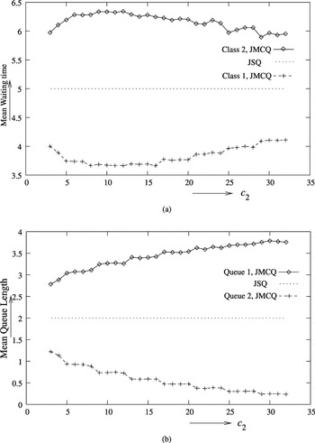
We now show by way of a numerical example how pricing can selectively improve the grade of service of specific classes in a multiclass environment. Consider customers that use a convex combination of the join price and the expected waiting time as the cost [i.e., ψi(c,x) = (1 − ai)x + ai c]. Consider a work-conserving queue with two classes of customers with a1 = 0.8 for a delay-sensitive class and a2 = 0.3 for a price-sensitive class. Let the arrival rate and mean service time of both classes be the same. In a work-conserving JSQ system, both classes would get the same grade of service. To provide a better grade of service to the delay-sensitive class, let one of the queues prescribe a join price, say p. For an arrival rate of 0.4 for both classes of customers and a service rate of 0.5 in both the queues, Figure 1a shows the mean waiting time for each class and Figure 1b shows the mean queue lengths. Observe the significant decrease in mean delays for the delay-sensitive customers. See [19] for more detailed numerical results.

Plots illustrating the differentiated service provided by JMCQ. (a) Mean waiting time of customers of different classes for the work-conserving JMCQ system compared with that of the JSQ system. (b) Mean queue lengths for the work-conserving JMCQ compared with the mean queue length in the JSQ system.
In this article, we analyze the JMCQ applied to one link of a network or to a web service under a static pricing regime. After describing the model assumptions and notations in the next section, we first derive stability conditions for the queues under both the work-conserving Tirupati JMCQ and the non-work-conserving PMP JMCQ in Section 3. In addition to the usual performance measures of moments of the delay and queue length, the revenue rate for the queue system and the social cost are important measures. JMCQ is a generalization of JSQ and one can expect that it will be hard to obtain exact results. We focus on computable bounds for the performance measures.
There is considerable literature on JSQ. Boxma, Koole, and Liu [4] presented a recent survey of the results for JSQ. van Houtum, Zijm, Adan, and Wessels [20] gave a methodology for obtaining computable bounds for performance measures of JSQ that are related to mean rewards of the associated Markov chain. van Houtum, Adan, Wessels, and Zijm [21] considered a generalization of JSQ, where jobs of a class join the shortest of the queue that is capable of serving it. They proposed computable bounds for useful performance measures. For asymptotic results, Foley and McDonald [8] presented a recent example. In Section 4, we derive computable bounds for the performance measures mentioned above. For the non-work-conserving PMP model, we show how the methodology of [20] can be adopted for obtaining computable bounds for revenue rate and stationary mean number in each queue. We next observe that this methodology is not suited for the work-conserving Tirupati model. Our main result here is to show that the state space can be truncated in such a way as to form a quasi-birth–death (QBD) process in which the number in each component of the QBD processes gives bounds for the number in the queues of the JMCQ model. We show this by sample-path arguments and see that these bounds can be made fairly tight. We provide two numerical examples in Section 5 and conclude with discussions on generalization in Section 6.
2. MODEL DESCRIPTION
Without loss of generality, we let the queue join prices be ordered such that c1 ≤ c2 ≤ ··· ≤ cK. Customers of class j arrive according to a Poisson process of rate λj and these arrival streams are independent. Denote

, so that λ is the total customer arrival rate into the system. An arrival at time t selects the queue to join as described in the previous section. Ties in cost are awarded to the queue with the lowest join price.
The service requirements are assumed identical among the classes. This assumption is not unreasonable in modeling web service, in the urban transport system, in the Paris Metro system, or in the queue at Tirupati. It is especially not an unreasonable assumption in the context of Internet bandwidth, where a fixed access charge is the most prevalent charging mechanism.
The service times are independent and identically distributed (i.i.d.) exponential with unit mean. The total service capacity is μ and is partitioned among the queues as follows. The non-work-conserving system has static partitioning and queue i is served at rate μi,
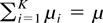
. The work-conserving system uses the generalized processor sharing model of Parekh and Gallager [17] with weight wi for queue i; that is, at time t, queue i receives service at rate μi(t), where
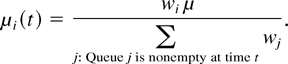
The cost of service from queue i for a class j customer, ψij(·,·), will be assumed to be a convex combination of the queue length and join price of the ith queue. (Because the service times are exponential, the expected waiting time from queue i is equal to the instantaneous queue length at the arrival epoch.) This is a simple and effective way of capturing price and delay sensitivities for different classes of customers. Thus, in the following, ψij(·,·) will be of the form

The aij will be called the delay sensitivity of class i with respect to queue j. We immediately simplify the model by letting aij = ai for j = 1,…,J; that is, the delay sensitivities are independent of the queue. Thus, the ψij(·,·) will be given by

This is a reasonable assumption when, for example, the service rate is the same in both queues.
In much of the rest of the article, we will consider a system with two queues, K = 2, and two customer classes, J = 2. Without loss of generality, we assume a1 > a2; that is, class 1 customers are more delay sensitive than the class 2 customers, who can be called price sensitive. We indicate generalizations to systems with K > 2 and J > 2 in Section 6.
We now introduce the concept of an attractor line which will help in a better understanding of the system. First, consider the system with only one class of customers, say class 1. Recall that we let c1 < c2. On the x1–x2 plane, an “attractor” line can be defined such that an arrival to the system when it is in a state on the left of this line will join queue 1. Similarly, an arrival to the system when it is in a state on the right of the attractor line will join queue 2; that is, arrivals tend to move the system toward the attractor line. For ψj(·) as above, the attractor line is defined by
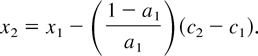
In a JMCQ system supporting multiclass traffic, an attractor line is defined for each class.
3. STABILITY ANALYSIS
We consider the stability of the queuing systems in terms of the ergodicity of the associated Markov chains.
3.1. Non-Work-Conserving PMP System
Let x(t) = [x1(t),x2(t)]T be the state of the system at time t, where xi(t) is the number of customers in queue i at time t in the non-work-conserving JMCQ. {x(t)}t≥0 evolves as an irreducible continuous-time Markov chain (CTMC) over the state space

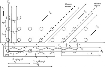
. The transition rates for {x(t)}t≥0 are as shown in Figure 2. Let {xn}n≥0, n an integer, be the jump chain (see, e.g., Asmussen [1] or Norris [16]) derived from {x(t)}t≥0 and let {px:x′} be its transition probabilities.

The transition rates for {x(t)}t≥0, the CTMC for the non-work-conserving queue system. Partitions A1,…,A5 and F used in the stability analysis of Theorem 1 are also shown.
Lemma 1: If λ1 + λ2 > μ1 + μ2, then both the jump chain {xn}n≥0 and {x(t)}t≥0 are transient.
Proof: Define

to be h(x) = ((μ1 + μ2)/(λ1 + λ2))(x1+x2). When λ1 + λ2 > μ1 + μ2, we have h(x) bounded, h([0,0]) = 1 > h(x),x ≠ [0,0]. Also, for any state

,

can be verified. Hence, from Theorem 2 of Mertens, Samuel-Cahn, and Zamir [13], it follows that the jump chain is transient. From Theorem 3.4.1 of Norris [15], the lemma now follows. █
Theorem 1: {x(t)}t≥0 is positive recurrent if λ1 + λ2 < μ1 + μ2.
Proof: For uniformizable CTMCs, Kingman [11] showed that Foster's criteria can be stated as follows. An irreducible CTMC is positive recurrent if and only if there exist nonnegative yx such that


As in Kingman [11], we use a quadratic Lyapunov function yx := x12 + x22. As with a typical queuing system, it can be easily verified that (1) holds when λ1 + λ2 < μ1 + μ2. The finite number of states referred to in (2) will include set F (see Fig. 2) and some more states identified below.
In region A1 of the state space, (2) reduces to requiring −λ + 2x2 μ2 − μ2 ≥ 1, which holds for all sufficiently large x2. A similar relation is satisfied in A2 for all but finitely many x1. In region A3, (2) simplifies to

Let ε1 := μ1 − λ2 and ε2 := μ2 − λ1. If εi > 0,i = 1,2, then (3) is true for all large x1 and x2. Suppose ε1 > 0 and ε2 < 0 such that ε1 + ε2 = μ − λ =: δ > 0. λ and μ are as defined earlier. Then, (3) reduces to

where d := λ1 = λ2 + μ1 + μ2. Since the attractor lines have positive x1 intercepts, we have x1 > x2 and, hence, (4) is valid for all large x1 and x2. Finally, suppose ε1 < 0 and ε2 > 0. As in the previous case, (3) reduces to

For a given x2, we have that x2 ≤ x1 ≤ x2 + k2, where k2 is the intercept of the class 2 attractor line and, hence, (5) can be written as

which is true for all large x1.
In region A4, (2) becomes 2x1(μ1 − λ1 − λ2) + 2x2 μ2 − d ≥ 1. Now, let ε := μ1 − (λ1 + λ2) and ε + μ2 = (μ1 + μ2) − (λ1 + λ2) =: δ > 0. If ε ≥ 0, then (2) holds for all large x1 and x2. Suppose ε < 0; then, (2) reduces to

For that part of A4 with x2 ≥ x1, (6) holds for large values of x1 and x2. If x1 > x2 in A4, we have x1 − x2 < k1, where k1 is the x1 intercept of the class 1 attractor line. In this case, (6) can be reduced to

which holds for all large values of x1 and, hence, (2) is true in A4 also.
In region A5, (2) reduces to 2x1μ1 + 2x2(μ2 − λ1 − λ2) − d ≥ 1. If μ2 ≥ λ1 + λ2, we have the desired inequality for all but finitely many states of A5. On the other hand, if μ2 < λ1 + λ2, let ε := λ1 + λ2 − μ2 and μ1 = ε + δ for some δ > 0. In this case, (2) can be written as

and (2) follows from the fact that x1 > x2. █
3.2. Work-Conserving Tirupati System
Recall that in the work-conserving system the capacity of an empty queue is distributed among the nonempty queues. Let

be the state of the system at time t, where

is the number of customers in queue i at time t. Under the model assumptions,

evolves as an irreducible CTMC over the state space

, also denoted by

. The transition rates for

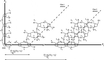
is as shown in Figure 3.

The transition rates for , the CTMC for the evolution of the work-conserving JMCQ. Observe that the departure rates for states on the axes are μ = μ1 + μ2.
Consider a process

such that

.

satisfies the conditions for Theorem 2.4 of Bremaud [5, Chap.9] and is, hence, identical to an M/M/1 queue with arrival rate λ1 + λ2 and service rate μ1 + μ2. Thus, from the stability conditions of the M/M/1 queue, we can state the following theorem.
Theorem 2:

is
1. transient iff λ1 + λ2 > μ1 + μ2,
2. positive recurrent iff λ1 + λ2 < μ1 + μ2,
3. null recurrent only iff λ1 + λ2 = μ1 + μ2.
4. PERFORMANCE BOUNDS
We first define the performance measures of interest. Consider the non-work-conserving system. Let nj(t) be the number of class j arrivals in (0,t) and n(t) := n1(t) + n2(t). Let the kth arrival join queue δk, δk ∈ {1,2}. The revenue rate,

, of the system is defined as

Here, I(·) is the indicator function, with the usual meaning of taking a value one if the argument is true and zero otherwise.
An arriving customer of class j joining queue i when queue i has xi customers incurs a cost of ψj(ci,xi). The rate of social cost

for class j is defined below. Let kj be the kth arrival of class j and let its arrival time be tkj. Then,

The social cost for the system

can be similarly defined. Also, xi will denote the mean queue length in queue i and x the mean number in the system obtained as time averages. Similarly, we will denote the mean waiting time of a class j customer by wj, which is obtained as a customer average.
The corresponding measures for the work-conserving system will be

.
4.1. Non-Work-Conserving System
Consider the PMP system first. Define δxj to be the queue that an arriving class j customer to state x will join. For example, when the system is in state x = [x1,x2], δx1 = 1 if ψj(c1,x1) ≤ ψj(c2,x2) and δx1 = 2 otherwise. The transition rate matrix Qx = {qx:x′} is easily determined. The previous section contains sufficient conditions for the ergodicity of this Markov chain, and in the following, we assume that they hold. Let π = {πx} be the stationary distribution of this Markov chain. The revenue rate

and the per class rate of social cost are obtained from the Law of Large Numbers (see Serfozo [18]) as follows:


Closed-form expressions for

are difficult to obtain and we look for approximate results in the form of computable bounds. First, consider the revenue rate,

. We use the framework of van Houtum et al. [20] to obtain computable bounds by considering systems on a truncated state space.
Denote the original non-work-conserving JMCQ system defined over the state space

by

and let {x(t)}t≥0 be the CTMC of this system. Further, let {xn}n≥0 be the corresponding uniformized jump chain of the

system obtained from a uniformizing Poisson process of rate d := μ1 + μ2 + λ1 + λ2 (see Bremaud [5]). Since the steady state distribution is the same both in the CTMC and its corresponding uniformized chain, we work with {xn}n≥0 in the rest of this section.
Let

be the indicator variable which captures the queue from which ith customer has departed and let

be the number of departures from the system up to time t. Let

be the revenue rate accrued if each customer is charged while departing from the system (instead of charging while entering the system). We claim that

almost surely. We first note that the following two limits exist almost surely:
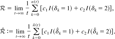
Let {τn}n≥0 ↑ ∞ be the sequence of the end of busy periods of the stable system (i.e., return times to 0). Then, for the system that starts empty,

for each n. Since

exist, we can divide the above by τn and take limits along this subsequence, to have

almost surely. So, (7) can be written as, almost surely,

We rewrite (9) as
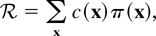
where c(x) is the revenue rate in state x given by
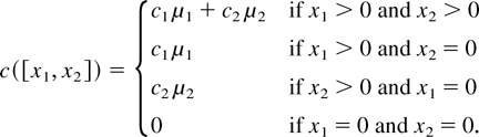
Following [20], we now establish precedences between states of {xn}n≥0. These precedences are defined on the basis of the n-period revenue vn(x), which denote the expected revenue in the first n ≥ 0 periods when starting from state x. We say that the state

has precedence over state

, if m and n satisfy the precedence relation

Denote the unit vectors [1,0] and [0,1] by e1 and e2, respectively. We claim that state m has precedence over its neighboring states m + e1 and m + e2 for all

. Also, note that the ≤ operation is transitive.
Let P be the set of all ordered pair of states (m,m + e1) and (m,m + e2),

. We want to prove for all n = 0,1,2,…,

We use induction over n to prove (12). Taking n = 1 in (12) leads to

We can easily verify that (13) holds. Assume that (12) holds for n and we prove it from n + 1. To establish (12) for n + 1, we have to show for each (m,n) ∈ P,
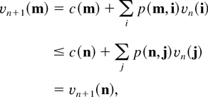
where p(m,n) denotes the corresponding transition probabilities of {xn}n≥0. From (13), it suffices to show that

In the non-work-conserving system, we can check (15) for all (m,n) ∈ P. A convenient method of checking is by grouping terms corresponding to the same event (such as an arrival or departure). The attractor lines of the different customer classes divide the state space into many regions, and the transition probabilities depend on the region in which the state is located. Thus, we will have to verify (15) for the various regions. We illustrate this for the region A3 in Figure 2. Let n = m + e1 in (15). The left-hand side of (15) is

and the right-hand side is

Therefore, proving (15) implies proving

This is true because each term in the above inequality is nonnegative from the induction hypothesis. Similarly, we can verify (15) for the remaining regions.
Now, we propose two truncated systems and prove that the revenue rates in these systems act as bounds for the revenue rate in the

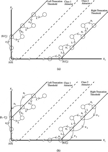
system. To motivate the truncation, we argue that πx becomes very small for states x away from the attractor lines; hence, most of the probability mass of {πx} is concentrated between the attractor lines and close to it and a state space truncated at some distance from the attractors will provide a good approximate solution. In the following, we show that if the truncation is done such that the transition from the states on the threshold lines are suitably modified, we can obtain bounds on the performance measures defined earlier, which can be made fairly tight. Specifically, we will consider the state space of the JMCQ truncated to contain only those states for which Tl ≤ x1 − x2 ≤ Tr, where Tl and Tr are integers with Tl ≤ 0 and Tr ≥ ((1 − a2)/a2)(c2 − c1) > 0. Tl and Tr will be called the left and right truncation thresholds, respectively. Denote by

the state space obtained after truncation. Also, let

be the states on the left threshold line (x1 − x2 = Tl), except the state [0,|Tl|]. Further, let

be states on the right threshold line (x1 − x2 = Tr), except the state [Tr,0], and

. Figure 4 shows this truncation.

The truncated state space for the systems. The modified transitions rates for states on are shown. The transition rates for the states between the truncation lines are the same as that of system shown in Figure 2. (a) Transition rates for the system. For states in , transitions due to departures from queue 1 (2) are disallowed. (b) Transition rates for the system. For states , there is a diagonal transition with a rate μ1 (μ2).
Denote the original work-conserving JMCQ system defined over the state space

by

. We define systems

over

as follows. For system

, let Q(u) = {qx:x′(u)} be its transition rate matrix obtained from Q as follows:
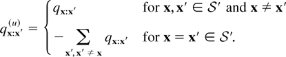
From the above, for

an arrival will move

toward the attractor line of its class (the attractor lines of all the classes are included in the truncated state space) and will not cause the system to go out of

. For

, a departure from queue 1 is disallowed, whereas for

a departure from queue 2 is disallowed to keep the system in

. Other transition rates are the same as that in

.
The transition rate matrix Q(l) = {qx:x′(l)} for system

is obtained from Q as follows. As with

, the transition rates from states

are the same as that in

. The departures from the states on the threshold lines are modified such that a departure from one queue that might lead to a state out of

will take away one more customer from the other queue also and, hence, keep the system state in

.
Let πx(u) and πx(l) be the stationary distributions of

, respectively. For the following, we will assume that both of these systems are stable and, hence, that their stationary distributions exist. We will discuss the stability of these systems in Section 5.
Let {xn(u)}n≥0 and {xn(l)}n≥0 be the uniformized jump chains of the

systems obtained from a uniformizing Poisson process of rate d := μ1 + μ2 + λ1 + λ2. For these systems, we can write the revenue rate as
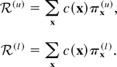
In our truncation model, we observe that {xn(u)}n≥0 is obtained by redirecting transitions to preceding states and {xn(l)}n≥0 is obtained by redirecting transitions to succeeding states. Thus, from Theorem 1 in [20], we have the following result.
Theorem 3: If systems

, start empty at t = 0, we have

Now, consider the bounds on the mean queue lengths. Choosing c(x) = x1 in (10), we get the expression for the mean number in queue 1: x1. Similarly, choosing c(x) = x2 gives the expression for the mean number in queue 2: x2. Using induction, we can again prove that m precedes m + e1 and m + e2. Let xi(u) and xi(l) be the mean queue lengths in queue i for the

systems, respectively. Thus, we have the following result.
Theorem 4: Let xi, xi(u), and xi(l) exist for i = 1,2. Then,

Further, if we take c(x) = 1 for x1 > M and zero otherwise, where

, then [sum ]x c(x)πx is the tail probability that the total number of customers in queue 1 exceeds M. As a result, the stationary number in queue 1 in the

system is stochastically bounded between the stationary number in queue 1 of the

systems. We have a similar result for the stationary number in queue 2 in the

system. In fact, we can show that if all systems start in the same feasible state, say (0,0), then at any jump epoch, the number in a queue of the

system is stochastically bounded by the number in the corresponding queues of the

systems.
Remark 1: We can also show that the number in each queue of

almost surely bound the number in the

system at every jump epoch. The proof technique is similar to that used to show such bounds for the work-conserving system, which we discuss next.
4.2. Work-Conserving System
We now obtain results similar to those in the previous subsection for the work-conserving system. We will use the same notation for the parameters and performance measures as in the previous subsection except that they will have a tilde to differentiate them from the corresponding variables of the non-work-conserving system. For example,

will be the queue occupancy in queue i at tk.
We first show that for the work-conserving system, we cannot obtain the bounds for the performance measures by proceeding exactly as in the previous section and applying the method of [20]. To see this, consider bounds for the revenue rate. As in the non-work-conserving system, we can write the revenue rate for the

system as

This can be written in terms of μ as
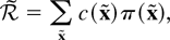
where

represents the cost per period in state

given by
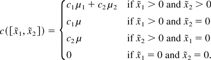
In the work-conserving system, the cost function on the axes is forced to be ci μ, where μ = μ1 + μ2. For our truncation model to yield bounds for the revenue rate, the precedence relation mentioned in the previous subsection must hold here also; that is, the state

must precede the states

for all

. Suppose that the above-mentioned precedence relations hold. Let

be the set of all

. Then, for all t = 0,1,2,…,

Specifically, this must hold for t = 1. Taking t = 1 in (19) leads to

However,

contradicting (20). Thus, the assumed precedence relations are false and the proposed truncation model will not yield bounds using the techniques in [20]. We take an alternate approach to prove the bounds for the revenue rate of the

system.
4.3. Sample-Path Approach
Let

be the CTMC of the

systems, respectively. Let

be the corresponding uniformized jump chains of the

systems, respectively, obtained from a uniformizing Poisson process of rate d := μ1 + μ2 + λ1 + λ2 (see [5]). Now, consider the uniformized systems

evolving in parallel and driven by the same event sequence determined by the Poisson process. We now present a forward induction type of proof (see Walrand [22, Chap.8]) to show that system

(resp.

) componentwise dominates

(resp.

) for all n.
Let t1 < t2 < t3 < ··· be the event epochs of the uniformizing Poisson process. Every jump of this Poisson process corresponds to either an arrival of class j, j = 1,2 with probability λj /d, or a potential service completion from queue i, with probability μi /d. An arrival will join the queue that minimizes its cost, possibly different queues in different systems. The work-conserving property leads to the following queue dynamics at potential service completion instants. A potential service completion time from queue i is an actual service completion from that queue if it is nonempty, and it is an actual service completion in the “other” queue if queue i is empty and the other is nonempty. Because the service and interarrival times are exponentially distributed, we just disallow departures when actual departures are not possible at potential departure times. Let

be the state of

“just after” tn and let

be the sample path of

up to time tN+. Reference [22] has more details on the development of the sample paths. Denote the evolution paths by

in the

system and by

in the

system and let

.
Theorem 5: If the system starts empty at k = 0, then for any k ≥ 0,
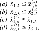
Proof: Assume that (a) and (b) have not failed till tk. Both (a) and (b) cannot fail for the first time simultaneously and we consider the events that might lead to them failing separately. We will consider (a) alone first. For (a) to fail before (b) at tk′+1, we require that

. We consider the possible events at tk′ with this condition. If the event at tk′ is a potential departure, the following subcases arise:
1. Potential departure from queue 1: Because

will behave identically with respect to queue 1 when

. If

, a departure from queue 1 is disallowed in

and allowed in

, and (a) is maintained.
2. Potential departure from queue 2:

is necessary to cause an actual departure from queue 1. By assumption that (b) has not failed until tk′,
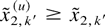
implying

.

will behave identically with respect to queue 1.
Now, consider the case when the event at tk′+1 is an arrival. For (a) to fail, the arrival must join queue 1 in

and queue 2 in

. For this to happen,

must be on the right-hand side of the attractor line for the class of the arrival, and

must be on its left-hand side. This is clearly not possible because

and the attractor line has a positive slope.
Similar arguments show that (b) cannot fail before (a) at tk′+1.
Now, consider (c) and (d). Once again, they cannot fail for the first time simultaneously. We proceed as above and look at events at tk′+1 when

, which is required for (c) to fail for the first time and before (d) at tk′+1.
As previously, first consider a potential departure at tk′:
1. Potential departure from queue 1: Because

will behave identically with respect to queue 1 when

. If

, an actual departure takes place from both the queues in the

system and the inequality is maintained.
2. Potential departure from queue 2:

is necessary to cause an actual departure from queue 1 in

. However, by assumption that (d) had not failed until
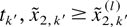
and, hence,

.

will behave identically with respect to queue 1.
For an arrival of class j at tk′+1, arguments identical to that from the first part are used to show that (c) does not fail at tk′+1.
Similar arguments are constructed to show that
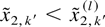
could not have happened at tk′ and, hence, (d) could not have failed before (c) for the first time at tk′+1. █
Let
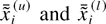
be the mean queue lengths in queue i for the

systems, respectively. Also, let

be the mean waiting times in queue i of the

, and the

systems, respectively.
Theorem 6: Let

exist for i = 1,2. Then,
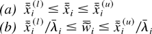
for i = 1,2, where λi is the long-run arrival rate into queue i in the

system.
Proof: From Wolff [23],

systems are regenerative and, hence, the mean queue lengths are also time averages. Hence,

Similarly we can prove the left half of (a).
From Little's law, we write (b) as

Dividing throughout by λi, we get (b). █
Now, we find the bounds on the revenue rate. In this case, we choose Tl = 0 and, hence, the left truncation threshold is the line

. The revenue processes in

are modified as follows. The

systems will earn revenue exactly like the

system, except for the following cases. We stipulate that when the system is in a state in

will “gain revenue” (c2 − c1) and

will “lose revenue” c1 according to the rate μ2. When the system is in a state in

, only

will “lose revenue” c2 according to the rate μ1. Let

be the revenue rates so earned in systems

, respectively. Then, from the Law of Large Numbers,

Observe that the expressions for

are similar to that for

in (17) except that they are defined on the corresponding

systems, respectively, and the “revenue earnings” are modified for the states on the threshold line as discussed in the previous paragraph. Let

denote the cumulative revenue in

, respectively, until time tN.
Theorem 7: If the

systems start empty at time t = 0, then for all N ≥ 0,

Proof: Let
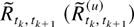
be the revenue “earned” in the transition at tk+1 from

in the

system. We can write the left-hand side of Eq. (22) as

We will show that the following holds for all tk, the epochs of the uniformizing process:

For an arrival at

. A similar expression is written for

and (24) is satisfied. Now, consider potential departures. We consider four cases corresponding to the state of the queues in

.
Case 1: Both queues are empty. Irrespective of the state of

, the first term on the right-hand side of (24) is zero, the second term is nonnegative, the left-hand side is zero, and (24) is satisfied.
Case 2: Queue 1 is empty and queue 2 is nonempty. This cannot happen because we choose Tl = 0 in our truncation of the state space.
Case 3: Queue 1 is nonempty and queue 2 is empty. For a potential departure from queue 1, queue 1 in

is also nonempty and there is an actual departure from queue 1 in both

and (24) is satisfied. For a potential departure from queue 2, the following subcases need to be considered:
1. Queue 2 in

is empty. By Theorem 5, queue 1 in

is necessarily nonempty. There will be an actual departure from queue 1 (because of work-conserving service) in both

and (24) is satisfied.
2. Queue 2 in

is nonempty. This means that there will be an actual departure from queue 1 in

and an actual departure from queue 2 in

. In this case, the left-hand side in (24) is zero and the right-hand side is c2 − c1 and the inequality is satisfied.
Case 4: Both queues are nonempty. In this case, both queues of

will be nonempty by Theorem 5. First, consider a potential departure from queue 1 (resp. queue 2). If

is not on the left (resp. right) truncation threshold, then in both the systems, there is an actual departure from queue 1 (resp. queue 2) and (24) is satisfied. If it is on the left (resp. right) threshold, left-hand and right-hand sides will both be −c2 (resp. −c1) and the inequality of (24) is satisfied.
Thus, the inequality of (24) holds, and substituting (24) in the right-hand side of (23), we get (22) if we start from an empty system. █
To obtain upper bounds on the cumulative revenue, consider the

systems together. Let

(resp.

) be the revenue earned in the transition from

(resp.

) in the

(resp.

) system at time tk+1. For an event of the uniformizing process at time tk, the difference in the behavior between the

systems depends on the slope of the line joining the points

(state of

at tk) and

(state of

at tk). To capture the dependence on this slope, let

. The slope of the line joining the points

is less than (resp. greater or equal to) one if τk < 0 (resp. τk ≥ 0).
A sequence τ1,…,τN can be associated with a joint sample path in

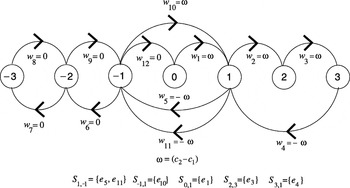
for epochs t1,…,tN. Let G = (V,E) be the directed graph induced by this sequence, where the vertex set V is obtained from {τk} (τk takes values in

) and the directed edge set E = {ek = (τk,τk+1)}. In the following, our discussion will be based on a graph so obtained from a sample path. For every ek ∈ E, define lk := τk+1 − τk and

. We will call lk the length of ek and call wk its weight. wk is the excess revenue earned by

over

due to the event at time tk. Also, define Sm,n := {ek ∈ E|τk = m,τk+1 = n}; that is, Sm,n is the set of all directed edges from

. Figure 5 shows an example of the directed graph induced by the τk from a sample path of the

systems.

Example sequence of τk from a sample path represented as a directed graph. For clarity in the illustration, self loops are not shown, as these do not have negative weights. The remaining edges are renumbered such that their initial order is maintained. In the example shown, m = 1 and m = 3 have edges with negative weights. Observe that the terms in (25) corresponding to these states are “canceled” as follows: [sum ]ek∈S1,−1 wk + [sum ]ek∈S−1,1 wk + [sum ]ek∈S1,0 wk = 0 and [sum ]ek∈S3,1 wk + [sum ]ek∈S2,3 wk = 0.
Now, consider the possible combination of events in

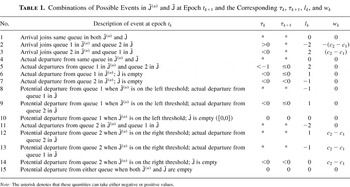
at epoch tk. They are listed in Table 1 along with the sign of τk and τk+1 and the values of lk and wk. From Table 1, we see that lk ∈ {−2,−1,0,1,2}, wk is negative only due to events of type 2 (an arrival chooses queue 1 in

and queue 2 in

), and if wk is negative, then τk > 0 and lk = −2. Further, lk > 0 and τk+1 > 0 are possible only from two events, those of type 3 and 12. A type 3 event is an arrival joining queue 2 in

and queue 1 in

. A type 12 event is a potential departure from queue 2 when

is on the right threshold and is, hence, disallowed and an actual departure from queue 2 in

. In this case, wk = c2 − c1 and lk = 1. We are now ready to state the following theorem.
Combinations of Possible Events in at Epoch tk+1 and the Corresponding τk, τk+1, lk, and wk

Theorem 8: If

start empty at time t = 0, then for all N ≥ 0,

Proof: We can write

We will use the sample-path graph G obtained as described earlier. To prove the theorem, we show that those Sm,n containing ek for which wk = (c1 − c2) < 0 are offset by edges with wk > 0 in (25). From Table 1, these sets will be of the form Sm,m−2, with m > 0. Consider one such vertex, say m, and let there be r edges, {ek1,ek2,…,ekr}, from m to m − 2 with negative weights. This means that [sum ]ek∈Sm,m−2 wk ≥ r(c1 − c2). Without loss of generality, we can assume that k1 < k2 < ··· < kr. Consider the two possibilities that arise.
Case 1: m = 1. Observe that τ1 = 0 and τk1 = 1. This guarantees that there must be a right-directed edge ek, an edge ek with lk > 0, with 0 < k < k1 into vertex 1. Now, consider the edge ekl from 1 to −1 with l > 1. Since τkl+1 = −1 and τkl+1 = 1, there must be a right-directed edge ek into vertex 1 with kl < k < kl+1. The right-directed edges obtained above are due to transitions at different time epochs and, hence, are distinct. This shows the existence of at least r right-directed edges into vertex 1. There are two types of right-directed edge into vertex 1, edges due to events of types 3 and 12, each of which have wk = c2 − c1. See Table 1. Thus,

Case 2: m > 1. Arguing as in Case 1, we can show that there are r right-directed edges into vertex m. The only possible right-directed edges into vertex m,m > 1, is due to an event of type 12. So, [sum ]ek∈Sm−1,m wk ≥ r(c2 − c1) and

See Figure 5 for an illustration of both cases.
For both of the cases, (25) can be written uniquely split into sums as in (26) and (27) and the theorem follows. █
The stationary revenue rate

defined in (17) becomes, by the Law of Large Numbers,
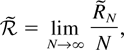
and from Theorems 7 and 8, we can now state the following theorem.
Theorem 9: If systems

start empty at t = 0, we have

5. NUMERICAL EXAMPLES AND DISCUSSION
The primary motivation for the truncation method that we adopted was to allow us to numerically calculate the performance parameters for the

systems, which, in turn, allows us to obtain the bounds for the

and the

systems. As has been described in van Houtum et al. [21], the truncated model is a quasi-birth–death (QBD) process. The necessary and sufficient conditions for the stability of the truncated systems can be numerically computed from Theorem 3.1.1 of Neuts [14]. Further, by a proper choice of the thresholds, the bounds can be made fairly tight. The steady state distribution of the truncated system can be calculated using the method described in Theorem 3.1.1 of [14].
We present numerical results to show the tightness of the bounds. For the non-work-conserving system, we consider λ1 = λ2 = 0.2 and μ1 = μ2 = 0.5, a1 = 0.8, a2 = 0.3, Tl = 0, and Tr = [lceil ][(1 − a2)/a2](c2 − c1)[rceil ] + 2. We compute the steady state distributions πx(u) and πx(l) and obtain the revenue rates

using (16). We also perform long-run simulations to obtain the steady state distribution πx and

for the

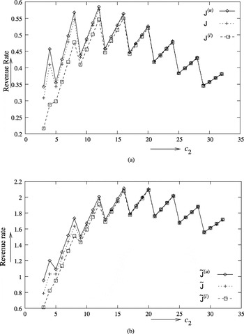
system. Figure 6a shows

as a function of c2, the join price of the costly queue, with c1 = 0. Similarly, for the work-conserving system, we plot

as a function of c2 for λ1 = λ2 = 0.4. μ1 = μ2 = 0.5, a1 = 0.8, a2 = 0.3, Tl = 0, and Tr = [lceil ][(1 − a2)/a2](c2 − c1)[rceil ] + 2 in Figure 6b. Observe that the bounds are very good for both the work-conserving and non-work-conserving systems, especially for c2 in the medium and high ranges.

Bounds on the revenue rates for the PMP and the Tirupati systems compared with results from a simulation model. (a) Revenue rates for the systems for different values of c2 with c1 = 0, λ1 = λ2 = 0.2, μ1 = μ2 = 0.5, a1 = 0.8, and a2 = 0.3. (b) Revenue rates for the systems for different values of c2 with c1 = 0, λ1 = λ2 = 0.4, μ1 = μ2 = 0.5, a1 = 0.8, and a2 = 0.3.
An important observation is that the revenue is not an increasing or a convex function of the prices.
6. EXTENSIONS AND CONCLUSION
We now discuss some possible extensions of the results in the previous sections to K,J > 2. Consider the queue join process for an arriving customer of an arbitrary class, say class α. For any two queues i and j, the surface xj − xi = [(1 − aα)/aα](ci − cj) decides the preference among the queues i and j for class α customers; that is, if the state is on the “right” of this surface, then the cost of joining queue j is less than that of joining queue i, otherwise the cost for i is lower. For any two queues, there exists such a surface and it will be denoted by

, where i and j are the queues and α is the customer class. For any customer class, only K − 1 of

are independent in the sense that they determine the remaining one.

will be the outermost K − 1 surfaces and these will, in turn, determine the other surfaces. Also, all of these surfaces will be concurrent on a line given by

This set of surfaces will together be called the attractors for customer class α. For J customer classes there will be J such parallel systems of surfaces. We first consider generalizing the stability results of Section 3 for J,K > 2.
6.1. Stability
First, consider the work-conserving system. The aggregated process

defined earlier is a birth–death process. Arguing as earlier, it is stable if and only if

and transient if and only if

. For the non-work-conserving JMCQ, the proof will require us to consider many cases and we conjecture that a similar result can be proved using quadratic Lyapunov functions.
6.2. Performance Bounds
As in Section 4.1, for a K-queue non-work-conserving JMCQ system, we consider the uniformized jump chain {xn}n≥0. The revenue rate is given by
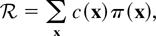
where c(x) is
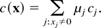
We can verify that the entire state space has a precedence property; the state

precedes state m + ei for i = 1,…,K, where, as previously, ei is a vector with 1 in the ith coordinate and 0 elsewhere. We use a truncated state space to obtain computable bounds for the revenue rate and other performance measures. The truncated state space

is the set of all x(t) = [x1,…,xK] such that Til ≤ xi − xK ≤ Tir for i = 1,2,…,K − 1 and Til ≤ minj∈{1,2,…,j}[(1 − aj)/aj](cK − ci) and Tir ≥ maxj∈{1,2,…,j}[(1 − aj)/aj](cK − ci). Let

be the surface xi − xK = Til and let

be the surface xi − xK = Tir. These are the “left” truncation surfaces and the “right” truncation surfaces, respectively. The upper and lower bounding systems like

, are defined over this truncated state space as earlier; departures that cause the system to leave the

are disallowed in

, whereas in

, they cause an additional simultaneous departure from queue K. By Theorem 1 of [21],

can be bounded by the revenue rates of

systems. We can also verify that the functions that capture the number in the system have the precedence property and, hence, we can find upper and lower bounds for the mean number in each queue.
The proof technique of obtaining performance bounds for the work-conserving JMCQ of Section 4.3 critically uses the fact that the state space is

. We believe that this methodology might not extend to models with more than two servers in a straightforward manner.
In conclusion, we have presented a generalization of the JSQ queuing system by allowing queues to prescribe join costs and customers to define cost functions in terms of the queue lengths seen on arrival and the join price. The stability results are discussed. We have also presented a technique to define truncated systems that will bound the original systems from above and below and are amenable to numerical calculations of the relevant performance measures using matrix geometric techniques developed for quasi-birth–death processes.
Acknowledgment
We thank the referee for very useful suggestions that helped in completely characterizing the stability conditions and also in the simplification of the proofs of our results on the non-work-conserving JMCQ.
References
REFERENCES
Asmussen, S.
(1987).
Applied probability and queues.
Chichester:
Wiley.
Blake, S.,
Black, D.,
Carlson, M.,
Davies, E.,
Wang, Z., &
Weiss, W.
(1998).
An architecture for differentiated services.
Internet Engineering Task Force, Request for Comments #2475,
Dec. 1998
(ftp://ftp.isi.edu/in-notes/rfc2475.txt).
Borkar, V.S. &
Manjunath, D.
(2002).
Charge based control of DiffServ queues,
submitted.
Boxma, O.,
Koole, G., &
Liu, Z.
(1996).
Queueing theoretic solution methods for models of parallel and
distributed systems. In
O. Boxma &
G. Koole (eds.),
Performance evaluation of parallel and distributed
systems—Solution methods,
CWI Tract No. 105.
Amsterdam, pp.
1–24.
Bremaud, P.
(1998).
Markov chains, Gibbs fields, Monte Carlo simulation, and queues.
New York:
Springer-Verlag.
Dube, P.,
Borkar, V.S., &
Manjunath, D.
(2002).
Differential join prices for parallel queues: Social optimality,
dynamic pricing algorithms and application to Internet pricing. In
Proceedings of IEEE INFOCOM 2002.
Falkner, M.,
Devetsikiotis, M., &
Lambadaris, I.
(2000).
An overview of pricing concepts for broadband IP networks.
IEEE Communications Surveys
3:
2–13.Google Scholar
Foley, R.D. &
McDonald, D.R.
(2001).
Join the shortest queue: Stability and exact asymptotics.
Annals of Applied Probability
11(3):
569–607.Google Scholar
Gibbens, R.,
Mason, R., &
Steinberg, R.
(2000).
Internet service classes under competition.
IEEE Journal on Selected Areas in Communications
18(12):
2490–2498.Google Scholar
Jain, R.,
Mullen, R., &
Hausman, R.
(2001).
Analysis of Paris Metro pricing strategy for QoS with a single
service provider. In
Proceedings of the Ninth International Workshop on Quality of
Service (IWQoS 2001).
Kingman, J.F.C.
(1962).
Two queues in parallel.
Annals of Mathematical Statistics
32:
1314–1323.Google Scholar
Manjunath, D.,
Goel, A., &
Hemachandra, N.
(2002).
DiffServ node with join minimum cost queue policy: Analysis with
multiclass traffic. In
Proceedings of IEEE Globecom 2002
3:
2573–2577.Google Scholar
Mertens, J.F.,
Samuel-Cahn, E., &
Zamir, S.
(1978).
Necessary and sufficient conditions for recurrence and transience
of Markov chains, in terms of inequalities.
Journal of Applied Probability
15:
848–851.Google Scholar
Neuts, M.F.
(1981).
Matrix geometric solutions in stochastic models.
Baltimore:
Johns Hopkins University Press.
Norris, J.R.
(1999).
Markov chains.
Cambridge:
Cambridge University Press.
Odlyzko, A.
(1999).
Paris Metro pricing for the Internet. In
Proceedings of the ACM Conference on Electronic Commerce, pp.
140–147.
Parekh, A.K. &
Gallager, R.G.
(1993).
A generalized processor sharing approach to flow control in
integrated services networks: The single node case.
IEEE/ACM Transactions on Networking
1(3):
344–357.Google Scholar
Serfozo, R.
(1999).
Introduction to stochastic networks.
New York:
Springer-Verlag.
Tandra, R.,
Hemachandra, N., &
Manjunath, D.
(2004).
DiffServ node with join minimum cost queue policy and multiclass
traffic.
Performance Evaluation
55:
69–91.Google Scholar
van Houtum, G.J.,
Zijm, W.H.M.,
Adan, I.J.B.F., &
Wessels, J.
(1998).
Bounds for performance characteristics: A systematic approach via
cost structures.
Stochastic models
14:
205–224.Google Scholar
van Houtum, G.J.,
Adan, I.J.B.F.,
Wessels, J., &
Zijm, W.H.M.
(2000).
Performance analysis of parallel identical machines with a
generalized shortest queue arrival mechanism,
OR Spektrum
23:
411–428.Google Scholar
Walrand, J.
(1988).
Introduction to queueing networks.
Englewood Cliffs, NJ:
Prentice-Hall.
Wolff, R.
(1989).
Stochastic modeling and the theory of queues.
Englewood Cliffs, NJ:
Prentice-Hall.
Plots illustrating the differentiated service provided by JMCQ. (a) Mean waiting time of customers of different classes for the work-conserving JMCQ system compared with that of the JSQ system. (b) Mean queue lengths for the work-conserving JMCQ compared with the mean queue length in the JSQ system.
The transition rates for {x(t)}t≥0, the CTMC for the non-work-conserving queue system. Partitions A1,…,A5 and F used in the stability analysis of Theorem 1 are also shown.
The transition rates for , the CTMC for the evolution of the work-conserving JMCQ. Observe that the departure rates for states on the axes are μ = μ1 + μ2.
The truncated state space for the systems. The modified transitions rates for states on are shown. The transition rates for the states between the truncation lines are the same as that of system shown in Figure 2. (a) Transition rates for the system. For states in , transitions due to departures from queue 1 (2) are disallowed. (b) Transition rates for the system. For states , there is a diagonal transition with a rate μ1 (μ2).
Example sequence of τk from a sample path represented as a directed graph. For clarity in the illustration, self loops are not shown, as these do not have negative weights. The remaining edges are renumbered such that their initial order is maintained. In the example shown, m = 1 and m = 3 have edges with negative weights. Observe that the terms in (25) corresponding to these states are “canceled” as follows: [sum ]ek∈S1,−1 wk + [sum ]ek∈S−1,1 wk + [sum ]ek∈S1,0 wk = 0 and [sum ]ek∈S3,1 wk + [sum ]ek∈S2,3 wk = 0.
Combinations of Possible Events in at Epoch tk+1 and the Corresponding τk, τk+1, lk, and wk
Bounds on the revenue rates for the PMP and the Tirupati systems compared with results from a simulation model. (a) Revenue rates for the systems for different values of c2 with c1 = 0, λ1 = λ2 = 0.2, μ1 = μ2 = 0.5, a1 = 0.8, and a2 = 0.3. (b) Revenue rates for the systems for different values of c2 with c1 = 0, λ1 = λ2 = 0.4, μ1 = μ2 = 0.5, a1 = 0.8, and a2 = 0.3.
 You have
Access
- 8
- Cited by