





1. Introduction
The present work explores the vibrations emerging when an elastically mounted circular cylinder placed in quiescent fluid is subjected to a forced rotation about its axis. Beyond its possible implications for applications (e.g. mixing), this problem may be regarded as a paradigm to study the interaction phenomena appearing in quiescent fluid due to an actuation of the body.
The impact of a forced rotation on the fluid–body system behaviour has been well documented for a cylinder exposed to a cross-current, and thus susceptible to vortex-induced vibrations (VIV) (Stansby & Rainey Reference Stansby and Rainey2001; Yogeswaran & Mittal Reference Yogeswaran and Mittal2011; Bourguet & Lo Jacono Reference Bourguet and Lo Jacono2014; Zhao et al. Reference Zhao, Cheng and Lu2014; Seyed-Aghazadeh & Modarres-Sadeghi Reference Seyed-Aghazadeh and Modarres-Sadeghi2015; Wong et al. Reference Wong, Zhao, Lo Jacono, Thompson and Sheridan2017; Bourguet Reference Bourguet2020, Reference Bourguet2023; Munir et al. Reference Munir, Zhao, Wu and Tong2021; Zhao et al. Reference Zhao, Thompson and Hourigan2022; Lu et al. Reference Lu, Zhang and Zhang2025). VIV are a form of flow-induced vibrations driven by a synchronisation of body motion and flow unsteadiness associated with vortex formation in the wake (Williamson & Govardhan Reference Williamson and Govardhan2004). Without rotation, VIV exhibit peak amplitudes of the order of one body diameter in the cross-flow direction, and one or more orders of magnitude lower in the streamwise direction. The rotation breaks the transverse symmetry of the system behaviour, enhances cylinder oscillations and may trigger a transition from VIV to another form of structural responses, referred to as galloping-like, whose magnitude increases unboundedly with the reduced velocity (inverse of the oscillator natural frequency, non-dimensionalised by the body diameter and the current velocity).
A forced rotation of the cylinder can induce vibrations in the absence of cross-current, i.e. in quiescent fluid. Such rotation-induced vibrations (RIV) were first detected for a cylinder free to translate along a rectilinear path, without structural restoring force (Bourguet Reference Bourguet2025a
). In this configuration, the system behaviour is aperiodic and the irregular oscillations of the body may exceed ten diameters. When the rotating cylinder is attached to an elastic support, rectilinear RIV may also develop through periodic regimes, whose responses differ by their spectral contents, sinusoidal versus multi-harmonic, in addition to the aperiodic regime identified without structural restoring force (Bourguet Reference Bourguet2025b
). RIV occur over broad ranges of the governing parameters, i.e. the Reynolds number (Re) and the reduced velocity (
 $U^\star$
), both based on the surface velocity of the rotating body and its diameter, the structure to displaced fluid mass ratio (
 $m^\star$
), and the structural damping ratio (
 $\xi$
). More precisely, RIV were encountered from
 $\textit{Re}\approx 4$
up to the largest value considered in this prior work,
 $\textit{Re}=100$
, over several orders of magnitude of
 $m^\star$
, and for substantially damped oscillators. The large amplitudes attained in the high-
 $U^\star$
range are reminiscent of the galloping-like responses observed for a rotating cylinder immersed in a cross-current. This trend suggests that the rectilinear RIV could be driven by a quasi-steady mechanism, where the time scales of the flow and moving cylinder are decoupled, like the oscillations of non-axisymmetric bodies (Modarres-Sadeghi Reference Modarres-Sadeghi2022). It appears that this is not the case: the vibrations are not captured by a quasi-steady modelling of fluid forcing, i.e. based on the time-averaged forces measured when the body is rigidly mounted within a steady current. This substantiates the role of the interplay of the cylinder with flow unsteadiness in the development of RIV. In addition, the interaction of the cylinder with previously shed vortices, which are not convected away in the absence of current, may explain the emergence of irregular dynamics, as also reported in oscillatory flow studies (e.g. Anagnostopoulos & Iliadis Reference Anagnostopoulos and Iliadis1998; Dorogi et al. Reference Dorogi, Baranyi and Konstantinidis2023).
At this step, the exploration of RIV is limited to a single-degree-of-freedom oscillator, where the cylinder is restrained to move along a rectilinear path. Allowing the body to translate in the plane normal to its axis, by adding a second degree of freedom, may considerably alter the system behaviour. Such alteration was illustrated, for example, in prior studies concerning VIV, where novel response branches and flow patterns arose after the introduction of a second degree of freedom (Jauvtis & Williamson Reference Jauvtis and Williamson2004; Gsell et al. Reference Gsell, Bourguet and Braza2019). The object of the present work is to investigate the RIV occurring in the plane, for a two-degree-of-freedom oscillator. Some insights can be gained from the analysis proposed by Stansby & Rainey (Reference Stansby and Rainey2001), initially developed for a rotating cylinder in a cross-current, but also applicable to the quiescent fluid configuration. Based on the balance of radial forces, thus taking into account the Magnus effect (Prandtl Reference Prandtl1926), and potential flow assumption, this analysis identified two forms of periodic solutions characterised by circular orbits of the cylinder. These circular orbits are oriented either in the same sense as the forced rotation with a frequency larger than the natural frequency of the oscillator or in the opposite sense with a frequency lower than the natural frequency. For large ratios between the cylinder surface velocity and the oncoming flow velocity, i.e. in the cases closest to the present quiescent fluid configuration, the latter form of responses actually dominates simulation and experimental results, as also noted in subsequent studies (Yogeswaran & Mittal Reference Yogeswaran and Mittal2011; Bourguet Reference Bourguet2020, Reference Bourguet2023). The possible coexistence of these two forms of structural responses, and the appearance of less regular dynamics, remain to be clarified for a rotating cylinder in quiescent fluid. Another aspect that needs to be studied is the validity of a quasi-steady approach to predict the two-degree-of-freedom RIV. In contrast to the rectilinear oscillations where the body permanently collides with previously formed vortices, such modelling of fluid forcing could become reasonable, at least for circular trajectories of sufficiently large radii. Under a quasi-steady assumption, the cancellation and possibly negative values of the drag force, due to the imposed rotation (Stojković et al. Reference Stojković, Breuer and Durst2002), suggest that stable orbits could be reached, including for damped oscillators. These different aspects will be addressed in the paper.
To present a global vision of the two-degree-of-freedom RIV, the behaviour of the system composed of an elastically mounted circular cylinder, subjected to a forced rotation and free to move in both directions normal to its axis, in quiescent fluid, is investigated over ranges of the four governing parameters, Re and
 $U^\star$
up to
 $100$
and
 $200$
, respectively,
 $m^\star \in [1,100]$
and
 $\xi$
up to
 $50\,\%$
. The parameter space is comparable to that considered in the above-mentioned study concerning rectilinear RIV (Bourguet Reference Bourguet2025b
). It is covered by numerical simulations involving the coupled, unsteady flow-body system equations, referred to as ‘unsteady simulations’ in the following, as opposed to the quasi-steady approach, which is also employed to shed light on the underlying physical mechanisms and to predict some general trends.
The paper is organised as follows. The physical system and the numerical method are described in § 2. A quasi-steady analysis of the problem is presented in § 3. The validity of the quasi-steady approach is assessed in § 4, where the system behaviour is examined based on the unsteady simulation results. The principal findings of this work are summarised in § 5.
2. Formulation and numerical method
The fluid–body system, its modelling and the parameter space under study are described in § 2.1. The numerical method employed is presented in § 2.2.
2.1. Physical system
The physical system is schematised in figure 1. The configuration is the same as in the previous study concerning a rotating circular cylinder, elastically mounted in quiescent fluid (Bourguet Reference Bourguet2025b ), except that in the present work, the body is free to move in both directions normal to its axis, instead of a single direction.
Sketch of the physical system.

The
 $(x,y,z)$
frame is fixed. The cylinder of diameter
 $D$
and mass per unit length
 $M_c$
is parallel to the
 $z$
axis. It is mounted on elastic supports of structural stiffness per unit length
 $k$
and damping per unit length
 $d$
. The body is free to translate along the
 $x$
and
 $y$
axes within a quiescent fluid of density
 $\rho _{\!f}$
and viscosity
 $\mu$
. The cylinder is subjected to a forced, counter-clockwise, steady rotation of angular velocity
 $\varOmega$
, about its axis. All the physical variables are non-dimensionalised by
 $\rho _{\!f}$
,
 $D$
and the cylinder surface velocity
 $U=\varOmega D/2$
. The cylinder displacements in the
 $x$
and
 $y$
directions, non-dimensionalised by
 $D$
, are denoted by
 $\zeta _x$
and
 $\zeta _{\!y}$
, respectively. The force coefficients are defined as
 $C_x=2F_x/(\rho _{\!f} D U^2)$
and
 $C_{\!y}=2F_{\!y}/(\rho _{\!f} D U^2)$
, where
 $F_x$
and
 $F_{\!y}$
are the dimensional fluid forces per unit length aligned with the
 $x$
and
 $y$
axes, respectively.
The dynamics of the two-degree-of-freedom oscillator is governed by the following equations:
 \begin{align} \ddot {\zeta }_x + \dfrac {4\pi \xi }{U^\star }\dot {\zeta }_x + \left (\dfrac {2\pi }{U^\star }\right )^2 \zeta _x = \dfrac {2 C_x}{\pi m^\star }, \\[-12pt]\nonumber \end{align}
 \begin{align} \ddot {\zeta }_{\!y} + \dfrac {4\pi \xi }{U^\star }\dot {\zeta }_{\!y} + \left (\dfrac {2\pi }{U^\star }\right )^2 \zeta _{\!y} = \dfrac {2 C_{\!y}}{\pi m^\star }, \end{align}
where the dot
 $\dot {\phantom {a}}$
designates the non-dimensional time derivative. The structure to displaced fluid mass ratio, structural damping ratio, non-dimensional natural frequency and associated reduced velocity are defined as
 $m^\star =4 M_c/(\pi \rho _{\!f} D^2)$
,
 $\xi =d/(2\sqrt {k M_c})$
,
 $f_n=[D/(2\pi U)]\sqrt {k/M_c}$
and
 $U^\star =1/f_n$
, respectively.
The mass ratio is varied from
 $1$
to
 $100$
and the reduced velocity up to
 $200$
. Structural damping is introduced in specified cases and set to zero otherwise. The Reynolds number,
 $\textit{Re}=\rho _{\!f} U D/\mu$
, is kept below or equal to
 $100$
. This choice ensures that the flow remains two-dimensional over most of the parameter space. As also noted in the above-mentioned study concerning rectilinear RIV, the three-dimensional transition may occur in the higher-Re range, typically beyond
 $\textit{Re}=75$
. The transition is not examined in the present paper and the two-dimensional Navier–Stokes equations are employed throughout the parameter space to predict the flow dynamics. Yet, additional three-dimensional simulations indicate that the main features of the system behaviour described hereafter, in particular, the distinct regimes through which RIV develop, persist beyond the transition.
Each unsteady simulation is initialised with the established flow past a rigidly mounted, rotating cylinder. Then, the body is released with an initial displacement, to break the axial symmetry. The amplitude of this initial displacement is discussed in the following. Previous studies on cylinder VIV have identified hysteresis phenomena, where the permanent behaviour reached by the system after the transient dies out depends on the initial condition (e.g. Khalak & Williamson Reference Khalak and Williamson1999; Prasanth et al. Reference Prasanth, Premchandran and Mittal2011). To explore the different solutions that may coexist in each point of the parameter space, two initial conditions are employed here: a small initial displacement
 $(\zeta _x(0),\zeta _{\!y}(0))=(0.05,0)$
(condition A) and a large initial displacement (condition B). In the latter condition, the initial displacement corresponds to the largest displacement predicted by the quasi-steady approach described in § 3. No other solution branches than those captured after an initialisation with condition A or B have been detected by considering more initial conditions, including intermediate and larger magnitudes of the initial displacement; this point is illustrated in an Appendix dedicated to the influence of the initial condition.
A series of additional simulations, where the rotating cylinder is rigidly mounted within a cross-current, is also carried out over the Re range under study to measure the force coefficients used in the quasi-steady analysis.
2.2. Numerical method
The numerical method is the same as in previous studies concerning comparable systems (Bourguet & Lo Jacono Reference Bourguet and Lo Jacono2014; Bourguet Reference Bourguet2020, Reference Bourguet2023, Reference Bourguet2025a , Reference Bourguetb ). Descriptions of the simulation approach, as well as detailed validations, were reported in these prior works. The method is briefly summarised here and some additional convergence results are presented.
The coupled flow–structure equations are solved by the parallelised code Nektar, which is based on the spectral/hp element method (Karniadakis & Sherwin Reference Karniadakis and Sherwin1999). Body motion is taken into account by adding inertial terms in the Navier–Stokes equations (Newman & Karniadakis Reference Newman and Karniadakis1997). The cylinder is placed at the centre of a large square computational domain of side length
 $600D$
. The size of the domain avoids any spurious blockage effects. The computational domain is discretised into
 $3975$
spectral elements. A no-slip condition is applied on the cylinder surface and a Neumann-type boundary condition is used on the external boundaries.
Unsigned relative differences of the (a) maximum value and (b) dominant frequency of
 $\zeta _x$
for
 $(\textit{Re},m^\star ,U^\star )=(100,10,60)$
, with respect to the reference results obtained for a polynomial order
 $N_{\!p}=5$
and a non-dimensional time step
 $\Delta t=0.0025$
, as functions of
 $N_{\!p}$
and
 $\Delta t$
. The values of the unsigned relative differences are specified in the plots. The reference set of parameters is denoted by the symbol
 $R$
and the selected set by a star.

A convergence study in a typical case where the rotating cylinder vibrates at the largest Re value considered in this work (Re
 $\,=100$
) is depicted in figure 2. The unsigned relative differences of the maximum value of
 $\zeta _x$
signal and its dominant frequency (
 $f_\zeta$
), with respect to the results obtained for a polynomial order
 $N_{\!p}=5$
and a non-dimensional time step
 $\Delta t=0.0025$
, are represented as functions of
 $N_{\!p}$
and
 $\Delta t$
. An increase from
 $N_{\!p}=4$
to
 $N_{\!p}=5$
and a reduction from
 $\Delta t=0.005$
to
 $\Delta t=0.0025$
have no impact on the results. A polynomial order of
 $4$
and a time step of
 $0.005$
were selected, as in the previous study on rectilinear RIV (Bourguet Reference Bourguet2025b
).
Validation results in physical configurations close to the present one were reported in the above-mentioned study on rectilinear RIV. These results include comparisons with prior simulations concerning a non-rotating cylinder, either forced to oscillate in quiescent fluid (Elston et al. Reference Elston, Blackburn and Sheridan2006; Koehler et al. Reference Koehler, Beran, Vanella and Balaras2015) or elastically mounted in the direction normal to an oscillatory flow (Dorogi et al. Reference Dorogi, Baranyi and Konstantinidis2023). These validation studies complemented those proposed in the papers listed at the beginning of this subsection, where rotating and non-rotating cylinders were exposed to cross-currents.
The investigation of the system behaviour presented hereafter is based on time series collected after the initial transient dies out, over sufficiently long periods to ensure convergence of body dynamics and fluid force statistics.
3. Quasi-steady analysis
To shed some light on the underlying physical mechanisms, a quasi-steady analysis of the problem is proposed in this section. The analysis relies on a decoupling of body motion and flow unsteadiness time scales. The modelling of fluid forces based on such a decoupling is explained in § 3.1. When this modelling of the forces is introduced in the dynamics equations (2.1), specific forms of responses, characterised by circular trajectories, can be identified. These responses are examined in § 3.2. In addition to these circular orbits, another form of responses is predicted by the proposed modelling approach. It is described in § 3.3 and a quasi-steady vision of the system behaviour, across the parameter space, is presented.
Sketches of the (a) instantaneous flow seen by the cylinder moving in quiescent fluid, (b) rigidly mounted body configuration considered in the quasi-steady approach and (c) quasi-steady modelling of fluid forces. In the rigidly mounted body configuration, the magnitude of the steady cross-current velocity matches the velocity magnitude of the instantaneous flow seen by the moving cylinder (
 $V$
).

Time-averaged coefficients of the forces (a) parallel and (b) normal to the oncoming flow, for a rigidly mounted rotating cylinder placed in a steady cross-current, as functions of the Reynolds number and the magnitude of the current velocity. The iso-contour
 $\overline {C_{\scriptscriptstyle \parallel }}=0$
, which delimits the region where the drag force exerted on the body becomes a thrust force, i.e.
 $\overline {C_{\scriptscriptstyle \parallel }}\lt 0$
, is represented by a dashed line. The section of this iso-contour associated with a negative/positive gradient of
 $\overline {C_{\scriptscriptstyle \parallel }}$
with respect to
 $V$
, is coloured in black/white.

3.1. Fluid force modelling
At each step of the motion, the quasi-steady approach consists in modelling the fluid forces via the time-averaged forces measured when the cylinder is rigidly mounted within a steady cross-current, whose velocity matches the instantaneous velocity seen by the moving body (e.g. Parkinson & Smith Reference Parkinson and Smith1964). The instantaneous velocity seen by the moving body, schematised in figure 3(a), is
 $\{-\dot \zeta _x,-\dot \zeta _{\!y},0\}^T$
. Its magnitude is
 $V=\sqrt {\dot \zeta ^2_x+\dot \zeta ^2_{\!y}}$
and its incidence angle relative to the
 $x$
axis,
 $\beta$
, satisfies
 $\tan (\beta )=(-\dot \zeta _{\!y})/(-\dot \zeta _x)$
. In the rigidly mounted body configuration, the coefficients of the forces parallel and normal to the steady cross-current of velocity magnitude
 $V$
are denoted by
 $C_{\scriptscriptstyle \parallel }$
and
 $C_\perp$
, respectively (figure 3
b). Force normalisation is the same as for
 $C_x$
and
 $C_{\!y}$
, i.e. based on the surface velocity
 $U$
. Within the quasi-steady framework, the time-averaged coefficients
 $\overline {C_{\scriptscriptstyle \parallel }}$
and
 $\overline {C_\perp }$
represent the forces aligned with and normal to the instantaneous velocity of the flow seen by the moving cylinder (figure 3
c). The overline symbol
 $\overline {\phantom {a}}$
denotes the time-averaged values. It should be mentioned that throughout the parameter space investigated, the Reynolds number based on
 $V$
(
 $\textit{Re}V$
), and the ratio between the cylinder surface velocity and
 $V$
(rotation rate,
 $1/V$
), correspond to conditions where the flow past a rigidly mounted cylinder is steady and, therefore,
 $\overline {C_{\scriptscriptstyle \parallel }}=C_{\scriptscriptstyle \parallel }$
and
 $\overline {C_\perp }=C_\perp$
. Yet, to keep some generality in the presentation, the overline symbol is still used in the following.
The evolutions of
 $\overline {C_{\scriptscriptstyle \parallel }}$
and
 $\overline {C_\perp }$
in the
 $(\textit{Re},V)$
domain are plotted in figure 4. Beyond
 $\textit{Re}\approx 7$
,
 $\overline {C_{\scriptscriptstyle \parallel }}$
is found to become negative over a range of
 $V$
values, i.e. the drag force exerted on the body becomes a thrust force (figure 4
a). The region where
 $\overline {C_{\scriptscriptstyle \parallel }}\lt 0$
is delimited by a dashed line. Within this region, as shown in § 3.2, the thrust induced by the imposed rotation can counterbalance the effect of structural damping and result in a sustained motion of the body. Assuming that a value of
 $\overline {C_{\scriptscriptstyle \parallel }}$
corresponds to an equilibrium state of the system, for example
 $\overline {C_{\scriptscriptstyle \parallel }}=0$
for a body moving at a constant velocity without damping, as discussed hereafter, then a slight departure from the associated value of
 $V$
tends to be amplified or attenuated by fluid forcing, depending on the sign of the force gradient with respect to
 $V$
. A negative gradient of
 $\overline {C_{\scriptscriptstyle \parallel }}$
corresponds to an unstable equilibrium, while a positive gradient corresponds to a stable equilibrium. In figure 4, the unstable and stable equilibria along the
 $\overline {C_{\scriptscriptstyle \parallel }}=0$
iso-contour (dashed line) are represented in black and white, respectively. The normal force associated with the Magnus effect is negative due to the counter-clockwise orientation of the imposed rotation. As shown in figure 4(b),
 $\overline {C_\perp }$
exhibits a monotonically decreasing evolution as a function of
 $V$
.
The quasi-steady models of the force coefficients
 $C_x$
and
 $C_{\!y}$
, identified by the superscript
 ${}^{qs}$
, are obtained via the projections of
 $\overline {C_{\scriptscriptstyle \parallel }}$
and
 $\overline {C_\perp }$
onto the
 $x$
and
 $y$
axes:
 \begin{align} C^{qs}_x =\overline {C_{\scriptscriptstyle \parallel }}\left (V\right )\cos \left (\beta \right )-\overline {C_\perp }\left (V\right )\sin \left (\beta \right )\!, \\[-12pt]\nonumber \end{align}
 \begin{align} C^{qs}_{\!y} =\overline {C_{\scriptscriptstyle \parallel }}\left (V\right )\sin \left (\beta \right )+\overline {C_\perp }\left (V\right )\cos \left (\beta \right )\!. \end{align}
A schematic view of
 $C^{qs}_x$
and
 $C^{qs}_{\!y}$
, and of their link to
 $\overline {C_{\scriptscriptstyle \parallel }}$
and
 $\overline {C_\perp }$
, is presented in figure 3(c). In the following, the quasi-steady models of the force coefficients (
 $C^{qs}_x$
and
 $C^{qs}_{\!y}$
) are introduced in the dynamics equations (2.1) to predict the system behaviour.
3.2. Circular orbits
When the force coefficients (
 $C_x$
and
 $C_{\!y}$
) are replaced by their quasi-steady models (
 $C^{qs}_x$
and
 $C^{qs}_{\!y}$
) in the dynamics equations (2.1), specific forms of solutions characterised by circular trajectories can be identified, as explained hereafter.
As a first step, considering the displacements expressed in polar coordinates
 $(r,\theta )$
, such as
 $\zeta _x=r\cos (\theta )$
and
 $\zeta _{\!y}=r\sin (\theta )$
, the dynamics equations (2.1) are written as follows:
 \begin{align} \ddot {r} - r \dot \theta ^2 + \dfrac {4\pi \xi }{U^\star }\dot {r} + \left (\dfrac {2\pi }{U^\star }\right )^2 r = \dfrac {2 C_r}{\pi m^\star }, \\[-12pt]\nonumber \end{align}
 \begin{align} r\ddot {\theta } + 2 \dot {r} \dot \theta + \dfrac {4\pi \xi }{U^\star } r\dot {\theta } = \dfrac {2 C_\theta }{\pi m^\star }, \end{align}
where the radial and azimuthal force coefficients are
 \begin{equation} C_r =C_x\cos \left (\theta \right ) + C_{\!y}\sin \left (\theta \right )\quad\mathrm{and}\quad C_\theta =-C_x\sin \left (\theta \right ) + C_{\!y}\cos \left (\theta \right ). \end{equation}
The coordinate system change from Cartesian to polar coordinates is schematised in figure 5(a).
Sketches of the (a) coordinate system change from Cartesian to polar coordinates and (b) quasi-steady modelling of fluid forces along a circular trajectory, where the body moves with a positive or negative azimuthal velocity.

Then, introducing the quasi-steady approximation of fluid forces (3.1), it appears that a periodic, circular orbit where the cylinder moves at a constant velocity, i.e.
 $\dot {r}=\ddot {r}=\ddot \theta =0$
, can be a solution of the above-mentioned dynamics equations. In this case, the cylinder velocity along the circular trajectory (azimuthal velocity) is
 $U_\theta =r\dot \theta$
. The instantaneous velocity magnitude of the flow seen by the body and the force coefficients become
 \begin{equation} V=|U_\theta |,\,\,C^{qs}_r=\dfrac {U_\theta }{|U_\theta |}\overline {C_\perp }\left (|U_\theta |\right )\quad\mathrm{ and}\quad C^{qs}_\theta =-\dfrac {U_\theta }{|U_\theta |}\overline {C_{\scriptscriptstyle \parallel }}\left (|U_\theta |\right ), \end{equation}
as illustrated in figure 5(b). The dynamics equations (3.2) can be expressed as
 \begin{align} \dot \theta ^2+\dfrac {2\overline {C_\perp }\left (|U_\theta |\right )}{\pi m^\star |U_\theta |}\dot \theta -\left (\dfrac {2\pi }{U^\star }\right )^2=0, \\[-12pt]\nonumber \end{align}
 \begin{align} -\dfrac {2 \pi ^2 m^\star \xi }{U^\star }|U_\theta |=\overline {C_{\scriptscriptstyle \parallel }}\left (|U_\theta |\right )\!. \end{align}
The latter equation represents the balance between the damping and thrust forces mentioned in § 3.1. For given values of
 $m^\star$
and
 $U^\star$
, there exists a critical value of
 $\xi$
beyond which this equation cannot be satisfied by
 $|U_\theta |\gt 0$
. Beyond this threshold, the solutions characterised by circular orbits disappear.
Based on the dynamics equations (3.5), the circular orbit properties are derived as follows. Values of
 $|U_\theta |$
(equal to
 $V$
) that satisfy (3.5b
) are determined from the evolution of
 $\overline {C_{\scriptscriptstyle \parallel }}$
versus
 $V$
, depicted in figure 4(a). Due to the non-monotonic trend of
 $\overline {C_{\scriptscriptstyle \parallel }}$
, two positive values of
 $|U_\theta |$
are generally identified. The higher value, which is associated with a positive gradient of the force and thus to a stable equilibrium state, is expected to be selected by the system. This point will be confirmed in § 3.3. Once
 $|U_\theta |$
is known, the value of
 $\overline {C_\perp }$
is fixed (figure 4
b). Then, the second-order equation (3.5a
) can be solved to find the angular velocity
 $\dot \theta$
:
 \begin{equation} \dot \theta =\dfrac {\dot \theta _\infty }{2}\pm \sqrt {\left (\dfrac {\dot \theta _\infty }{2}\right )^2+\left (\dfrac {2\pi }{U^\star }\right )^2}\quad \mathrm{ with} \quad \dot \theta _\infty =-\dfrac {2\overline {C_\perp }\left (|U_\theta |\right )}{\pi m^\star |U_\theta |}. \end{equation}
The radius of the circular orbit and the revolution frequency are equal to
 $r=U_\theta /\dot \theta$
and
 $f_\zeta =|\dot \theta |/(2\pi )$
, respectively. The two solutions are oriented in opposite senses. For the positive
 $\dot \theta$
solution, where the body moves in the same sense as the imposed rotation, the revolution frequency is larger than
 $f_n$
, while for the negative
 $\dot \theta$
solution, where the body moves in the opposite sense,
 $f_\zeta$
is lower than
 $f_n$
. The radius of the circular orbit is larger for
 $\dot \theta \lt 0$
and tends to infinity with
 $U^\star$
, while it saturates and tends to
 $U_\theta /\dot \theta _\infty$
for
 $\dot \theta \gt 0$
.
The two forms of periodic solutions are named C
 $^+$
and C
 $^-$
in the following, in reference to the circular trajectory and its orientation, in the sense of the forced rotation (
 $+$
) or in the opposite sense (
 $-$
). The circular orbit solutions were previously detected by Stansby & Rainey (Reference Stansby and Rainey2001), based on the potential flow assumption. Here, the introduction of a quasi-steady modelling of fluid forces allows to determine the velocity magnitude (
 $|U_\theta |$
) compatible with force equilibrium in the azimuthal direction (equation (3.5b
)) and thus deduce the orbit radii. This is not feasible via the potential flow approach since the drag force always vanishes. The quasi-steady approximation of the radial force contribution is also expected to be more accurate than the potential flow estimate; in the latter approach,
 $\overline {C_\perp }/|U_\theta |$
is replaced by
 $-2\pi$
in (3.5a
).
Quasi-steady simulation results are presented in the next subsection to validate the above-mentioned analysis concerning the circular orbits and to investigate the emergence of other forms of responses.
3.3. Quasi-steady simulations
Quasi-steady simulations, where
 $C^{qs}_x$
and
 $C^{qs}_{\!y}$
(expressions (3.1)) are used instead of
 $C_x$
and
 $C_{\!y}$
in the dynamics equations (2.1), are carried out for
 $(\textit{Re},m^\star )=(50,10)$
and
 $U^\star \in \{40,70,100\}$
. The structural damping is set to zero (
 $\xi =0$
); its influence will be addressed later in the paper (§ 4.2.3). A range of initial conditions is considered to capture the different solutions. These solutions are visualised in figure 6, through body trajectories (panels a) and frequency spectra of the displacement along the
 $x$
axis (panels b). In the spectra, the displacement spectral amplitude is normalised by its maximum value and the frequency range by the natural frequency of the oscillator.
(a) Cylinder trajectories and (b) frequency spectra of the
 $x$
axis displacement issued from quasi-steady simulations, for
 $(\textit{Re},m^\star )=(50,10)$
and three values of the reduced velocity: (i)
 $U^\star =40$
, (ii)
 $U^\star =70$
and (iii)
 $U^\star =100$
. The three forms of responses (C
 $^+$
, C
 $^-$
and
 $M$
) are obtained by considering different initial conditions. The orientations of the trajectories are indicated by arrows in panel (aii). In panels (b), the response form is specified in each spectrum, the displacement spectral amplitude is normalised by its maximum value and the frequency range is scaled by the oscillator natural frequency; the frequency ratio of
 $1$
is denoted by a grey dashed line. In the last row of spectra (M responses), the harmonic frequencies of the low-frequency component are represented by red dotted lines and the high-frequency component is indicated by a red arrow.

Figure 6. Long description
The image contains six graphs divided into two rows. The top row (a) shows scatter plots of cylinder trajectories, while the bottom row (b) displays line graphs of frequency spectra. Each column represents different values of reduced velocity. Panel (ai) shows a small, circular trajectory with three lines labeled C+, C-, and M. Panel (aii) depicts a larger, elliptical trajectory with the same labels. Panel (aiii) illustrates an even larger, circular trajectory. The frequency spectra in panels (bi), (bii), and (biii) show spectral amplitude versus frequency ratio for the C+, C-, and M responses, respectively. Each spectrum is normalized by its maximum value, with the frequency range scaled by the oscillator natural frequency. The M responses include harmonic frequencies marked by red dotted lines and a high-frequency component indicated by a red arrow.
In each selected case, three forms of responses are predicted by the quasi-steady simulations, in addition to the steady solution where the body does not vibrate (i.e.
 $\zeta _x=\zeta _{\!y}=0$
). The existence of the periodic C
 $^+$
and C
 $^-$
circular orbit solutions, conjectured in § 3.2, is confirmed by the simulations. The amplitudes and frequencies of these solutions match those derived from the above-mentioned analysis. The orientation of each orbit is indicated by an arrow in figure 6(aii). Among the two possible values of
 $|U_\theta |$
that satisfy (3.5b
), the circular orbits predicted by the quasi-steady simulations always correspond to the value of
 $|U_\theta |$
associated with a positive gradient of
 $\overline {C_{\scriptscriptstyle \parallel }}$
, i.e. where the force tends to oppose any departure from the equilibrium state. In the absence of damping, the circular orbits develop for
 $\overline {C_{\scriptscriptstyle \parallel }}=0$
(equation (3.5b
)), along the section of the iso-contour coloured in white in figure 4 (
 $|U_\theta |\approx 0.2$
for
 $\textit{Re}=50$
). As expected from (3.6), the radius of the C
 $^+$
orbit saturates (close to
 $0.73$
body diameters) as
 $U^\star$
is increased and it is smaller than the radius of the C
 $^-$
orbit, which tends to increase with
 $U^\star$
. The revolution frequency is larger than
 $f_n$
(denoted by a grey dashed line in the spectra) for the C
 $^+$
orbit and lower than
 $f_n$
for the C
 $^-$
orbit.
The quasi-steady simulations predict a third form of responses, not conjectured analytically, which are less regular than the above-mentioned circular orbits and of intermediate amplitudes. As explained hereafter, these responses appear to be mixtures of the C
 $^+$
and C
 $^-$
trajectories, and are thus named M, in reference to this mixed nature. The cylinder displacements are aperiodic and consist of two incommensurable components, as illustrated in the last row of the
 $\zeta _x$
spectra in figure 6(b). In these spectra, the harmonic frequencies of the low-frequency component are indicated by red dotted lines and the high-frequency component is identified by a red arrow. Due to their composition, these aperiodic dynamics are referred to as quasi-periodic in the following. The high and low frequencies, denoted by
 $f_h$
and
 $f_l$
, are larger than
 $f_n$
and lower than
 $f_n$
, respectively. The
 $f_h$
component occurs close to the C
 $^+$
orbit component, while the
 $f_l$
component emerges close to the C
 $^-$
orbit component. The
 $f_h$
and
 $f_l$
components considered separately would result in counter-clockwise and clockwise circular orbits, respectively, thus resembling the C
 $^+$
and C
 $^-$
responses. If
 $r_h$
and
 $r_l$
are the radii of these underlying circular orbits, the quasi-periodic displacements can be written as follows:
 \begin{align} \zeta _x &= r_h \cos \left (2\pi f_h t +\phi _h\right ) + r_l \cos \left (2\pi f_l t +\phi _l\right )\!, \\[-12pt]\nonumber \end{align}
 \begin{align} \zeta _{\!y} &= r_h \sin \left (2\pi f_h t +\phi _h\right ) - r_l \sin \left (2\pi f_l t +\phi _l\right )\!, \end{align}
where
 $t$
designates the time variable;
 $\phi _h$
and
 $\phi _l$
represent constant phase angles. The low-frequency component dominates the displacement spectra, which is reflected by the global circular shape and clockwise orientation of body motion (arrow in figure 6
aii). This is often the case within the parameter space under study, but more substantial high-frequency contributions may result in less clearly defined orientations of the overall motion. In the following, the revolution frequency refers to the frequency of the low-frequency component (
 $f_\zeta =f_l$
). Due to the irregular nature of the M responses, their amplitude is quantified via the time-averaged value of the instantaneous radius
 $r=\sqrt {\zeta ^2_x+\zeta ^2_{\!y}}$
, denoted by
 $\overline {r}$
;
 $\overline {r}=r$
for the C
 $^+$
and C
 $^-$
responses.
Structural response amplitude predicted by the quasi-steady approach in the (a)
 $(\textit{Re},U^\star )$
domain for
 $m^\star =10$
and (b)
 $(m^\star ,U^\star )$
domain for
 $\textit{Re}=50$
. The amplitudes of the C
 $^+$
, C
 $^-$
and M responses are represented in panels (i), (ii) and (iii), respectively. The response amplitude is measured via the time-averaged value of the instantaneous radius of the trajectory and the amplitude scale is logarithmic in these plots. In panels (a), a grey line denotes the Re threshold below which no response occurs. In panels (b), the
 $m^\star$
scale is logarithmic.

To propose a more general vision of the structural dynamics predicted by the quasi-steady approach, the amplitudes of the C
 $^+$
, C
 $^-$
and M responses are represented in the
 $(\textit{Re},U^\star )$
domain for
 $m^\star =10$
and in the
 $(m^\star ,U^\star )$
domain for
 $\textit{Re}=50$
, in figures 7(a) and 7(b), respectively. No response develops below an Re threshold close to
 $7$
. Such a threshold is expected from (3.5b
) for the C
 $^+$
and C
 $^-$
orbits, as
 $\overline {C_{\scriptscriptstyle \parallel }}$
remains positive for
 $V\gt 0$
below this value of Re (figure 4
a). This threshold is found to extend to the M responses. Beyond
 $\textit{Re}\approx 7$
, the three forms of responses develop for any positive value of
 $U^\star$
. The above-mentioned trends of the amplitudes versus
 $U^\star$
persist when Re and
 $m^\star$
are varied. The amplitude of the M responses is lower than the amplitude of the C
 $^-$
orbits, but also tends to regularly increase with
 $U^\star$
, in contrast to the C
 $^+$
orbit amplitude, which saturates. A slight attenuation of all responses is observed close to the vibration threshold. Yet, no major effect of Re is detected. Amplitudes larger than
 $100$
body diameters are predicted in the lower-
 $m^\star$
range, for both C
 $^-$
and M responses, while the C
 $^+$
orbit amplitude saturates close to
 $0.1$
diameters. Despite their divergent evolutions as
 $U^\star$
is increased, i.e. unbounded growth versus saturation, the amplitudes of the three forms of responses become comparable in the higher-
 $m^\star$
range. This trend can be conjectured from (3.5a
), for the C
 $^+$
and C
 $^-$
orbits, as
 $\dot \theta$
tends to
 $\pm 2\pi /U^\star$
, and thus
 $r$
tends to
 $|U_\theta |U^\star /(2\pi )$
for both forms of responses, when
 $m^\star$
tends to infinity. In this case, it can also be noted that
 $f_\zeta$
tends to
 $f_n$
.
To recapitulate, the quasi-steady analysis reported in this section predicts, based on a decoupling of body motion and flow unsteadiness time scales, three forms of responses: periodic circular orbits oriented either in the sense of the rotation imposed to the cylinder (C
 $^+$
) or in the opposite sense (C
 $^-$
), and quasi-periodic trajectories combining two incommensurable components associated with circular orbits of opposite orientations (M). It is recalled that no vibration is predicted by the quasi-steady approach when body motion is restrained to a rectilinear path (Bourguet Reference Bourguet2025b
). Here, beyond a threshold value of Re, the three distinct forms of responses are all predicted to occur for any positive value of
 $U^\star$
. The question that arises is whether these responses, and maybe other ones, appear when the quasi-steady assumption is removed and, if this is the case, which forms of responses develop, and possibly coexist, in the different regions of the parameter space. To address this question, in the next section, the system behaviour is examined based on the unsteady simulation results.
4. Fluid–body system behaviour based on unsteady simulations
In this section, the quasi-steady assumption is removed, and the equations of the flow and body dynamics are solved simultaneously. The investigation of the system behaviour is conducted as follows. As a first step, in § 4.1, the analysis focuses on
 $(\textit{Re},m^\star )=(50,10)$
, i.e. the set of parameters for which a detailed description of the structural responses was proposed through the quasi-steady prism in § 3.3. The objective is to assess the relevance of the quasi-steady approach and examine the regimes actually developing without this assumption. The analysis is generalised in § 4.2, which explores the influence of the Reynolds number, mass ratio and structural damping. A brief comparison with the single-degree-of-freedom RIV reported for a cylinder restrained to move along a rectilinear path is proposed in § 4.3.
4.1. Three RIV regimes
Focus is placed on
 $(\textit{Re},m^\star )=(50,10)$
. Typical cases, representative of the different regimes of the fluid–body system, are considered in § 4.1.1. The evolution of the system behaviour as
 $U^\star$
is varied is analysed in § 4.1.2.
4.1.1. Typical cases
The behaviour of the system for
 $(\textit{Re},m^\star )=(50,10)$
and
 $U^\star \in \{40,70,100\}$
is depicted in figure 8, which represents, for each case, the cylinder trajectory (panels a),
 $\zeta _x$
spectrum (panels b) and a visualisation of the instantaneous flow field (panels c). A single initial condition is considered in each case, condition A for
 $U^\star \in \{40,70\}$
and condition B for
 $U^\star =100$
. As explained in § 2.1, condition A corresponds to a small initial displacement, essentially a slight symmetry breaking, while condition B denotes a larger initial displacement, equal to the largest displacement predicted by the quasi-steady approach (C
 $^-$
response). The possible coexistence of different regimes, depending on the initial condition, is addressed in the following.
(a) Cylinder trajectory, (b) frequency spectrum of the
 $x$
axis displacement and (c) instantaneous iso-contours of spanwise vorticity, for
 $(\textit{Re},m^\star )=(50,10)$
and three values of the reduced velocity: (i)
 $U^\star =40$
(condition A), (ii)
 $U^\star =70$
(condition A) and (iii)
 $U^\star =100$
(condition B). In panels (a, b), the results issued from the unsteady simulations are coloured in blue/yellow/green, while the quasi-steady simulation results, plotted for comparison purpose, are coloured in grey. In panels (a), arrows indicate the orientations of the trajectories. In panels (b), the displacement spectral amplitude is normalised by its maximum value and the frequency range is scaled by the oscillator natural frequency; the frequency ratio of
 $1$
is denoted by a grey dashed line. In panel (bii) (M response), the harmonic frequencies of the low-frequency component are indicated by red dotted lines and the high-frequency component is identified by a red arrow; a grey arrow locates the high-frequency component in the spectrum issued from the quasi-steady simulation results. In panels (c), positive/negative vorticity values are coloured in yellow/blue (
 $\omega _z\in [-0.02,0.02]$
) and the trajectory of the cylinder centre is represented by a black line (over one period of the low-frequency component,
 $1/f_l$
, in panel cii).

Figure 8. Long description
Panel A: Three scatter plots show cylinder trajectories with axes labeled ζx and ζy. Panel (ai) displays a circular trajectory in blue, panel (aii) shows a more complex trajectory in green with additional markers, and panel (aiii) presents a larger circular trajectory in yellow. Panel B: Three line graphs illustrate the frequency spectrum of axis displacement with axes labeled Spectral amplitude (ζx) and f/fn. Panel (bi) shows a single peak in blue, panel (bii) displays multiple peaks in green with red dotted lines and arrows indicating specific frequencies, and panel (biii) shows a single peak in yellow. Panel C: Three contour plots depict instantaneous iso-contours of spanwise vorticity with axes labeled x/D and y/D. Panel (ci) shows vorticity contours in yellow and blue with a spiral pattern, panel (cii) includes a black line representing the cylinder’s trajectory, and panel (ciii) displays a larger contour plot with a similar spiral pattern and trajectory line.
The cases considered in figure 8 are representative of the three vibratory regimes encountered in the parameter space under study. The structural responses correspond to the three forms of responses identified by the quasi-steady approach in § 3: periodic circular orbits in both directions, C
 $^+$
and C
 $^-$
for
 $U^\star =40$
and
 $U^\star =100$
, respectively, and a quasi-periodic trajectory combining two incommensurable circular components, M for
 $U^\star =70$
. The orientation of each trajectory is indicated by an arrow in figure 8(a). In the rest of the paper, the nomenclature of the structural responses
 $(\mathrm{C}^+,\mathrm{C}^-,\mathrm{M})$
is used to designate the three vibratory regimes of the fluid–body system.
The predictions issued from the quasi-steady approach, plotted in grey colour in figure 8(a, b), appear to be close to the actual responses, especially in the C
 $^-$
regime case. In this case, due to the large radius of the orbit (thus, its low curvature) and the constant velocity (
 $r\dot \theta$
) of the body, the configuration resembles a fixed cylinder placed in a uniform current, which is considered in the quasi-steady approach. This justifies the close coincidence of the unsteady and quasi-steady simulation results. Path curvature and/or body velocity fluctuations induce deviations from the quasi-steady configuration and explain the differences observed between the two simulation approaches in the two other cases depicted in figure 8. Despite these differences, the proximity between the unsteady and quasi-steady simulation results indicates that the three forms of RIV are driven by a quasi-steady mechanism.
Even if the interplay of the body with flow unsteadiness is not the central element of the present RIV, due to the quasi-steady nature of the underlying mechanism, some salient features of flow organisation can be noted. When the rotating cylinder does not vibrate, the flow surrounding it is steady and axisymmetric. Its radial and azimuthal velocity components are
 $0$
and
 $D/(2\sqrt {x^2+y^2})$
, respectively, i.e. circular Couette flow. Body motion and flow unsteadiness develop simultaneously. The periodic and aperiodic structural responses are accompanied by periodic (C
 $^+$
and C
 $^-$
regimes) and aperiodic (M regime) dynamics of the flow. Typical flow patterns encountered in the three vibratory regimes are visualised in figure 8(c), via instantaneous iso-contours of spanwise vorticity. In all cases, the flow is composed of vorticity layers wrapped around the rotating cylinder. The oscillations of these vorticity layers are synchronised with body motion. The spiral-shaped flow patterns are comparable in the C
 $^+$
and M regime cases. This similarity suggests that flow organisation in the latter case is principally linked to the high-frequency, low-amplitude, counter-clockwise motion of the body, i.e. the only component of displacement present in the C
 $^+$
regime. The elongated vorticity layers without vortex detachment, observed in the C
 $^-$
regime case, are reminiscent of the wake of a rigidly mounted rotating cylinder exposed to a cross-current, in conditions where the flow remains steady (e.g. figure 5b in Bourguet Reference Bourguet2020). As mentioned in the quasi-steady analysis (§ 3.1), the Reynolds number, based on the velocity magnitude of the current seen by the body, and the rotation rate correspond to such conditions;
 $\textit{Re}V\approx 10$
and
 $1/V\approx 5$
in the C
 $^-$
regime case. The thickness of the vorticity layers tends to increase/decrease as Re is decreased/increased, but the flow features described here persist throughout the parameter space investigated. It is recalled that the interaction of the body with the unsteady flow is not the central element of the present RIV, which appear to be governed by a quasi-steady mechanism. In that sense, the patterns visualised in figure 8(c) could be regarded as consequences, or by-products, of body motion.
4.1.2. Evolution with
 $U^\star$

(a) Structural response amplitude and (b) revolution frequency as functions of the reduced velocity, for
 $(\textit{Re},m^\star )=(50,10)$
. Different symbols are used to designate the results obtained with the initial conditions A (small displacement) and B (large displacement). In panel (a), the response amplitude is measured via the time-averaged value of the instantaneous radius of the trajectory. In panel (b), the revolution frequency is scaled by the natural frequency of the oscillator; the frequency ratio of
 $1$
is marked by a plain black line. In both panels, vertical plain lines delimit the vibration region and dashed lines the frontiers between the different regimes; red and black lines are used for conditions A and B, respectively. Distinct background colours are employed to identify the three vibratory regimes, which are specified in the plots. The striped area indicates that two regimes coexist, depending on the initial condition: the M regime for condition A and the C
 $^-$
regime for condition B. Dotted lines represent the quasi-steady predictions. In panel (b), thin dashed lines denote the predictions issued from the potential flow approach inspired by Stansby & Rainey (Reference Stansby and Rainey2001).

A more continuous monitoring of the evolution of the system behaviour is proposed in figure 9, which represents the structural response amplitude and frequency for
 $(\textit{Re},m^\star )=(50,10)$
, as
 $U^\star$
is varied. The results obtained with the initial conditions A (small displacement) and B (large displacement) are identified by distinct symbols. As mentioned in § 2.1, no other solutions were detected by considering more initial conditions. Structural responses arise beyond a threshold value of
 $U^\star$
close to
 $20$
. Then, the C
 $^+$
, M and C
 $^-$
regimes appear successively, as
 $U^\star$
is increased. In the plots, the limits of the vibration region and of the vibratory regimes are indicated by plain and dashed lines, coloured in red/black for condition A/B. The three regimes are identified by different background colours. In the striped interval, two regimes may develop, depending on the initial condition: the M regime for condition A and the C
 $^-$
regime for condition B. Except in this interval, a single regime occurs for each
 $U^\star$
value, regardless of the initial condition. It is recalled that the quasi-steady approach does not predict the onset of body responses, i.e. the absence of motion below
 $U^\star \approx 20$
, and once the body vibrates, which regime or regimes develop. These aspects are determined by the interaction of the body with the actual flow, thus by the coupling assumed to be negligible in the quasi-steady approach. Even if it is not the driving mechanism of the present RIV, which appears to be a quasi-steady mechanism, the influence of this coupling is not insignificant.
The response amplitude, measured via the time-averaged radius of the orbit, globally increases with
 $U^\star$
. Yet, the growth rate of the amplitude versus
 $U^\star$
is much larger in the M and C
 $^-$
regimes than in the C
 $^+$
regime, where the amplitude tends to saturate before the transition to the M regime. It can be noted that during this transition, the amplitude increases smoothly, while the transition between the M and C
 $^-$
regimes is accompanied by an amplitude jump. The quasi-steady predictions are represented by dotted lines in figure 9. Despite some discrepancies, the response amplitude is generally well predicted by the quasi-steady approach. To visualise the deviation of the revolution frequency from the natural frequency of the oscillator, the ratio of these frequencies is considered in figure 9(b). As previously mentioned, the revolution frequency is equal to the low frequency
 $f_l$
in the M regime. The trends of the frequency ratio versus
 $U^\star$
, with
 $f_\zeta /f_n\gt 1$
in the C
 $^+$
regime and
 $f_\zeta /f_n\lt 1$
in the M and C
 $^-$
regimes, remain close to those predicted by the quasi-steady approach. Even though less accurately, the overall trends observed in the C
 $^+$
and C
 $^-$
regimes are also captured by the potential flow approach inspired by Stansby & Rainey (Reference Stansby and Rainey2001), i.e.
 $\overline {C_\perp }/|U_\theta |$
replaced by
 $-2\pi$
in (3.5a
) (thin dashed lines in figure 9
b).
Analysis of the M response properties as functions of the reduced velocity, for
 $(\textit{Re},m^\star )=(50,10)$
and condition A (small initial displacement): (a) response amplitude (
 $\overline {r}$
) and amplitudes of the high- and low-frequency components (
 $r_h$
and
 $r_l$
); (b) revolution frequency (
 $f_\zeta$
), high and low frequencies (
 $f_h$
and
 $f_l$
). In panel (a), the trajectories and underlying circular components associated with the high and low frequencies are plotted in black, blue and red over one period of the low-frequency component (
 $1/f_l$
), for
 $U^\star \in \{60,80,105\}$
; the orientation of each orbit is indicated by an arrow. In panel (b), the natural frequency of the oscillator is denoted by a plain black line. In both panels, the background colours employed to identify the three vibratory regimes are the same as in figure 9; the regimes are specified in the plots. Dotted lines represent the quasi-steady predictions.

Figure 10. Long description
Two graphs depict the response properties of an oscillator under different conditions. Panel A: A scatter plot shows the response amplitude and amplitudes of the high- and low-frequency components as functions of the reduced velocity. The x-axis represents the reduced velocity (U*) ranging from 50 to 120, and the y-axis represents the amplitude ranging from 0 to 20. Different symbols and colors represent the response amplitude, high-frequency component amplitude, and low-frequency component amplitude. The trajectories and underlying circular components associated with the high and low frequencies are plotted in black, blue, and red over one period of the low-frequency component for specific U* values. Panel B: A scatter plot shows the revolution frequency, high and low frequencies as functions of the reduced velocity. The x-axis represents the reduced velocity (U*) ranging from 50 to 120, and the y-axis represents the frequency (f) ranging from 0 to 0.06. Different symbols and colors represent the revolution frequency, high frequency, and low frequency. The natural frequency of the oscillator is denoted by a plain black line. In both panels, the background colors identify the three vibratory regimes, and dotted lines represent the quasi-steady predictions.
The M responses can be expressed as the superposition of two incommensurable circular components of opposite orientations (expression (3.7)). The evolutions of the radii (
 $r_h$
and
 $r_l$
) and frequencies (
 $f_h$
and
 $f_l$
) of these components are represented in figure 10, together with the evolutions of the response amplitude (
 $\overline {r}$
) and revolution frequency (
 $f_\zeta$
). To illustrate the shape of the structural response across the M regime, as the relative contribution of each component varies, three selected trajectories and the underlying circular components are superimposed in figure 10(a) over one period of the low-frequency component (
 $1/f_l$
). The continuity between the response amplitude in the C
 $^+$
regime and
 $r_h$
, and between the revolution frequency and
 $f_h$
, suggests that the high-frequency component prolongs the C
 $^+$
responses in the M regime. The magnitude of the high-frequency component (
 $r_h$
) decreases as
 $U^\star$
is increased and it vanishes when the C
 $^-$
regime emerges. Its frequency (
 $f_h$
) remains larger than the natural frequency (black line). The appearance of the low-frequency, clockwise component marks the onset of the M regime. Considering the continuity with the C
 $^+$
regime, this low-frequency modulation, and the associated loss of periodicity, can be regarded as a sign of the unstable nature of the C
 $^+$
orbit beyond a certain
 $U^\star$
threshold. The magnitude of the low-frequency component (
 $r_l$
) rapidly increases with
 $U^\star$
and its contribution becomes predominant close to the onset of the M regime (
 $\overline {r}\approx r_l$
). That is why the typical cylinder trajectory in this regime can generally be described as a clockwise circular orbit, perturbed by small-amplitude, high-frequency fluctuations. The low frequency
 $f_l$
is lower than
 $f_n$
. A slight frequency discontinuity, also visible in figure 9(b), can be noted during the transition to the C
 $^-$
regime; it coincides with an amplitude jump, as previously observed. This abrupt transition, when the high-frequency component vanishes, contrasts with the continuous passage from the C
 $^+$
regime to the M regime.
The influence of the other physical parameters on the emergence of the three vibratory regimes and, more generally, on RIV properties, is investigated in the following subsection.
4.2. Across the parameter space
This subsection aims at presenting a broader vision of the two-degree-of-freedom RIV, by considering variations of the Reynolds number (§ 4.2.1), mass ratio (§ 4.2.2) and structural damping (§ 4.2.3).
(a) Fluid–body system regime, (b) structural response amplitude and (c) revolution frequency in the
 $(\textit{Re},U^\star )$
domain, for
 $m^\star =10$
. Plain lines delimit the vibration region and dashed lines the frontiers between the different regimes. In panel (a), red and black lines are used for conditions A and B, respectively; distinct background colours are employed to identify the three vibratory regimes, which are specified in the map; the striped area indicates that two regimes coexist, depending on the initial condition. In panels (b, c), the results obtained for conditions A and B are plotted in panels (i) and (ii), respectively. In panels (b), the amplitude scale is logarithmic. In panels (c), the revolution frequency is normalised by the natural frequency of the oscillator.

4.2.1. Influence of Re
The distribution of the fluid–body system regimes in the
 $(\textit{Re},U^\star )$
domain, for
 $m^\star =10$
, is represented in figure 11, together with the evolutions of the structural response amplitude and frequency. The revolution frequency is normalised by the oscillator natural frequency. The regime maps obtained with the initial conditions A (small displacement) and B (large displacement) are superimposed in panel (a) to visualise the two possible frontiers of the vibration region (plain lines) and emphasise the area where two regimes coexist (striped area). It is recalled that no other solutions were observed by considering additional initial conditions. The amplitudes and frequencies measured for conditions A and B are plotted separately in panels (b) and (c).
The vibrations arise close to
 $\textit{Re}=25$
through the M regime for condition A, versus
 $\textit{Re}\approx 7$
through the C
 $^-$
regime for condition B. The latter Re threshold matches the value identified via the quasi-steady approach (figure 7
a). Around
 $\textit{Re} = 30$
, the M regime can be encountered up to the largest
 $U^\star$
value under study (condition A). Beyond
 $\textit{Re}\approx 45$
, the onset of vibrations close to
 $U^\star =20$
, the scenario of the regimes emerging successively as
 $U^\star$
is increased, i.e. C
 $^+$
 $\to$
M
 $\to$
C
 $^-$
, and the structural response properties do not substantially vary with Re any more. The amplitude plots depict the variation of the growth rate with the regime, as well as the continuity of the C
 $^+$
/M regime transition and the discontinuity of the M/C
 $^-$
regime transition, detected in figure 9 for
 $\textit{Re}=50$
. The apparent discontinuity of the frequency during the passage from the C
 $^+$
regime, where
 $f_\zeta \gt f_n$
, to the M regime, where
 $f_\zeta \lt f_n$
, is due to the definition of
 $f_\zeta$
, which is equal to
 $f_l$
in the latter regime; the high frequency
 $f_h$
(not visualised), larger than
 $f_n$
, is actually a smooth prolongation of the revolution frequency measured in the C
 $^+$
regime, as shown in figure 10(b) for
 $\textit{Re}=50$
. The revolution frequency remains lower than
 $f_n$
in the C
 $^-$
regime.
The response properties globally coincide with those predicted by the quasi-steady approach, in particular, the large amplitudes observed in the C
 $^-$
regime (figure 7
a).
The continuity of RIV properties between
 $\textit{Re}\approx 45$
and
 $\textit{Re} = 100$
suggests that such vibrations could persist for higher Reynolds numbers. An important factor for the emergence of the C
 $^+$
and C
 $^-$
responses is the cancellation of the drag force under the effect of the imposed rotation (
 $\overline {C_{\scriptscriptstyle \parallel }}=0$
in the quasi-steady framework presented in § 3). Prior studies concerning rigidly mounted rotating cylinders have shown that drag cancellation occurs beyond
 $\textit{Re}=100$
, e.g. for
 $\textit{Re}V = 200$
and a rotation rate
 $1/V\approx 4$
, thus
 $\textit{Re}\approx 800$
(Mittal & Kumar Reference Mittal and Kumar2003). The circular orbits could therefore develop in this higher Re range.
Same as figure 11 in the
 $(m^\star ,U^\star )$
domain, for
 $\textit{Re}=50$
. The
 $m^\star$
scale is logarithmic.

Figure 12. Long description
Panel A: A contour plot shows the behavior of the system with varying parameters. The x-axis represents U* and the y-axis represents m*. The plot is divided into regions labeled as Periodic C+, Quasi-periodic M, Periodic C-, and No vibration. Two conditions, A and B, are marked with red and blue lines respectively. Panel B: Two contour plots labeled (bi) and (bii) show the behavior under Condition A and Condition B respectively. The x-axis represents U* and the y-axis represents m*. The color scale on the right indicates the value of r-. Panel C: Two contour plots labeled (ci) and (cii) show the behavior under Condition A and Condition B respectively. The x-axis represents U* and the y-axis represents m*. The color scale on the right indicates the value of fζ/fn.
4.2.2. Influence of
$m^\star$

An overview of the system behaviour in the
 $(m^\star ,U^\star )$
domain, for
 $\textit{Re}=50$
, is proposed in figure 12. As in figure 11, the regime maps obtained with the initial conditions A and B are superimposed in panel (a), while the amplitude and frequency plots associated with each condition are presented separately (panels b and c). The only vibratory regime encountered in the lower-
 $m^\star$
range, up to
 $m^\star \approx 4.5$
, is the C
 $^-$
regime and its development requires a large initial perturbation (condition B). The largest amplitudes, which exceed
 $100$
body diameters, and lowest frequency ratios, close to
 $0.01$
, are measured in this region of the parameter space. The other regimes occur for higher
 $m^\star$
values, with the above-mentioned scenario of appearance versus
 $U^\star$
(C
 $^+$
 $\to$
M
 $\to$
C
 $^-$
).
In the higher-
 $m^\star$
region, the ranges of response amplitudes and frequency ratios visited by the system, as
 $U^\star$
is varied, tend to narrow. The evolution of the amplitude with
 $U^\star$
across the different regimes becomes more regular. It converges towards the trend predicted by the quasi-steady analysis when
 $m^\star$
tends to infinity for the C
 $^+$
and C
 $^-$
responses, i.e.
 $|U_\theta |U^\star /(2\pi )$
. The revolution frequency is still larger than
 $f_n$
in the C
 $^+$
regime, and lower than
 $f_n$
in the M and C
 $^-$
regimes, as in the rest of the domain, but the frequency ratio tends to
 $1$
, as also expected from the quasi-steady analysis.
A comparison of the response amplitudes visualised in figure 12(b), with those plotted in figure 7(b), confirms the accuracy of the quasi-steady predictions.
Structural response amplitude as a function of the damping ratio for
 $(\textit{Re},m^\star )=(50,10)$
and three values of the reduced velocity: (a)
 $U^\star =40$
(condition A), (b)
 $U^\star =70$
(condition A) and (c)
 $U^\star =100$
(condition B). The unsteady simulation results (symbols) and the quasi-steady predictions (dashed lines) are coloured according to the fluid–body system regime. The region where no vibration is predicted by the quasi-steady approach is indicated by a grey background.

4.2.3. Influence of
$\xi$

To extend the investigation, structural damping is introduced for
 $(\textit{Re},m^\star )=(50,10)$
and
 $U^\star \in \{40,70,100\}$
, i.e. the three cases examined in figures 6 (quasi-steady simulations) and 8 (unsteady simulations). The influence of structural damping is quantified in figure 13, which represents, for each selected case, the response amplitude as a function of
 $\xi$
. The unsteady simulation results (symbols) are plotted together with the quasi-steady predictions (dashed lines). The colour code employed to designate the different regimes is the same as in the previous figures. For each case, the quasi-steady approach predicts that the M responses cease at a lower value of the damping ratio than the C
 $^+$
and C
 $^-$
responses, which are expected to disappear simultaneously. The grey background colour denotes the range of
 $\xi$
values where no structural response is predicted by the quasi-steady approach.
The unsteady simulations show that the three vibratory regimes persist for damped oscillators. An increase of the damping ratio causes a reduction of the response amplitude. This reduction can be accompanied by a transition of regime towards the C
 $^+$
regime in the cases considered here. In the low-
 $\xi$
range, the decreasing trend of the amplitude is relatively well captured by the quasi-steady approach. Yet, vibrations are found to develop beyond the
 $\xi$
threshold predicted by the quasi-steady approach (grey area). As previously noted for rectilinear responses (Bourguet Reference Bourguet2025b
), the present RIV may still occur under high levels of structural damping, e.g.
 $\xi =45\,\%$
for
 $U^\star =100$
.
These elements close the exploration of the system behaviour across the parameter space. The two-degree-of-freedom RIV, and the three regimes through which they develop, exist over ranges of the different physical parameters. This persistence illustrates the robustness and generality of the phenomena uncovered here. Moreover, the reported results confirm that the global trends of the present RIV are captured by a quasi-steady modelling of fluid forces and shed some additional light on the limitations of this modelling approach.
4.3. Comparison with rectilinear RIV
To summarise and complement the above observations, a comparison can be made with the RIV reported for a cylinder restrained to move along a rectilinear path, with a single degree of freedom (Bourguet Reference Bourguet2025b
). Even though comparable amplitudes are attained, the system behaviours substantially differ. In the rectilinear path configuration, the system exhibits two types of periodic states, characterised by either sinusoidal or multi-harmonic oscillations. Here, for the two-degree-of-freedom oscillator, the periodic regimes (C
 $^+$
and C
 $^-$
) are always associated with sinusoidal displacements, which phase to form circular orbits. The revolution frequency of the body along these circular orbits can be larger or lower than
 $f_n$
, while the frequency of the periodic rectilinear responses remains lower than the natural frequency of the single-degree-of-freedom oscillator.
Along a rectilinear path, the low-frequency modulations of the sinusoidal responses appearing during the transition from periodic to aperiodic behaviours (figure 2iii in Bourguet Reference Bourguet2025b
) are comparable to those encountered at the onset of the M regime for the present system, where
 $r_l$
remains small relative to
 $r_h$
. Yet, the two forms of aperiodic responses rapidly deviate as
 $U^\star$
is increased. Additional components appear in the response spectrum of the single-degree-of-freedom oscillator, which densifies, and the oscillations become increasingly erratic. In contrast, the present quasi-periodic responses (M regime) only combine two components and the aperiodic dynamics result from the incommensurable character of these components.
A major difference between the single- and two-degree-of-freedom RIV resides in the quasi-steady nature of the physical mechanism driving the latter. The three forms of RIV uncovered here are predicted by a quasi-steady modelling of fluid forces, in contrast to rectilinear RIV.
The principal findings of this work are recapitulated in the next section.
5. Conclusions
The RIV of an elastically mounted circular cylinder free to translate in both directions normal to its axis, in quiescent fluid, have been investigated for Re and
 $U^\star$
up to
 $100$
and
 $200$
, respectively,
 $m^\star \in [1,100]$
and
 $\xi$
up to
 $50\,\%$
. The parameter space was explored via numerical simulations involving the unsteady flow–body system equations. A complementary approach, based on a quasi-steady modelling of fluid forcing, i.e. assuming that the time scales of the flow and moving body are decoupled, was also considered to clarify some physical mechanisms.
The forced rotation applied to the cylinder induces vibrations over the Re range under study down to
 $\textit{Re}\approx 7$
, over the two orders of magnitude of
 $m^\star$
, and up to high levels of structural damping. Three different regimes of RIV, characterised by distinct forms of structural responses, have been identified. The cylinder may exhibit periodic circular orbits oriented either in the sense of the imposed rotation or in the opposite sense. These orbits were called C
 $^+$
and C
 $^-$
, respectively, in reference to their orientation relative to the forced rotation, and the regimes were named accordingly. The revolution frequency is larger than the oscillator natural frequency (
 $f_n$
) in the C
 $^+$
regime and lower than
 $f_n$
in the C
 $^-$
regime. In addition to these periodic responses, the cylinder may also describe quasi-periodic trajectories combining two incommensurable components. The high-frequency component, whose frequency is larger than
 $f_n$
, is associated with a circular orbit oriented in the sense of the forced rotation, while the low-frequency component, whose frequency is lower than
 $f_n$
, corresponds to a circular orbit oriented in the opposite sense. These responses appear to be mixtures of the C
 $^+$
and C
 $^-$
trajectories. Due to this mixed nature, the quasi-periodic responses and the associated regime were named M. The system may reach distinct states depending on the initial condition. In particular, the emergence of vibrations in the lower-
 $m^\star$
range requires a large initial perturbation. Different initial conditions may also lead to the development of distinct vibratory regimes, as illustrated by the coexistence of the M and C
 $^-$
regimes, over a vast region of the parameter space.
Beyond a threshold value of the reduced velocity where the body starts to vibrate, the response amplitude tends to increase with
 $U^\star$
. The growth rate of the amplitude depends on the regime and is usually larger in the M and C
 $^-$
regimes than in the C
 $^+$
regime. A typical scenario of appearance of the different regimes versus
 $U^\star$
is C
 $^+$
 $\to$
M
 $\to$
C
 $^-$
. The amplitude may exceed
 $100$
body diameters in the C
 $^-$
regime and the revolution frequency may substantially depart from the natural frequency, with frequency ratios of the order of
 $0.01$
.
Body motion and flow unsteadiness arise simultaneously. Regardless of the regime and its periodic or aperiodic dynamics, the flow is composed of vorticity layers wrapped around the rotating cylinder and their oscillations are synchronised with body motion. Yet, the interplay of the cylinder with flow unsteadiness is not the driving mechanism of the present RIV: the three forms of responses are predicted by a quasi-steady modelling of fluid forces. This represents a major difference with rectilinear RIV, which are not captured by such a modelling. Some aspects of the system behaviour are, however, not predicted by the quasi-steady approach, for example, the absence of vibration below a threshold value of
 $U^\star$
and, once the body vibrates, which regime or regimes develop. These aspects are determined by the interaction of the body with the actual flow, i.e. the coupling neglected in the quasi-steady approach. The influence of this coupling is, therefore, not negligible, despite the quasi-steady nature of the underlying mechanism driving the two-degree-of-freedom RIV.
Table 1 summarises the main characteristics of the three RIV regimes uncovered in this work.
Principal properties of the RIV regimes identified in this work.

Table 1. Long description
The table compares the main characteristics of three RIV regimes. It has four rows and three columns. The columns are labeled C*, C*, and M. The rows are labeled Regime, Quasi-steady, Periodicity, Displacement spectral components, Orbit shape and orientation (forced rotation is counter-clockwise), and Revolution frequency (f n: natural frequency). Row 1: Regime, C*, C*, M. Row 2: Quasi-steady, yes, yes, yes. Row 3: Periodicity, periodic, periodic, quasi-periodic. Row 4: Displacement spectral components, one, one, two, incommensurable. Row 5: Orbit shape and orientation (forced rotation is counter-clockwise), circular counter-clockwise, circular clockwise, high-frequency (f h) circular counter-clockwise + low-frequency (f l) circular clockwise. Row 6: Revolution frequency (f n: natural frequency), f c > f n, f c < f n, f c = f l < f n (f h > f n).
Acknowledgements
This work was performed using HPC resources from CALMIP (grant 2025-P1248).
Declaration of interests
The author reports no conflict of interest.
Appendix. Influence of the initial condition
In each point of the parameter space, the system may reach distinct permanent behaviours, depending on the initial condition. The coexistence of distinct solutions is illustrated in figure 14, via time series of the
 $x$
axis displacement, for
 $(\textit{Re},m^\star ,U^\star )=(50,10,80)$
. The time series obtained for five different initial conditions are represented from the instant at which the cylinder is released. The initial conditions consist of initial displacements along the
 $x$
axis (
 $\zeta _{\!y}(0)=0$
):
 $\zeta _x(0)=0.05$
(condition A),
 $\zeta _x(0)=5$
,
 $\zeta _x(0)=9.22$
(condition B),
 $\zeta _x(0)=15$
and
 $\zeta _x(0)=20$
. As mentioned in § 2.1, condition A corresponds to a slight symmetry breaking, while in condition B, the initial displacement is equal to the largest displacement predicted by the quasi-steady approach (C
 $^-$
response). After the initial transient dies out, two solutions are reached: the first two cases converge towards the same aperiodic response (M regime), while the three other cases converge towards the same periodic response (C
 $^-$
regime). The above-mentioned test has been repeated in various regions of the parameter space to ensure that no other solution branches than those captured after an initialisation with condition A or B exist.
Time series of the
 $x$
axis displacement for
 $(\textit{Re},m^\star ,U^\star )=(50,10,80)$
and five initial conditions (
 $\zeta _{\!y}(0)=0$
):
 $\zeta _x(0)=0.05$
(condition A),
 $\zeta _x(0)=5$
,
 $\zeta _x(0)=9.22$
(condition B),
 $\zeta _x(0)=15$
and
 $\zeta _x(0)=20$
. The lower panels represent zoomed-in views of the beginning and the end of the time series plotted in the upper panel.


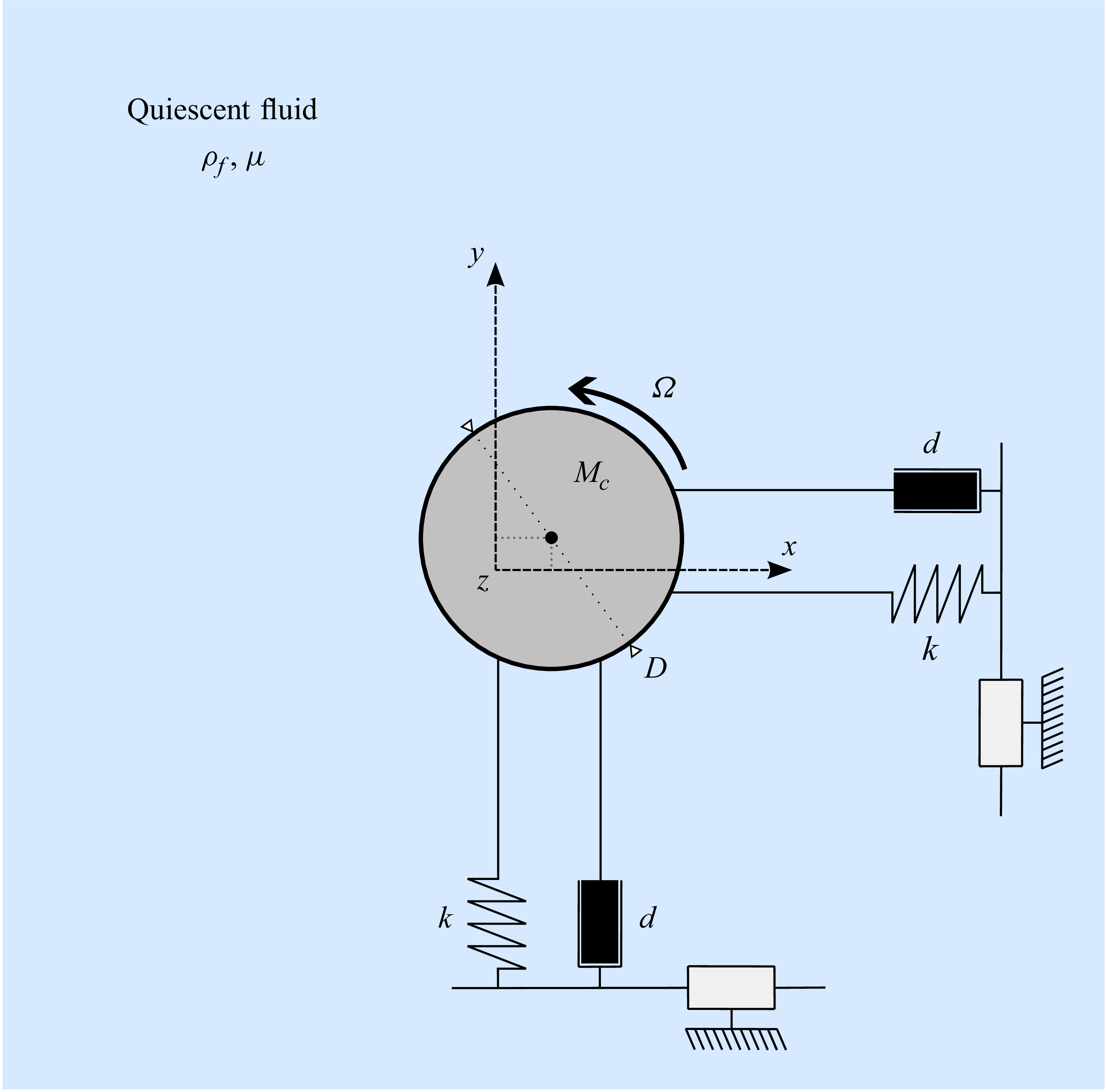

 ζx
 (Re,m⋆,U⋆)=(100,10,60)
 Np=5
 Δt=0.0025
 Np
 Δt
 R
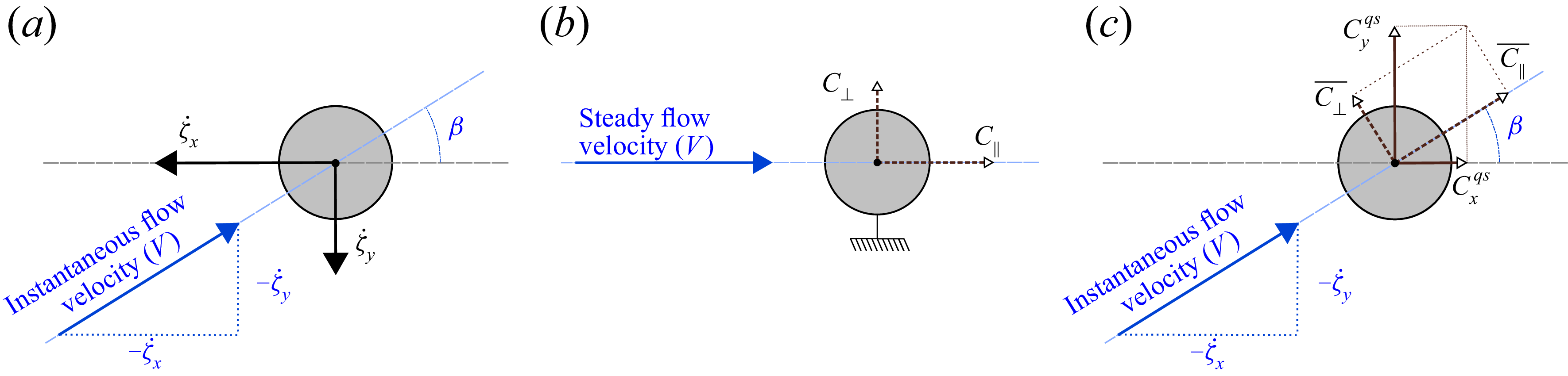
 V

 C∥¯=0
 C∥¯<0
 C∥¯
 V
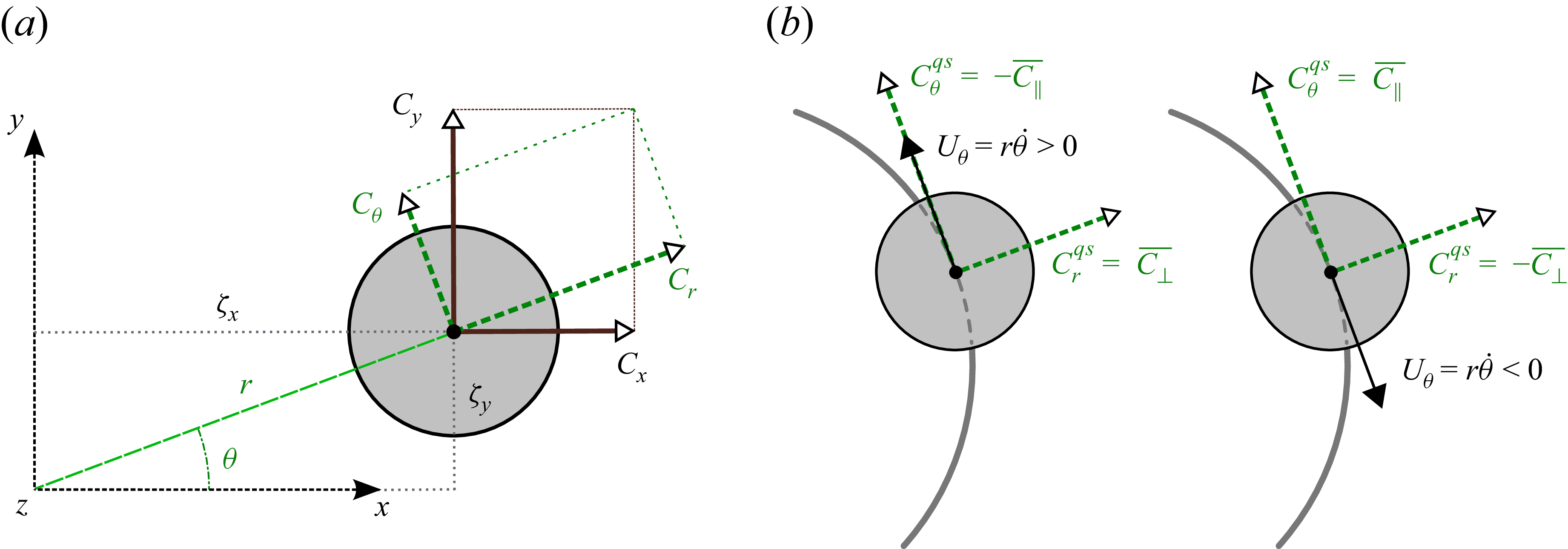

 x
 (Re,m⋆)=(50,10)
 U⋆=40
 U⋆=70
 U⋆=100
 +
 −
 M
 1

 (Re,U⋆)
 m⋆=10
 (m⋆,U⋆)
 Re=50
 +
 −
 m⋆

 x
 (Re,m⋆)=(50,10)
 U⋆=40
 U⋆=70
 U⋆=100
 1
 ωz∈[−0.02,0.02]
 1/fl

 (Re,m⋆)=(50,10)
 1
 −

 (Re,m⋆)=(50,10)
 r¯
 rh
 rl
 fζ
 fh
 fl
 1/fl
 U⋆∈{60,80,105}

 (Re,U⋆)
 m⋆=10

 (m⋆,U⋆)
 Re=50
 m⋆
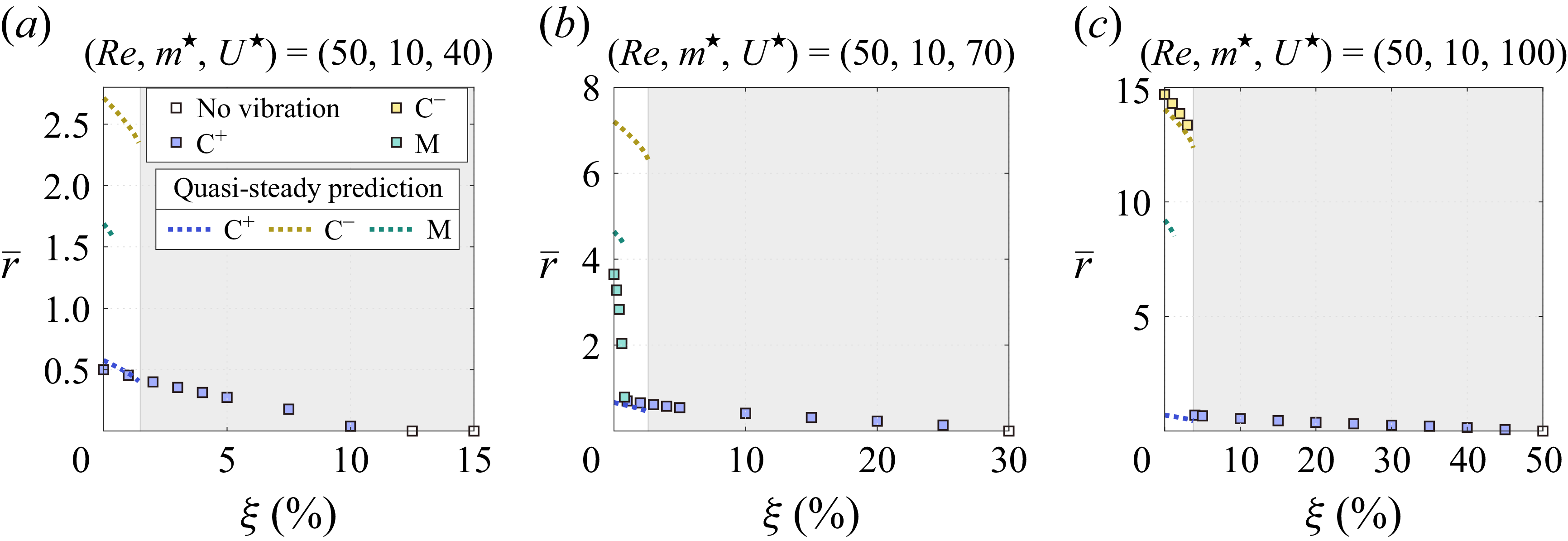
 (Re,m⋆)=(50,10)
 U⋆=40
 U⋆=70
 U⋆=100
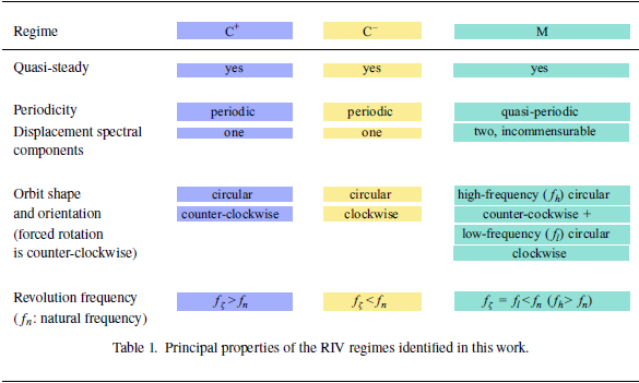

 x
 (Re,m⋆,U⋆)=(50,10,80)
 ζy(0)=0
 ζx(0)=0.05
 ζx(0)=5
 ζx(0)=9.22
 ζx(0)=15
 ζx(0)=20

 Open access

