1 Introduction
Disruptions of the plasma during the ramp of the current, leading to premature termination of the discharge, were observed early in tokamaks when the edge safety factor
 $q_{edge}$
passed through rational values
 $q_{edge}=m/n$
. The instabilities were in the form of a kinking of the plasma edge with a periodicity
 $n$
in the toroidal direction and
 $m$
in the poloidal direction. The
 $m>2$
instabilities and corresponding disruption could be avoided by reducing the rate of the current ramp. However, the
 $m/n=2/1$
mode at
 $q_{edge}=2$
could not be avoided so that
 $q_{edge}=2$
set a definite limit to the total current.
From considering a large aspect ratio cylindrical model with constant current density profile, the instabilities were identified by Shafranov (Reference Shafranov1970) as current-driven ideal magnetohydrodynamic (MHD) kink modes that are strongly peaked at the plasma edge. Later modelling by Wesson (Reference Wesson1978) showed that a diffuse current density profile is partly stabilizing and that the higher
 $m$
modes could be stabilized if
 $q_{edge}$
is sufficiently far from the corresponding rational. Nonetheless, the
 $2/1$
mode always remained unstable, consistent with the experimental observations.
Numerical calculations in full toroidal geometry and shaped cross-section confirmed this picture. The theory explained current ramp disruptions extremely well for tokamaks with a well-defined edge set by material limiters, and in particular the hard limit at
 $q_{edge}=2$
. The ideal external current-driven kink instability occurs in ranges of
 $q_{edge}$
,
 $$\begin{eqnarray}(m-1)<nq_{edge}^{crit}<nq_{edge}<m,\end{eqnarray}$$
with
 $q_{edge}^{crit}$
dependent essentially on the current density gradient in the edge region (Turnbull et al.
Reference Turnbull, Yasseen, Roy, Sauter, Cooper, Nicli and Troyon1989; Huysmans, Goedbloed & Kerner Reference Huysmans, Goedbloed and Kerner1993). A slower current ramp with higher
 $q_{edge/}q_{0}$
(
 $q_{0}$
is the on-axis safety factor) avoids the unstable regions and early limiter low
 ${\it\beta}$
discharges in DIII-D were subsequently found to be consistent with this picture (Turnbull et al.
Reference Turnbull, Yasseen, Roy, Sauter, Cooper, Nicli and Troyon1989, Reference Turnbull, Synder, Brennan, Chu and Lao2005).
However, with the development of large tokamaks with poloidal magnetic divertor boundaries (Meade et al.
Reference Meade, Arunasalam, Barnes, Bell, Bitter, Budny, Cecchi, Cohen, Daughney and Davis1980; Bol, Okabayashi & Fonck Reference Bol, Okabayashi and Fonck1985), the edge
 $q$
becomes mathematically infinite and the ideal theory would predict no ideal instability. Nevertheless, higher
 $(m,n)$
disruptions continued to occur in experiments during sufficiently fast current ramps (usually only
 $n=1$
disrupted, however), and the ultimate
 $2/1$
mode was observed empirically when
 $q$
at the 95 % poloidal flux surface, usually denoted
 $q_{95}$
, reached 2.0.
While the reason is not understood,
 $q_{95}$
in diverted plasmas has been found to play the same role that
 $q_{edge}$
plays in limited plasmas. Various explanations have been proposed over the past years but none appear to be very satisfactory. For example, an obvious resolution is that the 95 % flux surface is the real boundary of the plasma – that outside of this there is little current or pressure despite the closed flux surfaces. In that case, the observed mode would still be essentially an ideal kink mode. Alternatively, it is commonly supposed that the unstable ideal kink is converted to a resistive tearing mode (Wesson Reference Wesson1987; Medvedev et al.
Reference Medvedev, Martynov, Martin, Sauter and Villard2006) as the rational surface in the vacuum moves into the plasma. However, there is finite current and pressure in the edge region, at least to the edge of the pedestal, which is generally outside
 $q_{95}$
. The current density and pressure outside the 95 % surface is quite significant in
 $H$
-mode discharges. This is difficult to reconcile with
 $q_{95}$
being the effective plasma edge. For the tearing mode explanation, those instabilities are normally much more slowly growing than ideal kinks and are generally manifested as islands rotating and growing in the plasma, and then locking to the wall before disrupting. In contrast, the disruptions in divertor discharges as
 $q_{95}$
passes through rational values are fast growing, with growth rates at or near ideal levels (slowed usually by the nearby resistive wall), and do not exhibit any obvious island structure.
The conventional ansatz consisting of the substitution of
 $q_{95}$
for
 $q_{edge}$
appears to hold well in all cases where it has been carefully tested. More generally, no definite contradictions are known where
 $q_{95}<2$
in a stable free boundary discharge (although with stronger shaping and low aspect ratio,
 $q_{95}=3$
can present a limit before
 $q_{95}=2$
is reached (Turnbull et al.
Reference Turnbull, Yasseen, Roy, Sauter, Cooper, Nicli and Troyon1989)). The present paper provides an alternative explanation in the form of a hypothesis backed by numerical calculations from the MARS linearized MHD code (Bondeson, Vlad & Lutjens Reference Bondeson, Vlad and Lutjens1992). The observed instability in the diverted case is proposed to be due to destabilization of an external resistive kink mode as a result of the rapidly increasing plasma resistivity in the outer regions near the separatrix.
Fusion power in a magnetic confinement device scales with increasing plasma pressure according to
 $$\begin{eqnarray}P_{f}\sim {\it\beta}^{2}B_{0}^{4},\end{eqnarray}$$
where
 $B_{0}$
is the toroidal magnetic field strength at the centre of the plasma and
 ${\it\beta}\equiv {\it\mu}_{0}\langle p\rangle /B_{0}^{2}$
.
 $\langle p\rangle$
is the volume-averaged plasma pressure. In the absence of a stabilizing wall,
 ${\it\beta}$
is well known to be limited by MHD stability, as expressed by the Troyon limit (Troyon et al.
Reference Troyon, Gruber, Saurenmann, Semenzato and Succi1984)
 $$\begin{eqnarray}{\it\beta}\leqslant c_{T}\left(\frac{I}{aB_{0}}\right)=c_{T}\frac{S({\it\varepsilon},{\it\kappa},{\it\delta},\ldots )}{(aB_{0}q_{\ast })}.\end{eqnarray}$$
Here,
 $a$
is the minor radius,
 $I$
is the total plasma current and
 $c_{T}$
is the numerical Troyon coefficient found from stability calculations and confirmed experimentally to be typically in the range
 $2.5\leqslant c_{T}\leqslant 3.5$
if
 ${\it\beta}$
is expressed in percent. Thus,
 $c_{T}$
is the normalized
 ${\it\beta}$
, usually denoted
 ${\it\beta}_{N}$
. The function
 $S({\it\varepsilon},{\it\kappa},{\it\delta},\ldots )$
is a shape factor depending on inverse aspect ratio
 ${\it\varepsilon}\equiv (a/R)$
, elongation
 ${\it\kappa}$
and triangularity
 ${\it\delta}$
, and relatively weakly on higher order shaping (Lazarus et al.
Reference Lazarus, Navratil, Greenfield, Strait, Turnbull and Taylor1997). In (1.3),
 $q_{\ast }$
represents a value for the ‘edge’ safety factor (not to be confused with the ‘cylindrical’ safety factor, also commonly denoted as
 $q_{\ast }$
(Freidberg Reference Freidberg1987)). In a limiter discharge, this is
 $q_{edge}$
, but in a diverted discharge this is usually taken to be
 $q_{95}$
. In either case, fusion power is ultimately maximized with the strongest shaping and at the lowest
 $q_{\ast }$
.
An alternative strategy to increasing
 ${\it\beta}$
through optimizing
 $S$
and
 $q_{\ast }$
is to invoke stabilization from a nearby conducting wall. For a real resistive wall, this needs to be supplemented by active magnetic feedback on the time scale of the resistive decay of the wall image currents to suppress the remaining slowly growing resistive wall mode (RWM) (Freidberg Reference Freidberg1987; Zakharov & Putvinskii Reference Zakharov and Putvinskii1987). Alternatively, plasma rotation coupled to resonant kinetic stabilizing effects can provide at least partial stabilization (Strait et al.
Reference Strait, Taylor, Turnbull, Ferron, Lao, Rice, Sauter, Thompson and Wróblewski1995; Garofalo et al.
Reference Garofalo, Turnbull, Austin, Bialek, Chu, Comer, Fredrickson, Groebner, La Haye and Lao1999; Sabbagh et al.
Reference Sabbagh, Sontag, Bialek, Gates, Glasser, Menard, Zhu, Bell, Bell and Bondeson2006; Chu & Okabayashi Reference Chu and Okabayashi2010). Invoking wall stabilization effectively increases the Troyon coefficient
 $c_{T}$
, or
 ${\it\beta}_{N}$
. Active feedback stabilization schemes for suppressing the residual pressure-driven RWMs have been developed in both tokamaks and reversed field pinch (RFP) experiments (Chu & Okabayashi Reference Chu and Okabayashi2010) and wall stabilization has now been demonstrated many times showing steady operation with
 ${\it\beta}_{N}$
above the so-called ‘no wall’ or ‘free boundary’ limit – the limit predicted with no wall stabilization – in DIII-D (Strait et al.
Reference Strait, Taylor, Turnbull, Ferron, Lao, Rice, Sauter, Thompson and Wróblewski1995; Garofalo et al.
Reference Garofalo, Turnbull, Austin, Bialek, Chu, Comer, Fredrickson, Groebner, La Haye and Lao1999; Okabayashi et al.
Reference Okabayashi, Bialek, Chance, Chu, Fredrickson, Garofalo, Hatcher, Jensen, Johnson and La Haye2002; Strait et al.
Reference Strait, Bialek, Bogatu, Chance and Chu2003) and other experiments (Okabayashi et al.
Reference Okabayashi, Bol, Chance, Couture, Fishman, Fonck, Gammel, Heidbrink, Ida and Jaehning1987; Takeji et al.
Reference Takeji, Tokuda, Fujita, Suzuki, Isayama, Ide, Ishii, Kamada, Koide and Matsumoto2002; Hender et al.
Reference Hender, Gryaznevich, Liu, Bigi, Buttery, Bondeson, Gimblett, Howell, Pinches and de Baar2014; Sabbagh et al.
Reference Sabbagh, Sontag, Bialek, Gates, Glasser, Menard, Zhu, Bell, Bell and Bondeson2006; Chu & Okabayashi Reference Chu and Okabayashi2010).
The limit at
 $q_{edge}=2$
from current-driven external kinks, presents a comparable obstacle to increasing
 ${\it\beta}$
through increased current. Earlier experiments tried to exceed this current limit using a resistive wall to slow the mode growth (Stambaugh et al.
Reference Stambaugh, Allen, Bramson, Brooks, Burrell, Callis, Carlstrom, Chance, Chu and Colleraine1988; Chu & Okabayashi Reference Chu and Okabayashi2010). However, they were ultimately terminated by the growth of the subsequent current-driven RWM (Chu & Okabayashi Reference Chu and Okabayashi2010). Feedback stabilization of the current-driven external
 $2/1$
kink was first successfully demonstrated in the RFP RFX-mod (Martin et al.
Reference Martin, Apolloni, Puiatti, Adamek, Agostini, Alfier, Annibaldi, Antoni, Auriemma and Barana2009), operated as a tokamak. In the RFX-mod experiment, which employed 192 active coils, stabilization of the
 $m/n=2/1$
ideal external kink was achieved through wall stabilization to slow the mode growth to a resistive wall time, in combination with active feedback of the subsequent RWM (Piovesan et al.
Reference Piovesan, Hanson, Martin, Navratil, Turco, Bialek, La Haye, Lanctot, Okabayashi and Paz-Soldan2014). The relatively low
 ${\it\beta}$
discharge was operated with
 $q_{edge}$
decreasing below 2.0 during the current ramp to values of the order of
 $q_{edge}=1.6$
. The experiments were subsequently reproduced in DIII-D in both limited and diverted discharges (Hanson et al.
Reference Hanson, Bialek, Baruzzo, Bolzonella, Hyatt, Jackson, King, La Haye, Lanctot and Marrelli2014; Piovesan et al.
Reference Piovesan, Hanson, Martin, Navratil, Turco, Bialek, La Haye, Lanctot, Okabayashi and Paz-Soldan2014; Martin et al.
Reference Martin, Baruzzo, Bialek, Bolzonella, Bonfiglio, Cavazzana, Chacon, Ferraro, Garofalo and Hanson2015) using the full diagnostic suite available in DIII-D.
The experiments in the limited cross-section in DIII-D reached just below
 $q_{edge}\sim 2.0$
and the experiments in the diverted cross-sections reached below
 $q_{95}\sim 2.0$
. With no feedback, both discharge types disrupted violently due to the fast growing
 $2/1$
mode. With active feedback, the discharges could be maintained stably for many resistive wall decay times, though in all cases, control was ultimately lost (Hanson et al.
Reference Hanson, Bialek, Baruzzo, Bolzonella, Hyatt, Jackson, King, La Haye, Lanctot and Marrelli2014; Piovesan et al.
Reference Piovesan, Hanson, Martin, Navratil, Turco, Bialek, La Haye, Lanctot, Okabayashi and Paz-Soldan2014) due to technical limitations on the available power supplies.
In interpreting the DIII-D experiments, the role of
 $q_{95}$
becomes an acute issue. Ideal MHD has historically been absolutely successful in predicting the limit for limited discharges. In contrast, ideal MHD stability theory fails completely in predicting the observed instability for the diverted discharges with
 $q_{95}<2.0$
and
 $q_{edge}\gg 2.0$
. This is also clear from the simple application of the Shafranov theory, from previous numerical studies and is well confirmed in the present study. The subsequent analysis of the DIII-D experiments is consequently incomplete since no valid stability analysis is possible.
Clearly, an explanation is needed: apart from the
 $1/1$
external kink when
 $q<1$
everywhere (Shafranov Reference Shafranov1970), the
 $2/1$
ideal kink mode is the most gross instability possible, yet the ideal theory, which places the ideal plasma–vacuum transition at the diverted separatrix, fails to predict it at all in a diverted cross-section. The present paper addresses this issue directly using data from the experiments in DIII-D. A new, straightforward hypothesis is proposed and supported using numerical calculations. In ideal theory, the sharp transitions in stability as
 $q_{edge}$
passes through rational values are a manifestation of the idealized sharp transition in resistivity from zero to infinity assumed between the perfectly conducting confined plasma and the external infinitely resistive vacuum. In reality, of course, the very edge of the confined plasma region is highly resistive, with a resistivity profile
 ${\it\eta}$
varying with the electron temperature
 $T_{e}$
as
 ${\it\eta}\sim T_{e}^{-3/2}$
. This yields typically a steeply rising profile within a narrow region from somewhere outside the 95 % flux surface up to the last closed flux surface. The hypothesis then proposes that when the
 $q=2$
surface falls in the highly resistive edge region, the ideal kink that would be unstable if the
 $q=2$
surface were in the vacuum is converted to a resistive kink. Essentially, the high resistivity in the edge region appears like a vacuum as far as the kink instability is concerned.
In a systematic study of the complex resistive MHD spectrum in generic tokamak equilibria (Huysmans et al. Reference Huysmans, Goedbloed and Kerner1993), the resistive external kink was considered as an explanation for observed kink modes in a variety of situations. In that work, the plasmas were limited and the resistivity profile was generally kept constant across the plasma. The present study is intended to focus specifically on the diverted plasma case under experimental conditions where the discrepancy with ideal MHD theory is most dramatic. Nevertheless, the results are qualitatively consistent with those obtained by Huysmans et al.
In the present work, a definite distinction is made between a tearing mode and a resistive kink. The two have distinctly different parity at the rational surface – the kink has interchange parity where the two adjacent surfaces interchange, as opposed to tearing apart. In practice, at finite
 ${\it\beta}$
, the exhibited instabilities will have some mixed character. In Huysmans et al. (Reference Huysmans, Goedbloed and Kerner1993), the instabilities tended to be a mixture of tearing and interchange parity but, depending on
 $q_{edge}$
, one parity was often dominant. In the results here for the
 $2/1$
external kink, the interchange parity is completely dominant. The resonant components of the displacement peak near the
 $q=2$
surface, so that the neighbouring surfaces are interchanging (the peak moves faster than the neighbouring surfaces), instead of changing sign as is the case for a tearing mode where the rational surface tears apart. It is in this sense that the instabilities are referred to as resistive kinks.
The analysis is based on data obtained from the DIII-D low
 $q$
experiments, and using equilibria reconstructed from the available diagnostic data. Section 2 discusses the experiments briefly, focusing specifically on the aspects of interest here, including the equilibrium reconstructions. The analysis is restricted to the
 $n=1$
,
 $m=2$
mode and the
 $q=2$
limit since good data are available from the experiments but the results are expected to be broadly applicable to higher
 $n$
and
 $m$
. More important, the analysis is for
 $L$
-mode plasmas, again since good quality data were available for comparison. Nevertheless, it is expected that the results should generally apply in
 $H$
-mode as well.
The stability calculations are described in § 3. The strategies that have been developed for dealing with the diverted outer surface are reviewed in § 3.1. The calculations for the limited discharge are described in § 3.2, where it is shown that ideal MHD works well, although with one minor discrepancy that can, in fact, be explained within the context of the model. Section 3.3 describes the stability calculations for the diverted case. In all cases considered, the calculations that include the
 $q=2$
surface within the plasma predict stability to the
 $2/1$
external kink. Including a resistivity profile is shown to yield an instability that is largely indistinguishable from an ideal external kink. Three different models for the profile are considered. The result is somewhat sensitive to the resistivity and some enhancements near
 $q=2$
are generally found to be necessary if otherwise realistic profiles are assumed.
Section 4 provides a general discussion. In light of the results from § 3, several interesting aspects are worth commenting on. Most notably, the results can also explain the previously puzzling observation (Hanson et al.
Reference Hanson, Bialek, Baruzzo, Bolzonella, Hyatt, Jackson, King, La Haye, Lanctot and Marrelli2014; Piovesan et al.
Reference Piovesan, Hanson, Martin, Navratil, Turco, Bialek, La Haye, Lanctot, Okabayashi and Paz-Soldan2014; Martin et al.
Reference Martin, Baruzzo, Bialek, Bolzonella, Bonfiglio, Cavazzana, Chacon, Ferraro, Garofalo and Hanson2015) that the instability in the limited discharges actually appears slightly before the discharge reaches
 $q_{edge}=2$
. A detailed discussion of this is provided in § 4.1. The scaling with resistivity is treated in § 4.2. Justifications for the modifications are given in § 4.3. Section 4.4 then discusses the credibility of alternative explanations; § 4.4.1 discusses the possibility of tearing modes in the experiments and the complications from internal kink and other ideal instabilities are dealt with in § 4.4.2.
Final concluding remarks are made in § 5. Section 5.1 discusses some open questions and future directions that could be pursued. Finally, the work has interesting implications for projections of ITER performance based on scaling with
 $q_{95}$
. These speculations are considered in § 5.2.
2 Low
 $q$
operation in DIII-D

The results from the DIII-D low
 $q$
experiments have been reported extensively from the point of view of the feedback stabilization (Hanson et al.
Reference Hanson, Bialek, Baruzzo, Bolzonella, Hyatt, Jackson, King, La Haye, Lanctot and Marrelli2014; Piovesan et al.
Reference Piovesan, Hanson, Martin, Navratil, Turco, Bialek, La Haye, Lanctot, Okabayashi and Paz-Soldan2014). To summarize these aspects briefly in order to provide context for the work here, several discharges with low edge
 $q$
were produced over several days of runtime, and covering Limiter
 $L$
-mode, Diverted
 $L$
-mode and Diverted
 $H$
-mode conditions; in comparison, the original RFX-mod experiments were done in Ohmic conditions. Feedback stabilization was successful under
 $L$
-mode conditions but the Diverted
 $H$
-mode discharges were only successful in reaching
 $q_{95}=2$
in two cases. This was due essentially to operational constraints; sawteeth and edge localized modes (ELMs) typically appeared at the L–H transition well before low
 $q$
was reached and the feedback control system had difficulty discriminating this activity from the external kink so that ultimately control was lost. Even in the successful
 $H$
-mode experiments, the data are complicated by the ELM activity. Since a direct one-to-one comparison can be made, the present analysis is therefore restricted to the
 $L$
-mode diverted and limited discharges. The feedback aspects are also largely ignored and the focus is on the instabilities that appear under open-loop conditions.
Figure 1 shows the time development of the
 $L$
-mode Limiter cross-section DIII-D discharge no. 154 907. The current and
 $q_{edge}$
are given in figure 1(a,b), showing
 $q_{edge}$
decreasing toward 2.0 until the
 $2/1$
mode onset at 2425 ms and the subsequent complete disruption at 2700 ms. The
 $2/1$
precursor to the disruption is not always observed, nor is usually so prominent as in this case. The mode rotates in the electron diamagnetic direction (opposite the plasma rotation direction). The precursor magnetic signals are displayed in figure 1(c) on an expanded scale. This shows the perturbed poloidal field from 50 poloidal field probes with the mode phase given by the dashed line and the amplitude by the solid line (black) plotted on an exponential scale. The growth time (dotted red curve) is found to be 1.8 ms, comparable to the wall resistive time of about 2.5 ms. The mode amplitude is also shown in figure 1(d) as colour contours versus time and toroidal phase. The mode has a clear
 $2/1$
structure with all the usual features expected of the unstable ideal external kink.
Time development of the DIII-D
 $L$
-mode limited discharge no. 154 907 showing (a) current
 $I$
and (b) edge safety factor
 $q_{edge}$
. (c) Amplitude (solid black curve, left logarithmic scale) and phase (dashed blue curve, right linear scale) of magnetic precursor signals on an expanded time scale. The red dashed curve is the 1.8 ms growth curve. (d) Colour contours of amplitude versus toroidal angle and time on expanded time scale.

The discharge equilibria were reconstructed for times approaching the
 $2/1$
mode onset using the EFIT code (Lao et al.
Reference Lao, Ferron, Groebner, Howl, St. John, Strait and Taylor1990) and fitted to all available external magnetic data, internal motional Stark effect (MSE) data and kinetic pressure data from Thomson scattering and charge exchange recombination (CER) measurements. These were coupled with transport simulations to obtain the fast ion pressure from the ONETWO code (Pfeiffer et al.
Reference Pfeiffer, Davidson, Miller and Waltz1980; St. John et al.
Reference St. John, Taylor, Lin-Liu and Turnbull1994). Operationally in these discharges, the current is ramped in order to reach low
 $q_{\ast }$
(
 $q_{\ast }=q_{edge}$
or
 $q_{\ast }=q_{95}$
). Current diffusion redistributes the inductive current into the core, thus lowering
 $q$
everywhere. By applying a sufficiently fast current ramp, the discharge was designed to reach
 $q_{edge}=2$
before the onset of sawtoothing when the safety factor on axis
 $q_{0}\leqslant 1$
. This was intended to avoid the effects of sawteeth on confinement, and because sawteeth often trigger other instabilities, particularly neoclassical tearing modes (NTMs) (Sauter et al.
Reference Sauter, Westerhof, Mayoral, Alper, Belo, Buttery, Gondhalekar, Hellsten, Hender and Howell2002). In addition, feedback control could not always discriminate the
 $1/1$
magnetic signals from the external kink.
Nevertheless, sawteeth did often occur since the current ramp rate was limited in order to avoid triggering the higher
 $n$
and
 $m$
external kink modes, so that
 $q_{0}=1$
was often reached before
 $q_{edge}=2$
. To maintain
 $q_{0}>1$
in the stability calculations and avoid the ideal internal kink (Shafranov Reference Shafranov1970; Bussac et al.
Reference Bussac, Edery, Pellat and Soule1976), a simple expedient of ignoring the radial electric field correction (Rice et al.
Reference Rice, Burrell, Lao and Lin-Liu1997) to the MSE data in the reconstructions was applied. This was usually sufficient to keep
 $q_{0}>1$
. However, this results in the reconstructions typically having an off axis minimum safety factor,
 $q_{min}$
, with
 $q_{0}>q_{min}>1.0$
, but still within the estimated experimental uncertainties.
The reconstruction at 2425 ms is shown in figure 2 with (a) the reconstructed boundary and flux surfaces and (b) the safety factor and (c) toroidal current density profiles. This reconstruction, right at the mode onset, yielded a value for
 $q_{edge}$
of
 $q_{edge}=2.08\pm 0.01$
. Note in particular the slightly hollow
 $q$
. Subsequent ideal MHD stability calculations using the GATO code (Bernard, Helton & Moore Reference Bernard, Helton and Moore1981) for this equilibrium found complete stability, consistent with
 $q_{edge}>2.0$
. This was confirmed with the DCON (Glasser Reference Glasser1997) and MARS (Bondeson et al.
Reference Bondeson, Vlad and Lutjens1992) codes. The DCON calculations show the positive perturbed energy decreasing uniformly as the mode onset time is approached (Hanson et al.
Reference Hanson, Bialek, Baruzzo, Bolzonella, Hyatt, Jackson, King, La Haye, Lanctot and Marrelli2014), indicating the approach to an ideal instability.
Reconstructed equilibrium for the limited discharge no. 154 907 at 2425 ms with
 $q_{edge}=2.08$
. (a) Boundary and reconstructed flux surfaces with model wall for reference, (b) safety factor and absolute value of the pressure gradient as functions of
 $\sqrt{V}$
and, (c) toroidal current density profile as a function of major radius. Shown also in (b) and (c) are the extrapolated equilibrium profiles projected beyond 2425 ms to
 $q_{edge}=1.95$
, denoted as 2650 ms.

To obtain a later equilibrium from the early mode onset phase when
 $q_{edge}<2.0$
, reconstructions were made by extrapolating the profiles forward in time to higher current but using the plasma boundary from 2425 ms. This yielded equilibria with decreasing
 $q_{edge}$
, and for a small but significant extrapolation, equilibria similar to that in figure 2 were obtained with
 $q_{edge}\sim 1.95$
for ideal stability analysis with the GATO code (Bernard et al.
Reference Bernard, Helton and Moore1981). A slightly different procedure was also employed whereby the original equilibrium at 2425 ms was recomputed as a fixed boundary inverse equilibrium using the CHEASE code (Lutjens, Bondeson & Sauter Reference Lutjens, Bondeson and Sauter1996), slightly cut off to remove the X-point, with the same profiles but with
 $I$
readjusted to set
 $q_{edge}<2$
. The two schemes yielded similar results.
The extrapolated profiles for the limiter discharge no. 154 907 with
 $q_{edge}=1.95$
are also shown overlaid in figure 2(b,c). Compared to the reconstruction at 2425 ms (solid curves), the extrapolated
 $q$
profile (dashed curve) is similarly slightly hollow but with the minimum further out in radius. The profile extrapolation procedure tended to produce equilibria with even more hollow
 $q$
profiles than the original. The minor complications that consequently arise in the analysis and interpretation of the results will be discussed in some detail in § 4. Nevertheless, the results can reproduce the observed ideal instabilities. The only significant difference between the profiles in figure 2 is the edge
 $q$
below 2.0 in the extrapolated equilibrium.
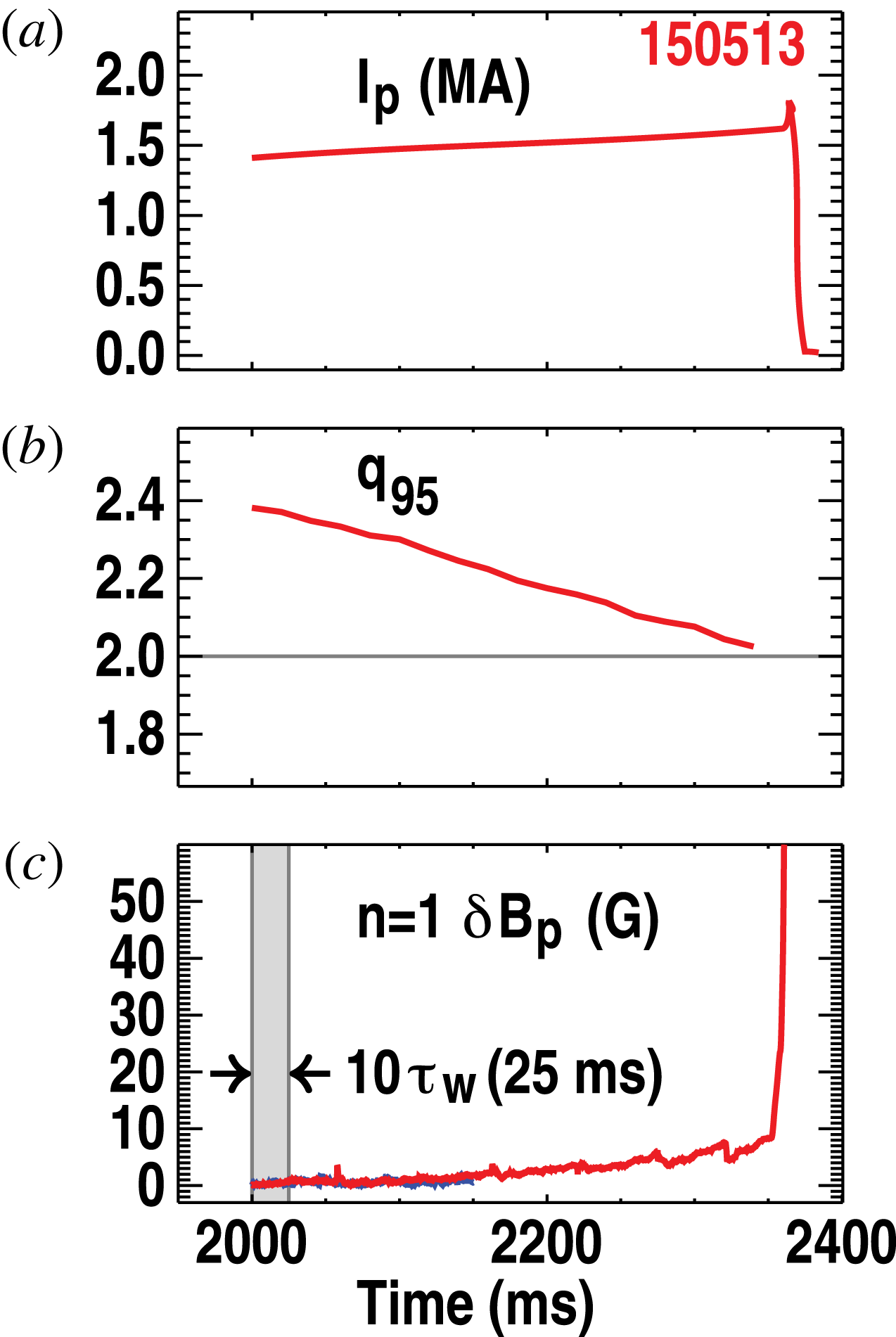
The diverted
 $L$
-mode discharge no. 150 513 similarly underwent a fast
 $2/1$
disruption but at
 $q_{95}=2$
. Figure 3 shows the time trace for this discharge for comparison with figure 1, with
 $I$
ramped up and
 $q_{95}$
dropping to
 $q_{95}=2$
. In this case, there was no discernible oscillating magnetic precursor to the instability onset. Figure 4 shows the reconstructed equilibrium at 2340 ms, just before the observed mode onset. The major difference compared to figure 2 is the upper single null (USN) divertor shape. The differences in the profiles are largely a result of this shape change. Note that the reconstructed profiles in both limiter and divertor cases generally have a finite edge pressure gradient so there is always some current density on the last closed flux surface, even when the average over the surface is small. The finite edge pressure gradient is a measured feature present in the raw data. The gradient in the surface-averaged current density is also finite in most of the reconstructions. From the reconstruction for discharge no. 150 513 at 2340 ms,
 $q_{95}=2.06$
. As will be discussed later in § 3.1, numerically, a finite value is found for
 $q_{edge}$
with
 $q_{edge}\sim 5$
.
Time development of DIII-D
 $L$
-mode diverted discharge no. 150 513 showing (a) current
 $I$
, (b) the safety factor at the 95 % flux surface
 $q_{95}$
, and (c) poloidal magnetic field sensor signal.

Reconstructed equilibrium for the diverted discharge no. 150 513 at 2340 ms with
 $q_{95}=2.06$
and
 $q_{edge}=5.35$
. (a) Boundary and reconstructed flux surfaces with model wall for reference, (b) safety factor and pressure gradient profiles as functions of
 $\sqrt{V}$
and (c) toroidal current density as a function of major radius. Shown overlaid in (a) is the equilibrium boundary obtained from the CHEASE code with a cut off of the edge to exclude the X-point (red dashed curve), yielding
 $q_{95}=1.995$
and
 $q_{edge}=2.85$
. The corresponding profiles are also overlaid (dashed curves) in (b) and (c).

Except for the lack of any obvious precursor, the disruption in discharge no. 150 513 at 2340 ms shows all the same features of the ideal kink disruption as in discharge no. 154 907. In particular, in both discharges, there is no sign of tearing at internal rational surfaces (
 $q=2$
in the diverted case), no precursor mode locking, and the growth rates are consistent with the fastest resistive wall time, somewhat faster than a typical tearing mode. With one caveat to be discussed in § 4.4.1, there is also no clear evidence of temperature flattening indicative of island formation at onset or in the early growth phase.
Nevertheless, in contrast to the limiter discharge no. 154 907, all ideal stability calculations for discharge no. 150 513 find complete stability to the
 $m/n=2/1$
external kink. For the reconstruction at 2340 ms,
 $q_{95}=2.06$
, which, as for discharge no. 154 907, is slightly on the (experimentally) expected stable side of the marginal point, so the stability is not surprising. However, even when the procedure of extrapolating the profiles slightly forward in time to yield equilibria with
 $q_{95}<2$
was applied, the calculations continued to yield complete stability to the
 $2/1$
external kink. With variations in the fitting, cutoff, and extrapolation procedures, the only unstable ideal modes found were internal kinks and very weakly unstable, highly edge localized,
 $m\geqslant 3$
peeling modes in narrow ranges of
 $q_{edge}$
. The stability calculations will be discussed in the next section.
3 External kink stability in limiter and divertor configurations
The conclusion that ideal MHD works extremely well in the limiter case, yet fails completely for all plausible reconstructions in the divertor case rests on the validity of the equilibrium reconstructions and the subsequent ideal MHD stability evaluation. These generate several numerical issues that need to be addressed. The key issue is the treatment of the singularity at the X-point of the diverted separatrix and will be discussed in the following subsection in detail. Also, the complications arising from coupling between the external kink modes of interest and the ideal internal kink will be discussed briefly at the end of § 3.1 and later in § 4.4.
3.1 Numerical issues
The poloidal field at the X-point in a divertor configuration vanishes, leaving a saddle point in the poloidal plane and a purely toroidal field. No special behaviour appears in the vicinity of the X-point in strictly two dimensions, though with three-dimensional (3-D) perturbations, the singular behaviour is manifested as Hamiltonian chaos with a complex web of homoclinic tangles (Evans et al.
Reference Evans, Moyer, Burrell, Fenstermacher, Joseph, Leonard, Osborne, Porter, Schaffer and Snyder2006). Nevertheless, the X-point is a coordinate singularity and needs to be handled properly. Even though there seems to be no new (non-ideal MHD) physics associated with the singularity, it does present numerical difficulties for quantities such as
 $q$
that involve surface integrals of
 $B_{pol}^{-1}$
. In particular, for inverse equilibrium codes based on flux coordinates, such as the CHEASE code (Lutjens et al.
Reference Lutjens, Bondeson and Sauter1996), the Jacobian is usually singular (for example if an equal arclength poloidal angle is used) and the coordinate system can become highly distorted in the neighbourhood of the X-point (for straight field line coordinates). For direct equilibrium codes such as EFIT (Lao et al.
Reference Lao, Ferron, Groebner, Howl, St. John, Strait and Taylor1990), the singularity is less serious but still requires care.
For stability codes based on a flux coordinate system, the singularity needs to be handled carefully. Two schemes are usually employed – both essentially remove the singular point. In the first approach, the plasma boundary is moved slightly inward so that the X-point lies outside the region considered as plasma. This cutoff procedure is required in numerical calculations that use a Fourier representation in the poloidal angle, but has traditionally been deployed in different ways in different codes – the differences typically being whether the current density and pressure in the removed region are shifted back into the plasma to keep
 $I$
and
 ${\it\beta}$
fixed, or are removed completely, and whether force balance is reimposed on the modified plasma profiles.
The MARS (Bondeson et al.
Reference Bondeson, Vlad and Lutjens1992) and DCON (Glasser Reference Glasser1997) stability calculations use variations of this cutoff procedure. The equilibria for MARS are recomputed with fixed current density, pressure and boundary shape using the inverse equilibrium code CHEASE (Lutjens et al.
Reference Lutjens, Bondeson and Sauter1996), whereas DCON can either use the CHEASE equilibrium or employ a simple cutoff of the edge current and pressure from the original reconstructed direct equilibrium. The resulting
 $q_{edge}$
is finite but the numerical value depends clearly on how much plasma is cut off. For sufficiently small cutoffs, the different procedures usually result in negligible changes in the results and a consistent answer can be obtained. For larger cutoffs, where significant current density and pressure need to be redistributed, or where a low-order rational surface is removed, the results are sensitive to the cutoff.
The alternative procedure, used in the ERATO (Gruber et al.
Reference Gruber, Troyon, Rousset, Kerner and Bernard1981), GATO (Bernard et al.
Reference Bernard, Helton and Moore1981) and KINX (Degtyarev et al.
Reference Degtyarev, Martynov, Medvedev, Troyon, Villard and Gruber1997) codes, and also effectively in the M3D-C
 $^{1}$
code (Ferraro, Jardin & Snyder Reference Ferraro, Jardin and Snyder2010), utilizes a finite element representation in the poloidal angle. With a suitable choice of Jacobian (e.g. with an equal arclength poloidal angle), the distortion of the poloidal coordinate lines in the region around the X-point is minimized. Although the Jacobian is still singular at the X-point, the logarithmic singularity is weak and is manifested in surface integrands of the form
 $\langle F\rangle =\oint F(l)\,\text{d}l/B_{pol}$
, where
 $l$
is the arclength. Discrete numerical integration then yields finite numbers for these divergent integrals if the singular point where
 $B_{pol}\rightarrow 0$
is not a grid point. For example, in the case of the edge safety factor,
 $q=(f/2{\it\pi})\oint R\,\text{d}l/B_{pol},(f=RB_{{\it\varphi}})$
the numerical integration in the GATO code yields
 $q_{edge}\sim 5$
for the EFIT equilibrium reconstructed from discharge no. 150 513 at 2340 ms. The finite value is, in fact, set largely by how close the 2-D interpolation procedure can approximate the zero gradient in flux at the X-point rather than the fineness of the integration grid. The M3D-C
 $^{1}$
code also uses essentially the same method; it solves for the perturbed fields in the entire plasma plus vacuum region but avoids calculation of singular surface integrals.
It should be emphasized that the explicit cutoff and the finite (approximate) numerical integration procedures are different. The former explicitly either removes or redistributes pressure and current but the latter does not. The effect of the explicit cutoff has been investigated systematically with KINX in a comparison of the two approaches (Medvedev et al.
Reference Medvedev, Hender, Sauter and Villard2001). The conclusion from that work was that the results with no cutoff can be qualitatively different from those that employed an explicit cutoff. A reasonable summary of the situation, consistent with the present and other studies, is that the cutoff matters each time it removes a significant rational surface from the edge. While there are, of course, infinitely many rational surfaces in principle, only the very low order surfaces produce a significant instability. For the low order surfaces, the difference between including the surface in the plasma and removing it is simply that the former is stable but the latter unstable to the corresponding
 $m/n$
external kink.
In the present case, it means simply that the
 $q=2$
surface cannot be removed without an expectation that it will affect the stability. From sensitivity studies with respect to variations within experimental uncertainties in the edge profiles, no unstable ideal external kink instabilities with significant
 $m=2$
could be found using the ideal GATO code for discharge no. 150 513 using reconstructed equilibria. From studies of different cutoffs, it was found that the
 $q=2$
surface must be removed in order to find the unstable ideal external
 $2/1$
kink. However, this would require 5 % of the plasma to be cut off. Different cutoffs, provided they were less than a tenth of a percent of the poloidal flux, yielded consistent results except in the narrow ideally unstable
 $q_{edge}$
ranges just below rational values. As will be discussed in § 4.4, these instabilities cannot easily explain the observed disruption. In contrast, the MARS and DCON codes utilizing a cutoff of 0.3 % provided by the CHEASE code find an edge
 $q$
just below 3. This might be expected to drive an edge 3/1 external kink or peeling mode but MARS and DCON, as well as GATO also find the equilibrium to be stable. Thus, the disagreement with the experimentally observed instability remains to be resolved.
The second numerical issue is only a technical complication, though also with possible consequences in practice. It applies in both the limiter and divertor configurations. As discussed in § 2, the equilibria are reconstructed so that
 $q_{min}>1$
is maintained. The classic internal kink with
 $q_{min}<1$
(Shafranov Reference Shafranov1970; Bussac et al.
Reference Bussac, Edery, Pellat and Soule1976) is then generally avoided. The safety factor profile is then usually slightly non-monotonic and this tends to destabilize the ideal quasi-interchange mode (Wesson Reference Wesson1986) if
 $q_{min}\leqslant 1+{\it\varepsilon}\;({\it\varepsilon}\sim a/R)$
. In some of the equilibria used in the study, this internal mode is unstable. This is an independent purely
 $1/1$
mode but can also couple to the external kink to produce coupled
 $1/1$
and
 $2/1$
modes at finite
 ${\it\beta}$
. The external kink component of interest can become dominated by the internal
 $1/1$
displacement since the
 $1/1$
mode is easily excited to large amplitudes by a small energy imbalance. The calculations have been repeated for a number of different reconstructions with varying
 $q_{0}$
and
 $q_{min}$
, and the external kink modes have varying contributions from the
 $1/1$
component. The issue then is just interpretation; can the instability be characterized as a predominantly
 $2/1$
mode rather than a
 $1/1$
mode. The quasi-interchange can usually be eliminated by raising
 $q_{min}$
further. Normally, the judicious selection of an appropriate equilibrium reconstruction or time slice with sufficiently high
 $q_{min}$
is enough to ensure the
 $2/1$
component is unambiguously dominant.
The stability calculations are discussed separately for the limiter and divertor configurations in the following two sections. The ideal calculations were generally performed using the GATO code, employing no cutoff, but a numerically discrete and finite integration on the diverted surface. The ideal results were confirmed using MARS, DCON, and M3D-C
 $^{1}$
. Resistive MHD calculations were performed using the MARS code. Here, for the diverted case, an equilibrium recomputed from the CHEASE code was used with the boundary taken at the 99.7 % poloidal flux surface, and the value
 $q_{edge}\sim 2.85$
, well above 2.0, was obtained. The CHEASE equilibrium is shown overlaid in figure 4 with the original reconstructed equilibrium. Although the cutoff did not destabilize the
 $m/n=3/1$
ideal external kink, a significant and often dominant
 $m=3$
, as well as higher
 $m$
harmonics, were always present in the resistive MHD calculations. This will be discussed. No cutoff was required in the limiter case except to artificially reduce
 $q_{edge}$
slightly to a value below 2.
Several comments should be made regarding the stability calculations. The ideal calculations with the GATO code generally assumed a wall at infinity since the aim is to show that no ideal mode is unstable in the diverted case. On the other hand, the resistive MARS calculations assumed a resistive wall at the location of the DIII-D vacuum vessel in order to reproduce the instability under experimental conditions. The wall time was taken to be
 $2.78\times 10^{4}$
plasma Alfvén times, which is the standard value used for DIII-D. This yields an actual resistive wall time of around 9 ms. Recent careful studies, however, have found this to be a factor two longer than the value that provides the closest match to the vacuum field decay time for
 $n=1$
fields (Hanson et al.
Reference Hanson, Bialek, Turco, King, Navratil, Strait and Turnbull2016) (the actual wall times depend weakly on the mode in question). While the actual growth rates are unimportant here, some calculations were nevertheless repeated with no wall to verify that the growth rates are at ideal levels. Finally, in all cases, the density was assumed constant for simplicity. A profile in density changes only the growth rates, with a small effect on the mode structure. Again, the magnitude of the linear growth rates is relatively unimportant here. The effect on mode structure could make a difference in the experimental diagnostic comparisons, but, again, the effect should be small.
3.2 Limiter configuration
Ideal stability calculations using the GATO code for the reconstructed limiter discharge no. 154 907 at 2425 ms with
 $q_{edge}=2.08$
found complete stability even with no stabilizing wall. This was confirmed with DCON and MARS. Variations in the detailed edge conditions also found stability unless the edge
 $q_{edge}$
was reduced below 2.0 from the best-fit value of
 $q_{edge}=2.08$
. This result is completely consistent with the ideal theory.
The ideal
 $n=1$
stability calculations were performed using GATO for the same discharge no. 154 907 at a slightly extrapolated time, where
 $q_{edge}=1.95$
. The extrapolation was performed by projecting the profiles to slightly higher current, while keeping the remaining data to be fitted, including the plasma boundary, unchanged. With a perfectly conducting wall on the plasma the equilibrium is unstable to an internal
 $m=1$
quasi-interchange mode due to the slightly hollow
 $q$
profile. With no wall, a pair of unstable ideal free boundary modes was found. Figure 5 shows the two modes. Plotted is the Fourier decomposition of the normal displacement
 $X\equiv {\it\xi}\boldsymbol{\cdot }\boldsymbol{{\rm\nabla}}{\it\psi}$
with respect to the PEST straight field line angle
 ${\it\chi}_{P}$
, as a function of
 $\sqrt{V}$
, with
 $V$
the normalized volume contained within a given flux surface. The real and imaginary parts are different since the equilibrium is vertically asymmetric but both show
 $m=1$
coupled to a significant
 $m=2$
component with different phases. Note also the different scales between (a) and (b) and between (b) and (c); the overall amplitude for each independent eigenmode is arbitrary, however. The respective no wall growth rates are
 ${\it\gamma}{\it\tau}_{A}=0.00752$
and
 ${\it\gamma}{\it\tau}_{A}=0.001575$
(
 ${\it\tau}_{A}\equiv \sqrt{B_{0}^{2}/{\it\mu}_{0}{\it\rho}R_{0}^{2}}$
is the Alfvén time, with
 ${\it\rho}$
the mass density). The
 $2/1$
external kink is destabilized when the wall is removed and couples to the quasi-interchange to produce two separate independent linear combinations of the external and internal modes. The relative contributions from the coupled
 $1/1$
and
 $2/1$
system depend on the reconstruction details but the
 $m/n=2/1$
kink component is the driving instability of the external mode.
Ideal eigenmodes computed using GATO showing the Fourier decomposition of the normal displacement
 $X\equiv {\it\xi}\boldsymbol{\cdot }\boldsymbol{{\rm\nabla}}{\it\Psi}$
with respect to the PEST straight field line poloidal angle
 ${\it\chi}_{P}$
, as a function of
 $\sqrt{V}$
, for the two unstable ideal modes found in the limited discharge no. 154 907 near 2425 ms. The equilibrium used is the extrapolated time shown in figure 2. Shown are (a) and (c) the real and (b) and (d) imaginary parts of the two modes. Note the normalization chosen with
 $\max _{{\it\Psi},m}|Re(X({\it\Psi},m))|^{2}\equiv 1$
results in different scales between the real and imaginary components for each separate eigenmode.

The presence of multiple harmonics and the inclusion of a sizeable
 $m=n=1$
component are inessential details for the purpose of identifying the disruption cause. Slightly different extrapolation procedures also yield different mixes of poloidal harmonics but all have an
 $m/n=2/1$
external kink coupled to an
 $m/n=1/1$
internal kink. The key point is that the predicted instability is consistent with the observed disruption to within a small margin of error.
The MARS code, running under ideal MHD conditions, reproduced the external
 $m/n=2/1$
kink with
 $q_{edge}<2$
, utilizing an equilibrium from the CHEASE code (Lutjens et al.
Reference Lutjens, Bondeson and Sauter1996) that was obtained from the initial EFIT reconstruction at 2425 ms but with a slightly increased total current chosen to reduce
 $q_{edge}$
to
 $q_{edge}=1.995$
. The calculations again found a linearly unstable
 $2/1$
mode. In this equilibrium, the internal
 $m/n=1/1$
quasi-interchange was stable and only one unstable external mode was found. Figure 6(a) shows the measured signals from the external magnetic probes located at the wall at 2456 ms. A synthetic diagnostic prediction of these signals was made (Hanson et al.
Reference Hanson, Bialek, Baruzzo, Bolzonella, Hyatt, Jackson, King, La Haye, Lanctot and Marrelli2014) using the result from the MARS code (Bondeson et al.
Reference Bondeson, Vlad and Lutjens1992) with no wall and is replicated in figure 6(b). The observed
 $2/1$
structure of figure 6(a) is well reproduced.
(a) Measured and (b) predicted synthetic diagnostic magnetic signals at the wall for the limited DIII-D discharge no. 154 907. The prediction using the MARS code, reproduced from (Hanson et al.
Reference Hanson, Bialek, Baruzzo, Bolzonella, Hyatt, Jackson, King, La Haye, Lanctot and Marrelli2014), is from the equilibrium with
 $I$
increased to reduce
 $q_{edge}$
to
 $q_{edge}=1.995$
.

The conclusion for the limiter discharge, no. 154 907 is, as expected, that ideal MHD stability predicts the onset of the
 $2/1$
external kink mode at
 $q_{edge}=2.0$
, close to the observed onset at
 $q_{edge}=2.08$
. Analysis of similar discharges in the same series finds essentially identical behaviour. The predicted ideal kink mode structure also agrees well with the external magnetic signals for this discharge and the growth rate is consistent with an expected
 $2/1$
ideal MHD mode growing on the resistive wall time scale. One apparently minor point is the estimated onset actually appears to be slightly above
 $q_{edge}=2.0$
, outside the estimated experimental uncertainty (Hanson et al.
Reference Hanson, Bialek, Baruzzo, Bolzonella, Hyatt, Jackson, King, La Haye, Lanctot and Marrelli2014; Martin et al.
Reference Martin, Baruzzo, Bialek, Bolzonella, Bonfiglio, Cavazzana, Chacon, Ferraro, Garofalo and Hanson2015). While unaccounted for systematic errors could be present, it does hint that some non-ideal effects might also be important in the limiter cases. Nonetheless, the ideal kink is predicted to be unstable very close to the time when the mode is detected experimentally.
3.3 Divertor configuration
Ideal MHD stability calculations for the diverted discharge no. 150 513 at 2340 ms found complete stability. Different extrapolation and cutoff procedures yielded different values for
 $q_{edge}$
. The GATO calculations used the EFIT equilibrium with no cutoff but with a numerically calculated edge
 $q$
of
 $q_{edge}\sim 5$
. The DCON and MARS codes used the equilibrium recomputed as an inverse equilibrium from CHEASE with the cutoff of 0.3 % in poloidal flux, yielding
 $q_{edge}=2.85$
, but confirmed the complete stability to external kink modes. An ideal quasi-interchange, however, is unstable that, although irrelevant, does result in complications that will be discussed. The M3D-C
 $^{1}$
code also used no cutoff and extended the calculation smoothly through the vacuum, with a sharp resistivity transition at the separatrix. This also found complete linear stability. Overall, no external kink instabilities were found with moderate variations in the edge profiles as long as
 $q_{edge}>2$
and
 $q_{edge}$
was kept from the narrow peeling instability ranges associated with the higher rational surfaces. Obtaining
 $q_{edge}\leqslant 2$
requires an unjustifiable 5 % cutoff.
Ideal
 $n=1$
instabilities do appear in small ranges of
 $q_{edge}$
near rational values,
 $(m-1)<q_{edge}^{crit}<q_{edge}<5$
, as predicted (Shafranov Reference Shafranov1970). However, the instabilities for
 $m\geqslant 3$
consist of a single almost pure
 $m$
, are highly localized, and have very low growth rates. An example is shown in figure 7 for the
 $m=3$
peeling instability obtained directly from extrapolating the profiles to 2350 ms and applying a small cutoff, for which
 $q_{edge}=2.95$
. The almost pure
 $m=3$
mode is localized strongly to the last few surfaces. It is also only very weakly unstable with
 ${\it\gamma}{\it\tau}_{A}=8\times 10^{-4}$
with no wall. As will be discussed later in § 4.4, the narrow ranges of plasma current where the mode is linearly unstable are difficult to reconcile with the observed instability time development.
Ideal peeling eigenmode computed using GATO showing the Fourier decomposition of the normal displacement
 $X\equiv {\it\xi}\boldsymbol{\cdot }\boldsymbol{{\rm\nabla}}{\it\Psi}$
with respect to
 ${\it\chi}_{P}$
, as a function of
 $\sqrt{V}$
for the diverted discharge no. 150 513 near 2340 ms, using the equilibrium obtained from extrapolation to higher current with a small cutoff with
 $q_{edge}=2.97$
. Shown are (a) and (b) the real and imaginary parts of the mode, normalized with
 $\max _{{\it\Psi},m}|Re(X({\it\Psi},m))|^{2}\equiv 1$
.

The simplest explanation is to invoke non-ideal effects. The issue here is that non-ideal effects are generally small perturbations on ideal MHD and this seems inconsistent with the observed large growth rates of the instabilities. Finite resistivity offers the most promising option. To obtain sufficiently large growth rates, the resistivity cannot be a small perturbation as it usually is in the core of the plasma. However, the edge does have large resistivity in a narrow region inside the last closed flux surface. The hypothesis then is that the resistivity only needs to be sufficiently large in the edge region near
 $q=2$
in order to produce a fast growing, edge-peaked external kink. The MARS code offers an opportunity to explore this.
The resistivity profile is not generally measured in tokamaks. Instead, the resistivity is usually either taken from a model such as the Spitzer formula (Spitzer Reference Spitzer1962) or later improvements to include neoclassical effects (Sauter, Angioni & Lin-Liu Reference Sauter, Angioni and Lin-Liu1999), or is inferred from transport simulations (St. John et al. Reference St. John, Taylor, Lin-Liu and Turnbull1994). The Spitzer model is implemented in the MARS code as
 $$\begin{eqnarray}{\it\eta}={\it\eta}_{0}\left(\frac{T_{e}}{T_{0}}\right)^{-3/2},\end{eqnarray}$$
where
 ${\it\eta}_{0}=S^{-1}$
is an input constant, (
 $S\equiv {\it\tau}_{R}/{\it\tau}_{A}$
, the ratio of the resistive diffusion time to the Alfvén time, is the magnetic Reynolds, or Lundquist number),
 $T_{e}$
is the local electron temperature and
 $T_{0}\equiv T_{e}(0)$
.
 $T_{e}$
is measured from Thomson scattering and the profile is shown in figure 8(a). The data in the core from this time are poorly calibrated and ignored but the edge temperature data are reliable; a detailed discussion of the data quality is provided in § 4.4.1 in the context of identifying possible resistive tearing modes in the plasma. The corresponding normalized resistivity profile is shown in figure 8(b). Also overlaid in figure 8(b) are the Sauter and ‘effective’ profiles to be discussed later.
(a) Measured electron temperature profile for the diverted discharge no. 150 513 at 2340 ms from Thomson scattering. The radial variable is the normalized square root of the toroidal flux. (b) The corresponding Spitzer resistivity profile from (3.1) (solid curve). Also shown in (b) are the model resistivity profiles obtained from the Sauter formula (dashed curve) in (3.3) and the ‘effective’ resistivity (dotted curve) obtained from transport modelling (3.4). These are shown on both linear and log scales against
 $\sqrt{V}$
.

A cap,
 ${\it\eta}_{max}$
, to the edge value, traditionally set at 100 times the core value, is applied in the code. This can crudely model some neoclassical corrections (Sauter et al.
Reference Sauter, Angioni and Lin-Liu1999) and avoids numerically localized singular spikes right on the last surface. These are unphysical and are generated by the several decade variation in
 ${\it\eta}$
over the last few grid points as
 ${\it\eta}\rightarrow \infty \;(T_{e}\rightarrow 0)$
. For our purposes, the default cap is often too low and so was varied over a range, determined only by when physically real modes were obtained.
Resistive kink eigenmodes computed using MARS for the diverted DIII-D discharge no. 150 513 showing the Fourier decomposition of the normal displacement
 $X\equiv {\it\xi}\boldsymbol{\cdot }\boldsymbol{{\rm\nabla}}{\it\Psi}$
with respect to
 ${\it\chi}_{P}$
, as a function of
 $\sqrt{V}$
, for the case with the Spitzer profile with (a) and (b)
 ${\it\eta}_{0}=10^{-4}$
and (c) and (d)
 ${\it\eta}_{0}=10^{-5}$
. The equilibrium used is the CHEASE equilibrium in figure 4. Shown are (a) and (c) the real and (b) and (d) imaginary parts for the two cases, normalized with
 $\max _{{\it\Psi},m}|Re(X({\it\Psi},m))|^{2}\equiv 1$
.

In addition, numerical issues in MARS require that
 ${\it\eta}\rightarrow 0$
at the magnetic axis. This has no effect on the results here since the aim is to find an instability from the large edge resistivity. In fact, with later modifications to the profile to be discussed subsequently, the resistivity was sometimes forced to vanish faster in the core than in (3.1). Finally, additional options exist in the code to crudely model the effect of trapped particles, as contained in the Sauter model. However, except for the cap, these were ignored and the Sauter model was obtained independently from ONETWO transport code modelling (Pfeiffer et al.
Reference Pfeiffer, Davidson, Miller and Waltz1980; St. John et al.
Reference St. John, Taylor, Lin-Liu and Turnbull1994).
The stability calculations performed for discharge no. 150 513 for the ideal case with the MARS code were repeated using the Spitzer resistivity profile in (3.1) with varying
 ${\it\eta}_{0}$
. For
 ${\it\eta}_{0}<10^{-5}$
, no instability was found. For
 ${\it\eta}_{0}=10^{-4}$
and
 ${\it\eta}_{0}=10^{-5}$
, external kink-like solutions were obtained and are shown in figure 9. These were obtained with caps of
 ${\it\eta}_{max}=20{\it\eta}_{0}$
for
 ${\it\eta}_{0}=10^{-4}$
and
 ${\it\eta}_{max}=100{\it\eta}_{0}$
for
 ${\it\eta}_{0}=10^{-5}$
. The real and imaginary parts of the poloidal Fourier decomposition of each of the modes are shown. In both cases the
 $m=2$
component is large and is maximized at the
 $q=2$
surface for both the real and imaginary parts. There is also a significant
 $m=3$
component peaked at the edge and some
 $m=1$
is also present in the core. In figure 9(c,d), the singular higher
 $m$
are also present at the edge. These are eliminated with a lower cap
 $({\it\eta}_{max}<50{\it\eta}_{0})$
and a corresponding small reduction in growth rate. The resistive kink modes have a finite real frequency due to the resistive wall and resistive plasma. For
 ${\it\eta}_{0}=10^{-4}$
the complex growth rate, normalized to an inverse Alfvén time,
 ${\it\tau}_{A}^{-1}$
, is
 $({\it\gamma}+\text{i}{\it\omega}){\it\tau}_{A}=0.0844-0.00928\text{i}$
, and for
 ${\it\eta}_{0}=10^{-5}$
,
 $({\it\gamma}+\text{i}{\it\omega}){\it\tau}_{A}=0.0568+0.00203\text{i}$
. With no wall, these become respectively
 $({\it\gamma}+\text{i}{\it\omega}){\it\tau}_{A}=0.1371-0.00429\text{i}$
, and
 $({\it\gamma}+\text{i}{\it\omega}){\it\tau}_{A}=0.1342-0.00360\text{i}$
. The mode structures are largely unchanged.
These are ideal kink level growth rates and the instabilities are kink-like with no sudden phase changes, characteristic of tearing, at the rational
 $q=2$
surface. Note also that the resistive wall does slow the modes but the growth rates remain at ideal levels. For now, they are referred to as resistive kink modes, since, even though the scaling with
 ${\it\eta}$
is not determined at this point, they clearly exist only because of the finite resistivity. The scaling with key characteristic resistivity values will be considered later in § 4.
One point of possible contention should be addressed before proceeding. The modes in figure 9 have an
 $m=2$
component that is not peaked at the edge, but in fact turns over at the
 $q=2$
surface. This is in contrast to the ideal external kink mode calculated for the limiter discharge no. 154 907 where the
 $m=2$
amplitude increases fairly monotonically toward the edge (figure 5). The
 $m=3$
harmonic is peaked at the edge in figure 9 and, according to the usual experimental categorization of selecting the largest poloidal harmonic in the diagnostic signals, one might be tempted to classify the instabilities as
 $m=3$
rather than
 $m=2$
external kinks. However, the
 $m=2$
harmonic must peak near the
 $q=2$
surface. This is the signature of kink or interchange parity. It only peaks at the edge when the
 $q=2$
surface lies in the vacuum. In the diverted case there are always corresponding higher
 $m$
components up to
 $m=n([q_{edge}]+1)$
, where
 $[q_{edge}]$
is the integer part of
 $q_{edge}$
. Variations in the profile parameters
 ${\it\eta}_{q=2}\equiv {\it\eta}\;(q=2)$
and
 ${\it\eta}_{max}$
find considerable sensitivity of the ratio of the
 $m=2$
to
 $m=3$
peaks. Note that the
 $m=2$
peak is dominant at least for the case with
 ${\it\eta}_{0}=10^{-4}$
. The identification of the mode with a given single
 $m$
can make qualitative sense, however, when comparing the signals measured on the external diagnostics. This will be considered later in this section.
Efforts to find resistive external kink instabilities for this equilibrium at lower core resistivity,
 ${\it\eta}_{0}<10^{-6}$
, with the Spitzer profile were unsuccessful. Keeping the cap ratio
 ${\it\eta}_{max}/{\it\eta}_{0}$
fixed while
 ${\it\eta}_{0}$
is reduced tended to result in only stable predictions, whereas lower
 ${\it\eta}_{0}$
, with a fixed cap value
 ${\it\eta}_{max}$
, tended to yield only internal
 $m=1$
quasi-interchange-like modes. For sufficiently low
 ${\it\eta}_{0}$
, increasing
 ${\it\eta}_{max}$
tends to produce the spurious singular edge ‘peeling-like’ modes, usually
 $m\geqslant 3$
, and localized on the last one or two surfaces at the edge. This is known behaviour for the MARS code and is one reason the cap is imposed; these spurious
 $m\geqslant 3$
are even more singular at the edge than the weakly unstable ideal peeling mode in figure 7.
Given that no external modes were found for
 ${\it\eta}_{0}<10^{-5}$
, in the context of the hypothesis that the resistivity in the edge region destabilizes the mode, the resistivity at
 $q=2$
is expected to largely determine the mode onset condition. From the calculations, this onset value is found to be of the order of
 ${\it\eta}^{crit}(q=2)\equiv {\it\eta}_{q=2}^{crit}\sim 10^{-4}$
in dimensionless inverse Lundquist number units. For the Spitzer profile,
 ${\it\eta}_{q=2}\sim 50{\it\eta}_{0}$
. To reach values of
 ${\it\eta}_{q=2}>{\it\eta}_{q=2}^{crit}$
using the Spitzer profile, the
 ${\it\eta}_{0}$
values required
 ${\it\eta}_{0}\sim {\it\eta}_{q=2}/50>0.2\times 10^{-5}$
, are then much larger than the experimentally expected core resistivity values.
The program to explain the observed instability as a resistive kink, requires
 ${\it\eta}_{0}$
to be reduced to more realistic values of order
 ${\it\eta}_{0}\sim 10^{-6}$
, to
 ${\it\eta}_{0}\sim 10^{-8}$
or so, while maintaining sufficiently high
 ${\it\eta}$
near
 $q=2$
. Two strategies were tried. First, the profile in
 ${\it\eta}$
was modified to drop faster at the axis, making it essentially zero in most of the core. Second, a bump was introduced in the profile at
 $q=2$
to maintain
 ${\it\eta}_{q=2}>{\it\eta}_{q=2}^{crit}$
as
 ${\it\eta}_{0}$
is reduced. In addition, as mentioned, the edge resistivity cap ratio
 ${\it\eta}_{max}/{\it\eta}_{0}$
was increased as
 ${\it\eta}_{0}$
was reduced to maintain
 ${\it\eta}_{max}>{\it\eta}_{q=2}^{crit}$
, while avoiding spurious singular modes right at the edge. Several justifications will be given for this procedure in § 4.
The resistivity profile was accordingly modified from the Spitzer form in (3.1) by including two form factors,
 $s^{{\it\alpha}}$
and
 $f(s)$
, so that
 $$\begin{eqnarray}\displaystyle {\it\eta}=s^{{\it\alpha}}f(s){\it\eta}_{Spitzer}={\it\eta}_{0}\left(\frac{T_{e}}{T_{0}}\right)^{-3/2}s^{{\it\alpha}}f(s),\end{eqnarray}$$
with
 $$\begin{eqnarray}\displaystyle f(s)=1+A_{0}\exp \left(\frac{-(u-u_{\ast })^{2}}{w^{2}}\right).\end{eqnarray}$$
Choosing
 ${\it\alpha}\geqslant 1$
forces the profile
 ${\it\eta}(s)$
to vanish quickly in the core. Here,
 $s=\sqrt{{\it\psi}}$
, with
 ${\it\psi}$
the poloidal flux, is the radial coordinate employed in the MARS code. The Gaussian bump
 $f(s)$
, on the other hand, allows an enhancement to
 ${\it\eta}(s)$
near
 $u(s)=u_{\ast }\equiv u(s_{\ast })$
by a factor
 $1+A_{0}$
with width
 $w$
. The parameter
 $u(s)$
is simply a stretching coordinate,
 $u(s)=as^{2}+(1-a)s$
, with
 $a$
chosen to squeeze the Gaussian more rationally within the steep edge region. Then
 $s_{\ast }$
is usually taken in the vicinity of
 $q=2$
or
 $q_{95}$
.
Figure 10 shows the modified profile (dashed blue curve) for
 ${\it\eta}_{0}=10^{-5}$
with
 ${\it\alpha}=0$
,
 $A_{0}=1.5$
,
 $w=0.25$
,
 $s_{\ast }=0.975$
(i.e. at
 $q=q_{95}$
), and
 ${\it\eta}_{max}=100{\it\eta}_{0}$
. This is shown in comparison to the unmodified Spitzer profile with
 ${\it\eta}_{0}=10^{-5}$
(solid blue curve). The major effect of the Gaussian bump is to move the steep edge region inward; a quite large change in the local magnitude of
 ${\it\eta}(s)$
corresponds to only a small radial shift inward.
Spitzer profiles (solid curves) for the cases with
 ${\it\eta}_{0}=10^{-5}$
and
 ${\it\eta}_{max}=100{\it\eta}_{0}$
(blue curves; left scale) and
 ${\it\eta}_{0}=10^{-6}$
, and
 ${\it\eta}_{max}=200{\it\eta}_{0}$
(red curves; right scale). Modified resistivity profiles (dashed curves) for the same two cases with modification parameters
 ${\it\alpha}=0,A_{0}=1.5$
,
 $w=0.25$
and
 $s_{\ast }=0.975$
, and
 ${\it\alpha}=1$
,
 $A_{0}=5.0$
,
 $w=0.50$
and
 $s_{\ast }=0.985$
, respectively.

Resistive kink eigenmodes computed using MARS for the diverted DIII-D discharge no. 150 513 showing the Fourier decomposition of the normal displacement
 $X\equiv {\it\xi}\boldsymbol{\cdot }\boldsymbol{{\rm\nabla}}{\it\Psi}$
with respect to
 ${\it\chi}_{P}$
, as a function of
 $\sqrt{V}$
, for the case with the two modified Spitzer profiles shown in figure 10. The equilibrium used is the equilibrium recomputed from CHEASE in figure 4. Shown are (a) and (c) the real and (b) and (d) the imaginary parts for the two cases, normalized with
 $\max _{{\it\Psi},m}|Re(X({\it\Psi},m))|^{2}\equiv 1$
.

The results of a calculation with
 ${\it\eta}_{0}=10^{-5}$
but including this moderate enhancement at
 $q=2$
are shown in figure 11(a,b). Comparing with figure 9(c,d), the Gaussian bump has significantly increased the relative amplitude of the
 $m=2$
peak. The growth rate is also increased by approximately 50 % to
 $({\it\gamma}+\text{i}{\it\omega}){\it\tau}_{A}=0.0298-0.00065\text{i}$
. Figure 11(c,d) shows a similar successful calculation for
 ${\it\eta}_{0}=10^{-6}$
, in this case with
 ${\it\alpha}=1$
,
 $A_{0}=5.0$
,
 $w=0.50$
,
 $s_{\ast }=0.985$
and
 ${\it\eta}_{max}=200{\it\eta}_{0}$
. With a resistive wall, the growth rate is
 $({\it\gamma}+\text{i}{\it\omega}){\it\tau}_{A}=0.0101-0.00161\text{i}$
. Here, there is a large
 $m=1$
in the core in addition to the
 $m=2$
peak and the
 $m=3$
‘peeling’ component. The parameters for the Gaussian modification were selected to minimize this
 $m=1$
component and maximize the
 $m=2$
harmonic with a moderate value for the amplitude
 $A_{0}$
, and the modified resistivity profile is shown as the dotted red curve in figure 10. For
 ${\it\eta}_{0}\leqslant 10^{-6}$
, the
 $m=1$
component was present in most of the calculations that revealed an unstable numerically resolved instability. Taking
 ${\it\alpha}=1$
tended to reduce but not eliminate the
 $m=1$
component.
The calculations were repeated using the Sauter model for the resistivity profile and for an ‘effective’ resistivity profile obtained from transport simulations for this discharge. The Sauter formula (Sauter et al. Reference Sauter, Angioni and Lin-Liu1999) is given by
 $$\begin{eqnarray}\displaystyle {\it\eta}_{Sauter}={\it\eta}_{Spitzer}\left[1-\left(1+\left(\frac{0.36}{Z_{eff}}\right)\right)f_{eff}+\left(\frac{0.59}{Z_{eff}}\right)f_{eff}^{2}-\left(\frac{0.23}{Z_{eff}}\right)f_{eff}^{3}\right]^{-1},\end{eqnarray}$$
with the effective trapped particle fraction given in terms of the charge state
 $Z_{eff}$
and the actual trapped particle fraction
 $f_{t}$
by
 $$\begin{eqnarray}\displaystyle f_{eff}\equiv \frac{f_{t}}{\left(\displaystyle 1+{\it\nu}_{\ast }^{1/2}(0.55-0.1f_{t})+0.45\left(\frac{{\it\nu}_{\ast }}{Z_{eff}^{3/2}}\right)(1-f_{t})\right)}.\end{eqnarray}$$
The ‘effective’ resistivity is calculated using the ONETWO
 $1(1/2)D$
transport code (Pfeiffer et al.
Reference Pfeiffer, Davidson, Miller and Waltz1980; St. John et al.
Reference St. John, Taylor, Lin-Liu and Turnbull1994) from the Ohm’s law relation between the parallel electric field
 $E_{\Vert }$
and current density
 $j_{\Vert }$
,
 $$\begin{eqnarray}\displaystyle E_{\Vert }={\it\eta}_{eff}j_{\Vert },\end{eqnarray}$$
where
 $E_{\Vert }$
is obtained from Faraday’s law using successive equilibrium reconstructions at two different times
 $$\begin{eqnarray}\displaystyle \frac{\partial {\it\psi}}{\partial t}=RE_{{\it\phi}}-V_{loop}.\end{eqnarray}$$
Here,
 $R$
is the major radius,
 $V_{loop}$
is the loop voltage and
 $E_{{\it\phi}}=(B_{{\it\phi}}/B)E_{\Vert }$
is the toroidal electric field (
 $B$
and
 $B_{{\it\phi}}$
are the total magnetic field and toroidal component, respectively). The parallel current
 $j_{\Vert }$
is then extracted from the equilibrium reconstruction for the total current density at an intermediate time, after subtracting the non-Ohmic contributions.
The unmodified profiles for the three models are compared in figure 8(b). These are shown on both linear and log scales against the square root of the volume, which is close to the toroidal flux variable in figure 8(a). The Sauter and ‘effective’ models include a pedestal at the inside foot of the steep gradient region that is not present in the simpler Spitzer model. The ‘effective’ profile is a little broader but all three are similar. While the ‘effective’ profile is subject to fairly large uncertainties since it is derived from a time difference of two full equilibrium reconstructions, the profile is nevertheless consistent with the others.
MARS calculations for the divertor discharge no. 150 513 using the unmodified Sauter and ‘effective’ profiles from (3.3) and (3.4) yield weakly unstable and poorly resolved resistive kink instabilities. Only a small enhancement following (3.2) is needed to obtain clear, well-resolved
 $m=2$
kink-like unstable modes in this case. Figure 12 shows the resulting instability for one of the modified Sauter profiles, chosen because it revealed the clearest
 $m=2$
solution with the least enhancement, namely with
 ${\it\alpha}=0$
,
 $A_{0}=2.25$
,
 $s_{\ast }=0.98$
,
 $w=0.30$
and
 ${\it\eta}_{max}=180{\it\eta}_{0}$
. For the Sauter profile,
 ${\it\eta}_{0}=1.1\times 10^{-6}$
. The complex growth rate with the wall in this case is
 $({\it\gamma}+\text{i}{\it\omega}){\it\tau}_{A}=0.0631-0.00385\text{i}$
and with no wall
 $({\it\gamma}+\text{i}{\it\omega}){\it\tau}_{A}=0.1309-0.00462\text{i}$
. The
 $m=2$
structure is clear, again with no sign change associated with tearing at the
 $q=2$
surface. The inset to figure 12 shows the resistivity profile used, overlaid with the original Sauter profile. The modification is visible in this case as an actual bump just outside
 $q=2$
but well inside the edge. The main effect, as in the Spitzer case, however, is to simply move the steep gradient inward.
Resistive kink eigenmodes computed using MARS for the diverted DIII-D discharge no. 150 513 showing the Fourier decomposition of the normal displacement
 $X\equiv {\it\xi}\boldsymbol{\cdot }\boldsymbol{{\rm\nabla}}{\it\Psi}$
with respect to
 ${\it\chi}_{P}$
, as a function of
 $\sqrt{V}$
, for the case with the Sauter profile modified with an additional enhancement near
 $q=2$
using
 ${\it\alpha}=0,A_{0}=2.25,w=0.30$
,
 $s_{\ast }=0.98$
,
 ${\it\eta}_{0}=1.1\times 10^{-6}$
and
 ${\it\eta}_{max}=180{\it\eta}_{0}$
. The profile is shown in the inset overlaid with the original Sauter profile. The equilibrium used is the equilibrium recomputed from CHEASE in figure 4. Shown are (a) the real and (b) the imaginary parts, normalized with
 $\max _{{\it\Psi},m}|Re(X({\it\Psi},m))|^{2}\equiv 1$
.

The calculations were repeated for two of the modified ‘effective’ resistivity profiles. Again, the enhancements needed were relatively small, at least in terms of the shift in the steep gradient region. Figure 13 shows the results. In figure 13(a,b), the modifications to the effective profile were taken as
 ${\it\alpha}=0$
,
 $A=10$
,
 $s_{\ast }=0.975$
,
 $w=0.30$
and
 ${\it\eta}_{max}=10^{5}{\it\eta}_{0}$
. From the transport modelling,
 ${\it\eta}_{0}=3.4\times 10^{-7}$
; the resistivity profile is shown in the inset to figure 13(a). This was again selected as having the clearest
 $m=2$
structure and in this case,
 $({\it\gamma}+\text{i}{\it\omega}){\it\tau}_{A}=0.0796-0.00422\text{i}$
. With no wall,
 $({\it\gamma}+\text{i}{\it\omega}){\it\tau}_{A}=0.1602-0.00428\text{i}$
. A second case, shown in figure 13(c,d), with
 ${\it\alpha}=0$
,
 $A=2$
,
 $s_{\ast }=0.98$
,
 $w=0.30$
and
 ${\it\eta}_{max}=1.2\times 10^{3}{\it\eta}_{0}$
, was chosen as having the smallest modification but a clear
 $2/1$
resistive kink instability with
 $({\it\gamma}+\text{i}{\it\omega}){\it\tau}_{A}=0.0513-0.00392\text{i}$
for the resistive wall calculation and
 $({\it\gamma}+\text{i}{\it\omega}){\it\tau}_{A}=0.1041-0.00485\text{i}$
for the no wall case. In both, the structure is well resolved and quite similar to the Sauter case in figure 12.
Resistive kink eigenmodes computed using MARS for the diverted DIII-D discharge no. 150 513 showing the Fourier decomposition of the normal displacement
 $X\equiv {\it\xi}\boldsymbol{\cdot }\boldsymbol{{\rm\nabla}}{\it\Psi}$
with respect to
 ${\it\chi}_{P}$
, as a function of
 $\sqrt{V}$
, for the case with the ‘effective’ profile modified with additional enhancements near
 $q=2$
using (a) and (b)
 ${\it\alpha}=0,A_{0}=10$
,
 $w=0.30,s_{\ast }=0.975,{\it\eta}_{0}=3.4\times 10^{-7}$
, and
 ${\it\eta}_{max}=10^{5}{\it\eta}_{0}$
and (c) and (d)
 ${\it\alpha}=0,A_{0}=2$
,
 $w=0.30,s_{\ast }=0.980$
,
 ${\it\eta}_{0}=3.4\times 10^{-7}$
and
 ${\it\eta}_{max}=1.2\times 10^{3}{\it\eta}_{0}$
. The profiles are shown in the inset overlaid with the original ‘effective’ resistivity profile. The equilibrium used is the equilibrium recomputed from CHEASE shown in figure 4. Shown are (a) and (c) the real and (b) and (d) the imaginary parts, normalized with
 $\max _{{\it\Psi},m}|Re(X({\it\Psi},m))|^{2}\equiv 1$
.

Figure 14 shows the measured magnetic signals obtained from the magnetic diagnostics on DIII-D for this discharge at the onset of the
 $2/1$
instability. Unlike discharge no. 154 907 (figure 6
a), for discharge no. 150 513, the full internal poloidal and toroidal array of poloidal magnetic field (
 $B_{pol}$
) probes was not installed. However, data were available from three poloidal arrays at different toroidal locations but limited to the outboard side, as well as a single array at one location with full poloidal coverage and a single toroidal array around the outboard midplane. From the toroidal array, which shows almost entirely an
 $n=1$
structure, and using differences to remove the
 $n=0$
component, the signal can be reconstructed over the entire vessel assuming the poloidal arrays also the measure the same
 $n=1$
mode. In addition, outside the conducting vessel, two full poloidal coverage saddle-loop arrays at different toroidal locations and a separate toroidal array on the outboard midplane were available. These measure the normal field (usually referred to as the radial field,
 $B_{rad}$
) penetrating the vessel. Figure 14(a) shows the contours of the perturbed poloidal field at the wall location in poloidal–toroidal angle space reconstructed from the internal arrays. With respect to the geometrical angle subtended from the vessel centre, this shows a mixed
 $m=2$
and
 $m=3$
structure (figure 14
b); the Fourier decomposition using this data indicates that the
 $m=2$
is dominant; the
 $m=2$
comprises 54 %, whereas the
 $m=3$
comprises 23 % with most of the rest
 $m=1$
and
 $m=4$
. Except for the
 $90^{\circ }$
phase shift between
 $B_{pol}$
and
 $B_{radial}$
, the radial field from the saddle loops outside the vessel is similar, although there, the
 $m=3$
is slightly more dominant; the
 $m=2$
comprises 31 %, whereas the
 $m=3$
comprises 38 % with most of the rest
 $m=1$
.
Measured (a) poloidal magnetic field signals at the wall for diverted DIII-D discharge no. 150 513 reconstructed from a single full coverage array at the
 $320^{\circ }$
toroidal angle and the outboard poloidal arrays, and assuming an
 $n=1$
mode. The probe locations are indicated. (b) Poloidal Fourier decomposition of loop signals.

Synthetic diagnostic predictions for these signals are shown in figure 15(a–c) for the Sauter case of figure 12 and the two ‘effective’ resistivity cases of figure 13. The predictions from all three cases are similar and match well with the measured data in figure 14. Note that the Fourier content in figure 14(b) is for the poloidal field and is not taken with a straight field line angle so is not directly comparable to the displacement mode structures in figures 9 and 11–13. Nevertheless, the overall
 $m=2,3$
structure is readily identifiable. The relative contributions of the computed mode structures within the plasma from
 $m=1,2,3$
and higher
 $m$
are sensitive to significant changes in the resistivity profile. Generally, it is found that, consistent with naïve expectations, increasing
 ${\it\eta}_{q=2}$
tends to increase the
 $m=2$
harmonic, increasing
 ${\it\eta}_{max}$
tends to increase the higher
 $m$
harmonics and increasing
 ${\it\eta}_{0}$
tends to increase the
 $m=1$
core component. For sufficiently high
 ${\it\eta}_{0}$
and low
 ${\it\eta}_{q=2}$
, the computed instabilities are internal, resistive quasi-interchange modes and are discarded from consideration. At very low
 ${\it\eta}_{0}$
, the irrelevant ideal quasi-interchange instability is found with very low growth rate. This independent mode is usually masked by the faster growing resistive kink modes when the latter are unstable and is also ignored.

For very large and steep profiles, the physical resistive kink is lost and a numerical artefact only is present, consisting of
 $m>3$
harmonics localized almost entirely on the last surface. These modes are also discarded as unphysical. In the intermediate range, some modes consist of a well-resolved
 $m\leqslant 3$
part and a poorly resolved edge. While not always accurately resolved, these cases are included in the scaling studies discussed in the next section. In all other cases, the modes display the general features shown in figures 9, 11 and 12, with some
 $m=1$
, significant
 $m=2$
peaking at
 $q=2$
(i.e. with kink-like parity) but remaining finite at the edge, and with an
 $m=3$
peaked at the edge.
The resistive kink is then a good candidate to explain the observed instabilities in a diverted cross-section. While it has not been shown that the resistive kink is necessarily unstable, it has been shown that the mode can be found within the considerable experimental uncertainties in the resistivity profile and that the computed instabilities reproduce the observed magnetic signals. The hypothesis also makes sense in that at some point, for sufficiently large resistivity at
 $q=2$
, the plasma edge region should be indistinguishable from the vacuum on the other side of the separatrix.
4 Discussion
The results raise several new interesting questions. The argument has been applied to the diverted case but one can also ask why it should not also apply in the limiter case; the resistive kink should be destabilized when the
 $q=2$
surface is in the highly resistive edge region while
 $q_{edge}>2$
. In fact, the resistive kink is unstable at the mode onset in discharge no. 154 907. Section 4.1 discusses this in some detail.
The instabilities have been referred to as resistive kink modes on the basis that they exhibit dominantly kink-interchange parity but require finite resistivity. However, resistive kink instabilities (Coppi et al.
Reference Coppi, Galvao, Pellat, Rosenbluth and Rutherford1976; Hastie et al.
Reference Hastie, Hender, Carreras, Charlton and Holmes1987; Charlton et al.
Reference Charlton, Carreras, Holmes and Lynch1988; Huysmans et al.
Reference Huysmans, Goedbloed and Kerner1993) typically have a fractional power scaling with the resistivity. The scaling with various characteristic resistivity values
 ${\it\eta}_{0}$
,
 ${\it\eta}_{q=2}$
, and
 ${\it\eta}_{max}$
is described in § 4.2. The remaining sections address several further issues with the interpretation of the instability as a resistive kink mode. The main issue is a justification for the modifications made to the model resistivity profiles and several justifications, all likely to be valid at some level, are given in § 4.3. Finally, the cases considered are experimentally obtained equilibria that can be unstable to a variety of other instabilities. A number of complicating issues arose regarding the distinctions and coupling of the resistive external kink with these other modes. These are dealt with in § 4.4.
4.1 Resistive kink in limiter configurations
The ideal MHD stability calculations described in § 3.2 for the limited discharge no. 154 907 at 2445 ms found stability consistent with the reconstruction at that time with
 $q_{edge}=2.08>2$
. The absolute error in
 $q_{edge}$
was estimated from a Monte Carlo analysis with varying equilibrium fits as
 $\pm 0.01$
(Hanson et al.
Reference Hanson, Bialek, Baruzzo, Bolzonella, Hyatt, Jackson, King, La Haye, Lanctot and Marrelli2014). In limited discharges with the X-point sufficiently far from the plasma boundary, the value for
 $q_{edge}$
depends only on the total current, which is accurately known, and the plasma shape, which is obtained from 39 flux loops and 42 poloidal field probes. Thus, the random errors are small and yield the error estimate quoted. As mentioned earlier, the minor discrepancy with the observed instability onset can be attributed to small additional but unidentified systematic errors in the reconstruction. However, an obvious alternative explanation is that the resistive kink is already destabilized when
 $q_{edge}=2.08$
. This was tested in calculations with the MARS code using a resistivity profile obtained for this discharge from the Spitzer model and
 $T_{e}$
obtained from Thomson scattering measurements.
An inverse equilibrium was constructed with the CHEASE code for the MARS calculations with
 $q_{edge}=2.06$
. This was ideally stable even to the quasi-interchange. Assuming the unmodified Spitzer profile, the calculations assuming a resistive wall found a weakly unstable and poorly resolved edge kink mode with some
 $m=2$
but a singular high
 $m\;(m>3)$
peeling component on the outermost surface. The peeling component is again a numerical artefact, attributable to the large steep resistivity at the very edge, and can be eliminated by slight modifications in the edge profile. Adding a bump near
 $q=2$
then results in a well-resolved
 $2/1$
external kink.
Figure 16 shows the Fourier decomposition of the instabilities with and without the modification. The marginal case with no modification is shown in figure 16(a,b); for this, the core resistivity was taken as
 ${\it\eta}_{0}=10^{-8}$
, and
 ${\it\eta}_{max}=2\times 10^{4}{\it\eta}_{0}$
. The growth rate is small with
 $({\it\gamma}+\text{i}{\it\omega}){\it\tau}_{A}=0.0003-0.00002\text{i}$
, consistent with this case being only marginally unstable. As can be seen, there is some
 $2/1$
structure present but it is dominated by the numerical peeling artefact. The modified case in figure 16(c,d), however, shows the expected dominant
 $2/1$
structure. The profile modification parameters for this were taken as
 ${\it\alpha}=0$
,
 $A=200$
,
 $s_{\ast }=0.9999$
,
 $w=0.1$
,
 ${\it\eta}_{0}=10^{-8}$
and
 ${\it\eta}_{max}=10^{5}{\it\eta}_{0}$
. The growth rate, still assuming the resistive wall, is increased to an ideal kink-like level with
 $({\it\gamma}+\text{i}{\it\omega}){\it\tau}_{A}=0.0205-0.000197\text{i}$
. With no wall, this is increased further to
 $({\it\gamma}+\text{i}{\it\omega}){\it\tau}_{A}=0.0326-0.000203\text{i}$
. The corresponding resistivity profiles are overlaid in figure 17. The bump at
 $s_{\ast }=0.9999$
, has the effect of broadening the profile.
Resistive kink eigenmodes computed for the limited DIII-D discharge no. 154 907 showing the Fourier decomposition of the normal displacement
 $X\equiv {\it\xi}\boldsymbol{\cdot }\boldsymbol{{\rm\nabla}}{\it\Psi}$
with respect to
 ${\it\chi}_{P}$
, as a function of
 $\sqrt{V}$
, assuming (a) and (b) the Spitzer profile with
 ${\it\eta}_{0}=5\times 10^{-8}$
and (c) and (d) the Spitzer profile modified with additional enhancements near
 $q=2$
using
 ${\it\eta}_{0}=10^{-9}$
,
 ${\it\alpha}=0,A_{0}=200$
,
 $w=0.10$
,
 $s_{\ast }=0.9999$
and
 ${\it\eta}_{max}=10^{5}{\it\eta}_{0}$
. Shown are (a) and (c) the real and (b) and (d) the imaginary parts, normalized with
 $\max _{{\it\Psi},m}|Re(X({\it\Psi},m))|^{2}\equiv 1$
. The equilibrium used is the extrapolated time in figure 2.

Resistivity profiles used in figure 16 for the unmodified Spitzer profile (solid black curve) for discharge no. 154 907, with additional enhancements
 ${\it\eta}_{0}=10^{-9}$
,
 ${\it\alpha}=0$
,
 $A_{0}=200$
,
 $w=0.10$
,
 $s_{\ast }=0.9999$
and
 ${\it\eta}_{max}=10^{5}{\it\eta}_{0}$
(dotted black curve) and shown on an expanded scale covering the edge region. Also shown are the modified and unmodified profiles on a logarithmic scale (red curves).

The comparison made in figure 6 for this discharge, between the ideal instability, calculated by arbitrarily cutting the edge to yield
 $q_{edge}=1.999$
, and the measured signals, can be repeated for the resistive kink. The result is shown in figure 18. Here, the second case in figure 16 with an enhancement of
 $A=200$
was used; the other prediction is similar but is not as clearly resolved. It is evident from comparing this with figure 6, that the resistive kink equally well reproduces the measured signals.

This explanation for the observed instability onset with
 $q_{edge}$
slightly above 2.0 is more satisfactory than invoking unknown systematic errors and arbitrary cutoffs. Moreover, it adds considerable weight to the proposed explanation for the instability in the diverted case. The
 $q=2$
surface in the limiter case is very close to the plasma edge and must at some point in the discharge evolution reach a region of high resistivity sufficient to trigger the resistive kink before
 $q_{edge}=2$
is reached. This result is also consistent with previous results (Huysmans et al.
Reference Huysmans, Goedbloed and Kerner1993) showing a resistive kink counterpart to the ideal external kink is unstable when the respective rational surface is still inside the plasma but close to the edge. The result is also consistent with earlier JET results (Hugon et al.
Reference Hugon, Balet, Christiansen, Edwards, Fishpool, Gimblett, Gottardi, Hastie, Lomas, van Milligen, Bachmann and Robinson1991) that found the instability onset for higher
 $n,m$
edge kink modes during fast current ramps occurred before the corresponding rational surface left the plasma.
4.2 Resistivity scaling
No analytical scaling for the external resistive kink modes is known. However, previous studies of internal resistive
 $1/1$
kink modes found the growth rates scale with a fractional power of
 ${\it\eta}$
. (Coppi et al.
Reference Coppi, Galvao, Pellat, Rosenbluth and Rutherford1976; Hastie et al.
Reference Hastie, Hender, Carreras, Charlton and Holmes1987; Charlton et al.
Reference Charlton, Carreras, Holmes and Lynch1988), namely
 ${\it\gamma}\sim {\it\eta}_{q=2}^{{\it\nu}}$
, with
 ${\it\nu}\sim 1/3$
. In those studies the resistivity profile was usually taken to be a constant. Generally, since the modes in question were internal kinks, the characteristic value of
 ${\it\eta}$
is assumed to be
 ${\it\eta}_{0}$
. In the resistive external kink spectrum study (Huysmans et al.
Reference Huysmans, Goedbloed and Kerner1993) fractional
 ${\it\nu}\sim 3/5$
and
 ${\it\nu}\sim 1/3$
scalings were found for core and external modes respectively using a constant resistivity profile with the characteristic resistivity value taken to be
 ${\it\eta}_{0}$
.
With realistic profiles, the scaling of the external kink growth rate is complicated by the lack of a single characteristic
 ${\it\eta}$
value; the core and the edge resistivity differ by several orders of magnitude and there is no single edge resistivity value. Nevertheless, one can expect that
 ${\it\eta}_{q=2}$
and
 ${\it\eta}_{edge}$
are the most relevant parameters. A large number of stability calculations were performed in the course of this study with varying resistivity profiles obtained by varying the model and from taking systematic and random variations in the additional modifications. The results of the calculations were collected and analysed for the scaling with respect to
 ${\it\eta}_{q=2}$
and
 ${\it\eta}_{edge}$
. The growth rates are summarized for the diverted case no. 150 513 in figure 19 on a log–log plot. All the cases shown assume the DIII-D resistive wall. The colour coding and symbols identify specific sequences corresponding to different resistivity profile types. Figures 19(a–c) show the scaling with
 ${\it\eta}_{q=2}$
,
 ${\it\eta}_{edge}$
and
 ${\it\eta}_{0}$
, respectively. In figure 19(a), the low
 ${\it\eta}_{q=2}$
range follows an overall scaling of
 ${\it\gamma}\sim {\it\eta}_{q=2}^{{\it\nu}}$
, with a best fit of
 ${\it\nu}\cong 1/2$
. In the lower
 ${\it\eta}$
range, the scaling is also consistent with
 ${\it\nu}\cong 3/5$
. At higher
 ${\it\eta}_{q=2}$
, the scaling transitions to
 ${\it\nu}\cong 1/3$
, consistent with a resistive kink (Coppi et al.
Reference Coppi, Galvao, Pellat, Rosenbluth and Rutherford1976; Hastie et al.
Reference Hastie, Hender, Carreras, Charlton and Holmes1987; Charlton et al.
Reference Charlton, Carreras, Holmes and Lynch1988; Huysmans et al.
Reference Huysmans, Goedbloed and Kerner1993).
Scaling of aggregated resistive kink mode growth rates for the diverted DIII-D discharge no. 150 513 with characteristic resistivity values at (a)
 $q=2$
(
 ${\it\eta}_{q=2}$
), (b) the edge (
 ${\it\eta}_{max}$
), and (c) on axis (
 ${\it\eta}_{0}$
). Specific sequences with increasing bump amplitude are identified by the red plusses and diamonds. The modified Sauter and effective resistivity cases are identified by the blue plusses and diamonds respectively. The lines indicate scalings of
 ${\it\gamma}\sim {\it\eta}^{3/5}$
,
 ${\it\gamma}\sim {\it\eta}^{1/2}$
and
 ${\it\gamma}\sim {\it\eta}^{1/3}$
.

Scaling of aggregated resistive kink mode growth rates for the limited DIII-D discharge no. 154 907 with
 ${\it\eta}_{q=2}$
. A continuous sequence with increasing bump amplitude is identified by the blue diamonds. The two solid lines show the
 ${\it\gamma}\sim {\it\eta}$
and
 ${\it\gamma}\sim {\it\eta}^{1/3}$
scalings. The two short dashed lines show possible scalings of
 ${\it\gamma}\sim {\it\eta}^{1/4}$
and
 ${\it\gamma}\sim {\it\eta}^{1/5}$
for the highest
 ${\it\eta}$
values.

The scaling with
 ${\it\eta}_{max}$
in figure 19(b) is similar but the scatter is larger, especially at higher
 ${\it\eta}_{max}$
. This suggests that
 ${\it\eta}_{q=2}$
is the more appropriate scale parameter, although the residual scatter in figure 19(a) also implies it is not
 ${\it\eta}_{q=2}$
alone that is important. The major outlier, indicated in orange, corresponds to an isolated case where the resistivity profile was strongly peaked at
 $q_{95}$
with
 ${\it\eta}_{q=2}={\it\eta}_{max}\gg {\it\eta}_{edge}$
. Figure 19(c) shows there is no identifiable scaling with
 ${\it\eta}_{0}$
, as expected. The slight positive trend is almost certainly due to the correlation between
 ${\it\eta}_{0}$
and
 ${\it\eta}_{q=2}$
in the selection of profiles.
Although there is some scatter in the scaling with
 ${\it\eta}_{q=2}$
and
 ${\it\eta}_{max}$
, distinct sequences can be identified where only a single parameter was varied. These show the fractional scaling most clearly. In the most complete sequence, corresponding to a systematic variation from increasing only the bump amplitude and indicated by the red diamonds, the
 ${\it\nu}\cong 1/2$
or
 ${\it\nu}\cong 3/5$
scaling at low
 ${\it\eta}$
is fairly clear. At high
 ${\it\eta}_{q=2}$
, the data points mostly correspond to the Sauter and effective resistivity profiles and these exhibit the
 ${\it\nu}=1/3$
scaling.
For the limiter discharge no. 154 907 discussed in § 4.1, the scaling is similar but there are some interesting differences. Figure 20 shows the scaling with respect to
 ${\it\eta}_{q=2}$
for the modified Spitzer profile; the scaling with
 ${\it\eta}_{max}$
is identical since the
 $q=2$
surface is very close to the edge where
 ${\it\eta}$
is usually close to the maximum. In this case, the scaling transitions smoothly from
 ${\it\nu}\cong 1$
at low
 ${\it\eta}_{q=2}$
, to
 ${\it\nu}\cong 1/3$
at higher
 ${\it\eta}_{q=2}$
. A continuous sequence with increasing bump amplitude is identified by the blue diamonds and exhibits the complete transition in
 ${\it\nu}$
. The leftmost point at low
 ${\it\eta}_{q=2}$
, however, corresponds to the unmodified profile and the mode there is quite singularly localized on the plasma boundary. The point was retained since it is part of the sequence with increasing enhancement and approximately fits the scaling with the others. In fact, the mode structures also appear to approach this singular limit as the marginal point is approached with decreasing
 ${\it\eta}_{q=2}$
; the last four modes in the sequence become increasingly localized at the last surface.
The origin of the linear scaling regime for this case is not clear. It is usual to dismiss regimes where the growth rates scale linearly with
 ${\it\eta}$
on the grounds that such linearly scaling instabilities are too slow to be relevant except over a resistive diffusion time, during which the profiles evolve diffusively. However, that argument applies only to core instabilities where the relevant characteristic resistivity is
 ${\it\eta}_{0}\sim 10^{-8}$
. In the present case the scaling is with
 ${\it\eta}_{q=2}$
or
 ${\it\eta}_{max}$
, which are orders of magnitude larger. Thus, the ‘low’
 ${\it\eta}_{q=2}$
range yields relevant kink-mode-like growth rates even with linear scaling.
At the highest
 ${\it\eta}_{q=2}$
values the scaling in figure 20 appears to transition smoothly through different exponents with decreasing
 ${\it\nu}$
, finally asymptoting to
 ${\it\nu}=0$
. In the figure, the two solid lines show the
 ${\it\gamma}\sim {\it\eta}$
and
 ${\it\gamma}\sim {\it\eta}^{1/3}$
scalings. The three short dashed lines show possible intermediate scalings of
 ${\it\gamma}\sim {\it\eta}^{1/4}$
and
 ${\it\gamma}\sim {\it\eta}^{1/5}$
and finally,
 ${\it\gamma}\sim {\it\eta}^{0}$
. This transition to
 ${\it\nu}=0$
should not be too surprising; as
 ${\it\eta}_{q=2}$
is increased, the plasma near the
 $q=2$
surface should become indistinguishable from a true vacuum except for the small but finite current and pressure there. The mode should therefore be expected to transition to the ideal scaling with
 ${\it\nu}=0$
. Although the ideal scaling should be taken with some reservation since the modes tend to become more singularly edge localized at high
 ${\it\eta}_{q=2}$
and this possibly corrupts the scaling, the same trend may also be present in the diverted case in figure 19 at higher
 ${\it\eta}$
values than those considered.
There are some additional differences however between the two cases. Figure 19 suggests there is a distinct break between the two identified scalings for the diverted case, whereas, for the limiter case, the exponent
 ${\it\nu}$
appears to transition more smoothly through the whole range of fractional values in between. This distinction may be an artefact of the finite data set. On the other hand, in the divertor case, some of the difference is real. For example, the linear scaling regime at low
 ${\it\eta}$
is not at all apparent; at low
 ${\it\eta}$
, the resistive external kinks tend to disappear and are replaced by internal kinks. This difference might be related to the fact that in the latter case, the
 $m=2$
component usually has the prominent kink-parity peak inside the edge, whereas for the limiter case, the
 $q=2$
surface is very near the edge and the
 $m=2$
rollover in displacement is terminated there.
There is also an important difference with respect to previous studies (Hastie et al.
Reference Hastie, Hender, Carreras, Charlton and Holmes1987; Charlton et al.
Reference Charlton, Carreras, Holmes and Lynch1988). These studies have shown that the resistive internal
 $m=1$
kink, which also scales with
 ${\it\nu}=1/3$
, transitions to a tearing mode with scaling
 ${\it\nu}=3/5$
for low
 ${\it\eta}_{0}$
. Similarly, Huysmans (Huysmans et al.
Reference Huysmans, Goedbloed and Kerner1993) found mode structure transitions associated with transitions in the resistive external mode scaling between tearing and kink regimes. In contrast, in the present case, there is no discernible change in mode structure through the transitions.
4.3 Justifications for resistivity enhancement
From the calculations for the limited discharge no. 154 907, the resistive edge yields the same qualitative result as taking a cutoff in an ideal calculation down to
 $q=2$
. Nevertheless, there is an important distinction in that, with the cutoff, the edge pressure and current density are redistributed or removed completely, leaving an edge gradient. The cutoff procedures all involve some ambiguity in how the edge profiles are modified. Invoking the resistivity profile in the edge is more self-consistent but leaves a residual ambiguity in the choice of the resistivity profile. However, this profile can be measured.
In this study, the model resistivity profiles required some enhancement in order to produce a well-resolved unstable resistive kink mode. This can be justified on several grounds. First, given the Spitzer model, the high edge resistivity results from very low
 $T_{e}$
in the edge region where the measurement errors are of the same order as
 $T_{e}$
itself. Therefore, the relative error in
 ${\it\eta}\sim T_{e}^{-3/2}$
is very large near the edge. Including an enhancement can therefore be interpreted as having a somewhat colder edge – within the experimental errors – than the nominal measured value. Large enhancement factors correspond to taking the extreme limit in the error bars on
 $T_{e}$
. Figure 21 shows the
 $T_{e}$
profiles obtained by inverting (3.1) that would be required if the profile were Spitzer and corresponded to the modified profiles used for example in figures 9 and 11, which used the largest enhancements. These are renormalized and are overlaid with the original
 $T_{e}$
profile. In both cases, the modifications simply correspond to lower
 $T_{e}$
in the edge than the actual measurements and are not much outside the nominal error bars.
Modified electron temperature profiles corresponding to inverting (3.1) and assuming the modified resistivity profiles in figure 10 with
 ${\it\eta}_{0}=10^{-5}$
(red curves) and
 ${\it\eta}_{0}=10^{-6}$
(green curves) for the diverted DIII-D discharge no. 150 513 at 2340 ms. Shown for comparison are the original profiles (solid curves).

Further, as shown in figure 8, there are significant differences in the resistivity profiles between the three different models. The pedestals at the inside foot of the steep gradient region in the Sauter and ‘effective’ resistivity profiles are particularly interesting in that they provide much of the needed enhancement over the Spitzer profile, suggesting that enhancements near
 $q=2$
are real. Nevertheless, while the Sauter model is expected to be more accurate than the Spitzer model by including neoclassical effects (Sauter et al.
Reference Sauter, Angioni and Lin-Liu1999), it is a phenomenological fit to a set of independent calculations. Thus, it is also subject to uncertainties in the fitting, as well as in the calculation of the trapped particle fractions required as input and obtained from transport modelling for this specific case. The ‘effective’ resistivity profile is similarly subject to considerable uncertainties resulting mostly from taking time differences of evolving equilibria, but uncertainties also arise from the modelling of the non-inductive current density contributions. Hence, it should not be expected that any of the model profiles accurately reflect the real profile except in the grossest features. The steeply rising edge profile implies that the position errors in
 ${\it\eta}({\it\psi})$
are more significant than the magnitudes of
 ${\it\eta}({\it\psi})$
. The major effect of the modifications is to move the steep region inward and the modifications are essentially within the positional uncertainties.
In this context, the time evolution of the discharges provides probably the most solid justification for the modification procedure. Given a discharge with increasing current, as
 $q({\it\psi})$
evolves, the
 $q=2$
surface moves progressively outward into the steep resistivity region. At some point, the mechanisms described must apply and the instability will be triggered. Moving the steep region inward simply corresponds to having the mode onset slightly earlier, and the evolution of
 $q=2$
through this steep resistivity edge as
 $I$
is ramped implies that the effective discrepancy in onset time is small. Essentially, even without the modifications, the discharge would still enter the unstable resistive kink regime. In that sense, the modifications could be considered as a numerical tool to bring the mode past the marginal point where it can be numerically resolved.
Just as in the limiter case, the resistive kink is triggered in the divertor case before the ideal mode. The main distinction appears to be that with a diverted cross-section, the ideal instability is in some sense further away. Given the sensitivity of the stability to the position of the steep resistivity gradient coupled with the uncertainties in position from the reconstruction, the prediction of an unstable resistive kink mode using the enhanced resistivity is consistent with the observations; in the evolving discharge, the errors in the position of the steep gradient region relative to the
 $q=2$
surface are translated into small discrepancies in the onset time.
4.4 Critical remaining issues
4.4.1 Tearing versus interchange
The computed instabilities shown in this work all have a dominant interchange or kink parity. There is no sign change in the displacement indicative of tearing at the
 $q=2$
surface. In the experiments, tearing would be manifested as island formation at the respective rational surface. For the low
 $q$
experiments (Hanson et al.
Reference Hanson, Bialek, Baruzzo, Bolzonella, Hyatt, Jackson, King, La Haye, Lanctot and Marrelli2014; Piovesan et al.
Reference Piovesan, Hanson, Martin, Navratil, Turco, Bialek, La Haye, Lanctot, Okabayashi and Paz-Soldan2014), no clear islands were observed. However, in discharge no. 150 513, the electron temperature profile in figure 8(a) was obtained using all the data available near the time of the disruption in order to maximize the photon statistics. If only the most reliable data from the time closest to the onset are used, a flat spot, suggestive of an island, is apparent somewhat inside the
 $q=2$
surface. While the appearance of spurious flat spots is relatively common in the Thomson temperature data, given the importance of the possible presence of an island to the hypothesis proposed here, this evidence requires more serious consideration.
Figure 22(a) shows the data. The apparent flat spot is intermittent and is likely a result of the plasma motion relative to the Thomson chords. Figure 22(b) shows the
 $T_{e}$
data taken from times nearest to the time in figure 22(a). The greyed data points are the individual times and channels. The red crosses are an average over a 26 ms window, with the error bars taken as the statistical root mean square and the red curve as the best fit. The blue crosses and curve are averaged over a 50 ms window from an earlier time, from 2050 to 2100 ms for comparison. As can be seen, the raw data show the flat spot is not persistent and is eliminated from the average; the averaged data are relatively smooth and monotonic and the two time windows are not statistically different.
(a) Electron temperature profile for the diverted DIII-D discharge no. 150 513 at 2340 ms obtained from using only the most reliable data, showing an apparent flat spot inside
 $q=2$
. (b) Electron temperature data from nearby times (greyed data points) show large modulations in the region of the flat spot. Also shown is the average of the data points over time at each location.

While the significant scatter in the full Thomson data in figure 8(a) can accommodate a possible island, no other evidence for islands has been observed. In particular, no magnetic precursor signal is seen in this case. Since no
 $2/1$
tearing modes were actually found using MARS and the resistive kink interpretation otherwise remains consistent, while it remains possible, it seems unlikely that this flattening represents an island. If it does, it is apparently located inside
 $q=2$
rather than at
 $q=2$
.
For the limiter discharge no. 154 907, a rotating precursor to the
 $2/1$
instability was observed. It is not clear under what conditions the precursor is present in these low
 $q$
discharges. However, again, while some slowing is seen, the rotating precursor is not indicative of an island since the usual mode locking dynamics, where the rotating mode locks and then grows in amplitude, are not present. The disruption in this case is best explained as the RWM counterpart to the ideal mode, but initiated as the resistive kink.
4.4.2 Role of other ideal modes
An objection can be raised to the claims made that the ideal kink cannot explain the observed disruptions for diverted discharges since ideal peeling modes could be found for some representations of the reconstructed equilibria, as in figure 7, when the cutoff or extrapolation procedure resulted in equilibria with
 $q_{edge}$
just below an integer. However, in order to explain the disruption, these weakly unstable modes would need to persist and continue growing exponentially while the effective
 $q_{edge}$
drops into the linearly stable range – in this case when
 $q_{edge}<2.90$
– and continue to grow while linearly stable until
 $q_{edge}$
is reduced below 2.0. Given the narrow instability ranges and the weak linear growth rates within those ranges, this seems difficult to conceive. In addition, the calculated ideal instabilities are dependent on the arbitrarily selected cutoff. The resistive kink explanation is both more natural and more justified.
The conventional internal kink, occurring when
 $q_{min}<1$
, (Bussac et al.
Reference Bussac, Edery, Pellat and Soule1976) has an
 $m=1$
component coupled to
 $m=2$
, which greatly complicates the identification of an
 $m=2$
external kink. The reconstructions avoided the most serious complications by forcing
 $q_{min}>1$
. However, the total current is held fixed and the current density associated with raising
 $q_{0}$
must be deposited off axis so that the profiles have a tendency to develop a minimum off axis before
 $q_{min}\rightarrow 1$
. The ideal quasi-interchange mode (Wesson Reference Wesson1986) can then be destabilized, especially if the profile is slightly hollow (
 $q_{0}>q_{min}$
).
For the diverted discharge equilibrium recomputed from the CHEASE code (figure 4), an underlying ideal quasi-interchange is present as a result of the broadened negative shear region. However, this is an independent purely
 $1/1$
mode and is ignored as an artefact of the equilibrium procedure. It could in principle be stabilized by a small increase in
 $q_{min}$
. For the reconstructed limiter discharge equilibrium, the ideal quasi-interchange mode can similarly be ignored. It is stable for the CHEASE equilibrium used in the resistive stability calculations.
While the
 $1/1$
quasi-interchange is not directly relevant to the external, dominantly
 $2/1$
kink, it does couple to it and, like the conventional internal kink, this similarly results in complications in the identification of the numerical instabilities found. All cases with essentially a pure
 $m=1$
were excluded from consideration in the resistive external mode analysis. Nevertheless, almost all the numerically computed ideal or resistive kink instabilities do include some
 $m=1$
component. The proportion of
 $m=1$
relative to
 $m\geqslant 2$
is highly sensitive to the details of the core
 $q$
profile and, for the resistive kink, to the details of the core resistivity profile. In selecting relevant cases then, instabilities with some
 $m=1$
component were included. In some of those, the
 $m=2$
component is subdominant to
 $m=1$
. Nevertheless, they fall in with the fractional resistivity scaling with respect to
 ${\it\eta}_{q=2}$
in figures 19 and 20 and are included in the aggregate results. The main outlier, obtained from a resistivity profile with
 ${\it\eta}_{q=2}\gg {\it\eta}_{edge}$
corresponds to a mode with roughly equal
 $m=1$
and
 $m=2$
components for example.
The sensitivity of the relative contributions of the
 $m=1$
and
 $m=2$
to profile details is present in both the limiter and divertor cases. It is also present in the ideal calculations. Presumably, a significant
 $m=1$
component is also present in the experiments. However, both the external magnetic measurements and the synthetic diagnostic predictions are dominated by the
 $m=2$
external kink component and the data cannot discriminate between different predictions, as seen in figure 15, with varying levels of
 $m=1$
.
While not important for the stability of the external resistive kink mode, except as a complication, the coupling of the
 $1/1$
component in the core to the external
 $2/1$
component is likely to be crucial for the sawtooth dynamics (Turnbull & Troyon Reference Turnbull and Troyon1989). In RFX it was found that the application of a small external
 $2/1$
field at low
 $q_{edge}$
could stabilize sawteeth and replace them with a saturated and continuous
 $1/1$
internal helical displacement (Martin et al.
Reference Martin, Baruzzo, Bialek, Bolzonella, Bonfiglio, Cavazzana, Chacon, Ferraro, Garofalo and Hanson2015; Piron et al.
Reference Piron, Martin, Bonfiglio, Hanson, Logan, Paz-Soldan, Piovesan, Turco, Bialek and Franz2016). The mechanism is not entirely clear but the coupling between the
 $1/1$
response and the external
 $2/1$
field must play a role. Even in the linear case this coupling is not straightforward. As was noted in § 3.2, coupling of the ideal external kink with the underlying unstable quasi-interchange through toroidal and shaping effects produced two ideally unstable
 $n=1$
modes for the limiter discharge no. 154 907 with
 $q_{edge}<2$
; in terms of degenerate perturbation theory, if the eigenvalues are similar, coupling through toroidal geometry or shaping produces two independent linear combinations of the uncoupled modes. The eigenvalues also separate.
In the present case, both the eigenmodes in figure 5 are ideally unstable, with a difference in growth rate of a factor 5. However, in the other ideal calculations with GATO, for example for the diverted case discharge no. 150 513, only single coupled unstable modes were found. Note that the real eigenvalues are ordered in the GATO code, whereas for the resistive kink it is not always possible to find the eigenmodes in the complex plane since there is no partial ordering (Sylvester’s law does not apply). It is therefore possible that a second unstable mode does exist but could not be easily found from searching in the complex plane.
The existence of two unstable modes in the limiter case arising from coupling to the
 $1/1$
to an edge instability is in contrast to the free boundary version of the conventional internal kink (
 $q_{0}<1$
), namely the toroidal kink (Turnbull et al.
Reference Turnbull, Yasseen, Roy, Sauter, Cooper, Nicli and Troyon1989; Turnbull & Troyon Reference Turnbull and Troyon1989), where previous studies (Turnbull et al.
Reference Turnbull, Pearlstein, Bulmer, Lao and La Haye1999) found only a single, coupled
 $m=1$
plus higher
 $m$
, ideal mode. It is not clear at present whether the difference is accidental or is related to the distinctions between the quasi-interchange
 $m=1$
and the conventional internal kink, since, in a torus, these have different coupling to
 $m=2$
. Alternatively, in some cases the second eigenmode of the split pair may exist but simply be fully stabilized given that typically one eigenvalue is increased and the other decreased. This is worth further investigation since the linear coupling between the core and edge will have important implications for the nonlinear coupling of sawteeth to other instabilities (Piron et al.
Reference Piron, Martin, Bonfiglio, Hanson, Logan, Paz-Soldan, Piovesan, Turco, Bialek and Franz2016).
5 Concluding remarks
The failure of the ideal theory to predict the disruptive instabilities in diverted discharges has historically left a serious gap in predictive capabilities. Ideal theories have only been able to reproduce the observed instabilities in diverted discharges by imposing a cutoff but the cutoff value is arbitrary and the results depend on the value. For the lowest
 $n$
modes, and the
 $2/1$
in particular, the required cutoffs are unjustified. With the resistive kink explanation for the instability, this predictive capability has been largely restored for both limited and diverted discharges.
The results are not quite sufficient to claim that the observed mode is unambiguously the resistive kink. There are concerns, as detailed in § 4.3 – most notably the need to enhance
 ${\it\eta}$
near
 $q=2$
beyond the nominal Spitzer value. Also the sensitivity of the mode structures to details of the
 ${\it\eta}$
profile in general is a cause for concern even though the final synthetic diagnostic predictions are relatively insensitive. Related to this sensitivity is the issue that the numerical resolution of the modes in the edge region depends strongly on the steepness of the edge resistivity profile.
Nevertheless, the resistive kink mode explanation of the disruptive instability in the divertor discharge no. 150 513 has been shown to be consistent with the mode structure observed on the external magnetics. The scaling with edge resistivity has also been shown to be resistive kink like. The resistive kink mechanism described is a fairly natural explanation for the observed instability as well. The alternative explanations of either tearing modes, ideal
 $m\geqslant 3$
peeling modes obtained from unlikely variations in the current and pressure profiles (e.g. figure 7), or unknown systematic errors in the reconstruction, appear to be largely ruled out. Non-ideal effects beyond finite resistivity are likely too small to provide a convincing explanation of the fast growing disruptive instability. The finite edge resistivity, in contrast, is a large non-ideal effect. Improved data quality, particularly for the resistivity, would help to remove remaining ambiguities.
The proposed mechanism also explains the slight discrepancy in the onset conditions for the disruption in the limiter case that is more satisfying than invoking unknown systematic (though small) errors in the reconstruction. In fact, in the limiter case, the resistive kink appears to transition to the ideal kink with increasing edge resistivity, consistent with the
 $q=2$
surface in that case being located right near the edge. Thus, the resistive kink should be triggered before the ideal one as soon as the
 $q=2$
surface reaches the vacuum-like resistive region. The same mechanism is proposed to operate in the diverted case, with the exception that, in terms of
 $q$
, the ideal instability is ‘a logarithmic infinity’ away.
The following sections conclude by providing a sense of future directions and some additional speculations for the next generation of fusion experiments.
5.1 Future directions
The results open new avenues that can be pursued in order to resolve the remaining concerns. Most important, the analysis in § 3 was performed for
 $L$
-mode plasmas since experiments with good data were available for those cases and the comparison could be made directly with the limited
 $L$
-mode discharge. The edge conditions in
 $H$
-mode discharges, with a large pedestal pressure and associated bootstrap current, are significantly different from those in
 $L$
-mode. In particular, the temperatures near the 95 % flux surface tend to be higher and the resistivity correspondingly lower. At some point close enough to the edge, the resistive kink should still be destabilized and it needs to be shown that this corresponds to
 $q_{95}=2$
.
Some confidence in this respect can be found from the fact that one sequence shown in figure 19 used a Spitzer resistivity profile taken from a previously analysed
 $H$
-mode discharge. For this sequence, the width of the bump was generally larger but the enhancement factors were similar to those using the Sauter and ‘effective’ profiles. Despite the different conditions, it is significant that these data are consistent with the rest of the data, which correspond to an
 $L$
-mode resistive edge. It can then be expected then that the quantitative results in
 $H$
-mode would be similar to that reported here for the
 $L$
-mode case since the same physics is applicable. Detailed analysis of the
 $H$
-mode discharges in the same sequence as the
 $L$
-mode cases analysed here should confirm this.
The growth rate scaling studies have revealed some additional surprises. First, at both low and high
 ${\it\eta}$
, the diverted and limited cases appear to scale somewhat differently. The reason for this is not clear; it may be an artefact of the finite data set or due to the influence of the nearby X-point in the diverted case. In general, the transitions between different fractional scalings are unexpected since there seems to be no definite transition in mode structure in either discharge type. This is in contrast to the transitions between
 ${\it\nu}=3/5$
and
 ${\it\nu}=1/3$
for the internal resistive modes that coincide with a distinct change from tearing to interchange parity (Hastie et al.
Reference Hastie, Hender, Carreras, Charlton and Holmes1987; Charlton et al.
Reference Charlton, Carreras, Holmes and Lynch1988; Huysmans et al.
Reference Huysmans, Goedbloed and Kerner1993). For the diverted case the fractional
 ${\it\nu}=1/2$
scaling is unusual. Given the scatter in the data, a
 ${\it\nu}=3/5$
scaling fits almost as well for the lowest
 ${\it\eta}$
values (figure 19 dashed green line) but the modes are interchange or kink parity.
The smooth transitions in scaling exponent
 ${\it\nu}$
for the limiter case are especially clear from the continuous sequence in figure 20 with increasing bump amplitude. It is interesting to speculate that the resistive external kink modes might generally have a scaling that transitions smoothly through various fractional values,
 ${\it\nu}=2/3$
,
 ${\it\nu}=3/5$
,
 ${\it\nu}=1/2$
and
 ${\it\nu}=1/3$
, to the ideal scaling with
 ${\it\nu}=0$
as
 ${\it\eta}$
increases from low to vacuum-like values. While the linear regime may not always be present (for example in diverted equilibria), the
 ${\it\nu}=0$
scaling transition may be present in the divertor case. Such a continuous transition, however, would question the validity of fractional power-law scalings for the external resistive kink modes over more than a limited range of values. An analytic model that includes the sharp increase in edge resistivity is probably needed to resolve the scaling issues.
The results also have a bearing on the conventional cutoff procedures used in ideal stability calculations. The conventional procedure used in ideal MHD codes, as defined from earlier studies (Medvedev et al.
Reference Medvedev, Hender, Sauter and Villard2001), and set out in § 3.1 is largely validated; small cutoffs are valid so long as they do not remove the key rational surfaces and generate localized peeling modes such as in figure 7. However, this can now be refined in light of the results presented here. Given that the actual instability is a resistive kink, an ideal code can still reproduce an instability that exhibits most of the key features of the resistive kink. If the discharge is unstable, an ideal stability code can find an equivalent ideal instability only if the respective rational surface is removed; the cutoff of the rational surface is necessary to ‘reproduce’ the instability as an ideal mode. Presumably in that case
 ${\it\eta}_{q=2}\geqslant {\it\eta}^{crit}$
. On the other hand, if the discharge is actually stable, then the cutoff should not remove the rational surface since otherwise an (ideal) instability will be found. In this case, the resistive kink is stable in reality so that
 ${\it\eta}_{q=2}<{\it\eta}^{crit}$
and the cutoff should not exceed the surface where
 ${\it\eta}={\it\eta}^{crit}$
.
The standard procedure requires that the actual stability be known beforehand so that the appropriate surfaces are removed. The new alternative is that if
 ${\it\eta}^{crit}$
is known, the cutoff can be imposed there. For high and intermediate
 $n$
peeling-ballooning stability calculations, where the pure high
 $m$
peeling modes are considered irrelevant, the standard practice of using only small cutoffs with a minimum distance to the next rational surface (Eldon et al.
Reference Eldon, Boivin, Groebner, Osborne, Snyder, Turnbull, Tynan, Boedo, Burrell and Kolemen2015) is probably justified. For the lower
 $m$
modes like the
 $2/1$
, the instabilities are highly relevant and the standard procedure should be replaced. Resistive kink calculations can be used to quantify the
 ${\it\eta}^{crit}$
values for these lower
 $n$
modes, making the cutoff selection for ideal codes quantitative.
The question then remains to determine
 ${\it\eta}^{crit}$
. From the calculations, a rough critical value for
 ${\it\eta}_{q=2}$
appears to exist, above which the
 $m=2$
resistive kink is unstable and below which it is stable. The value is in the range
 ${\it\eta}_{q=2}\sim 10^{-4}$
, but also depends on details of the profile in the neighbourhood of
 $q=2$
. The region just inside
 $q=2$
appears to be the most crucial. The appropriate value presumably depends on the instability in question.
Additionally, the Glasser stabilization effect (Glasser, Greene & Johnson Reference Glasser, Greene and Johnson1975) probably imposes a dependence of
 ${\it\eta}^{crit}$
on the plasma
 ${\it\beta}$
, though for the low pressure equilibria considered here with
 ${\it\beta}_{p}\sim 0.1$
, this is probably small. Previous studies also found this effect to be much weakened for instabilities closer to the edge. The effect is possibly important in
 $H$
-mode, however, since there is a significant pressure gradient in the region near
 $q=2$
.
Finally, in the RFX-mod experiments, the closed-loop feedback was turned off at different times in the evolution and the open-loop growth rate trend (Hanson et al.
Reference Hanson, Bialek, Baruzzo, Bolzonella, Hyatt, Jackson, King, La Haye, Lanctot and Marrelli2014; Piovesan et al.
Reference Piovesan, Hanson, Martin, Navratil, Turco, Bialek, La Haye, Lanctot, Okabayashi and Paz-Soldan2014) strongly suggested a stable region exists below
 $q_{edge}\sim 1.5$
. This is consistent with the original picture (Shafranov Reference Shafranov1970; Wesson Reference Wesson1978), which found a region stable to ideal kink modes when
 $1.0\leqslant q_{edge}\leqslant q_{crit}\sim 1.5$
for sufficiently diffuse current profiles. This appears to be a promising regime, allowing very high current and with no low
 $n$
rational surfaces in the plasma. The major obstacle to reaching it at present is the lack of sufficient power supplies to maintain active stabilization until the stable region is reached. Given sufficient power supplies in the future, an obvious concern would then be whether the ideally stable region also allows stability to the resistive kink. The answer seems likely to depend on the resistivity profile. Resistive kink stability could be controlled partially by varying the edge resistivity, either through heat addition or removal, influx of neutral particles or by modifying the neoclassical corrections through the current and pressure profiles.
Probably a more serious concern is the internal quasi-interchange, since this is unstable typically when
 $q_{min}\sim 1+{\it\varepsilon}$
, which would reduce the stable
 $q$
profile range to between
 $1+{\it\varepsilon}$
in the core and about 1.4 at the edge. For most scenarios in DIII-D,
 ${\it\varepsilon}\sim 0.05$
, but the limiting lower value of
 $1+{\it\varepsilon}$
increases weakly with decreasing
 $q_{edge}$
. Nevertheless, if it can be created and pushed through the unstable band using active stabilization, and if it can subsequently be maintained by active profile control, the resulting high current, potentially high
 ${\it\beta}$
configuration would result in a highly attractive Advanced Tokamak scenario.
5.2 Significance of
$q_{95}$

The remaining question that originally motivated this study, but has not been answered, is why
 $q_{edge}$
in limiter discharges is replaced so effectively in major tokamaks by
 $q_{95}$
when the cross-section is diverted. The glib but partial answer provided here is that
 $q_{95}$
is simply where the resistivity is sufficiently large that the region outside this is effectively a vacuum as far as the kink mode is concerned. This is not entirely satisfactory, since it begs the question why it is so precisely
 $q_{95}$
in all major experiments. The only answer that can be given at present is that the width of the steep resistivity region is determined largely by processes, such as neutral particle fluxes across the separatrix, that scale with the physical device size. Most present day diverted tokamaks are roughly of the same size, namely of the order of a metre or two in major radius. Thus
 $q_{95}$
tends to fall at roughly the same distance (within a factor two) inside the discharge. This happens to coincide with the steep rise in the resistivity profile. In addition, while the limit is consistent with all known cases, it has not been carefully and quantitatively tested in all conditions, particularly at low aspect ratio or high elongations.
While this explanation is not very satisfactory, if it turns out to be true, then it has some serious implications for ITER, which will be an additional factor two larger in physical size than the largest existing experiments – a factor four times DIII-D for example. If the distance to
 $q_{95}$
scales with machine size as expected, but the steep resistivity location scales differently (e.g. is a fixed distance like a few cm), then
 $q_{95}$
may no longer be the relevant parameter in ITER. The ITER edge temperatures are also expected to be substantially hotter than conventional experiments as a result of the alpha heating and the resistivity should be correspondingly lower. The scaling of the width of the high resistivity region with machine size and the distance of the 95 % flux surface from the edge, need to be determined.
Acknowledgements
The authors wish to acknowledge helpful discussions on the resistivity in tokamak plasmas with L. Piron, C. Piron, and R. Paccignella of RFX. Useful comments on the manuscript by B. C. Lyons and help by T. Carlstrom and D. Eldon of DIII-D in interpreting the Thomson electron temperature data are greatly appreciated. Also, help with the MARS code and calculations, from Y. Q. Liu of Culham is appreciated. This material is based upon work supported by the US Department of Energy, Office of Science, Office of Fusion Energy Sciences, Theory Program, using the DIII-D National Fusion Facility, a DOE Office of Science user facility, under Awards DE-FG02-95ER54309
 $^{1}$
, DE-FC02-04ER54698
 $^{1}$
and DE-FG02-04ER54761
 $^{2}$
. DIII-D data shown in this paper can be obtained in digital format by following the links at https://fusion.gat.com/global/D3D_DMP.