


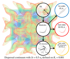
1 Introduction
Inertial droplets and/or particles in dispersed flows exhibit compression regions and intersecting trajectories which result in caustic formations (Crisanti et al. Reference Crisanti, Falcioni, Provenzale, Tanga and Vulpiani1992; Meneguz & Reeks Reference Meneguz and Reeks2011). Caustic formations (caustics) are zones of high concentration and their intensity is important to a great variety of environmental, biological, engineering and cosmological (Tomita & Den Reference Tomita and Den1986) applications. For example, the behaviour of micro-organisms is affected by the accumulation of nutrients (Vogel Reference Vogel1994) and the migration of sea organisms and coral colonies is governed by the formation of caustics created by sea currents (Serrano et al. Reference Serrano, Baums, Smith, Jones, Shearer and Baker2016). Sea currents and weather systems result in the local accumulation of pollutants, plastic debris (Lebreton et al. Reference Lebreton, Slat, Ferrari, Sainte-Rose, Aitken, Marthouse, Hajbane, Cunsolo, Schwarz and Levivier2018) and aerosols (Knight Reference Knight2012). Also, environmental pollution (Bell et al. Reference Bell, Dominici, Ebisu, Zeger and Samet2007), the impact of radioactive particles (Thomas & Martin Reference Thomas and Martin1986) and the potency of spray delivered medication (Rygg, Hindle & Longest Reference Rygg, Hindle and Longest2016), are strongly dependent on the formation of such accumulation regions (Sazhin Reference Sazhin2014). In internal combustion engines the vortical structures of the in-cylinder carrier phase flow field induce accumulation regions of the spray droplets during fuel injection, affecting the local stoichiometry of the mixture (Papoutsakis et al. Reference Papoutsakis, Sazhin, Begg, Danaila and Luddens2018b). Caustics in cumulus clouds have been reported to affect the patterns of rain (Ravichandran & Govindarajan Reference Ravichandran and Govindarajan2015) due to the sling effect of the vortical structures (Wilkinson et al. Reference Wilkinson, Mehlig, Östlund and Duncan2007).
In the general case, particles interact only due to collisions (Marble Reference Marble1970); for a diluted system of dispersed flows (Kasbaoui, Koch & Desjardins Reference Kasbaoui, Koch and Desjardins2019), however, interparticle collisions can be neglected (Williams Reference Williams1958; Bec Reference Bec2003), resulting in a pressureless continuum model (Tomita & Den Reference Tomita and Den1986; Kasbaoui et al. Reference Kasbaoui, Koch and Desjardins2019). The pressureless nature of dispersed flows allows the crossing of particle trajectories and results in caustic structures which are compression regions formed by the undulation of the dispersed phase. Standard Lagrangian approaches (LA) use a representative subset of the actual number of physical particles. Instances of caustics are singularities that cannot be captured accurately since they consist of a large concentration of particles focused in a small length scale, and demand a prohibitive number of representative Lagrangian particles to be described (Healy & Young Reference Healy and Young2005). In Papoutsakis et al. (Reference Papoutsakis, Rybdylova, Zaripov, Danaila, Osiptsov and Sazhin2018a) it was shown that the number density calculated with LA could not converge even for  $10^{6}$ representative particles per direction for a simple one-dimensional flow field.
The fully Lagrangian approach (standard FLA or Osiptsov method) (Osiptsov Reference Osiptsov1984, Reference Osiptsov2000) offers an efficient alternative by treating the particulate phase as a continuum. The FLA solves the particle number conservation equation in Lagrangian form along a single trajectory and provides the equations for the components of the Jacobi matrix of transformation from the Eulerian to the Lagrangian coordinates. This is essentially a method of characteristics and can deal with complex cases such as intersecting particle trajectories and caustics and presents unique properties in capturing the occurrence of accumulation regions. The FLA utilises the definition for the density  $\unicode[STIX]{x1D70C}$ for a deformed continuum, by introducing the Jacobian matrix determinant
 $|\boldsymbol{J}|$ (i.e.
 $\unicode[STIX]{x1D70C}_{0}=|\boldsymbol{J}|\unicode[STIX]{x1D70C}$) as it is used in solid mechanics (Healy & Young Reference Healy and Young2005). Although a dispersed phase consists of scattered individual entities, a dispersed continuum (DC) can be defined. This implies continuous fields for the particle number density and the particle velocity. Of course, the limit of the continuum assumption must be respected. Under the DC assumption, particles are transported while remaining attached to the Lagrangian DC, which is following the motion of the particles. Due to the absence of pressure in dispersed flows (in contrast to solid mechanics) the continuum can intersect itself, creating overlapping folds, and particle collisions may occur among particles that are attached to overlapping folds (Ravichandran & Govindarajan Reference Ravichandran and Govindarajan2015). The folds are areas of negative Jacobian, something that is not observed in continuum mechanics. It must be stressed here that even if pressure due to particle collisions is accounted for, dispersed flows do present intersecting trajectories. In the process of the creation of the folds for the DC, areas of zero Jacobian will emerge. The loci of zero Jacobian are characterised by infinite number density, thus, identifying caustic formations.
The efficiency and the modelling capabilities of the FLA in identifying the spatial structure of caustics was demonstrated in Healy & Young (Reference Healy and Young2005) and in Ijzermans et al. (Reference Ijzermans, Reeks, Meneguz, Picciotto and Soldati2009). The use of the FLA for the study of turbulent flows by Meneguz & Reeks (Reference Meneguz and Reeks2011) and by Picciotto et al. (Reference Picciotto, Marchioli, Reeks and Soldati2005) resulted in the identification and analysis of spatial structures of the dispersed phase distribution by introducing the moments of concentration. According to Picciotto et al. (Reference Picciotto, Marchioli, Reeks and Soldati2005) FLA has great potential for reductions in computational time compared with the standard Eulerian–Lagrangian approach and provides a sound mathematical framework for interpreting the physics of particulate flows.
However, the occurrence of singularities in the FLA hinders the applicability of the method. Singularities pose a serious controversy in the interpretation of the FLA results. In the literature, singularities are treated either by clipping large values of density (see Ducasse & Pumir Reference Ducasse and Pumir2009) or by introducing the concept of number density moments (i.e  $\overline{n^{a}}=\langle |\boldsymbol{J}|^{1-a}\rangle$ (Ijzermans, Meneguz & Reeks Reference Ijzermans, Meneguz and Reeks2010)) which was used for the analysis of spatial structures of the dispersed phase in turbulent flows. The zeroth moment has been used in Meneguz & Reeks (Reference Meneguz and Reeks2011) and in Ijzermans et al. (Reference Ijzermans, Meneguz and Reeks2010) for the evaluation of an averaged number density. This approach, however, cancels out the effect of the continuum deformation by multiplying the FLA density
 $1/|\boldsymbol{J}|$ by
 $|\boldsymbol{J}|$, and results in the transformation of the FLA to a standard Lagrangian approach. The averaged number density for higher moments gives non-physical values that reach to the order of
 $10^{10}$ (Ijzermans et al. Reference Ijzermans, Meneguz and Reeks2010; Meneguz & Reeks Reference Meneguz and Reeks2011). The actual values of these peaks are coincidental and are mostly related to the temporal resolution of the numerical integration during the instances of sign change of the Jacobian. A turbulent diffusion model was introduced for the ‘first-order’ FLA in Papoutsakis et al. (Reference Papoutsakis, Rybdylova, Zaripov, Danaila, Osiptsov and Sazhin2018a). The extended first-order FLA was implemented and assessed for direct numerical simulations (known as DNS) for Stokesian droplets in homogeneous isotropic turbulence (known as HIT) using the standard LA, and it was shown that the FLA singularities infect the spatially averaged result. Thus, it becomes essential that the FLA number density should be interpreted alongside with the spatial structure of the DC and must be connected to a length scale within a robust mathematical framework.
In this work we present an integrated framework that lifts the ambiguity of the FLA number density definition. We understand that because the FLA number density is defined for an infinitesimally small volume resulting in a pointwise density it results in singularities. Our approach is based on the observation that (a) the particulate phase and the DC are not identical concepts, instead the particles are sporadically attached to the DC at finite interparticle distances, and (b) the deformation of the DC cannot be captured by linear expressions; thus, it is necessary to account for the curvature of its structure. The model is based on representing the dispersed phase as a local approximation for the spatial DC structure, using the Jacobian and the Hessian of the transformation of the DC from the Lagrangian to the Eulerian coordinates. Choosing a first-order representation we obtain the standard FLA method, in a formulation that highlights the modelling capabilities and shortcomings of the standard FLA as a first-order approximation of the DC structure. In a second-order expression of the DC structure we obtain the derivation of an original second-order model, which provides the averaged FLA number density on a finite volume either by utilising the modelled second-order structure or by assuming a simplified one-dimensional structure on a primary direction.
Specifically, we present a model for the multidimensional structure of a dispersed phase based on the Jacobian and the Hessian of the transformation from the Lagrangian to the Eulerian coordinates. The Hessian and the Jacobian matrices are obtained by solving an initial value problem in multiple dimensions presented here, using a derivation that is in line with the Osiptsov method. Number density expressions are derived either from the three-dimensional structure or assuming a one-dimensional structure which is then projected along a primary direction. An algebraic model for the number density is derived and can be used for a reduced model of the number density and the DC structure by rotating the coordinate system along a primary direction. Thus, the derivation of all the elements needed for the application of the method to engineering problems is presented. The results inferred from the different approaches presented in this work are compared with the results stemming from the direct integration of individual particles. For the comparison of the two approaches (i.e. the LA and the FLA), the anisotropy of the length scales parallel and perpendicular to the caustic front are accounted for. In our study the proposed methodology is used for the investigation of caustic events for different Stokes numbers. Finally, the pressureless continuum assumption on a caustic is investigated by calculating the length scales of the average interparticle separation.
In § 2, a representation of the local DC structure based on the Taylor expansion of the DC coordinates is presented. This approach lays the foundations of the second-order FLA and also provides an insightful representation of the standard first-order FLA. In addition, the initial value problem for the calculation of the Hessian matrix in multidimensional problems is derived. In § 3 the local DC structure for a Stokesian dispersed phase convected by Taylor vortices is calculated using direct integration of a lattice of particles and is compared to the result from the first- and second-order representations. In § 4, the number density on a finite volume is defined. The results from the calculation of the number density, on multiple dimensions assuming a second-order one-dimensional DC structure based on the Hessian of the Lagrangian transformation (i.e. the curvature of the deformed DC), are also presented. In § 5 the effect of the Stokes number on the structure of caustic formations is investigated. Finally, in § 6 the findings from the implementation of the FLA for dispersed flows are discussed.
2 Second-order fully Lagrangian approach
The FLA provides a method to calculate the number density for a DC along the trajectory of a particle. A particle trajectory is the evolution of the position  $\boldsymbol{x}^{p}(t)$ of a particle with Lagrangian coordinate
 $(\boldsymbol{x}_{0}^{p},t)$ in time
 $t$. The vector
 $\boldsymbol{x}_{0}^{p}$ is the initial position of the particle at time
 $t=0$. The calculation of the number density in the FLA context is based on the transformation of an infinitesimal volume
 $V_{L}$ defined on the initial Lagrangian coordinates
 $\boldsymbol{x}_{0}^{p}$ to the deformed Lagrangian volume at
 $t$. The compression or expansion of
 $V_{L}$ is quantified by the Jacobian of the transformation defined as
 $\unicode[STIX]{x1D611}_{ij}=(\unicode[STIX]{x2202}x_{i}^{p}/\unicode[STIX]{x2202}x_{j,0}^{p})$, where
 $x_{j,0}^{p}$ is the Lagrangian coordinate and
 $x_{j}^{p}$ refers to the particle
 $p$ and is equivalent with the Eulerian coordinate
 $x_{j}$. In the FLA the number density
 $n^{p}$ along a trajectory, non-dimensionalised by the initial number density
 $n_{0}^{p}$, is
 $$\begin{eqnarray}n^{p}={\displaystyle \frac{1}{J}},\end{eqnarray}$$
where  $J$ is the determinant of the Jacobian matrix
 $\unicode[STIX]{x1D645}$. When
 $J$ tends to zero, the number density tends to infinity, thus signifying the occurrence of a caustic. The occurrence of singularities is due to the pointwise definition of the number density in the FLA framework
 $n^{p}=(\text{lim}_{V\rightarrow 0}N/V/n_{0}^{p})$. Since the particles are dispersed and are characterised by a minimum finite separation scale, this pointwise density corresponds to the DC structure rather than the particulate phase itself.
In order to investigate the integrability of this number density on a caustic, we need to focus on the Eulerian spatial structure of the DC. This can be revealed by representing the dispersed phase distribution in the vicinity of a particle trajectory using the coordinates of a particle  $\boldsymbol{x}^{p}(\boldsymbol{x}_{0}^{p}+\unicode[STIX]{x1D739},t)$ neighbouring to
 $\boldsymbol{x}^{p}(\boldsymbol{x}_{0}^{p},t)$, where the vector
 $\unicode[STIX]{x1D739}$ is the initial separation of the particles. Assuming a Taylor expansion for the distribution of the neighbours of
 $\boldsymbol{x}^{p}(\boldsymbol{x}_{0}^{p})$ at a time
 $t$, the DC structure can be represented as follows:
 $$\begin{eqnarray}\boldsymbol{x}^{p}(\boldsymbol{x}_{0}^{p}+\unicode[STIX]{x1D739})=\boldsymbol{x}^{p}(\boldsymbol{x}_{0}^{p})+{\displaystyle \frac{\unicode[STIX]{x2202}\boldsymbol{x}^{p}}{\unicode[STIX]{x2202}x_{j,0}^{p}}}\unicode[STIX]{x1D6FF}_{j}+{\displaystyle \frac{1}{2}}{\displaystyle \frac{\unicode[STIX]{x2202}^{2}\boldsymbol{x}^{p}}{\unicode[STIX]{x2202}x_{j,0}^{p}\unicode[STIX]{x2202}x_{k,0}^{p}}}\unicode[STIX]{x1D6FF}_{j}\unicode[STIX]{x1D6FF}_{k}+\cdots \,.\end{eqnarray}$$
Employing a linear expansion in three dimensions, the position  $\boldsymbol{x}+\unicode[STIX]{x1D750}$ of the particle
 $(\boldsymbol{x}_{0}+\unicode[STIX]{x1D739},t)$ in the vicinity of
 $(\boldsymbol{x}_{0},t)$ is expressed as
 $$\begin{eqnarray}\unicode[STIX]{x1D716}_{i}(\unicode[STIX]{x1D739})=\unicode[STIX]{x1D611}_{ij}\unicode[STIX]{x1D6FF}_{j},\end{eqnarray}$$
where  $\unicode[STIX]{x1D739}=\boldsymbol{x}_{0}-\boldsymbol{x}_{0}^{p}$ is the displacement vector of a particle at
 $t=0$ and
 $\unicode[STIX]{x1D750}=\boldsymbol{x}-\boldsymbol{x}^{p}$ is the displacement vector of the same particle at
 $t$. Vector indices
 $i,j$ correspond to vector components and summation is assumed among the repeated indices. It can be observed that the first-order spatial derivatives in (2.2) correspond to the Jacobian matrix; thus, (2.3) can be perceived as the expression of the DC structure in the standard FLA framework. In § 3 it will be shown that in the case of caustic formations (i.e.
 $J=0$), (2.3) results in an undefined structure where all particles collapse on a plane.
The linear representation of the dispersed phase degenerates when  $J=0$; however, this is not the case for the actual distribution of the particles. The equation (2.2) can be extended to account for a second-order description of the DC which provides the DC structure, even for small values of
 $J$, as follows:
 $$\begin{eqnarray}\unicode[STIX]{x1D716}_{i}(\unicode[STIX]{x1D6FF})=\unicode[STIX]{x1D611}_{ij}\unicode[STIX]{x1D6FF}_{j}+{\textstyle \frac{1}{2}}\unicode[STIX]{x1D60F}_{ijk}\unicode[STIX]{x1D6FF}_{j}\unicode[STIX]{x1D6FF}_{k},\end{eqnarray}$$
where  $\unicode[STIX]{x1D643}_{i}$ is a two-dimensional matrix, for each Cartesian coordinate
 $i$, and is defined as
 $\unicode[STIX]{x1D60F}_{ijk}=(\unicode[STIX]{x2202}^{2}x_{i}^{p}/\unicode[STIX]{x2202}x_{j,0}^{p}\unicode[STIX]{x2202}x_{k,0}^{p})$. Here,
 $\unicode[STIX]{x1D643}_{i}$ corresponds to the Hessian matrix of the transformation from the Eulerian to the Lagrangian coordinates.
For a particulate flow field with characteristic length  $L$ and a characteristic velocity
 $U$ we can define the non-dimensional carrier phase velocity field
 $\boldsymbol{U}$ and the induced particulate velocity
 $\boldsymbol{V}$. In the classical FLA, the Jacobian
 $\unicode[STIX]{x1D611}_{ij}=\unicode[STIX]{x2202}x_{i}^{p}/\unicode[STIX]{x2202}x_{j,0}^{p}$ is calculated by introducing the auxiliary variable
 $\unicode[STIX]{x1D714}_{ij}$, which is the time derivative of the Jacobian
 $$\begin{eqnarray}\unicode[STIX]{x1D714}_{ij}={\displaystyle \frac{\unicode[STIX]{x2202}\unicode[STIX]{x1D611}_{ij}}{\unicode[STIX]{x2202}t}}={\displaystyle \frac{\unicode[STIX]{x2202}}{\unicode[STIX]{x2202}t}}\left({\displaystyle \frac{\unicode[STIX]{x2202}x_{i}^{p}}{\unicode[STIX]{x2202}x_{j,0}^{p}}}\right)={\displaystyle \frac{\unicode[STIX]{x2202}V_{i}}{\unicode[STIX]{x2202}x_{j,0}^{p}}}.\end{eqnarray}$$
Although the calculation of the Jacobian can be extended to non-Stokesian particles (Papoutsakis et al. Reference Papoutsakis, Rybdylova, Zaripov, Danaila, Osiptsov and Sazhin2018a), we will assume a Stokesian drag force in our analysis. In this case the non-dimensional acceleration of the particles is  $\ddot{x}_{i}=\unicode[STIX]{x2202}V_{i}/\unicode[STIX]{x2202}t=1/St(U_{i}-V_{i})$, where
 $St=t_{p}/T$ is the Stokes number of the flow (Sazhin Reference Sazhin2014),
 $t_{p}$ is the particle relaxation time and
 $T=L/U$ is the characteristic time. Thus, following Osiptsov (Reference Osiptsov1984), the initial value problem for
 $\unicode[STIX]{x1D714}_{ij}$ is obtained as follows:
 $$\begin{eqnarray}{\displaystyle \frac{\unicode[STIX]{x2202}\unicode[STIX]{x1D714}_{ij}}{\unicode[STIX]{x2202}t}}={\displaystyle \frac{\unicode[STIX]{x2202}}{\unicode[STIX]{x2202}x_{j,0}^{p}}}\left({\displaystyle \frac{\unicode[STIX]{x2202}V_{i}}{\unicode[STIX]{x2202}t}}\right)={\displaystyle \frac{1}{St}}\left({\displaystyle \frac{\unicode[STIX]{x2202}x_{m}^{p}}{\unicode[STIX]{x2202}x_{j,0}^{p}}}{\displaystyle \frac{\unicode[STIX]{x2202}U_{i}}{\unicode[STIX]{x2202}x_{m}}}-{\displaystyle \frac{\unicode[STIX]{x2202}V_{i}}{\unicode[STIX]{x2202}x_{j,0}}}\right)={\displaystyle \frac{1}{St}}\left(J_{mj}{\displaystyle \frac{\unicode[STIX]{x2202}U_{i}}{\unicode[STIX]{x2202}x_{m}}}-\unicode[STIX]{x1D714}_{ij}\right),\end{eqnarray}$$
where addition is assumed among the terms with index  $m$. For the derivation of (2.6) the chain rule
 $\unicode[STIX]{x2202}(\cdot )/\unicode[STIX]{x2202}x_{i,0}=(\unicode[STIX]{x2202}(\cdot )/\unicode[STIX]{x2202}x_{i})\cdot (\unicode[STIX]{x2202}x_{i}^{p}/\unicode[STIX]{x2202}x_{i,0}^{p})$ is used with
 $x_{i}^{p}\equiv x_{i}$. The equation (2.6) is integrated using the initial condition
 $\unicode[STIX]{x1D714}_{ij}(t=0)=\unicode[STIX]{x2202}V_{i}/\unicode[STIX]{x2202}x_{j}|_{t=0}$ stemming from (2.5).
For the derivation of an expression for the Hessian  $\unicode[STIX]{x1D60F}_{ijk}$, needed for the second-order FLA in three dimensions, the auxiliary variable
 $\unicode[STIX]{x1D713}_{ijk}$ is introduced, defined as the time derivative of the Hessian
 $$\begin{eqnarray}\unicode[STIX]{x1D713}_{ijk}={\displaystyle \frac{\unicode[STIX]{x2202}\unicode[STIX]{x1D60F}_{ijk}}{\unicode[STIX]{x2202}t}}.\end{eqnarray}$$
The Hessian time rate  $\unicode[STIX]{x1D713}_{ijk}$ can be expressed as the spatial derivative of the rate of the Jacobian
 $\unicode[STIX]{x1D714}_{ij}$ over the Lagrangian coordinate
 $x_{k,0}^{p}$ as follows:
 $$\begin{eqnarray}{\displaystyle \frac{\unicode[STIX]{x2202}\unicode[STIX]{x1D713}_{ijk}}{\unicode[STIX]{x2202}t}}={\displaystyle \frac{\unicode[STIX]{x2202}}{\unicode[STIX]{x2202}t}}\left({\displaystyle \frac{\unicode[STIX]{x2202}\unicode[STIX]{x1D714}_{ij}}{\unicode[STIX]{x2202}x_{k,0}^{p}}}\right)={\displaystyle \frac{\unicode[STIX]{x2202}}{\unicode[STIX]{x2202}x_{k,0}^{p}}}\left({\displaystyle \frac{\unicode[STIX]{x2202}\unicode[STIX]{x1D714}_{ij}}{\unicode[STIX]{x2202}t}}\right)={\displaystyle \frac{\unicode[STIX]{x2202}}{\unicode[STIX]{x2202}x_{k,0}^{p}}}\left({\displaystyle \frac{1}{St}}\left(J_{mj}{\displaystyle \frac{\unicode[STIX]{x2202}U_{i}}{\unicode[STIX]{x2202}x_{m}}}-\unicode[STIX]{x1D714}_{ij}\right)\right).\end{eqnarray}$$
Using the chain rule as in (2.6) we finally obtain an expression for the Hessian time rate
 $$\begin{eqnarray}{\displaystyle \frac{\unicode[STIX]{x2202}\unicode[STIX]{x1D713}_{ijk}}{\unicode[STIX]{x2202}t}}={\displaystyle \frac{1}{St}}\left(H_{mjk}{\displaystyle \frac{\unicode[STIX]{x2202}U_{i}}{\unicode[STIX]{x2202}x_{m}}}+J_{mj}J_{nk}{\displaystyle \frac{\unicode[STIX]{x2202}^{2}U_{i}}{\unicode[STIX]{x2202}x_{m}\unicode[STIX]{x2202}x_{n}}}-\unicode[STIX]{x1D713}_{ijk}\right),\end{eqnarray}$$
where addition is assumed among the terms with indices  $m$ and
 $n$. For
 $t=0$, the Lagrangian derivative coincides with the Eulerian derivative; thus, the initial condition for
 $\unicode[STIX]{x1D713}$ is
 $\unicode[STIX]{x1D713}_{ijk}(t=0)=(\unicode[STIX]{x2202}^{2}V_{i}/\unicode[STIX]{x2202}x_{j}\unicode[STIX]{x2202}x_{k})$. Assuming that at
 $t=0$ the DC is not deformed, the expression
 $H(t=0)=0$ can be used as the initial value for
 $\unicode[STIX]{x1D60F}_{ijk}$.
The initial value problem for the calculation of the Hessian and the Jacobian under the second-order FLA concept as described by (2.5), (2.6), (2.7) and (2.9) can be summarised by the nonlinear first-order differential system
 $$\begin{eqnarray}{\displaystyle \frac{\unicode[STIX]{x2202}}{\unicode[STIX]{x2202}t}}\left[\begin{array}{@{}c@{}}\unicode[STIX]{x1D611}_{ij}\\ \unicode[STIX]{x1D714}_{ij}\\ \unicode[STIX]{x1D60F}_{ijk}\\ \unicode[STIX]{x1D713}_{ijk}\end{array}\right]=\left[\begin{array}{@{}c@{}}\unicode[STIX]{x1D714}_{ij}\\ {\displaystyle \frac{1}{St}}\left({\displaystyle \frac{\unicode[STIX]{x2202}U_{i}}{\unicode[STIX]{x2202}x_{m}}}J_{mj}-\unicode[STIX]{x1D714}_{ij}\right)\\ \unicode[STIX]{x1D713}_{ijk}\\ {\displaystyle \frac{1}{St}}\left(H_{mjk}{\displaystyle \frac{\unicode[STIX]{x2202}U_{i}}{\unicode[STIX]{x2202}x_{m}}}+J_{mj}J_{nk}{\displaystyle \frac{\unicode[STIX]{x2202}^{2}U_{i}}{\unicode[STIX]{x2202}x_{m}\unicode[STIX]{x2202}x_{n}}}-\unicode[STIX]{x1D713}_{ijk}\right)\end{array}\right]\;\left[\begin{array}{@{}c@{}}\unicode[STIX]{x1D611}_{ij}\\ \unicode[STIX]{x1D714}_{ij}\\ \unicode[STIX]{x1D60F}_{ijk}\\ \unicode[STIX]{x1D713}_{ijk}\end{array}\right]_{t=0}=\left[\begin{array}{@{}c@{}}\unicode[STIX]{x1D6FF}_{i,j}\\ {\displaystyle \frac{\unicode[STIX]{x2202}V_{i}}{\unicode[STIX]{x2202}x_{j}}}\\ 0\\ {\displaystyle \frac{\unicode[STIX]{x2202}^{2}V_{i}}{\unicode[STIX]{x2202}x_{j}\unicode[STIX]{x2202}x_{k}}}\end{array}\right],\end{eqnarray}$$
where addition is assumed among the terms  $m=1\ldots 3$ and
 $n=1\ldots 3$. The system of (2.10) is integrated with an appropriate numerical method (e.g. Runge–Kutta) and provides the entries of the Jacobian and the Hessian matrices along a particle trajectory.
From (2.10) it can be inferred that for a linear converging flow field with  $U(y)=-y$,
 $\unicode[STIX]{x2202}^{2}U/\unicode[STIX]{x2202}x^{2}=0$, the Hessian is zero and at the focal point
 $y=0$ the number density will be genuinely infinite (Morse point) as all particles will meet at the same location. As the curvature of the carrier phase field becomes non-zero, the Hessian will be generally non-zero (
 $H\neq 0$) and the number density would be finite.
(a) Distribution of particles at  $t=0.4$. (b) Solid black line, the trajectory of the reference particle from
 $t=0$ to
 $t>0.45$ as calculated by direct integration of the particle equation of motion assuming Stokes particles; black dots, distribution of the neighbouring particles calculated by direct integration of the particle equation of motion; red lines, particle distribution inferred from the second-order description of the DC structure; black lines, particle distribution inferred from the first-order description of the DC structure. The particle distributions are shown at regular intervals
 $t=0.00,0.05,0.10,0.15,\ldots ,0.45$ and at
 $t=0.1655$. Instance
 $t=0.1655$ corresponds to a caustic formation. The vector field represents the carrier phase velocity field.

3 Second-order structure of a Stokesian dispersed phase in a periodic two-dimensional array of Taylor vortices
In this section we present the result from a kinematic simulation (KS) (see Monchaux, Bourgoin & Cartellier (Reference Monchaux, Bourgoin and Cartellier2012)) of a DC that conveys in a carrier phase flow field consisting of a periodic distribution of two-dimensional stationary Taylor vortices. Similar synthetic flow fields have been used in the analysis of Crisanti et al. (Reference Crisanti, Falcioni, Provenzale, Tanga and Vulpiani1992). The dispersed phase consists of  $500\times 500$ individual particles with Stokes number
 $St=0.1$. Initially, the particles are uniformly distributed in a square with size
 $L$. The carrier phase flow field
 $\boldsymbol{U}=(U_{1},U_{2})$ is an incompressible synthetic flow field defined by the analytical expressions
 $$\begin{eqnarray}U_{1}(x,y)=U_{0}\cos (2\unicode[STIX]{x03C0}nx)\sin (2\unicode[STIX]{x03C0}ny)\quad \text{and}\quad U_{2}(x,y)=-U_{0}\sin (2\unicode[STIX]{x03C0}nx)\cos (2\unicode[STIX]{x03C0}ny),\end{eqnarray}$$
where  $x$ and
 $y$ are the dimensionless coordinates, normalised by
 $L$. The velocity amplitude
 $U_{0}$, non-dimensionalised by
 $U$, is equal to
 $U_{0}=5$ and the wavenumber is
 $n=2$. The result of the particles distribution at time
 $t=0.4$ as calculated by integrating the equation of motion
 $\ddot{\boldsymbol{x}}^{p}=(\boldsymbol{U}-\boldsymbol{V})/St$, is shown in figure 1(a). Equation (3.1) provides the exact values of the velocity field and its spatial derivatives at any point of the Eulerian domain, needed for the integration of the initial value problem described by (2.10), as well as for the solution of the equation of motion. The equation of motion and the initial value problem (2.10) are both integrated using a fourth-order Runge–Kutta method.
In figure 1(a) the position of each particle is shown by transparent black-coloured circles and the particle agglomeration is identified by the dark filaments shown in this figure. The trajectory of a single particle initially located at  $(-0.05,0.1)$ is shown in figure 1(b). The distribution of
 $80$ particles neighbouring the reference particle and arranged in a rectilinear lattice of
 $9\times 9$ particles with an initial separation
 $|\unicode[STIX]{x1D739}|=0.0005$ is also shown in figure 1(b). Their trajectories are calculated by direct integration and they are presented as black dots at regular intervals. The black and red lines in figure 1(b) represent the local DC structure as calculated by (2.3) and (2.4) which correspond to the first- and second-order representation of the DC structure, using the initial separation vector
 $|\unicode[STIX]{x1D739}|$ for each neighbouring particle. The components of the Jacobian and the Hessian matrices needed by (2.3) and (2.4) are calculated by the initial value problem (2.10), derived in the previous section.
Distribution of individual particles compared to the DC structure calculated by different models. The plots are presented on the coordinate system (shown by the thin black line crosshair) that is attached to the reference particle. Black dots, distribution of particles neighbouring to the reference trajectory; red grid lines, particle distribution inferred from the second-order description of the DC structure; black grid lines, particle distribution inferred from the first-order description of the DC structure; orange grid lines, particle distribution inferred from the first-order one-dimensional description of the DC structure. Panel (b) corresponds to a caustic formation, where the lattice that corresponds to the first-order representation (shown with the black grid lines) has degenerated to a straight line.

4 Calculation of the particle number density
In this section, a method for calculating a number density defined at a finite length scale is presented. This number density is calculated from the first- and second-order model for the DC structure. An analytical model for the number density, assuming a one-dimensional second-order representation of the DC, is also derived. In figure 2(a–d) we focus on the dispersed phase for four instances. From figure 2(a–d) and from figure 1(b) it can be inferred that the second-order FLA can provide a satisfactory approximation of the DC structure even at significant distances from the reference trajectory. The method not only captures the compression of the DC but also resolves the complex non-isotropic DC structure even when this collapses to a caustic filament (see figure 2b).
In conjunction with the pointwise density  $n^{p}$, a number density
 $\hat{n}^{p}$ defined at a finite length scale can be inferred from the DC structure calculated by each one of the three methods shown in figure 2, as follows:
 $$\begin{eqnarray}\hat{n}^{p}={\displaystyle \frac{1}{S_{t}}},\end{eqnarray}$$
where  $\hat{n}^{p}$ has been normalised by the initial number density
 $n_{0}^{p}$, and
 $S_{t}$ is the surface of the lattice defined by the eight particles closest to the reference particle
 $p$ at
 $t$ normalised by the initial surface of the lattice
 $S_{0}$. The number density
 $\hat{n}^{p}$ in (4.1) is defined at a finite length scale
 $\unicode[STIX]{x1D6E5}\sim \sqrt{S_{t}}$. Figure 2(b) corresponds to the instance
 $t=0.1655$, for which the particles agglomerate to a caustic. In figure 2(b) it can be observed that the first-order structure as provided by (2.3) and indicated by the black line mesh, collapses to a single line with
 $S_{t}=0$, since
 $J_{11}J_{22}-J_{12}J_{21}=0$. This results in an infinite number density
 $n=1/J$. The rationale behind the occurrence of infinite number densities in the standard FLA lies in the fact that the first-order approach provides a pointwise number density (i.e. the number density that corresponds to an infinitesimally small volume) and is based on the local DC deformation. This behaviour is non-physical because number density should be defined for a finite length scale. The particulate phase is dispersed; thus, the definition of a pointwise definition breaches the continuity assumption.
For the derivation of an analytical model for a number density defined at a finite length scale, we can assume a simplified one-dimensional second-order DC structure for a caustic formation. This assumption can be based on the observation that these formations appear as filaments with a one-dimensional structure along a preferential direction (see figure 1). A coordinate system  $\unicode[STIX]{x1D6FF},\unicode[STIX]{x1D716}$ attached to the reference particle and perpendicular to the filament can be chosen so that
 $J$ and
 $H$ are both positive (see figure 3). Thus a one-dimensional DC structure can be expressed as
 $\unicode[STIX]{x1D716}(\unicode[STIX]{x1D6FF})=J\unicode[STIX]{x1D6FF}+0.5H\unicode[STIX]{x1D6FF}^{2}$ (or as
 $\unicode[STIX]{x1D6FF}(\unicode[STIX]{x1D716})=(-J+\sqrt{J^{2}+2H\unicode[STIX]{x1D716}}/H)$, where the binomial root closer to the reference point is chosen).
One-dimensional structure of the DC: for the scenario  $\boldsymbol{A}$,
 $J^{2}-2HR_{\unicode[STIX]{x1D716}}>0$; and for the scenario
 $\boldsymbol{B}$,
 $J^{2}-2HR_{\unicode[STIX]{x1D716}}<0$, when the caustic fold occurs within the filtering volume.

The solid line in figure 3 depicts the schematic representation of a one-dimensional DC. The DC is presented in terms of the Lagrangian  $x_{0}$ and Eulerian
 $x$ coordinate. In the specific example the DC has folded; thus, it is multiply defined for a part of the Eulerian field. The local coordinate
 $\unicode[STIX]{x1D716}$ corresponds to the Eulerian coordinate
 $\boldsymbol{x}$ and the local coordinate
 $\unicode[STIX]{x1D6FF}$ corresponds to the Lagrangian coordinate
 $\boldsymbol{x}_{0}$. The averaged pointwise number density
 $1/J=\text{d}\unicode[STIX]{x1D6FF}/\text{d}\unicode[STIX]{x1D716}$ for an interval
 $[-R_{\unicode[STIX]{x1D716}},R_{\unicode[STIX]{x1D716}}]$ with length
 $L=2R_{\unicode[STIX]{x1D716}}$ at the proximity of the point
 $\boldsymbol{A}$ shown in figure 3 (scenario
 $\boldsymbol{A}$) is
 $$\begin{eqnarray}\hat{n}^{p}={\displaystyle \frac{1}{2R_{\unicode[STIX]{x1D716}}}}\int _{-R_{\unicode[STIX]{x1D716}}}^{R_{\unicode[STIX]{x1D716}}}{\displaystyle \frac{\text{d}\unicode[STIX]{x1D6FF}}{\text{d}\unicode[STIX]{x1D716}}}\,\text{d}\unicode[STIX]{x1D716}={\displaystyle \frac{\left|\unicode[STIX]{x1D6FF}(R_{\unicode[STIX]{x1D716}})-\unicode[STIX]{x1D6FF}(-R_{\unicode[STIX]{x1D716}})\right|}{2R_{\unicode[STIX]{x1D716}}}},\end{eqnarray}$$
where  $\unicode[STIX]{x1D6FF}(\pm R_{\unicode[STIX]{x1D716}})=(-J+\sqrt{J^{2}\pm 2HR_{\unicode[STIX]{x1D716}}})/H$.
For the lower bound of the interval  $[-R_{\unicode[STIX]{x1D716}},R_{\unicode[STIX]{x1D716}}]$ (i.e.
 $\unicode[STIX]{x1D716}=-R_{\unicode[STIX]{x1D716}}$) the equation
 $\unicode[STIX]{x1D716}(\unicode[STIX]{x1D6FF})=-R_{\unicode[STIX]{x1D716}}$ will not have a root if
 $J^{2}<2HR_{\unicode[STIX]{x1D716}}$ (see scenario
 $\boldsymbol{B}$, figure 3a). This scenario occurs when the caustic occurs within the Eulerian interval
 $[-R_{\unicode[STIX]{x1D716}},R_{\unicode[STIX]{x1D716}}]$ and there is a minimum
 $\unicode[STIX]{x1D716}=J\unicode[STIX]{x1D6FF}+0.5H\unicode[STIX]{x1D6FF}^{2}$,
 $\unicode[STIX]{x1D716}_{min}=-(J^{2}/2H)>-R_{\unicode[STIX]{x1D716}}$ for
 $\unicode[STIX]{x1D6FF}_{min}=\unicode[STIX]{x1D6FF}(\unicode[STIX]{x1D716}_{min})=-J/H$. In this case the integration is done along the interval
 $[\unicode[STIX]{x1D716}_{min},R_{\unicode[STIX]{x1D716}}]$, with length
 $L_{1}=R_{\unicode[STIX]{x1D716}}-\unicode[STIX]{x1D716}_{min}$ for the first branch of the caustic formation and along an interval with length
 $L_{2}$ on the second branch of the caustic. By ensuring that
 $L=L_{1}+L_{2}=2R_{\unicode[STIX]{x1D716}}$ for the two branches, the interval for the second branch is
 $[\unicode[STIX]{x1D716}_{min},R_{\unicode[STIX]{x1D716}}+2\unicode[STIX]{x1D716}_{min}]$. Thus, the averaged number density for scenario
 $\boldsymbol{B}$ is
 $$\begin{eqnarray}\hat{n}^{p}={\displaystyle \frac{1}{2R_{\unicode[STIX]{x1D716}}}}\int _{\unicode[STIX]{x1D716}_{min}}^{R_{\unicode[STIX]{x1D716}}}{\displaystyle \frac{\text{d}\unicode[STIX]{x1D6FF}}{\text{d}\unicode[STIX]{x1D716}}}\,\text{d}\unicode[STIX]{x1D716}+{\displaystyle \frac{1}{2R_{\unicode[STIX]{x1D716}}}}\int _{\unicode[STIX]{x1D716}_{min}}^{R_{\unicode[STIX]{x1D716}}+2\unicode[STIX]{x1D716}_{min}}{\displaystyle \frac{\text{d}\unicode[STIX]{x1D6FF}}{\text{d}\unicode[STIX]{x1D716}}}\,\text{d}\unicode[STIX]{x1D716}={\displaystyle \frac{\left|\unicode[STIX]{x1D6FF}(R_{\unicode[STIX]{x1D716}})-\unicode[STIX]{x1D6FF}_{min}\right|+\left|\unicode[STIX]{x1D6FF}(R_{\unicode[STIX]{x1D716}}+2\unicode[STIX]{x1D716}_{min})-\unicode[STIX]{x1D6FF}_{min}\right|}{2R_{\unicode[STIX]{x1D716}}}}.\end{eqnarray}$$
Finally, introducing the roots  $\unicode[STIX]{x1D6FF}(\pm R_{\unicode[STIX]{x1D716}})=(-J+\sqrt{J^{2}\pm 2HR_{\unicode[STIX]{x1D716}}})/H$ in (4.2) for the scenario
 $\boldsymbol{A}$, and the roots
 $\unicode[STIX]{x1D6FF}(R_{\unicode[STIX]{x1D716}})=(-J+\sqrt{J^{2}+2HR_{\unicode[STIX]{x1D716}}})/H$,
 $\unicode[STIX]{x1D6FF}(\unicode[STIX]{x1D716}_{min})=-J/H$ and
 $\unicode[STIX]{x1D6FF}(R_{\unicode[STIX]{x1D716}}+2\unicode[STIX]{x1D716})=(-J+\sqrt{2HR_{\unicode[STIX]{x1D716}}-J^{2}})/H$ in (4.3) for the scenario
 $\boldsymbol{B}$,
 $\hat{n}^{p}$ averaged on a characteristic length scale
 $2R_{\unicode[STIX]{x1D716}}$ is
 $$\begin{eqnarray}\hat{n}^{p}=\left\{\begin{array}{@{}ll@{}}{\displaystyle \frac{2}{\sqrt{J^{2}+2HR_{\unicode[STIX]{x1D716}}}+\sqrt{J^{2}-2HR_{\unicode[STIX]{x1D716}}}}}\quad & \text{if }J^{2}-2HR_{\unicode[STIX]{x1D716}}>0\\[10.0pt] {\displaystyle \frac{\sqrt{J^{2}+2HR_{\unicode[STIX]{x1D716}}}+\sqrt{-J^{2}+2HR_{\unicode[STIX]{x1D716}}}}{2R_{\unicode[STIX]{x1D716}}H}}\quad & \text{if }J^{2}-2HR_{\unicode[STIX]{x1D716}}<0.\end{array}\right.\end{eqnarray}$$
For  $J^{2}\gg 2HR_{\unicode[STIX]{x1D716}}$, the above expression simplifies to the classical FLA expression
 $\hat{n}^{p}=1/J$.
For the calculation of a scalar magnitude  $\boldsymbol{H}$ for the Hessian, along the primary direction of a caustic filament from
 $\unicode[STIX]{x1D60F}_{ijk}$, the angle
 $\unicode[STIX]{x1D703}$ between the coordinate systems that are attached to the fold (i.e.
 $(\unicode[STIX]{x1D702},\unicode[STIX]{x1D701})$ and
 $(\unicode[STIX]{x1D702}_{0},\unicode[STIX]{x1D701}_{0})$) in relation to the global coordinates
 $(x,y)$ and
 $(x_{0},y_{0})$ is assumed. The transformation between the two systems for both the initial and the current positions is written as follows:
 $$\begin{eqnarray}\displaystyle & \displaystyle (\unicode[STIX]{x1D702},\unicode[STIX]{x1D702}_{0})=(x,x_{0})\cos \unicode[STIX]{x1D703}+(y,y_{0})\sin \unicode[STIX]{x1D703},(\unicode[STIX]{x1D701},\unicode[STIX]{x1D701}_{0})=-(x,x_{0})\sin \unicode[STIX]{x1D703}+(y,y_{0})\cos \unicode[STIX]{x1D703}, & \displaystyle\end{eqnarray}$$
 $$\begin{eqnarray}\displaystyle & \displaystyle (x,x_{0})=(\unicode[STIX]{x1D702},\unicode[STIX]{x1D702}_{0})\cos \unicode[STIX]{x1D703}-(\unicode[STIX]{x1D701},\unicode[STIX]{x1D701}_{0})\sin \unicode[STIX]{x1D703},\quad (y,y_{0})=(\unicode[STIX]{x1D702},\unicode[STIX]{x1D702}_{0})\sin \unicode[STIX]{x1D703}+(\unicode[STIX]{x1D701},\unicode[STIX]{x1D701}_{0})\cos \unicode[STIX]{x1D703}. & \displaystyle\end{eqnarray}$$
Based on the assumption of the one-dimensional structure of the caustic filament, the curvature of the DC on the  $\unicode[STIX]{x1D701}$ direction can be ignored and a Hessian magnitude
 $\boldsymbol{H}$ on the direction
 $\unicode[STIX]{x1D701}$ can be defined as
 $\boldsymbol{H}=(\unicode[STIX]{x2202}^{2}\unicode[STIX]{x1D702}/\unicode[STIX]{x2202}\unicode[STIX]{x1D702}_{0}^{2})$. In order to evaluate the second derivative, we start from the first derivative which can be written as follows:
 $$\begin{eqnarray}{\displaystyle \frac{\unicode[STIX]{x2202}\unicode[STIX]{x1D702}}{\unicode[STIX]{x2202}\unicode[STIX]{x1D702}_{0}}}={\displaystyle \frac{\unicode[STIX]{x2202}\unicode[STIX]{x1D702}}{\unicode[STIX]{x2202}x_{0}}}{\displaystyle \frac{\unicode[STIX]{x2202}x_{0}}{\unicode[STIX]{x2202}\unicode[STIX]{x1D702}_{0}}}+{\displaystyle \frac{\unicode[STIX]{x2202}\unicode[STIX]{x1D702}}{\unicode[STIX]{x2202}y_{0}}}{\displaystyle \frac{\unicode[STIX]{x2202}y_{0}}{\unicode[STIX]{x2202}\unicode[STIX]{x1D702}_{0}}}={\displaystyle \frac{\unicode[STIX]{x2202}x}{\unicode[STIX]{x2202}x_{0}}}\cos ^{2}\unicode[STIX]{x1D703}+{\displaystyle \frac{\unicode[STIX]{x2202}y}{\unicode[STIX]{x2202}x_{0}}}\sin \unicode[STIX]{x1D703}\cos \unicode[STIX]{x1D703}+{\displaystyle \frac{\unicode[STIX]{x2202}x}{\unicode[STIX]{x2202}y_{0}}}\sin \unicode[STIX]{x1D703}\cos \unicode[STIX]{x1D703}+{\displaystyle \frac{\unicode[STIX]{x2202}y}{\unicode[STIX]{x2202}y_{0}}}\sin ^{2}\unicode[STIX]{x1D703}.\end{eqnarray}$$
This result is obtained using the transformation equations (4.5) for  $\unicode[STIX]{x1D702}$ and
 $\unicode[STIX]{x1D701}$ in terms of
 $x$ and
 $y$ and the partial derivatives of the Lagrangian coordinates, deduced from (4.6) (i.e.
 $\unicode[STIX]{x2202}x_{0}/\unicode[STIX]{x2202}\unicode[STIX]{x1D702}_{0}=\cos \unicode[STIX]{x1D703}$ and
 $\unicode[STIX]{x2202}y_{0}/\unicode[STIX]{x2202}\unicode[STIX]{x1D702}_{0}=\sin \unicode[STIX]{x1D703}$). The second derivative is obtained by differentiating (4.7) on
 $\unicode[STIX]{x1D702}_{0}$ using the expressions
 $\unicode[STIX]{x2202}x_{0}/\unicode[STIX]{x2202}\unicode[STIX]{x1D702}_{0}=\cos \unicode[STIX]{x1D703}$ and
 $\unicode[STIX]{x2202}y_{0}/\unicode[STIX]{x2202}\unicode[STIX]{x1D702}_{0}=\sin \unicode[STIX]{x1D703}$, and also the following evaluations of the chain rule:
 $$\begin{eqnarray}\left.\begin{array}{@{}c@{}}\displaystyle {\displaystyle \frac{\unicode[STIX]{x2202}}{\unicode[STIX]{x2202}\unicode[STIX]{x1D702}_{0}}}\left({\displaystyle \frac{\unicode[STIX]{x2202}x}{\unicode[STIX]{x2202}x_{0}}}\right)={\displaystyle \frac{\unicode[STIX]{x2202}^{2}x}{\unicode[STIX]{x2202}x_{0}\unicode[STIX]{x2202}x_{0}}}{\displaystyle \frac{\unicode[STIX]{x2202}x_{0}}{\unicode[STIX]{x2202}\unicode[STIX]{x1D702}_{0}}}+{\displaystyle \frac{\unicode[STIX]{x2202}^{2}x}{\unicode[STIX]{x2202}y_{0}\unicode[STIX]{x2202}x_{0}}}{\displaystyle \frac{\unicode[STIX]{x2202}y_{0}}{\unicode[STIX]{x2202}\unicode[STIX]{x1D702}_{0}}},\\[10.0pt] \displaystyle {\displaystyle \frac{\unicode[STIX]{x2202}}{\unicode[STIX]{x2202}\unicode[STIX]{x1D702}_{0}}}\left({\displaystyle \frac{\unicode[STIX]{x2202}y}{\unicode[STIX]{x2202}x_{0}}}\right)={\displaystyle \frac{\unicode[STIX]{x2202}^{2}y}{\unicode[STIX]{x2202}x_{0}\unicode[STIX]{x2202}x_{0}}}{\displaystyle \frac{\unicode[STIX]{x2202}x_{0}}{\unicode[STIX]{x2202}\unicode[STIX]{x1D702}_{0}}}+{\displaystyle \frac{\unicode[STIX]{x2202}^{2}y}{\unicode[STIX]{x2202}y_{0}\unicode[STIX]{x2202}x_{0}}}{\displaystyle \frac{\unicode[STIX]{x2202}y_{0}}{\unicode[STIX]{x2202}\unicode[STIX]{x1D702}_{0}}},\\[10.0pt] \displaystyle {\displaystyle \frac{\unicode[STIX]{x2202}}{\unicode[STIX]{x2202}\unicode[STIX]{x1D702}_{0}}}\left({\displaystyle \frac{\unicode[STIX]{x2202}x}{\unicode[STIX]{x2202}y_{0}}}\right)={\displaystyle \frac{\unicode[STIX]{x2202}^{2}x}{\unicode[STIX]{x2202}x_{0}\unicode[STIX]{x2202}y_{0}}}{\displaystyle \frac{\unicode[STIX]{x2202}x_{0}}{\unicode[STIX]{x2202}\unicode[STIX]{x1D702}_{0}}}+{\displaystyle \frac{\unicode[STIX]{x2202}^{2}x}{\unicode[STIX]{x2202}y_{0}\unicode[STIX]{x2202}y_{0}}}{\displaystyle \frac{\unicode[STIX]{x2202}y_{0}}{\unicode[STIX]{x2202}\unicode[STIX]{x1D702}_{0}}},\\[10.0pt] \displaystyle {\displaystyle \frac{\unicode[STIX]{x2202}}{\unicode[STIX]{x2202}\unicode[STIX]{x1D702}_{0}}}\left({\displaystyle \frac{\unicode[STIX]{x2202}y}{\unicode[STIX]{x2202}y_{0}}}\right)={\displaystyle \frac{\unicode[STIX]{x2202}^{2}y}{\unicode[STIX]{x2202}x_{0}\unicode[STIX]{x2202}y_{0}}}{\displaystyle \frac{\unicode[STIX]{x2202}x_{0}}{\unicode[STIX]{x2202}\unicode[STIX]{x1D702}_{0}}}+{\displaystyle \frac{\unicode[STIX]{x2202}^{2}y}{\unicode[STIX]{x2202}y_{0}\unicode[STIX]{x2202}y_{0}}}{\displaystyle \frac{\unicode[STIX]{x2202}y_{0}}{\unicode[STIX]{x2202}\unicode[STIX]{x1D702}_{0}}}.\end{array}\right\}\end{eqnarray}$$
The second derivative  $\boldsymbol{H}=(\unicode[STIX]{x2202}^{2}\unicode[STIX]{x1D702}/\unicode[STIX]{x2202}\unicode[STIX]{x1D702}_{0}^{2})$ can be obtained from (4.7) as follows:
 $$\begin{eqnarray}\displaystyle \boldsymbol{H} & = & \displaystyle H_{111}\cos ^{3}\unicode[STIX]{x1D703}+H_{121}\cos ^{2}\unicode[STIX]{x1D703}\sin \unicode[STIX]{x1D703}+H_{211}\cos ^{2}\unicode[STIX]{x1D703}\sin \unicode[STIX]{x1D703}+H_{221}\cos \unicode[STIX]{x1D703}\sin ^{2}\unicode[STIX]{x1D703}\nonumber\\ \displaystyle & & \displaystyle +\,H_{112}\cos ^{2}\unicode[STIX]{x1D703}\sin \unicode[STIX]{x1D703}+H_{122}\cos \unicode[STIX]{x1D703}\sin ^{2}\unicode[STIX]{x1D703}+H_{212}\cos \unicode[STIX]{x1D703}\sin ^{2}\unicode[STIX]{x1D703}+H_{222}\sin ^{3}\unicode[STIX]{x1D703}.\end{eqnarray}$$
The primary direction of the fold is calculated by finding the  $\unicode[STIX]{x1D703}\in [0:2\unicode[STIX]{x03C0}]$ that maximises
 $\boldsymbol{H}$ in (4.9). This maximum value
 $\boldsymbol{H}$ is used for the evaluation of the number density for a finite volume with radius
 $R_{\unicode[STIX]{x1D716}}$ as dictated by (4.4). The result of this analysis for
 $\hat{n}^{p}$ at the instance
 $t=0.4$ and
 $R_{\unicode[STIX]{x1D716}}=0.001$ is shown in figure 4. It can be observed that this method provides a finite value for
 $\hat{n}^{p}$ and the loci of number density maxima corresponds to the caustic formations shown in figure 1.
The orange grid lines in figure 2(a–d) represent the DC structure as described by the second-order FLA, assuming this one-dimensional structure, that accounts for the DC curvature along the primary direction only. The Taylor expansion of the Eulerian coordinates  $(\unicode[STIX]{x1D702},\unicode[STIX]{x1D701})$, expressed in terms of the Lagrangian coordinates
 $(\unicode[STIX]{x1D702}_{0},\unicode[STIX]{x1D701}_{0})$, across the primary direction
 $\unicode[STIX]{x1D703}$, is
 $$\begin{eqnarray}\unicode[STIX]{x1D702}=J_{1,1}\unicode[STIX]{x1D702}_{0}+J_{1,2}\unicode[STIX]{x1D701}_{0}+0.5\boldsymbol{H}\unicode[STIX]{x1D702}_{0}^{2},\quad \unicode[STIX]{x1D701}=J_{2,1}\unicode[STIX]{x1D702}_{0}+J_{2,2}\unicode[STIX]{x1D701}_{0},\end{eqnarray}$$
where the second derivatives in the  $\unicode[STIX]{x1D701}$ direction are assumed to be equal to zero, i.e.
 $(\unicode[STIX]{x2202}^{2}/\unicode[STIX]{x2202}\unicode[STIX]{x1D701}_{0}^{2})=0$, and also
 $(\unicode[STIX]{x2202}^{2}\unicode[STIX]{x1D701}/\unicode[STIX]{x2202}\unicode[STIX]{x1D702}_{0}^{2})=0$. Rotating the above expression by the principal direction angle
 $\unicode[STIX]{x1D703}$, the DC structure on the
 $x,y$ plane (
 $\unicode[STIX]{x1D716}_{1}=x-x^{p}$ and
 $\unicode[STIX]{x1D716}_{2}=y-y^{p}$) is expressed as
 $$\begin{eqnarray}x-x^{p}=J_{1,1}\unicode[STIX]{x1D6FF}_{1}+J_{1,2}\unicode[STIX]{x1D6FF}_{2}+0.5\boldsymbol{H}\unicode[STIX]{x1D6FF}_{1}^{2}\cos ^{3}\unicode[STIX]{x1D703}+\boldsymbol{H}\cos ^{2}\unicode[STIX]{x1D703}\sin \unicode[STIX]{x1D703}\unicode[STIX]{x1D6FF}_{1}\unicode[STIX]{x1D6FF}_{2}+0.5\boldsymbol{H}\cos \unicode[STIX]{x1D703}\sin ^{2}\unicode[STIX]{x1D703}\unicode[STIX]{x1D6FF}_{2}^{2}\end{eqnarray}$$
and
 $$\begin{eqnarray}y-y^{p}=J_{2,1}\unicode[STIX]{x1D6FF}_{1}+J_{2,2}\unicode[STIX]{x1D6FF}_{2}+0.5\boldsymbol{H}\unicode[STIX]{x1D6FF}_{1}^{2}\cos ^{2}\unicode[STIX]{x1D703}\sin \unicode[STIX]{x1D703}+\boldsymbol{H}\cos \unicode[STIX]{x1D703}\sin ^{2}\unicode[STIX]{x1D703}\unicode[STIX]{x1D6FF}_{1}\unicode[STIX]{x1D6FF}_{2}+0.5\boldsymbol{H}\sin ^{3}\unicode[STIX]{x1D703}\unicode[STIX]{x1D6FF}_{2}^{2},\end{eqnarray}$$
where  $\unicode[STIX]{x1D6FF}_{1}=x_{0}-x_{0}^{p}$ and
 $\unicode[STIX]{x1D6FF}_{2}=y_{0}-y_{0}^{p}$.
In figure 5 we present a comparison of the number densities for the reference particle  $(-0.05,0.1)$ calculated using the standard FLA (see (2.1)), the second-order FLA (4.1) and the second-order FLA using a one-dimensional structure for the DC (see (4.4) and (4.9)), compared to the result inferred from the direct numerical integration of particle trajectories using (4.1).
In order to calculate all densities from the various models and compare them to the LA result, at a consistent length scale, the analytical model described by (4.4) is evaluated at a length scale  $R_{\unicode[STIX]{x1D716}}$ which is inferred from the LA simulation. The
 $R_{\unicode[STIX]{x1D716}}$ shown in figure 3 corresponds to the length scale of the caustic formation across the agglomeration front. The deformed DC on a caustic is a strongly anisotropic filament and is characterised by a maximum and a minimum length, namely
 $R_{max}$ and
 $R_{min}$, respectively. An estimate for the thickness of this caustic filament
 $R_{\unicode[STIX]{x1D716}}$ can be obtained from
 $R_{min}$. Given that we know the surface of the caustic
 $S_{t}$ the minimum length scale that corresponds to the deformed caustic can be calculated from
 $R_{max}$ as
 $R_{min}=S_{t}/(4R_{max})$. Thus an estimate for
 $R_{\unicode[STIX]{x1D716}}$ is
 $R_{\unicode[STIX]{x1D716}}=S_{t}/(4R_{max})$.
Instance  $t=0.4$, represented as a deformed DC. The gradient of the surface identifies the caustic formations and its curvature is related to the intensity of the caustics. The surface is coloured by
 $\hat{n}^{p}$, with
 $R_{\unicode[STIX]{x1D716}}=0.001$. Here,
 $St=0.1$.

As it can be inferred from figure 5(a), all approaches predict the number density as calculated by the direct integration of a dense cloud of particle trajectories using the standard LA for almost the whole interval of the simulation. At the instance  $t\sim 0.1655$, however, and for a duration of
 $\unicode[STIX]{x0394}t\sim 0.001$, the reference particle goes through a caustic. The performance of the approaches presented close to the caustic is shown in detail in figure 5(b). As expected, the first-order FLA identifies the caustic as a singularity point. The second-order FLA succeeds in calculating the number density accurately, by predicting the particle distribution as shown in figure 2(b). The one-dimensional analytical model for
 $\hat{n}^{p}$ expressed by (4.4) also predicts the occurrence and the intensity of the caustic for
 $R_{\unicode[STIX]{x1D716}}=S_{t}/(4R_{max})$. Additionally, the result of the same model is shown for a constant
 $R_{\unicode[STIX]{x1D716}}=3.5\times 10^{-6}$. This is the minimum length scale observed during the singularity. As can be inferred from 5(b), the choice of
 $R_{\unicode[STIX]{x1D716}}$ affects the identification of the onset of the caustic. The length scale
 $R_{\unicode[STIX]{x1D716}}=S_{t}/(4R_{max})$ is larger before and after the singularity; thus, the time interval of the caustic is overpredicted. When using the constant length scale
 $R_{\unicode[STIX]{x1D716}}=3.5\times 10^{-6}$ the predicted period for the caustic is closer to the one calculated by the other methods. As the LA simulation progresses in time, the neighbours of the reference particle eventually diverge significantly and their motion becomes uncorrelated. This results in the divergence of the results calculated by the fully Lagrangian methods, to the result calculated by the standard LA, after
 $t=0.4$ (see figure 5).
Number density  $\hat{n}^{p}$ along the reference particle trajectory. Black circles, direct integration (LA); blue curve, standard FLA; red curve, result inferred from the second-order continuum structure; black curve, second-order FLA analytical model for one-dimensional DC structure assuming a variable predicted filtering width
 $R_{\unicode[STIX]{x1D716}}^{vr}=S_{t}/(4R_{max})$; thin black curve, second-order FLA analytical model for one-dimensional DC structure assuming a constant filtering width that corresponds to the
 $R_{\unicode[STIX]{x1D716}}$ on the caustic (i.e.
 $R_{\unicode[STIX]{x1D716}}^{ct}=3.5\times 10^{-6}$). (a)
 $t=0-0.5$. (b)
 $t=0.16-0.17$.

5 Particle structure for different Stokes numbers
In figure 6 density distributions for the KS of  $250\,000$ particles transported by the Taylor vortex field described in (3.1) are presented for two different Stokes numbers (i.e.
 $St=0.001$ and
 $St=0.01$). The result for
 $St=0.1$ is shown in figure 4. Although the particles manage to escape the vortices of the carrier phase flow field for the higher Stokes number case (see figure 4), this is not the case for the lower
 $St$ number simulations. From figure 6 it can be inferred that for the smallest and intermediate Stokes numbers (i.e.
 $St=0.001$ and
 $St=0.01$) the particles do not escape the bounds of their initial distribution and remain trapped within the Taylor vortices. Also in figure 6 we can observe that for
 $St=0.001$ the particles follow the carrier phase velocity field. They asymptotically reach the bounds of each Taylor vortex to agglomeration regions at the positions of high shear. For the intermediate Stokes numbers, though, the particles undulate across the shear layer to neighbouring vortical cells but they still remain engulfed within the vortices. In both cases, though, it is evident that strong caustics form at the boundary of each vortex.
Instance  $t=0.4$, represented as a deformed DC. The surface is coloured by
 $\hat{n}^{p}$, with
 $R_{\unicode[STIX]{x1D716}}=0.001$. (a)
 $St=0.001$. (b)
 $St=0.01$.

Evolution of number density  $\langle \hat{n}^{p}\rangle$ averaged at different length scales, compared with the standard FLA number density
 $1/\boldsymbol{J}$. Black curve, standard FLA
 $R_{\unicode[STIX]{x1D716}}=0$; thin red curve, second-order FLA with
 $R_{\unicode[STIX]{x1D716}}=0.0001$; thick red curve, second-order FLA with
 $R_{\unicode[STIX]{x1D716}}=0.001$. Results are for
 $St=0.001$.

In figures 7–9 we present the ensemble average  $\langle \cdot \rangle =1/N\sum _{i=1,N}(\cdot )$ of the number density for the three different KS (i.e.
 $St=0.001$,
 $St=0.01$ and
 $St=0.1$). For the lowest Stokes number case, shown in the figure 7, the pointwise number density presents no evidence of singularities and crossing trajectories and the averaged pointwise density increases monotonically in time. The averaged density defined at finite length scales (i.e.
 $R_{\unicode[STIX]{x1D716}}=0.0001$ and
 $R_{\unicode[STIX]{x1D716}}=0.001$), though, reaches a constant level after
 $t=2.5$. For the intermediate Stokes number case
 $St=0.01$, shown in figure 8, the pointwise number density presents intense spikes due to singularities related to crossing trajectories. It can be inferred from figure 6 that caustics appear at the boundaries of the vortices (see Chen, Goto & Vassilicos (Reference Chen, Goto and Vassilicos2006)), for both the low and the intermediate Stokes number cases. In the first case, though, the agglomeration is achieved by particles that reach the edge of each vortex in an asymptotic manner. For the intermediate Stokes number, however, the particles undulate across the vortex boundaries presenting crossing trajectories. Thus, it can be deduced that the instances of
 $J=0$ cannot be perceived as sufficient criteria for the formation of caustics. The accumulation of particles in caustics is rather characterised by the number density value, which provides a measure for the intensity of the caustic.
Evolution of number density  $\langle \hat{n}^{p}\rangle$ averaged at different length scales, compared with the standard FLA number density
 $1/J$. Black curve, standard FLA
 $R_{\unicode[STIX]{x1D716}}=0$; thin red curve, second-order FLA with
 $R_{\unicode[STIX]{x1D716}}=0.0001$; thick red curve, second-order FLA with
 $R_{\unicode[STIX]{x1D716}}=0.001$. Results are for
 $St=0.01$.

Evolution of number density  $\langle \hat{n}^{p}\rangle$ averaged at different length scales, compared with the standard FLA number density
 $1/J$. Black curve, standard FLA
 $R_{\unicode[STIX]{x1D716}}=0$; thin red curve, second-order FLA with
 $R_{\unicode[STIX]{x1D716}}=0.0001$; thick red curve, second-order FLA with
 $R_{\unicode[STIX]{x1D716}}=0.001$. Results are for
 $St=0.1$.

The actual values of the spikes in the first-order FLA number density are spurious and coincidental. These values are dependent on the temporal resolution of the integration of the initial value problem in (2.10) during the change of sign of the Jacobian. Nevertheless, the average pointwise density is monotonically increasing in time. The average density defined at finite length scales (i.e.  $R_{\unicode[STIX]{x1D716}}=0.0001$ and
 $R_{\unicode[STIX]{x1D716}}=0.001$), though, reaches a constant value after
 $t=0.1$. The evolution of the filtered number densities to a constant value can be attributed to the length scale of the caustics becoming smaller than the filtering length
 $R_{\unicode[STIX]{x1D716}}$. From that critical point and onward, the focusing effect of the flow on the particle distribution is filtered out. Given that for both cases the particles remain within a constant volume, the averaged number density remains constant. For the higher Stokes number configuration the particles have enough inertia to sling out the eddies; thus, the DC is expanding in time resulting to the gradual reduction of the average number density.
The filtering effect stemming out of the definition of a number density for a finite length scale is presented in figure 10. In this figure the probability density function (p.d.f.) for the number density at  $t=0.4$ for the
 $St=0.1$ KS is shown. The filtering operator
 $(\hat{\cdot })$ is cutting off the higher instances of the number density which affect the symmetry of the number density p.d.f. (Fessler, Kulick & Eaton Reference Fessler, Kulick and Eaton1994; Meneguz & Reeks Reference Meneguz and Reeks2011).
Probability density function for the number density distribution at  $t=0.4$ for the
 $St=0.1$ case. Black curve, standard FLA
 $R_{\unicode[STIX]{x1D716}}=0$; thin red curve, second-order FLA with
 $R_{\unicode[STIX]{x1D716}}=0.0001$; thick red curve, second-order FLA with
 $R_{\unicode[STIX]{x1D716}}=0.001$.

6 Discussion
Given an initial particle separation  $\unicode[STIX]{x0394}\unicode[STIX]{x1D6FF}$, (4.10) can provide an estimate of the interparticle distance. The result for the reference particle studied in the previous section, is presented in figure 11 for three different levels of initial particle loading
 $\unicode[STIX]{x0394}\unicode[STIX]{x1D6FF}=0.01,0.001$ and
 $0.0001$. As can be inferred from (4.10), the interparticle distance
 $\unicode[STIX]{x0394}\unicode[STIX]{x1D716}$ is not necessarily zero on the caustic but proportional to the Hessian magnitude
 $\boldsymbol{H}$ (i.e.
 $\unicode[STIX]{x0394}\unicode[STIX]{x1D716}=1/2\boldsymbol{H}(\unicode[STIX]{x0394}\unicode[STIX]{x1D6FF})^{2}$). It can be observed that for low initial loadings (e.g.
 $\unicode[STIX]{x0394}\unicode[STIX]{x1D6FF}=0.01$) the decrease of the interparticle distance is less than one order of magnitude, which can be well above the particle’s size. At this point we need to highlight the differences between the DC and the particulate phase. We suggest that although the dispersed continuum can overlap with itself, the particles (or droplets) do not need to. The reason for this is that although the DC is continuous, the particulate phase is not. The particles are dispersed and the DC is the continuous Lagrangian space upon which the particles are attached. Thus, the DC being an immaterial entity (i.e. a Lagrangian space), it can fold and intersect itself, resulting in multiply defined layers where multiple velocities can be attributed for each one of the folds at the same Eulerian point.
It is evident that the occurrence of caustics can be identified by the standard FLA (see Gustavsson & Mehlig (Reference Gustavsson and Mehlig2016)). The standard FLA, though, cannot provide a prediction of the number density on the caustic. Furthermore, the spurious values close to the caustic and on the singularity itself, infect analyses based on the standard FLA (Picciotto et al. Reference Picciotto, Marchioli, Reeks and Soldati2005). For example, the number density gradients needed for the closure of the turbulent diffusion as described in the model of Papoutsakis et al. (Reference Papoutsakis, Rybdylova, Zaripov, Danaila, Osiptsov and Sazhin2018a) are affected by the FLA singularities. Furthermore, the study of the compressibility of the dispersed continuum and the temporal evolution of the number density in Meneguz & Reeks (Reference Meneguz and Reeks2011) is also affected by the occurrence of singularities. Clipping these values results in an indeterminacy of the actual value. Limiting the FLA solution to the value that corresponds to the physical size of the particles or droplets is a rational practice; although, this is not necessary for the second-order FLA where the interparticle distances are finite as exhibited in figure 11.
Estimated average interparticle distance evolution in time for three different particle loads. Black curve,  $\unicode[STIX]{x0394}\unicode[STIX]{x1D6FF}=0.01$; orange curve,
 $\unicode[STIX]{x0394}\unicode[STIX]{x1D6FF}=0.001$; red curve,
 $\unicode[STIX]{x0394}\unicode[STIX]{x1D6FF}=0.0001$.

In Ravichandran & Govindarajan (Reference Ravichandran and Govindarajan2015) particle collisions have been related to caustics due to their increased number density and their opposing velocities; thus, it is likely for particles belonging to different folds to collide (Wilkinson & Mehlig Reference Wilkinson and Mehlig2005; Wilkinson et al. Reference Wilkinson, Mehlig, Östlund and Duncan2007), and this can happen at any part of the domain where the DC is multiply folded (see Wilkinson et al. Reference Wilkinson, Mehlig, Östlund and Duncan2007). Taking into account the dispersed continuum assumption, the particulate velocity field on a fold is continuous (and differentiable), and Lagrangian neighbours have similar velocities (Papoutsakis et al. Reference Papoutsakis, Rybdylova, Zaripov, Danaila, Osiptsov and Sazhin2018a) (i.e.  $\text{lim}_{\unicode[STIX]{x0394}x_{0}\rightarrow 0}(V(x_{0}+\unicode[STIX]{x0394}\boldsymbol{x}_{0},t))=\boldsymbol{V}(\boldsymbol{x}_{0},t)$). Thus, a collision among Lagrangian neighbours in a caustic is less likely than among particles belonging to overlapping folds.
Here, we present an extension of the FLA that actually predicts the DC structure and does not degenerate in the event of the formation of a caustic. The second-order description of the dispersed structure presented in this paper (see (2.4)) and depicted by the red mesh in figure 2(a–d), shows an excellent agreement with the direct integration of discrete particles. Gustavsson & Mehlig (Reference Gustavsson and Mehlig2016) and Gustavsson et al. (Reference Gustavsson, Meneguz, Reeks and Mehlig2012) relate the clustering by caustics to a ‘catastrophe in mathematical terms’ as described in Arnold (Reference Arnold1992). Picciotto et al. (Reference Picciotto, Marchioli, Reeks and Soldati2005) justifies the infinite number density as a singularity in a mathematical sense. Here, we lift the fold singularity by acknowledging the overlapping of the dispersed phase folds, which is inevitable in a pressureless continuum (Papoutsakis et al. Reference Papoutsakis, Rybdylova, Zaripov, Danaila, Osiptsov and Sazhin2018a). Thus, we do not believe that the infinite number density occurs because the collisions of the particulate medium are not accounted for; they occur at a small length scale lower than the limit of the continuity assumption. The infinite number density is related to the deformation of the DC itself and does not correspond to the number density of the dispersed particles. It is alleviated by defining the number density at a finite length scale using models that account for the curvature of the DC structure.
The method presented can be implemented for carrier phase flow fields inferred either from computational simulations or by experimental data. It needs to be stressed, however, that both the first  $\unicode[STIX]{x2202}U_{i}/\unicode[STIX]{x2202}x_{j}$ and the second
 $\unicode[STIX]{x2202}^{2}U_{i}/\unicode[STIX]{x2202}x_{j}\unicode[STIX]{x2202}x_{k}$ derivatives need to be obtained at the same levels of accuracy as the velocity field
 $\boldsymbol{U}(\boldsymbol{x},t)$. An approach like this could be used to provide insight for dispersed environmental flows (Lebreton et al. Reference Lebreton, Slat, Ferrari, Sainte-Rose, Aitken, Marthouse, Hajbane, Cunsolo, Schwarz and Levivier2018) characterised by small particle loading which makes the identification of caustics a challenging task. An LA would need long computational times on a statistically significant number of individual particles.
The length scale  $R_{\unicode[STIX]{x1D716}}=S_{t}/(4R_{max})$ derives from the assumption of a one-dimensional compression of the dispersed phase across the caustic filaments. This is in agreement with the observation by Gustavsson & Mehlig (Reference Gustavsson and Mehlig2016) of the ‘small scale clustering’ of filamentary structures much smaller than the Kolmogorov scales. Although the dispersed phase exhibits length scales that are not related to the carrier phase flow-field, in our model, the intensity of the caustics is the result of the integration of the carrier phase flow field history as seen by the particle. This is described by the model equation (2.10). In this equation, the model introduces the effect of the carrier phase velocity and its first derivative (standard FLA) and also introduces the effect of the second spatial derivative of the carrier phase velocity. The effect of the curvature of the carrier phase flow field for the agglomeration of droplets and the segregation of droplets with various sizes has been investigated in Pinsky & Khain (Reference Pinsky and Khain1997).
The relation between the Stokes number of a dispersed flow and the temporal evolution of the averaged first moment for the number density has been expressed by the proportionality coefficient  $\unicode[STIX]{x1D6FE}$ as follows (Ijzermans et al. Reference Ijzermans, Meneguz and Reeks2010; Meneguz & Reeks Reference Meneguz and Reeks2011):
 $$\begin{eqnarray}\langle n^{d}\rangle \propto e^{\unicode[STIX]{x1D6FE}t}.\end{eqnarray}$$
For flows that do not exhibit crossing trajectories (low Stokes numbers) it was found that  $\unicode[STIX]{x1D6FE}$ varies with the Stokes number. For higher Stokes numbers, though, it was reported that the intermittent events of infinite number density dominate the statistics (see Ijzermans et al. Reference Ijzermans, Meneguz and Reeks2010) so this analysis was not extended to higher Stokes numbers. In Meneguz & Reeks (Reference Meneguz and Reeks2011) the negative compressibility was attributed to the effect of the singularities. The introduction of the zeroth moment did not augment the understanding of the evolution of the number density since the zeroth moment results in a degeneration of FLA to a standard Lagrangian method. For flows that do exhibit caustics (high Stokes numbers), the frequency of caustic instances was studied instead of the number density. The frequency of singularity events was chosen as a measure of the accumulation of particles in a dispersed flow, since the FLA number density was infected by singularities (Gustavsson et al. Reference Gustavsson, Meneguz, Reeks and Mehlig2012). The finite length scale number density, though, shown in figures 7–9, is not affected by singularities. In our case the proportionality coefficient
 $\unicode[STIX]{x1D6FE}$ is related to the expansion of the DC and exhibits a simpler behaviour. Specifically, for the low Stokes numbers an invariable averaged number density is identified due to the fact that the DC cannot escape the vortices. For the higher Stokes number case, which results to a monotonically expanding DC, the average number density reduces; thus, implying negative values for
 $\unicode[STIX]{x1D6FE}$.
In the analysis presented here it became evident that caustics are not necessarily related to singularities in  $1/J$. The singularities identify crossing trajectories which result to high spurious number densities. High number densities were also achieved by the gradual agglomeration of particles as shown for the low Stokes number KS. This is in agreement with the multiple mechanisms for the formation of caustics documented in Gustavsson & Mehlig (Reference Gustavsson and Mehlig2016). Thus, it can be deduced that the instances of
 $J=0$ cannot be perceived as sufficient criteria for the formation of caustics. The accumulation of particles in caustic formations is, rather, characterised by the actual value of the number density itself.
The standard LA needs three kinematic equations for each direction and three momentum equations for the particle velocity resulting in six equations per particle. The FLA instead demands nine more equations for the Jacobian entries and nine more equations for the corresponding rates of the Jacobian, i.e. 24 ordinary differential equations (ODE) in total. For the second-order FLA in three dimensions, 78 ODE need to be solved. Thus, the computational cost for the FLA is four times larger compared to the cost of an LA. For the second-order FLA it is 13 times larger than the computational cost of an LA. However, we must keep in mind that the FLA approaches do not need an exhaustive number of representative particles to obtain the number density. The FLA and second-order FLA provide a particle/droplet number density by solving the mass conservation in a Lagrangian formulation and not by integration of a statistically significant number of representative particles as in the standard Lagrangian approach.
The suggested extended approach presents a wide applicability, since the added features do not impose extra computational restrictions that would narrow down its implementation range in relation to the standard Lagrangian approaches. The current formulation can be applied to particles transporting under a drag force that is related to the particle-carrier phase slip velocity including the Stokes drag case investigated in this work.
The importance of the introduction of a length scale in the definition of the number density is emphasised in Monchaux et al. (Reference Monchaux, Bourgoin and Cartellier2012), where the identification of particle clustering was based on the relation of the number density to the length scale of the averaging volume on which the number density is defined. Here, an explicit relation between the density of the dispersed phase to the length on which the number density is defined has been presented and the relation between the temporal evolution of the averaged number density for higher Stokes numbers was investigated. The number density was linked to a finite length scale on a robust analytical framework that highlights the physics of the formation of the caustics and explains the causes of the resulting singularities. This framework is needed for the introduction of the FLA to turbulent flows in the large eddy simulation (LES) context (Papoutsakis et al. Reference Papoutsakis, Rybdylova, Zaripov, Danaila, Osiptsov and Sazhin2018a). The identification of the structure of caustics presented in this work paves the way to a robust understanding of the mechanisms which induce caustics from the second-order structure of the carrier phase flow field (Marchioli Reference Marchioli2017).
One important impact of the second-order FLA and the solution for a number density defined on a given length scale is that it can be coupled with filtered flow fields. The FLA has been subjected to criticism in Ravichandran & Govindarajan (Reference Ravichandran and Govindarajan2015) because it accounts for the carrier phase velocity gradients at the locality of the reference particle. For flows with high Reynolds numbers, the Kolmogorov scale can be much smaller that the interparticle distance (e.g. in geophysical flows); thus, the apparent drift velocity among Lagrangian neighbours is not correlated. Filtering the turbulent flow field, however, allows for accounting only for the large coherent vortical structures while the effect of the remaining filtered unresolved smaller scales can then be accounted for by a diffusion model as in Papoutsakis et al. (Reference Papoutsakis, Rybdylova, Zaripov, Danaila, Osiptsov and Sazhin2018a).
Infinite number density has been related to trajectory crossings (Healy & Young Reference Healy and Young2005). However, we understand that trajectory crossings are related to the DC rather that the particles as such, since they are attached to the DC in a dispersed manner with finite non-zero interparticle separation. Thus, the fact that the DC may overlap does not necessarily mean that the particles are overlapping too.
7 Conclusion
Caustics are characterised by the compression of the dispersed phase to a fine scale; thus, their identification using Lagrangian methods demands an exhaustive number of representative particles. The standard FLA succeeds in identifying caustics, but results in singular values for the number density. In this work, we present the derivation of an original method which predicts the second-order DC structure. This method is a second-order extension of the FLA that can identify and quantify the occurrence and intensity of caustics. The model requires only one trajectory for the calculation of the particulate number density by integrating the Jacobian and the Hessian of the transformation from the Lagrangian to the Eulerian coordinates using information from the carrier phase velocity field and its first and second spatial derivatives. Number density is calculated from the DC structure, either numerically from the deformed DC, or by a novel analytical model which assumes a one-dimensional structure. Furthermore, the integrability of the pointwise number density of the FLA approach was exhibited. The model presented relates the FLA number density to a finite length scale  $\unicode[STIX]{x1D6E5}$ needed for the introduction of the FLA to turbulent flows. The identification of the DC structure presented in this work paves the way to a robust understanding of the mechanisms under which the second-order spatial derivatives of the carrier phase flow field induce caustics to the particulate phase.
Declaration of interests
The authors report no conflict of interest.



