1. Introduction.

Interventions have taken a prominent role in recent philosophical literature on causation, in particular in work by Woodward (Reference Woodward2003), Hitchcock (Reference Hitchcock, Gopnik and Schulz2007), Cartwright (Reference Cartwright2002, Reference Cartwright2006), and Hausman and Woodward (Reference Hausman and Woodward1999, Reference Hausman and Woodward2004). Their work builds on a graphical representation of causal systems developed by computer scientists, philosophers and statisticians called “Causal Bayes Nets” (Pearl Reference Pearl2000; Spirtes, Glymour, and Scheines Reference Spirtes, Glymour and Scheines2000). The framework makes interventions explicit, and introduces two assumptions to connect qualitative causal structure to sets of probability distributions: the Causal Markov and Faithfulness assumptions. In his recent book, Making Things Happen (Reference Woodward2003), Woodward attempts to build a full theory of causation on top of a theory of interventions. In Woodward's theory, roughly, one variable X is a direct cause of another variable Y if there exists an intervention on X such that if all other variables are held fixed at some value, X and Y are associated. Such an account assumes a lot about the sort of intervention needed, however, and Woodward goes to great lengths to make the idea clear. For example, the intervention must make its target independent of its other causes, and it must directly influence only its target, both of which are ideas difficult to make clear without resorting to the notion of direct causation.

Statisticians have long relied on intervention to ground causal inference. In The Design of Experiments (Reference Fisher1935), Fisher considers one treatment variable (the purported cause) and one or more effect variables (the purported effects). This approach has since been extended to include multiple treatment and effect variables in experimental designs such as Latin and Graeco-Latin squares and Factor experiments. In all such cases, however, one must designate certain variables as potential causes (the treatment variables) and others as potential effects (the outcome variables), and inference begins with a randomized assignment (intervention) of the potential cause.

Although randomized trials have become de facto the gold standard for causal discovery in the natural and behavioral sciences, without such an a priori designation of causes and effects Fisher's theory is far from complete. First, without knowing ahead of time which variables are potential causes and which effects, more than one experiment is required to identify the causal structure—but we have no account of an optimal sequence of experiments. Second, we don't know how to statistically combine the results of two experiments involving interventions on different sets of variables. Third, randomized assignments of treatment are but one kind of intervention. Others might be more powerful epistemologically, or cheaper to execute, or less invasive ethically, etc.

The work we present here describes two sorts of interventions (‘structural’ and ‘parametric’) that seem crucial to causal discovery. These two types of interventions form opposite ends of a whole continuum of ‘harder’ to ‘softer’ interventions. The distinction lines up with interventions of different “dependency,” as presented by Korb et al. (Reference Korb, Hope, Nicholson and Axnick2004). We then investigate the epistemological power of each type of intervention without assuming that we can designate ahead of time the set of potential causes and effects. We give results about what can and cannot be learned about the causal structure of the world from these kinds of interventions, and how many experiments it takes to do so.

2. Causal Discovery with Interventions.

Causal discovery using interventions depends not only on what kind of interventions one can use, but also on what kind of assumptions one can make about the models considered. We assume that the causal Markov and faithfulness assumptions are satisfied (see Cartwright Reference Cartwright2001, Reference Cartwright2002 and Sober Reference Sober2001 for exceptions and Steel Reference Steel2005 and Hoover Reference Hoover2003 for sample responses). The causal Markov condition amounts to assuming that the probability distribution over the variables in a causal graph factors according to the graph as so:

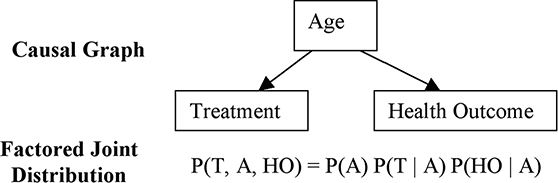
where the parents of $X_{i}$ are the immediate causes of $X_{i}$ , and if there are no parents then the marginal distribution $\mathrm{P}\,(X_{i}) $ is used. For example, consider Figure 1.

Figure 1.—

A causal graph.

The faithfulness assumption says that the causal graph represents the causal independence relations true in the population, that is, that there are no two causal paths that cancel each other out. However, several other conditions have to be specified in order to formulate a causal discovery problem precisely.

It is often assumed that the causal models under consideration satisfy causal sufficiency and acyclicity. Causal sufficiency is the assumption that there are no unmeasured common causes of any pair of variables that are under consideration (no latent confounders). Assuming causal sufficiency is unrealistic in most cases, since we rarely measure all common causes of all of our pairs of variables. However, the assumption has a large effect on a discovery procedure, since it reduces the space of models under consideration substantially. Assuming acyclicity prohibits models with feedback. While this may also be an unrealistic assumption—in many situations in nature there are feedback cycles—this is beyond the scope of this paper.

With these assumptions in place we turn to ‘structural’ and ‘parametric’ interventions. The typical intervention in medical trials is a ‘structural’ randomization of one variable. Subjects are assigned to the treatment or control group based on a random procedure, for example, a flip of a coin. We call the intervention “structural” because it alone completely determines the probability distribution of the target variable. It makes the intervened variable independent of its other causes and therefore changes the causal structure of a system before and after such an intervention. In a drug trial, for example, a fair coin determines whether each subject will be assigned one drug or another or a placebo. The assignment of treatment is independent of any other factor that might cause the outcome.Footnote ¹ Randomization of this kind ensures that, at least in the probability distribution true of the population, such a situation does not arise.

In Causal Bayes Nets a structural intervention is represented as an exogenous variable I (a variable without causes) with two states (on/off) and a single arrow into the variable it manipulates.Footnote ² When I is off, the passive observational distribution obtains over the variables. When I is on, all other arrows incident on the intervened variable are removed, and the probability distribution over the intervened variable is a determinate function of the intervention only. This property underlies the terminology “structural.”Footnote ³ If there are multiple simultaneous structural interventions on variables in the graph, the manipulated distribution for each intervened variable is independent of every other manipulated distribution,Footnote ⁴ and the edge breaking process is applied separately to each variable. This implies that all edges between variables that are subject to an intervention are removed. After removing all edges from the original graph incident to variables that are the target of a structural intervention, the resulting graph is called the postmanipulation graph and represents what is called the manipulated distribution over the variables.

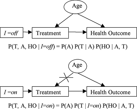
More formally, we have the following definition for a structural intervention $I_{s}$ on a variable X in a system of variables V (see Figure 2):

• • $I_{s}$ is a variable with two states (on/off).

• • When $I_{s}$ is off, the passive observational distribution over V obtains.

• • $I_{s}$ is a direct cause of X and only X.

• • $I_{s}$ is exogenous,Footnote ⁵ that is, uncaused.

• • When $I_{s}$ is on, $I_{s}$ makes X independent of its causes in V (breaks the edges that are incident on X) and determines the distribution of X; that is, in the factored joint distribution $\mathrm{P}\,(\boldsymbol{V}) $ , the term $\mathrm{P}\,(X\vert \mathrm{parents}\,(X)) $ is replaced with the term $\mathrm{P}\,(X\vert I_{s}) $ , all other terms in the factorized joint distribution are unchanged.

Figure 2.—

Causal Bayes Net representing a ‘structural’ intervention (e.g., a medical trial) where Treatment (T) and Health Outcome (HO) are confounded by an unmeasured common cause Age (A). When the intervention variable I is set to off, the passive observational distribution obtains over the variables. When it is set to on, the structural intervention breaks any arrows incident on the treatment variable, thereby destroying any correlation due to unmeasured common causes.

The epistemological advantages of structural interventions on one variable are at least the following:

• • No correlation between the manipulated variable and any other non-manipulated variable in the resulting distribution is due to an unmeasured common cause (confounder).

• • The structural intervention provides an ordering that allows us to distinguish the direction of causation, that is, it distinguishes between A → B and A ← B.

• • The structural intervention provides a fixed known distribution over the treatment variable that can be used for further statistical analysis, such as the estimation of a strength parameter of the causal link.

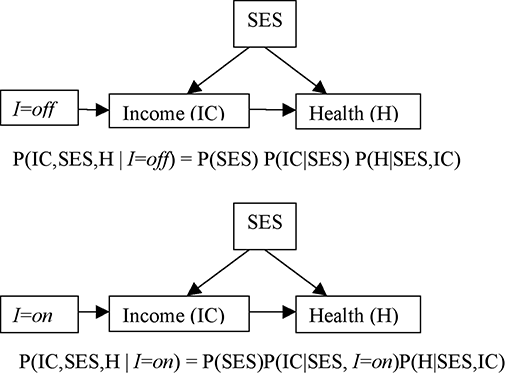
This is not the only type of intervention that is possible or informative, however. There may also be ‘soft’ interventions that do not remove edges, but simply modify the conditional probability distributions of the intervened upon variable. In a causal Bayes net, such an intervention would still be represented by an exogenous variable with a single arrow into the variable it intervenes on. Again, when it is set to off, the passive observational distribution obtains; but when it is set to on, the distribution of the variable conditional on its causes (graphical parents) is changed, but their causal influence (the incoming arrows) are not broken. We refer to such an intervention as a ‘parametric’ intervention, since it only influences the parameterization of the conditional probability distribution of the intervened variables on its parents, while it still leaves the causal structure intact.Footnote ⁶ The conditional distribution of the variable still remains a function of the variable's causes (parents).

More formally, we have the following definition for a parametric intervention $I_{p}$ on a variable X in a system of variables V (see Figure 3):

• • $I_{p}$ is a variable with two states (on/off).

• • When $I_{p}$ is off, the passive observational distribution over V obtains.

• • $I_{p}$ is a direct cause of X and only X.

• • $I_{p}$ is exogenous, that is, uncaused.

• • When $I_{p}$ is on, $I_{p}$ does not make X independent of its causes in V (does not break the edges that are incident on X). In the factored joint distribution $\mathrm{P}\,(\boldsymbol{V}) $ , the term $\mathrm{P}\,(X\vert \mathrm{parents}\,(X)) $ is replaced with the term $\mathrm{P}\,(X\vert \mathrm{parents}\,(X),\quad I_{p}=on) $ ,Footnote ⁷ and otherwise all terms are unchanged.

Figure 3.—

Causal Bayes Net representing a ‘parametric’ intervention. When the intervention variable I is set to off, the passive observational distribution obtains over the variables. When it is set to on, the parametric intervention does not break any arrows incident on the intervened variable, but only changes the conditional distribution of that variable. So, P(IC|SES) ≠ P(IC|SES, $I=on$ ). In contrast to structural interventions, parametric interventions do not break correlations due to unmeasured common causes.

There are several ways to instantiate such a parametric intervention. If the intervened variable is a linear (or additive) function of its parents, then the intervention could be an additional linear factor. For example, if the target is income, the intervention could be to boost the subject's existing income by $10,000/year. In the case of binary variables, the situation is a little more complicated, since the parameterization over the other parents must be changed, but even here it is possible to perform a parametric intervention, for example, by inverting the conditional probabilities of the intervened variable when the parametric intervention is switched to on.Footnote ⁸

3. Results.

While a structural intervention is extremely useful to test for a direct causal link between two variables (this is the focus in the statistics literature), it is not straight forwardly the case that structural interventions on single variables provide an efficient strategy for discovering the causal structure among several variables. The advantage it provides, namely making the intervened upon variable independent of its other causes, is also its drawback. In general, we still want a theory of causal discovery that does not rely upon an a priori separation of the variables into treatment and effect as is assumed in statistics. Even time ordering does not always imply information about such a separation, since we might only have delayed measures of the causes.

Faced with a setting in which any variable may be a cause of any other variable, a structural intervention of the wrong variable might then not be informative about the true causal structure, since even the manipulated distribution could have been generated by several different causal structures.

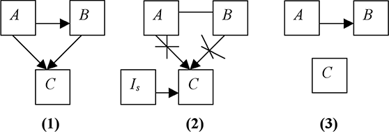
For example, consider Figure 4. Suppose the true but unknown causal graph is (1). A structural intervention on C would make the pairs A-C and B-C independent, since the incoming arrows on C are broken in the postmanipulation graph (2). The problem is that the information about the causal influence of A and B on C is lost. Note also, that an association between A and B is detected but the direction of the causal influence cannot be determined (hence the representation by an undirected edge). The manipulated distribution could as well have been generated by graph (3), where the true causal graph has no causal links between A and C or B and C. Hence, structural interventions also create Markov equivalence classes of graphs, that is, graphs that have a different causal structure, but imply the same conditional independence relations. (1) and (3) form part of an interventional Markov equivalence class under a structural intervention on C (they are not the only two graphs in that class, since the arrow between A and B could be reversed as well). Discovering the true causal structure using structural interventions on a single variable, and to be guaranteed to do so, requires a sequence of experiments to partition the space of graphs into Markov equivalence classes of unique graphs. Note that a further structural intervention on A in a second experiment would distinguish (1) from (3), since A and C would be correlated in (1) while they would be independent in (3).

Figure 4.—

Actual and manipulated causal graphs.

Eberhardt, Glymour, and Scheines (Reference Eberhardt, Glymour, Scheines, Holmes and Jain2006) showed that for N causally sufficient variables $N-1$ experiments are sufficient and in the worst case necessary to discover the causal structure among a causally sufficient set of N variables if at most one variable can be subjected to a structural intervention per experiment assuming faithfulness. If multiple variables can be randomized simultaneously and independently in one experiment, this bound can be reduced to $\mathrm{\log}_{2}(N) +1$ experiments (Eberhardt et al. Reference Eberhardt, Glymour, Scheines, Bacchus and Jaakkola2005). These bounds both assume that an experiment specifies a subset of the variables under consideration that are subject to an intervention and that each experiment returns the independence relations true in the manipulated population, that is, issues of sample variability are not addressed.

Parametric interventions do not destroy any of the causal structure. However, if only a single parametric intervention is allowed, then there is no difference in the number of experiments between structural and parametric interventions:

For experiments that can include simultaneous interventions on several variables, however, we can decrease the number of experiments from $\mathrm{\log}_{2}(N) +1$ to a single experiment when using parametric interventions:

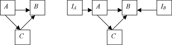
The following example, illustrated in Figure 5, explains the result: The true unknown complete graph among the variables A, B, and C is shown on the left. In one experiment, the researcher performs simultaneously and independently a parametric intervention on A and B ( $I_{A}$ and $I_{B}$ , respectively, shown on the right). Since the interventions do not break any edges, the graph on the right represents the postmanipulation graph. Note that A, B, and $I_{B}$ form an unshielded collider,Footnote ⁹ as do C, B, and $I_{B}$ . These can be identified (see footnote 9) and hence determine the edges and their directions A to B and C to B. The edge A to C can be determined since (i) A and C are dependent for all possible conditioning sets, but (ii) $I_{A}$ , A and C do not form an unshielded collider. Hence we can conclude that (from [i]) there must be an edge between A and C and (from [ii]) that it must be directed away from A. We have thereby managed to discover the true causal graph in one experiment. Essentially, adjacencies can be determined from observational data alone. The parametric interventions set up a ‘collider test’ for each triple I _X, X, and Y with X—Y adjacent, which orients the X—Y adjacency.

Figure 5.—

A true unknown causal graph and a postmanipulation graph.

4. Discussion.

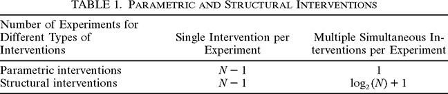
These results indicate that the advantage of parametric interventions lies with the fact that they do not destroy any causal connections. (See Table 1.)

Table 1.Parametric and Structural Interventions

Number of Experiments for Different Types of Interventions	Single Intervention per Experiment	Multiple Simultaneous Interventions per Experiment
Parametric interventions	$N-1$	1
Structural interventions	$N-1$	$\mathrm{\log}_{2}(N) +1$

The theorems tempt the conclusion that parametric interventions are always better than structural interventions. But this would be a mistake since the theorems hide the cost of this procedure. First, determining the causal structure from parametric interventions requires more conditional independence tests with larger conditioning sets. This implies that more samples are needed to obtain a similar statistical power on the independence tests as in the structural intervention case. Second, the above theorems only hold in general for causally sufficient sets of variables. A key advantage of randomized trials (structural interventions) is their robustness against latent confounders (common causes). Parametric interventions are not robust in this way, since they do not make the intervened variable independent of its other causes. This implies that there are cases for which the causal structure cannot be uniquely identified by parametric interventions.

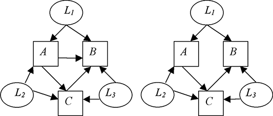
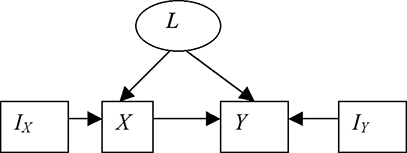
The two graphs in Figure 6 over the observed variables A, B and C with latent common causes $L_{1}$ , $L_{2}$ , and $L_{3}$ are indistinguishable given parametric interventions on A, B, and C. There is no conditional independence relation between the variables (including the intervention nodes omitted for clarity in the figure) that distinguishes the two graphs.Footnote ¹⁰ However, it is not always the case that causal insufficiency renders parametric interventions useless as the example in Figure 7 shows.

Figure 6.—

Two graphs with latent variables that are indistinguishable by parametric interventions on A, B, and C (the intervention variables are omitted for clarity).

Figure 7.—

Even in the presence of a latent variable, this causal structure can be uniquely determined with parametric interventions on X and Y in a single experiment.

The parametric intervention $I_{X}$ on X will not break the association between X and Y that is due to the unmeasured common cause L. This does not mean that the edge X to Y cannot be identified, since (a) if there were no edge between X and Y, then $I_{X}$ and Y would not be associated, and (b) if the edge were from Y to X, then $I_{Y}$ and X would be associated.Footnote ¹¹ As the two examples show, parametric interventions are sometimes subject to failure when causal sufficiency cannot be assumed, but this depends very much on the complexity of the model.Footnote ¹² It follows that the assumption of causal sufficiency does not compensate entirely for what parametric interventions lack in robustness to unmeasured common causes. First, the results for structural interventions also depend on causal sufficiency. (See Eberhardt et al. Reference Eberhardt, Glymour, Scheines, Bacchus and Jaakkola2005.) A logarithmic bound on the number of experiments when using structural interventions would not be achievable in the worst case if there are latent common causes. Second, there are cases (as the example above shows) where parametric interventions are still sufficient to recover the causal structure even if there are latent common causes.Footnote ¹³ In some cases one can even identify the location of the latent variables. However, this is not always the case and we do not have any general theorem of these cases to report at this stage. What seems to play a much larger role than causal sufficiency is the requirement of exogeneity of the intervention. It results in additional independence constraints (creating unshielded colliders) whose presence or absence make associations identifiable with direct causal connections.

The moral is that while the types of interventions are not independent of the assumptions that are made about causal sufficiency, they are not interchangeable with them either. It is not the case that causal sufficiency and parametric interventions achieve the same search capability as causal insufficiency and structural interventions. The tradeoffs are rather subtle and we have only shown a few examples of the interplay of some of the assumptions. But there does not seem to be any general sense in which one can speak of ‘weaker’ or ‘stronger’ interventions with regard to their epistemological power.