1 Introduction
The stability of a cantilevered thin elastic sheet immersed in a steady uniform flow has received widespread attention due to its relevance in many applications, ranging from the aerodynamics of flight to understanding the basic dynamics of flag motion (Theodorsen Reference Theodorsen1935; Kornecki, Dowell & O’Brien Reference Kornecki, Dowell and O’Brien1976; Guo & Paidoussis Reference Guo and Paidoussis2000; Zhang et al. Reference Zhang, Childress, Libchaber and Shelley2000; Eloy et al. Reference Eloy, Lagrange, Souilliez and Schouveiler2008; Manela & Howe Reference Manela and Howe2009; Paidoussis, Price & De Langre Reference Paidoussis, Price and De Langre2010). The predominant configuration studied to date is that where the flow (i) impinges on the sheet’s clamped end, and (ii) is parallel to the sheet; mimicking the orientation often encountered by flags and biological structures that naturally position themselves in the flow direction. This configuration will henceforth be referred to as the ‘conventional flag’ problem; as opposed to the ‘inverted flag’ reported by Kim et al. (Reference Kim, Cosse, Huertas Cerdeira and Gharib2013) which is the focus of this study. Shelley & Zhang (Reference Shelley and Zhang2011) review the extensive body of literature on the conventional flag problem, which encompasses theoretical and experimental work; both clamped and pinned flags have been considered. While this problem has been studied widely over the past century, the effects of orientation on the resulting sheet dynamics have received comparatively little attention.
Recent measurements by Kim et al. (Reference Kim, Cosse, Huertas Cerdeira and Gharib2013) show that reversing the orientation of a cantilevered thin elastic sheet, with its length parallel to a steady uniform flow at high Reynolds numbers (
 $\mathit{Re}\equiv UL/{\it\nu}\approx 10^{4}{-}10^{5}$
), can dramatically alter the sheet’s stability and resulting dynamics;
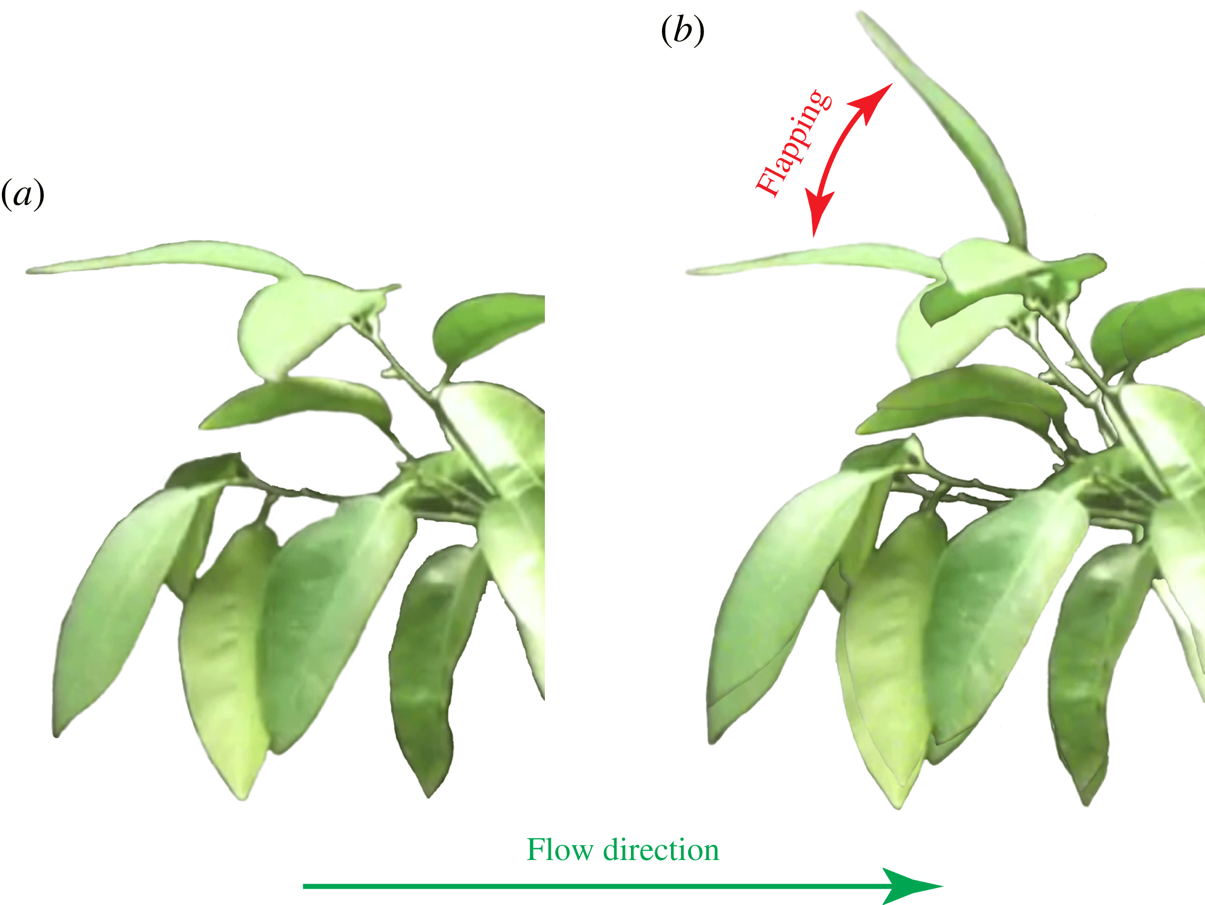
 $U$
is the flow speed,
 $L$
the sheet length and
 ${\it\nu}$
the fluid’s kinematic viscosity. The physical mechanisms underlying the observed behaviour of this inverted flag remain unknown. The aim of this article is to shed light on these mechanisms and thus provide insight into the effects of flow orientation on a cantilevered elastic sheet’s dynamics.
These effects of flow orientation were recently examined for a cantilevered slender circular cylinder oriented in a reverse configuration parallel to the flow (Rinaldi & Paidoussis Reference Rinaldi and Paidoussis2012) – as for the inverted flag. The dynamics of this ‘inverted rod’ differ greatly from that of a conventional flag, with small-amplitude flutter oscillations (amplitude less than the cylinder diameter) occurring at low flow speeds. This small-amplitude motion gives way to an abrupt deflected equilibrium at higher speeds. The authors of that study suggest that this bifurcation is due to a static divergence. The predicted critical flow speed based on a theoretical model significantly exceeds their experimental observations.
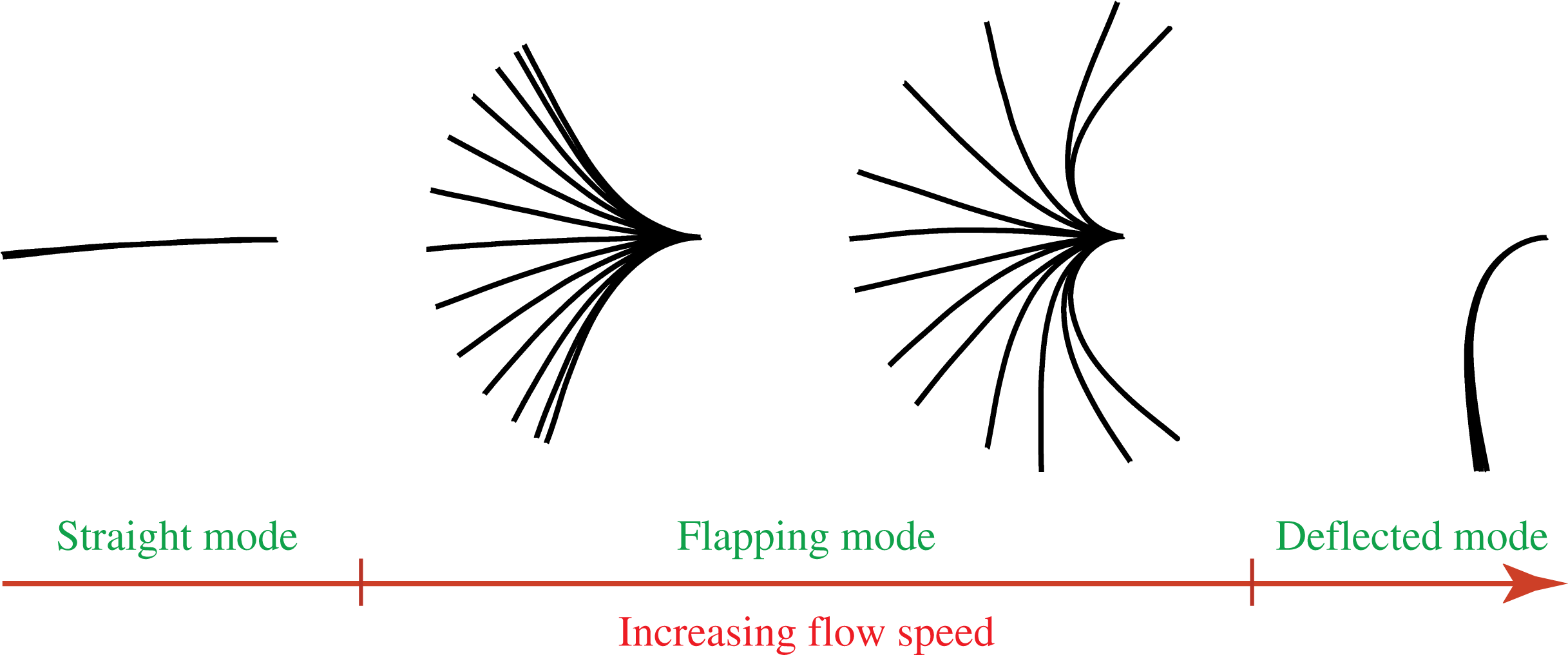
This inverted-rod behaviour contrasts strongly with that observed by Kim et al. (Reference Kim, Cosse, Huertas Cerdeira and Gharib2013) for the inverted flag. The inverted flag also exhibits an undeflected and stable zero-deflection equilibrium at low flow speeds. However, as the flow speed increases, this equilibrium gives way abruptly to large-amplitude flapping motion of the sheet; this amplitude is comparable to the sheet’s length, and thus many orders of magnitude larger than its thickness (the oscillation amplitude of an inverted rod). As the flow speed is increased further, this flapping motion ceases (also abruptly), resulting in a stable deflected equilibrium of the sheet. Figure 1 shows this evolution as a function of flow speed; measurements are taken from Kim et al. (Reference Kim, Cosse, Huertas Cerdeira and Gharib2013). This comparison of the inverted-flag and inverted-rod dynamics shows that cantilever geometry plays a major role in dictating overall stability and dynamics. Onoue et al. (Reference Onoue, Song, Strom and Breuer2015) recently observed that a rigid plate mounted in a torsion spring similarly exhibits large-amplitude angular oscillations over a finite flow speed range. Buchak, Eloy & Reis (Reference Buchak, Eloy and Reis2010) studied the stability and dynamics of a ‘clapping book’, which has narrow thin sheets also in a reverse flow orientation (as for the inverted flag and inverted rod), but gravity rather than elasticity play a dominant role in that case. Here, we are interested in the situation where gravity has a negligible effect; see below.
Stroboscopic measurements of an inverted flag as a function of increasing flow speed; edge view of the elastic sheet, which is clamped on its right-hand side, with the flow impinging on its left-hand free edge. These measurements, taken in air, show the abrupt transition of a stable zero-deflection equilibrium (straight mode – left-most image) at low flow speed, to a flapping mode (middle two images) and ultimately to a stable deflected mode (right-most image), with increasing flow speed. Images taken from figure 2(c) of Kim et al. (Reference Kim, Cosse, Huertas Cerdeira and Gharib2013), where measurement specifications are provided.

Considerable effort has been spent on theoretically modelling and experimentally measuring the statics and dynamics of thin elastic sheets in flow. On the theoretical front, simplified fluid-structure models exist that use an inviscid formulation for the hydrodynamics, due to the high Reynolds numbers involved, as well as fully numerical studies that directly tackle the coupled Navier–Stokes (fluid) and Navier (solid) equations; see Shelley & Zhang (Reference Shelley and Zhang2011) for a review. The first analytical approach was by Theodorsen (Reference Theodorsen1935), who used unsteady thin airfoil theory to investigate the stability of elastically mounted rigid panels. Kornecki et al. (Reference Kornecki, Dowell and O’Brien1976) provided an elegant treatment of the two-dimensional elastic sheet problem, yielding insight into the stability of the conventional flag; this important work appears to have gone unnoticed in more recent times, with some of their results being reproduced (inaccurately), as we shall discuss. Jones (Reference Jones2003) tackled the problem of flow separation in an inviscid fluid due to a moving flat plate, which has been used in a number of contexts (Jones & Shelley Reference Jones and Shelley2005; Michelin, Llewellyn Smith & Glover Reference Michelin, Llewellyn Smith and Glover2008; Buchak, Eloy & Reis Reference Buchak, Eloy and Reis2009). In this article, we draw on parts of this literature and extend it to explain the main physical mechanisms underlying the dynamics of the inverted flag phenomenon reported by Kim et al. (Reference Kim, Cosse, Huertas Cerdeira and Gharib2013). We are not so much interested in modelling the complete flow, which in principle can be done using the fully numerical or semi-analytical approaches developed previously, but using the most fundamental theoretical and experimental tools to extract the essential physics of the inverted flag phenomenon. Indeed, a very recent computational study by Gilmanov, Le & Sotiropoulos (Reference Gilmanov, Le and Sotiropoulos2015) used an LES formulation to simulate inverted flag flapping at the high Reynolds numbers measured by Kim et al. (Reference Kim, Cosse, Huertas Cerdeira and Gharib2013), i.e.
 $\mathit{Re}\approx 10^{4}{-}10^{5}$
. Others have performed direct numerical simulations of the Navier–Stokes equations and thus focus on low Reynolds number flows (
 $\mathit{Re}\approx 100{-}200$
) (Ryu et al.
Reference Ryu, Park, Kim and Sung2015; Tang, Liu & Lu Reference Tang, Liu and Lu2015). While these computational studies were able to reproduce the phenomena observed experimentally, the dominant physical mechanisms were notdescribed.
Interestingly, the measurements we present show that flapping of an inverted flag can exhibit a transition to chaos with increasing flow speed, analogous to previous observations for conventional flags (Connell & Yue Reference Connell and Yue2007; Alben & Shelley Reference Alben and Shelley2008; Michelin et al. Reference Michelin, Llewellyn Smith and Glover2008; Ait Abderrahmane et al. Reference Ait Abderrahmane, Paidoussis, Fayed and Ng2012; Chen et al. Reference Chen, Jia, Wu, Yin and Ma2014). This study therefore highlights some of the similarities and differences between the dynamics of conventional and inverted flags.
Flow past a bluff body at high Reynolds number is well known to exhibit periodic vortex shedding for the Reynolds numbers under consideration here, i.e.
 $\mathit{Re}\approx 10^{4}{-}10^{5}$
(Fage & Johansen Reference Fage and Johansen1927; Schmitz Reference Schmitz1941; Roshko Reference Roshko1954; Knisely Reference Knisely1990). This is not only true for circular cylinders, but for other shapes of comparable ‘bluffness’ (Roshko Reference Roshko1954). As such, the inverted flag also exhibits periodic vortex shedding when deflected from its zero-deflection equilibrium, because it too presents a bluff body to the flow; geometrically it is a thin sheet with high curvature and sharp edges, ensuring flow separation and vortex shedding. This vortex shedding will periodically force the elastic sheet. It is therefore entirely possible that this forcing can synchronise with the sheet motion, leading to a vortex-induced vibration (Williamson & Govardhan Reference Williamson and Govardhan2004; Gabbai & Benaroya Reference Gabbai and Benaroya2005), albeit with a geometry that varies strongly as the sheet oscillates – in contrast to that of a constant cross-section elastic rod at perpendicular incidence to the flow, that has been studied widely. Kim et al. (Reference Kim, Cosse, Huertas Cerdeira and Gharib2013) noted that the inverted flag’s trend in oscillation (flapping) over a finite range of flow speeds is somewhat analogous to the vortex-induced vibration (VIV) of a cylinder (Shiels, Leonard & Roshko Reference Shiels, Leonard and Roshko2001), though this connection was not explored.
Here, we investigate this similarity in detail by drawing on the existing VIV literature, combining it with detailed measurements and scaling arguments, and thus test the hypothesis that flapping of an inverted flag is indeed a VIV. This motion could in principle be modelled theoretically using existing frameworks (above), but is complicated by the analytical intractability of the resulting coupled elastic/fluid equations for such a separated flow; also approximations inherent in any such formulation can convolute the resulting conclusions. We therefore prefer a detailed experimental exploration of the flapping region, involving a host of new measurements coupled with a scaling analysis, to investigate the hypothesis that flapping is a VIV. As we shall show, motion in the flapping region exhibits the required properties of a VIV, providing strong evidence for its existence.
This article is arranged as follows. We begin in § 2 with an exposition of the experimental set-up used to generate the new measurements. This data is used to explore the mechanisms underlying the dynamics observed by Kim et al. (Reference Kim, Cosse, Huertas Cerdeira and Gharib2013). Initially, we extend the measurements of Kim et al. (Reference Kim, Cosse, Huertas Cerdeira and Gharib2013) to examine the effects of sheet aspect ratio (height/length) – this sets the stage for the remainder of the study. The flow speed at which flapping is initiated (at low speed; see figure 1) is examined theoretically in § 3. The model of Kornecki et al. (Reference Kornecki, Dowell and O’Brien1976) is contrasted against a more recent theoretical treatment by Argentina & Mahadevan (Reference Argentina and Mahadevan2005) – the latter is shown to be a subset of the former but involves inaccurate approximation; the framework of Kornecki et al. (Reference Kornecki, Dowell and O’Brien1976) is therefore used throughout. The theoretical model for the inverted flag is first developed for a two-dimensional sheet, and then extended to account for finite sheet aspect ratio using Prandtl’s lifting-line theory and the vortex lattice method (Anderson Reference Anderson1991). A detailed comparison of this model to the new measurements, as a function of aspect ratio, is presented. In § 4, we turn our attention to the flapping region, where new detailed measurements of the motion and a scaling analysis are reported. This combined approach leads us to conclude that flapping is a VIV. The aperiodic and chaotic motion of the inverted flag is then explored, and compared to the dynamics of a conventional flag. Finally, in § 5 we comment on the connection of the inverted flag’s dynamics to biological phenomena such as the motion of tree leaves. We conclude in § 6 with a summary of the findings of this study.
2 Experimental details
2.1 Apparatus
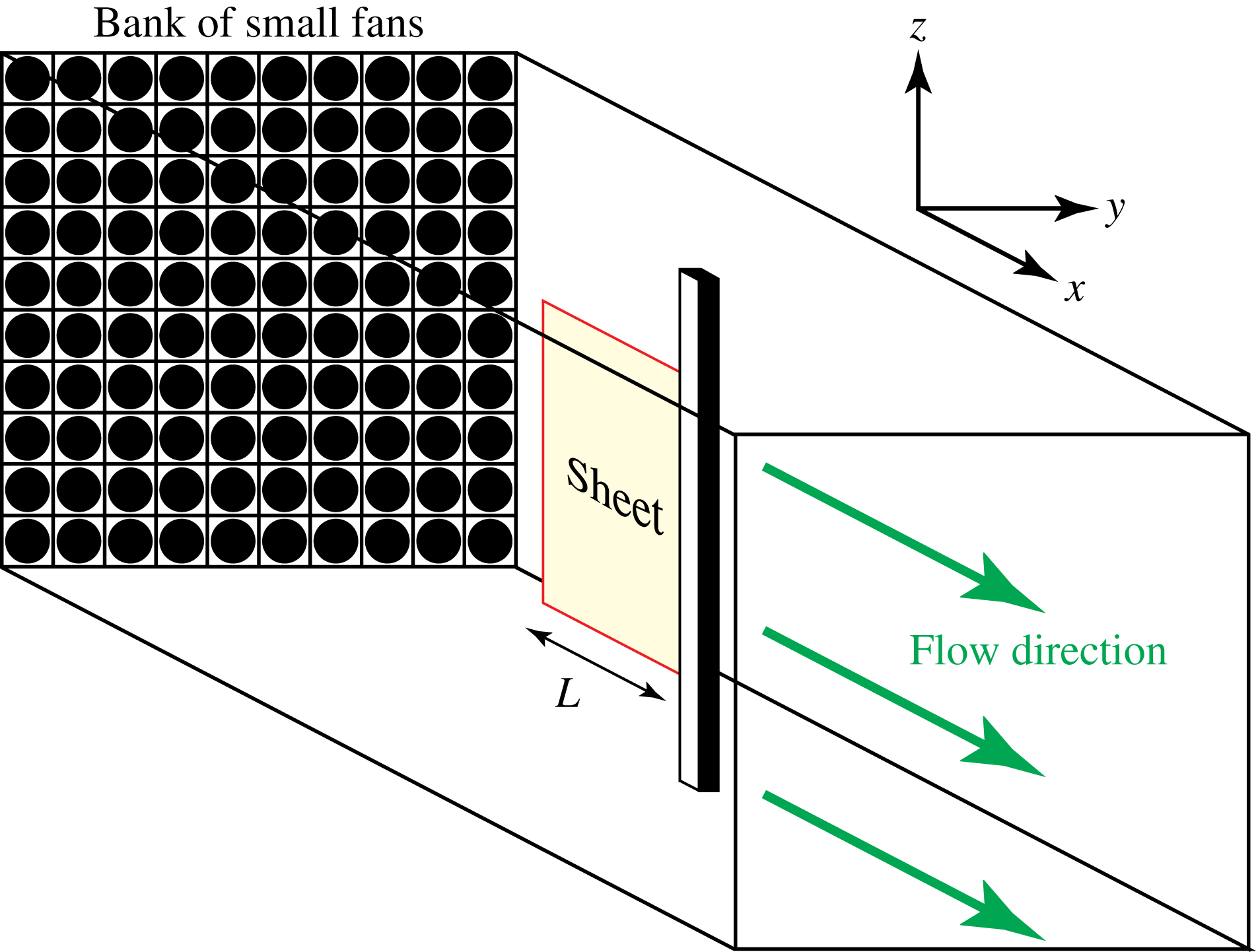
A schematic of the measurement set-up used to study the motion of the inverted flag in a steady uniform flow is provided in figure 2; this is identical to that used by Kim et al. (Reference Kim, Cosse, Huertas Cerdeira and Gharib2013). A large array (
 $10\times 10$
) of small computer fans, aligned side-by-side, form a vertical bank that provides the steady flow that impinges on the free edge of the inverted flag (a thin elastic sheet). The opposite edge of the sheet is clamped into a rigid aluminium cylindrical support of square cross-section. An aluminium honeycomb is used as a flow straightener to reduce transverse and axial fluctuation generated by the fans. The streamwise width of the honeycomb is 3.8 cm and the diameter of each cell in the honeycomb is 0.6 cm. Hot-wire measurements show that turbulence levels are below 9 %. The new measurements are performed in air, extending those reported previously by Kim et al. (Reference Kim, Cosse, Huertas Cerdeira and Gharib2013). For operation in water, we draw on the existing data of Kim et al. (Reference Kim, Cosse, Huertas Cerdeira and Gharib2013).
Kim et al. (Reference Kim, Cosse, Huertas Cerdeira and Gharib2013) reported measurements of thin sheets of fixed thickness with aspect ratios (height/length) close to unity (1–1.3). Consequently, those previous measurements do not shed light on the effect of sheet geometry. Here, we extend these measurements using sheets whose thickness (and length) differ by a factor of six, and vary their aspect ratio over two orders of magnitude. In all cases, the sheet’s thickness is much smaller than its length and height.
Schematic illustration of the measurement apparatus used to investigate the stability and dynamics of an inverted flag in a uniform steady air flow. A high speed camera is placed on top of the apparatus, thus viewing the sheet edge on. This enables stroboscopic images of the sheet’s motion to be captured. Cartesian coordinate system used in theoretical analysis and measurement interpretation is shown; the origin is at the free end of the sheet (for the inverted flag only – the origin is at the clamped end for a conventional flag). The length of the sheet is
 $L$
(indicated), whereas its height in the vertical direction is
 $H$
(not shown).

The sheets used as inverted flags are fashioned from larger sheets of polycarbonate, with Young’s modulus
 $E=2.4$
GPa, Poisson’s ratio
 ${\it\nu}=0.38$
and density
 ${\it\rho}_{s}=1200~\text{kg}~\text{m}^{-3}$
. Air density is
 ${\it\rho}=1.2~\text{kg}~\text{m}^{-3}$
. The resulting elastic sheets are chosen to have two lengths,
 $L=5.1$
and 30 cm, with sheet thicknesses
 $h=0.13$
mm and 0.78 mm, respectively, giving identical values for
 $h/L$
; this property is employed in the measurement analysis that follows. The sheet flexural rigidity used in this study is defined
 $D\equiv Eh^{3}/(12[1-{\it\nu}^{2}])$
. The heights of the sheets are varied in the range
 $H=2.5{-}62$
cm, yielding aspect ratios
 $0.1\leqslant H/L\leqslant 7.5$
. The larger thickness sheet is nominally identical to that of Kim et al. (Reference Kim, Cosse, Huertas Cerdeira and Gharib2013), though not the same sheet. The sixfold variation in sheet size alters the Reynolds number by the same factor, allowing the effect of Reynolds number to be investigated at identical air flow speeds. The flow speed is varied from
 $U=2.5$
to
 $8.5~\text{m}~\text{s}^{-1}$
. The sheet’s motion is measured using a high-speed camera (100 f.p.s.) placed at the top of the test section. The length of the sheet,
 $L$
, is aligned in the flow direction (
 $x$
-direction), its height,
 $H$
, is in the direction of gravity (negative
 $z$
-direction) and its thickness,
 $h$
, is in the
 $y$
-direction; see figure 2. Gravity does not distort any of the sheets from their free standing vertical shapes. For convenience, we shall often use the term ‘sheet’ to refer to a conventional or inverted flag; the meaning being implicit from the context of the discussion.
2.2 Measurements as a function of the sheet’s aspect ratio,
 $H/L$

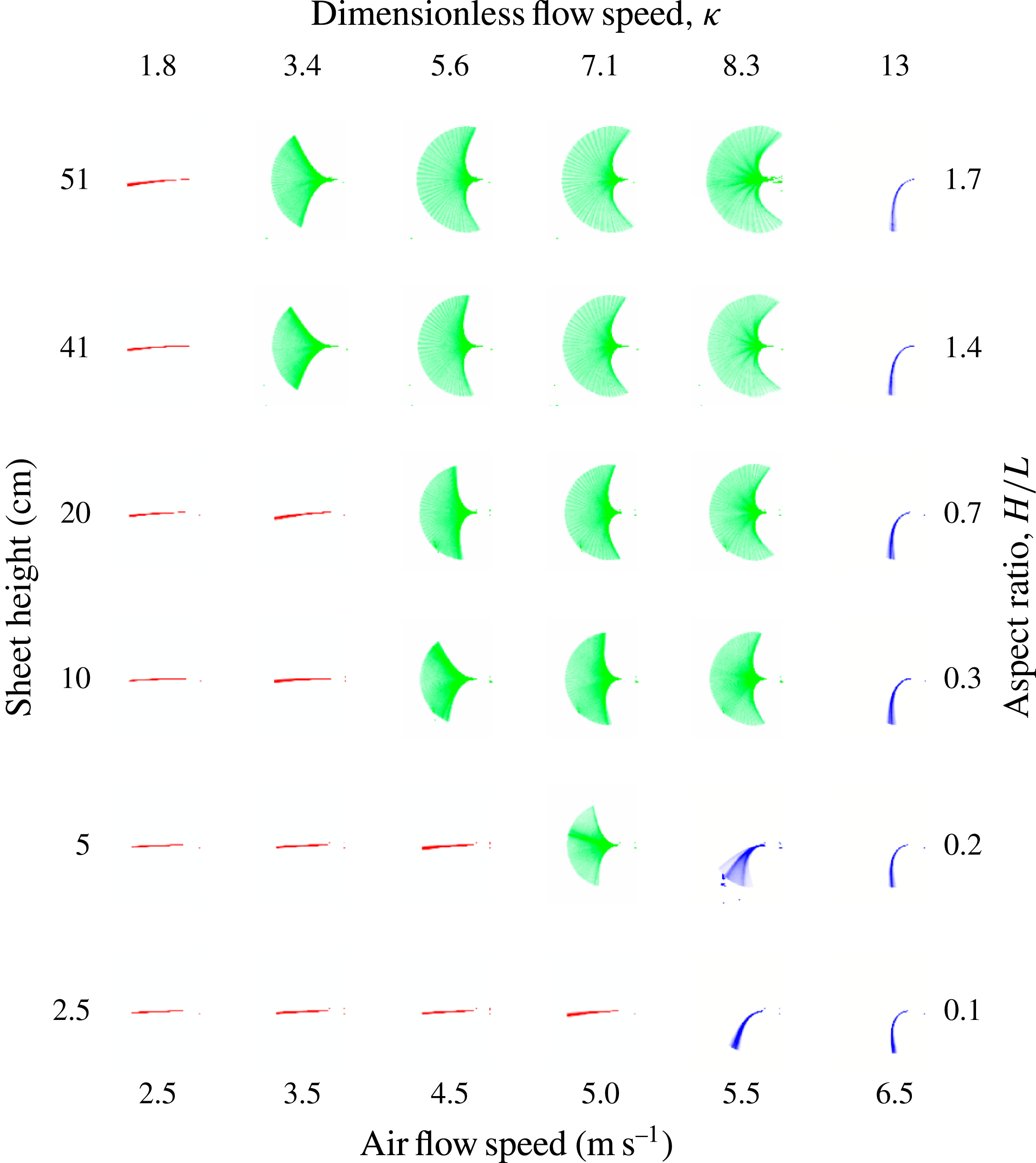
Figure 3 presents stroboscopic measurements of the inverted flag’s motion, taken using the above described apparatus, as a function of sheet height (and thus aspect ratio) and air flow speed; the dimensionless flow speed
 ${\it\kappa}$
is defined in (3.1). Results for the larger inverted flags of thickness
 $h=0.78$
mm are shown, and thus provide a direct extension of the measurements reported previously (Kim et al.
Reference Kim, Cosse, Huertas Cerdeira and Gharib2013). As described by Kim et al. (Reference Kim, Cosse, Huertas Cerdeira and Gharib2013), increasing the flow speed causes the sheet to move from a stable undeformed equilibrium to large-amplitude flapping; as in figure 1. This occurs abruptly at a critical flow speed,
 $U_{\mathit{lower}}$
. When the flow speed is increased further, a second abrupt transition occurs at
 $U_{\mathit{upper}}$
where large-amplitude flapping ceases and a steady deflection is recovered, at large amplitude; a small amount of flutter is also observed in this deflected equilibrium. This deflected equilibrium is observed to occur on one side only, and is due to small and unavoidable curvature in the sheet; pushing the sheet to the other side yields a similar deflection.
These measurements, at constant sheet length, show that the sheet dynamics are strongly affected by the sheet’s height, and thus its aspect ratio, with
 $U_{\mathit{lower}}$
increasing with decreasing aspect ratio. In contrast,
 $U_{\mathit{upper}}$
appears to be insensitive to the sheet’s aspect ratio. This establishes that the sheet geometry can dramatically affect its dynamics, with flapping appearing only if the sheet’s aspect ratio exceeds a critical value. For smaller aspect ratios, a direct transition to a stable deflected equilibrium occurs. Our theoretical analysis focuses on sheets of high aspect ratio, with a brief discussion of the low aspect ratio case.
These results differ from those of a conventional flag, which is always unstable above a critical flow speed (Theodorsen Reference Theodorsen1935; Kornecki et al. Reference Kornecki, Dowell and O’Brien1976; Guo & Paidoussis Reference Guo and Paidoussis2000; Zhang et al. Reference Zhang, Childress, Libchaber and Shelley2000; Paidoussis et al. Reference Paidoussis, Price and De Langre2010; Shelley & Zhang Reference Shelley and Zhang2011). But the measurements in figure 3 are consistent with the findings of Rinaldi & Paidoussis (Reference Rinaldi and Paidoussis2012), who considered the inverted-rod problem, i.e. a slender (cylindrical cross-section) elastic rod of small aspect ratio, which also did not display flapping behaviour; see § 1.
We now examine the physical mechanisms underlying the behaviour observed in figure 3.
Stroboscopic images of the sheet motion as a function of sheet height and air flow speed, for the
 $L=30$
cm sheets. Dimensionless flow speed,
 ${\it\kappa}$
, and sheet aspect ratio,
 $H/L$
, are also indicated. Stable equilibrium states are observed at low (red) and high (blue) flow speeds, whereas large-amplitude flapping occurs at intermediate flow speeds (green). Flow direction is left to right, and the sheet is clamped at its right-hand end.

3 Stability at low flow speed
We begin by investigating the onset of flapping at low flow speed, i.e. at
 $U_{\mathit{lower}}$
. To theoretically explore the physical mechanisms driving
 $U_{\mathit{lower}}$
, we draw on the study of Kornecki et al. (Reference Kornecki, Dowell and O’Brien1976). As noted in § 1, Argentina & Mahadevan (Reference Argentina and Mahadevan2005) presented an analysis similar to that of Kornecki et al. (Reference Kornecki, Dowell and O’Brien1976), though this similarity has not been discussed in the literature.
3.1 Theories of Kornecki et al. (Reference Kornecki, Dowell and O’Brien1976) and Argentina & Mahadevan (Reference Argentina and Mahadevan2005)
Both Kornecki et al. (Reference Kornecki, Dowell and O’Brien1976) and Argentina & Mahadevan (Reference Argentina and Mahadevan2005) explored the stability of the conventional flag problem. The fundamental theoretical frameworks of these complementary studies are identical, which appears to have gone unnoticed. Specifically, these studies utilise the small-deflection theory for thin elastic plates, steady and unsteady thin airfoil theory, and assume the sheet is infinitely wide (resulting in a two-dimensional formulation).
However, Argentina & Mahadevan (Reference Argentina and Mahadevan2005) make the overriding assumption that the sheet’s displacement varies slowly along its length, in the direction of flow, i.e. the
 $x$
-direction. This enables approximation of the hydrodynamic pressure load by one that depends only on the local sheet displacement (at a particular value of
 $x$
), rather than a convolution integral over the complete displacement field, as expected for a 2-D potential flow. The approximation is equivalent to replacing each infinitesimal line section of the deflected sheet (which is curved in the
 $x$
-direction) by a straight sheet rotated about the
 $z$
-axis that is of identical length to the original sheet. Since the sheet’s displacement varies from zero at its clamp to a finite value at its free edge, the deflection cannot a priori be considered small and this approximation can therefore introduce significant error. Indeed, the equation-of-motion in equation (18) of Argentina & Mahadevan (Reference Argentina and Mahadevan2005) is recovered from that of Kornecki et al. (Reference Kornecki, Dowell and O’Brien1976) ((3.2) below) under this approximation.
We therefore utilise the work of Kornecki et al. (Reference Kornecki, Dowell and O’Brien1976) in this study.
3.2 Two-dimensional sheet (infinite aspect ratio)
To explore the sheet’s stability at low flow speed, we initially study the limiting case of infinite aspect ratio,
 $H/L$
. This two-dimensional problem is relevant to understanding the practical case where the sheet’s height greatly exceeds its length; see figure 2.
Kornecki et al. (Reference Kornecki, Dowell and O’Brien1976) and others (see Shelley & Zhang (Reference Shelley and Zhang2011) for a review) have shown that the stability of a conventional flag depends on two parameters:
 $$\begin{eqnarray}{\it\kappa}\equiv \frac{{\it\rho}U^{2}L^{3}}{D},\quad {\it\mu}\equiv \frac{{\it\rho}L}{{\it\rho}_{s}h},\end{eqnarray}$$
where
 ${\it\kappa}$
specifies the ratio of hydrodynamic to elastic restoring forces (henceforth referred to as the ‘dimensionless flow speed’, for simplicity), and
 ${\it\mu}$
is the relative importance of fluid-to-solid inertia (termed the ‘added mass parameter’); all other variables are defined in § 2.1.
By calculating the pressure distribution along the sheet, using both steady and unsteady thin airfoil theory, Kornecki et al. (Reference Kornecki, Dowell and O’Brien1976) performed a linear stability analysis of the zero-deflection equilibrium state of the conventional-flag problem – where the flow impinges on the clamped edge of the sheet. To analyse the inverted flag, the boundary conditions are reversed, with the flow now impinging on the sheet’s free edge.
While Kornecki et al. (Reference Kornecki, Dowell and O’Brien1976) used both steady and unsteady thin airfoil theory to account for the hydrodynamic load, we utilise the steady theory only here, the rationale for which is detailed below. This allows us to determine when steady and unsteady hydrodynamic processes are involved, while not unduly complicating the analysis. Note that (unsteady) inertia in the solid sheet is included fully in both formulations.
The steady theory of Kornecki et al. (Reference Kornecki, Dowell and O’Brien1976) yields the following integro-differential equation:
 $$\begin{eqnarray}\frac{\text{d}^{4}w}{\text{d}x^{4}}-{\it\Omega}^{2}w+2{\it\kappa}\frac{f({\it\theta})-f(0)}{\sin {\it\theta}}=0,\end{eqnarray}$$
where
 $w$
is the sheet deflection,
 $x$
the normalised Cartesian coordinate in the free-stream direction (scaled by the sheet length
 $L$
) and the dimensionless frequency is defined
 $$\begin{eqnarray}{\it\Omega}\equiv {\it\omega}\sqrt{\frac{{\it\rho}_{s}hL^{4}}{D}},\end{eqnarray}$$
where
 ${\it\omega}$
is the angular frequency of the sheet’s motion, and
 $$\begin{eqnarray}f({\it\theta})=\frac{1}{{\rm\pi}}\int _{0}^{{\rm\pi}}w^{\prime }({\it\zeta})\frac{\sin ^{2}{\it\phi}}{\cos {\it\phi}-\cos {\it\theta}}\,\text{d}{\it\phi},\end{eqnarray}$$
 $$\begin{eqnarray}x={\textstyle \frac{1}{2}}(1+\cos {\it\theta}),\quad {\it\zeta}={\textstyle \frac{1}{2}}(1+\cos {\it\phi}),\end{eqnarray}$$
with
 $x\in [0,1]$
and
 ${\it\theta},{\it\phi}\in [0,{\rm\pi}]$
; all other parameters are defined in § 2.1. Equation (3.2) is derived using the small-deflection theory for thin elastic plates (in the 2-D limit) incorporating a hydrodynamic pressure load for potential flow over a curved plate. The first term in (3.2) is the elastic restoring force of the plate (i.e. sheet), the second is the inertial load of the sheet (only) and the third term is the hydrodynamic load. This load is calculated from steady thin airfoil theory incorporating the Kutta condition at the trailing edge of the sheet, i.e. at
 $x=1$
(
 ${\it\theta}=0$
); see Kornecki et al. (Reference Kornecki, Dowell and O’Brien1976). Note that the hydrodynamic load is approximated by its steady solution, whereas inertia in the solid sheet is retained. The associated boundary conditions are discussed below.
While flow separation is expected at the (sharp) leading free edge of the inverted flag, the above inviscid theory will hold provided the deflection is not too large. The reason is that a small deflection of the sheet will produce a small (attached) separation bubble at the sheet’s surface, and thus a predominantly inviscid flow (Schmitz Reference Schmitz1941). Indeed, measurements show that steady thin airfoil theory accurately captures the lift of a stationary thin flat sheet for the Reynolds numbers under consideration here (
 $\mathit{Re}\approx 10^{4}{-}10^{5}$
) and angles of attack
 ${\lesssim}10^{\circ }$
(Pelletier & Mueller Reference Pelletier and Mueller2000).
3.2.1 Rationale for use of Kornecki’s steady theory
The utility of using Kornecki’s steady theory, (3.2), is as follows:
-
(i)
${\it\Omega}\neq 0$
: if (3.2) predicts a bifurcation at non-zero frequency,
${\it\Omega}$
, then unsteadiness in the hydrodynamic pressure load may affect the sheet’s stability. Consequently, terms describing the unsteady hydrodynamic load, which involve the added mass parameter
${\it\mu}$
, must be included, i.e. the full unsteady theory of Kornecki et al. (Reference Kornecki, Dowell and O’Brien1976) must be used. -
(ii)
${\it\Omega}=0$
: bifurcation at zero frequency,
${\it\Omega}=0$
, establishes that the true hydrodynamic load is steady at bifurcation. That is, the steady approximation to the hydrodynamic load in (3.2) is exact. As such, the steady and unsteady theories of Kornecki et al. (Reference Kornecki, Dowell and O’Brien1976) are identical in this case, and stability is independent of
${\it\mu}$
; see (3.2), which then gives the exact result.


This rationale simplifies analysis by allowing the identification of a divergence instability without resort to the full unsteady theory.
3.2.2 Boundary conditions and method of solution
Equation (3.2) and its associated boundary conditions are solved using a Galerkin method that makes use of its eigenfunctions in the absence of fluid (Kornecki et al. Reference Kornecki, Dowell and O’Brien1976). Both the inverted and conventional flag problems are solved using (3.2); solution to the conventional flag is provided for reference only. The boundary conditions for the inverted flag are
 $$\begin{eqnarray}\left.w\right|_{x=1}=\left.\frac{\text{d}w}{\text{d}x}\right|_{x=1}=\left.\frac{\text{d}^{2}w}{\text{d}x^{2}}\right|_{x=0}=\left.\frac{\text{d}^{3}w}{\text{d}x^{3}}\right|_{x=0}=0,\end{eqnarray}$$
where the origin of the coordinate system is at the sheet’s free end; see figure 2. The first two equations in (3.5) coincide with the usual clamp condition (at
 $x=1$
), whereas the latter two give zero moment and transverse shearing force at the free end (
 $x=0$
). The boundary conditions for the conventional flag are reversed to those in (3.5) (Kornecki et al.
Reference Kornecki, Dowell and O’Brien1976), with the clamp condition at
 $x=0$
and the free end at
 $x=1$
; note that the origin for the conventional flag problem is at the sheet’s clamped end.
The deflection function,
 $w$
, is expressed as a linear combination of the modes,
 ${\it\Phi}_{n}(x)$
, for the unloaded sheet (no hydrodynamic load), i.e.
 $$\begin{eqnarray}w(x)=\mathop{\sum }_{n=1}^{N}a_{n}{\it\Phi}_{n}(x),\end{eqnarray}$$
where
 ${\it\Phi}_{n}(x)$
satisfy the required boundary conditions (above). Substituting (3.6) into (3.2), and applying the usual orthogonality relations for
 ${\it\Phi}_{n}(x)$
, yields a linear eigenvalue problem for the unknown coefficients
 $a_{n}$
and frequency
 ${\it\Omega}$
; this is solved using standard matrix techniques. Solution to this problem for a given choice of
 $N$
gives the required result. Convergence is sought for increasing
 $N$
;
 $N\geqslant 3$
is found to yield results accurate to within 99.9 %. This solution method is implemented in Mathematica.
3.2.3 Results for the conventional and inverted flags
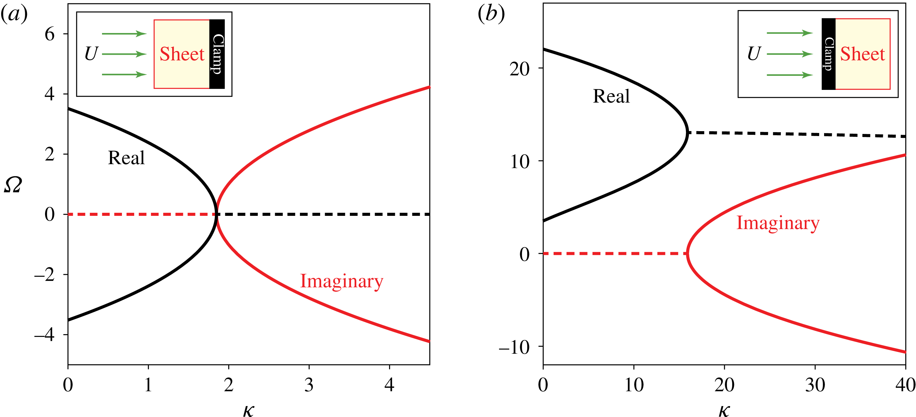
Figure 4 shows the calculated (complex) frequencies,
 ${\it\Omega}$
, for both the conventional and inverted flag problems, as a function of the dimensionless flow speed,
 ${\it\kappa}$
. Emergence of a non-zero imaginary component defines the onset of an instability (bifurcation), due to the time dependence,
 $\exp (-\text{i}{\it\Omega}t)$
(
 $t$
is dimensionless time, i is the imaginary unit), implicit in (3.2); see Kornecki et al. (Reference Kornecki, Dowell and O’Brien1976). While results for the conventional and inverted flags exhibit some obvious similarities, the striking difference is that the conventional flag problem (figure 4
b) bifurcates at non-zero frequency (see real part, at
 ${\it\kappa}=15.9$
), whereas stability of the inverted flag (figure 4
a) is lost at zero frequency when
 ${\it\kappa}=1.85$
(to three significant figures).
Drawing on the rationale in § 3.2.1 for use of Kornecki’s steady theory, the results in figure 4(a) prove that bifurcation, i.e. loss of stability, of the inverted flag’s zero-deflection equilibrium is a steady process (occurring at zero frequency) – it is therefore independent of the added mass parameter
 ${\it\mu}$
; this is compared to measurements in § 3.4.1. This finding contrasts to the conventional flag problem, with the results of figure 4(b) establishing that unsteady fluid loading can be important at bifurcation, i.e. the full unsteady theory of Kornecki et al. (Reference Kornecki, Dowell and O’Brien1976) should be used, which depends on
 ${\it\mu}$
. Indeed, it is well established that bifurcation of a conventional flag is strongly dependent on
 ${\it\mu}$
(Kornecki et al.
Reference Kornecki, Dowell and O’Brien1976; Shelley & Zhang Reference Shelley and Zhang2011).
Stability of the zero-deflection equilibrium, for (a) an inverted flag and (b) a conventional flag. Dimensionless frequency,
 ${\it\Omega}$
(3.2) versus dimensionless flow speed,
 ${\it\kappa}$
are shown. A positive imaginary component indicates an unstable equilibrium.

This analysis shows that, as the flow speed increases, the inverted flag of infinite aspect ratio becomes unstable at
 ${\it\kappa}=1.85$
due to the steady hydrodynamic lift force balancing the elastic restoring force of the sheet – higher speeds cause it to deflect from its zero-deflection equilibrium position. The inverted flag therefore exhibits a (buckling) divergence instability (Paidoussis et al.
Reference Paidoussis, Price and De Langre2010). The effect of this deflection on the sheet’s subsequent dynamics is explored in the § 4.
Next, we turn our attention to examining the effects of finite sheet aspect ratio,
 $H/L$
, on this instability.
3.3 Effect of finite aspect ratio on the divergence instability
In the previous section, we showed that the inverted flag’s zero-deflection equilibrium loses its stability through a steady fluid process. The effect of finite aspect ratio,
 $H/L$
, can therefore be calculated using inviscid theories for steady flow, which have been developed and utilised for wings of finite span (Anderson Reference Anderson1991).
We initially use Prandtl’s lifting-line theory, which strictly, is valid only for sheets of high aspect ratio. Nonetheless, lifting-line theory enables an asymptotic solution to be developed, and thus specification of the bifurcation point’s scaling behaviour as a function of aspect ratio. Accuracy of this (large aspect ratio) solution is then examined using the vortex lattice method. Because this numerical method is valid for sheets of arbitrary aspect ratio, it enables the range of validity of the lifting-line asymptotic solution to be quantified. As we shall see, this asymptotic solution works well over a broad range of aspect ratios.
3.3.1 Lifting-line theory
$(H/L\gg 1)$

A wing (of finite aspect ratio) in a steady flow generates edge vortices that reduce its overall lift. Lifting-line theory accounts for this effect by replacing the wing with an infinite set of horseshoe vortices, from which the overall lift is calculated. Some important conclusions from this theory are: (i) finite aspect ratio reduces the lift slope of the wing, i.e. the rate of change in lift with respect to its angle of attack, and (ii) the angle of attack for which there is no lift is unaffected by the wing’s aspect ratio.
Lifting-line theory requires calculation of the zero-lift angle of attack,
 ${\it\alpha}_{0}$
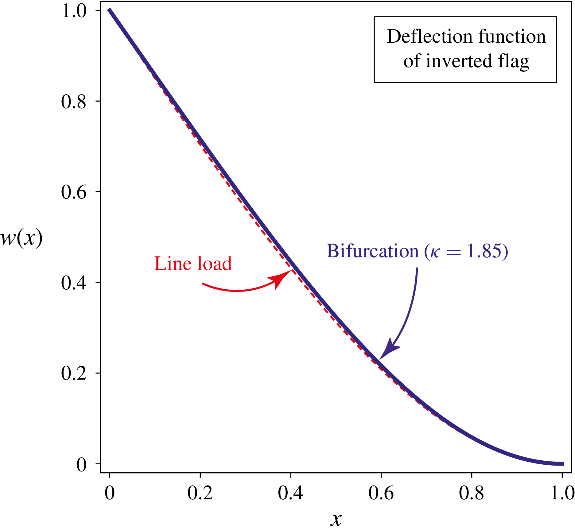
. This is obtained from the deflection function of the infinite aspect ratio sheet, which is specified at the bifurcation point by (3.6), see figure 5; it is calculated from the eigenvalue problem discussed in § 3.2. The deflection function at bifurcation closely resembles that due to a line load at the sheet’s free end; this is not surprising, because the pressure load is maximum at that position on the sheet where it exhibits a square root singularity. Its zero-lift angle of attack is given by
 $$\begin{eqnarray}{\it\alpha}_{0}=\frac{A}{{\rm\pi}L}\int _{0}^{{\rm\pi}}w^{\prime }({\it\zeta})(1+\cos {\it\phi})\,\text{d}{\it\phi}=-0.578\frac{A}{L},\end{eqnarray}$$
where
 $A$
is the sheet’s free end displacement; the deflection function
 $w$
is normalised by this value, see figure 5. Increasing the sheet’s displacement,
 $A$
, thus linearly decreases its zero-lift angle of attack.
Normalised deflection function (by its maximum value) for an inverted flag of infinite aspect ratio at its bifurcation point
 ${\it\kappa}=1.85$
(solid blue line), calculated using the theory of Kornecki et al. (Reference Kornecki, Dowell and O’Brien1976). Deflection function for a line load at the sheet’s free end (dashed red line), shown for comparison.

As discussed above,
 ${\it\alpha}_{0}$
is independent of the sheet’s aspect ratio,
 $H/L$
. Since the deflected sheet is at a geometric angle of attack of zero, lifting-line theory then establishes that its lift curve has (i) an identical slope to that of a flat sheet with an angle of attack
 ${\it\alpha}=0.578A/L$
, and (ii) a zero-lift angle of attack that is given by (3.7). The sheet has a rectangular geometry (planform), and thus dependence of its lift slope on its aspect ratio,
 $H/L$
, is given by the standard result from lifting-line theory (Anderson Reference Anderson1991):
 $$\begin{eqnarray}\frac{\text{d}C_{L}}{\text{d}{\it\alpha}}=\frac{2{\rm\pi}}{1+\displaystyle \frac{2L}{H}(1+{\it\tau})},\end{eqnarray}$$
where
 $C_{L}$
is the normalised lift coefficient, and
 ${\it\tau}\ll 1$
is the Glauert coefficient;
 ${\it\tau}$
is approximated to zero here.
Equations (3.7) and (3.8) completely specify the dependence of the hydrodynamic lift force on the sheet’s displacement,
 $A$
, at the bifurcation point. This assumes that the deflection function of the sheet at bifurcation is unaffected by its aspect ratio, to leading order for large aspect ratio; this is validated in the next section. Importantly,
 ${\it\kappa}$
is (proportional to) the ratio of the hydrodynamic lift force to the elastic restoring force of the sheet, both of which vary linearly with
 $A$
; as is evident from (3.1) and (3.2). It then follows that a reduction in the lift slope by a factor of
 $(1+2L/H)$
(see (3.8)), increases the critical value for
 ${\it\kappa}$
(at which bifurcation occurs) by the same factor, i.e. a higher flow velocity is required to achieve the same lift force.
As such, the critical value for
 ${\it\kappa}$
at which the zero-deflection equilibrium loses its stability is
 $$\begin{eqnarray}{\it\kappa}_{\mathit{lower}}\equiv {\it\rho}U_{\mathit{lower}}^{2}L^{3}/D\approx 1.85\left(1+\frac{2L}{H}\right).\end{eqnarray}$$
Since this result is formally valid for sheets of large aspect ratio (
 $H/L$
) only, we now examine the range of its validity by comparison to numerical results that hold for all aspect ratios – these are obtained using the vortex lattice method.
3.3.2 Vortex lattice method (arbitrary
$H/L$
)

The vortex lattice method (VLM) employs a vortex sheet whose strength varies over the planform of the wing. This generalises the methodology of lifting-line theory, enabling application to wings of arbitrary aspect ratio (Anderson Reference Anderson1991). As such, VLM is used here to assess the accuracy of (3.9) which is derived for large aspect ratio.
The small-deflection theory of thin plates is used in conjunction with VLM, to numerically calculate the value of
 ${\it\kappa}_{\mathit{lower}}$
as a function of aspect ratio. The governing equation for the (steady) dimensionless deflection function,
 $w$
, is (Landau & Lifshitz Reference Landau and Lifshitz1970)
 $$\begin{eqnarray}{\rm\nabla}^{4}w(x,z)={\it\kappa}p,\end{eqnarray}$$
where the dimensionless Cartesian spatial coordinates
 $(x,z)$
are scaled by the sheet’s length,
 $L$
, and the dimensionless pressure,
 $p$
, by
 ${\it\rho}U^{2}A/L$
.
Importantly, the deflection function
 $w$
is independent of the
 $z$
-coordinate (see figure 2) in the limit of infinite aspect ratio (Kornecki et al.
Reference Kornecki, Dowell and O’Brien1976). This also holds approximately for aspect ratios,
 $H/L$
, much smaller than unity, because the sheet then behaves as an Euler–Bernoulli beam (Landau & Lifshitz Reference Landau and Lifshitz1970). Since
 $w$
is independent of
 $z$
in these complementary limiting cases, we approximate the deflection function for all aspect ratios by one that is independent of
 $z$
; this is expected to produce a small error in
 ${\it\kappa}$
, by a factor less than
 $1-{\it\nu}^{2}$
(Sader & White Reference Sader and White1993). Multiplying both sides of (3.10) by
 $w$
, integrating over the sheet’s surface and utilising its boundary conditions, then gives
 $$\begin{eqnarray}{\it\kappa}=\frac{\displaystyle \int _{0}^{1}\left(\displaystyle \frac{\text{d}^{2}w}{\text{d}x^{2}}\right)^{2}\,\text{d}x}{\displaystyle \int _{0}^{1}p_{\mathit{ave}}w\,\text{d}x},\end{eqnarray}$$
where
 $p_{\mathit{ave}}$
is the spanwise-averaged pressure distribution, i.e. in the
 $z$
-direction. The average pressure,
 $p_{\mathit{ave}}$
, is linearly dependent on the deflection function
 $w$
(Anderson Reference Anderson1991), and hence
 ${\it\kappa}$
is independent of the displacement,
 $A$
, as required. Equation (3.11) is used to determine the critical value,
 ${\it\kappa}_{\mathit{lower}}$
, as a function of the sheet’s aspect ratio,
 $H/L$
.
We decouple the fluid-structure problem using a Rayleigh–Ritz approach, by expanding the deflection function:
 $$\begin{eqnarray}w=\mathop{\sum }_{m=2}^{M}b_{m}(1-x)^{m},\end{eqnarray}$$
which satisfies the clamp boundary condition for the inverted flag (at
 $x=1$
). The coefficients
 $b_{m}$
are to be determined for a fixed number of terms,
 $M$
, which is increased until convergence is reached.
Use of the series expansion in (3.12) enables the hydrodynamic pressure
 $p$
to be calculated a priori for each individual power-law deflection function,
 $w_{m}(x)=(1-x)^{m}$
. This is performed numerically using VLM (Tornado 2015). Due to linearity (above), the overall average pressure distribution
 $p_{\mathit{ave}}$
for the complete deflection function, from these individual contributions, is then immediately determined for arbitrary
 $b_{m}$
. This expression for the pressure is substituted into (3.11), and the unknown coefficients,
 $b_{m}$
, evaluated from its stationary solution. This Rayleigh–Ritz approach ensures that the resulting value for
 ${\it\kappa}_{\mathit{lower}}$
is a strict upper bound (Leissa Reference Leissa1969).
Because the deflection function for infinite aspect ratio is well approximated by that of an end-loaded cantilevered sheet (see figure 5), which is a simple cubic polynomial function, the general polynomial expansion in (3.12) is expected to converge rapidly. Indeed, use of three terms only (
 $M=4$
) in (3.12) is found to yield convergence of
 ${\it\kappa}_{\mathit{lower}}$
to better than 99 %. The number of panels in VLM is increased systematically until a convergence of greater than 95 % is achieved for each
 $w_{m}(x)$
; higher levels of convergence are limited by the significant memory requirements and available computational resources. Final values for
 ${\it\kappa}_{\mathit{lower}}$
are derived by extrapolating calculated results as a function of the number of VLM panels; these differ by
 ${<}$
5 % from values obtained using the largest number of panels.
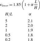
Results for
 ${\it\kappa}_{\mathit{lower}}$
, using this numerical approach, are given in table 1 as a function of aspect ratio,
 $H/L$
. These results establish the accuracy of (3.9), which is derived in the large aspect ratio limit. Indeed, the value of
 ${\it\alpha}=2.1$
for the largest aspect ratio studied,
 $H/L=5$
, is consistent with omission of the Glauert coefficient in (3.9), cf. (3.8) and (3.9). Glauert (Reference Glauert1926) reports a value of
 ${\it\tau}=0.16$
for
 $H/L=5$
, which decreases with a reduction in aspect ratio. While (3.9) is an asymptotic formula for large aspect ratio, the data in table 1 shows that it is also accurate for very small aspect ratio – the
 ${\it\alpha}$
-coefficient varies by
 ${\approx}$
10 % over the range of
 $H/L$
studied. Use of the deflection function derived from (3.2) for infinite aspect ratio (see figure 5), rather than the Rayleigh–Ritz approach, yields results for
 ${\it\kappa}_{\mathit{lower}}$
that only slightly overestimate those in table 1 (by a few percent).
Numerical results obtained using the Rayleigh–Ritz and vortex lattice methods, described in § 3.3.2. Results are presented using a generalisation of (3.9); formula given in first row. This shows that the sheet’s aspect ratio,
 $H/L$
, exerts a weak effect on the
 ${\it\alpha}$
-coefficient, validating the accuracy of (3.9).

For completeness, we note that identical results are obtained using an approach analogous to that in § 3.2. That is, solving the eigenvalue problem for the unsteady thin plate equation (i.e. including the solid inertia term omitted in (3.10)) with a steady hydrodynamic load (specified by VLM for each
 $w_{n}(x)$
in the above described Rayleigh–Ritz method), as a function of
 ${\it\kappa}$
. As expected, bifurcation is found to occur at zero frequency, i.e.
 ${\it\Omega}=0$
(data not shown). Omission of solid inertia in (3.10) exactly simplifies the analysis by enabling the direct evaluation of
 ${\it\kappa}_{\mathit{lower}}$
using (3.11).
3.3.3 Effect of finite Reynolds number
Measurements on wings at high Reynolds number show that the lift coefficient and its aspect ratio correction both decrease by a factor of between 0.855 and 0.875 (Higgins Reference Higgins1929; Pelletier & Mueller Reference Pelletier and Mueller2000) for the Reynolds number range considered here,
 $\mathit{Re}\approx 10^{4}{-}10^{5}$
, and for aspect ratios
 $H/L\geqslant 1$
. This establishes that viscosity exerts a small effect on the overall lift, provided the aspect ratio exceeds unity. Combining this observation with (3.9) yields the required theoretical result:
 $$\begin{eqnarray}{\it\kappa}_{\mathit{lower}}\approx 1.85\left(1+\frac{2L}{H}\right),\quad \frac{H}{L}\geqslant 1.\end{eqnarray}$$
Because the effects of viscosity have been shown to be small for aspect ratios greater than unity only, care must be taken when analysing measurements with
 $H/L<1$
. It is known that the sides of a wing generate vortices that can become trapped by the air flow and increase lift; the so-called ‘vortex-lift’ phenomenon (Anderson Reference Anderson1991). Since these trapped vortices occur at the sides of the wing, their effect on the overall lift is expected to increase with decreasing aspect ratio. These 3-D viscous effects are ignored in the 2-D inviscid calculations reported in the previous sections. Fully coupled Navier–Stokes-elastic simulations provide a rigorous approach for exploring such effects, but are hindered by the large Reynolds numbers used (
 $\mathit{Re}\approx 10^{4}{-}10^{5}$
). Numerical investigation provides an interesting avenue for further work, e.g. using the LES approach of Gilmanov et al. (Reference Gilmanov, Le and Sotiropoulos2015).
3.4 Comparison to measurement
We now compare predictions of the theory presented above to the measurements of (i) Kim et al. (Reference Kim, Cosse, Huertas Cerdeira and Gharib2013), and (ii) those reported in figure 3. We remind the reader that the experimental data in figure 3 extend the dataset presented in Kim et al. (Reference Kim, Cosse, Huertas Cerdeira and Gharib2013), by demonstrating the effect of changing the sheet’s aspect ratio.
3.4.1 Effect of the added mass parameter
${\it\mu}$

Experiments by Kim et al. (Reference Kim, Cosse, Huertas Cerdeira and Gharib2013) show that the inverted flag loses its stability and deflects from its zero-deflection equilibrium at values of
 ${\it\kappa}_{\mathit{lower}}$
that are similar for two fluids: air and water. Note that the dimensionless parameters
 ${\it\kappa}$
and
 ${\it\mu}$
used here, which are taken from Kornecki et al. (Reference Kornecki, Dowell and O’Brien1976), are reciprocals of the
 ${\it\beta}$
and
 ${\it\mu}$
parameters of Kim et al. (Reference Kim, Cosse, Huertas Cerdeira and Gharib2013), respectively. We shall refer only to the definitions in (3.1) throughout this article.
The values of
 ${\it\mu}$
for air and water differ by three orders of magnitude, due to the difference in fluid density. For the
 $L=30$
cm inverted flag reported by Kim et al. (Reference Kim, Cosse, Huertas Cerdeira and Gharib2013),
 ${\it\mu}=0.38$
(air) and
 ${\it\mu}=320$
(water), representing strong fluid loading. The observed similitude with respect to
 ${\it\kappa}_{\mathit{lower}}$
, for varying
 ${\it\mu}$
, led to speculation of a divergence instability, though a definite conclusion could not be drawn based on only two data points. The theoretical analysis presented in the preceding section is consistent with these measurements and now establishes that a divergence instability indeed occurs for all fluids (at high Reynolds numbers). As such, the critical dimensionless flow speed,
 ${\it\kappa}_{\mathit{lower}}$
, is independent of the surrounding fluid and hence
 ${\it\mu}$
; see (3.13).
3.4.2 Effect of the sheet’s aspect ratio,
$H/L$

The new measurements in figure 3, for the critical flow speed at which the zero-deflection equilibrium bifurcates as a function of aspect ratio, are used to assess the validity and accuracy of (3.13). As the flow speed is increased from zero, the sheet remains undeflected initially while exhibiting very small-amplitude fluctuations; see figure 3. At higher flow speeds, flapping motion is initiated and increases in amplitude rapidly over a narrow range of flow speeds. The required bifurcation point (for comparison with theory) is selected by the flow speed at which the flapping amplitude is approximately 50 % of its maximum value, in this (narrow) flow speed range; this is obtained by measuring the flow speeds at which the amplitude is 25 % and 75 % of this maximum value, and taking their average. This allows the bifurcation point and its uncertainty to be quantified.
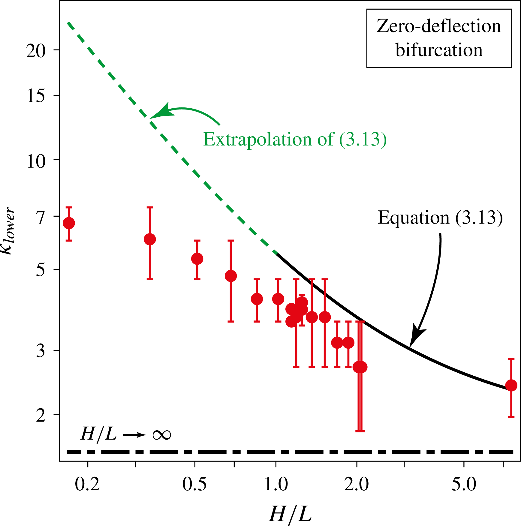
Figure 6 presents the results of this experimental analysis and a comparison to (3.13), for the aspect ratios measured; there are no adjustable parameters. Measurements in air on sheets of length 5.1 and 30 cm are used, dimensionless data from which are found to collapse precisely; see figure 6. This shows that the scaling parameters in (3.1) correctly capture the behaviour of this bifurcation phenomenon. We remind the reader that (3.13) holds for
 $H/L\geqslant 1$
only. Figure 6 shows that (3.13) correctly predicts the loss of stability of the zero-deflection equilibrium at high aspect ratio, with (slightly) decreasing accuracy as aspect ratio is reduced. The infinite aspect ratio result of
 ${\it\kappa}_{\mathit{lower}}=1.85$
strongly underestimates measurements of all the inverted flags studied here, which possess finite aspect ratios. This confirms the above theoretical consideration that the sides of the inverted flag reduce the hydrodynamic lift, requiring a higher flow speed for the sheet to become unstable. A general increase in
 ${\it\kappa}_{\mathit{lower}}$
with decreasing aspect ratio is predicted, and observed.
Bifurcation point of the zero-deflection equilibrium of an inverted flag, showing the critical dimensionless flow speed,
 ${\it\kappa}_{\mathit{lower}}$
, as a function of aspect ratio,
 $H/L$
. Comparison of measurements in air (red dots) using sheets of length 5.1 cm and 30 cm, with the large aspect ratio (
 $H/L\geqslant 1$
) formula (3.13) (solid black line). The asymptotic limit
 $H/L\rightarrow \infty$
is indicated (dash-dotted black line). The (extrapolated) prediction of (3.13) is also shown for
 $H/L<1$
(dashed green line); this lies outside its range of validity and is given for reference only.

For reference, in figure 6 we also show the (extrapolated) prediction of (3.13) for
 $H/L<1$
, which is strictly outside of its regime of validity. Interestingly, measurements are found to strongly underestimate this theoretical prediction. This deviation is consistent with the vortex-lift phenomenon, discussed in § 3.3.3, whose effect will become more pronounced with decreasing aspect ratio. Its presence would enhance the lift experienced by the sheet, reducing the critical flow speed
 ${\it\kappa}_{\mathit{lower}}$
required for bifurcation, as observed. This possibility will be explored in a future study.
This completes our analysis of the zero-deflection equilibrium’s stability (at low flow speed). The measurements in figure 3 show that when this equilibrium bifurcates, large-amplitude flapping is launched immediately. In the next section, we explore the mechanisms giving rise to this behaviour.
4 Large-amplitude flapping region
The divergence instability at
 ${\it\kappa}_{\mathit{lower}}$
causes the sheet to deflect spontaneously from its zero-deflection equilibrium. The sharp leading edge of the sheet is then presented at large angle of attack to the impinging flow, strongly modifying the fluid motion. While the flow over the sheet is attached for small angles of attack (see § 3.2), a large angle of attack leads to flow separation and periodic shedding of vortices from the deflected sheet’s concave surface (Schmitz Reference Schmitz1941). The resulting hydrodynamic load will periodically force the sheet, which can potentially lead to a VIV.
VIVs of elastic structures have been studied widely and are known to exhibit distinct characteristics (Bearman Reference Bearman1984; Blackburn & Henderson Reference Blackburn and Henderson1996; Williamson & Govardhan Reference Williamson and Govardhan2004; Gabbai & Benaroya Reference Gabbai and Benaroya2005; Can Kara, Stoesser & McSherry Reference Can Kara, Stoesser and Mcsherry2015). We draw on this existing literature, and combine it with detailed measurements and a scaling analysis, to test the hypothesis that flapping of an inverted flag is a VIV.
4.1 Observations from the literature
Flapping of an inverted flag does not occur in the slender aspect ratio limit, i.e.
 $H/L\ll 1$
; see figure 3. We therefore focus on cases of larger aspect ratio, where flapping exists, and study the literature for two-dimensional bluff bodies (corresponding to the infinite aspect ratio limit of the inverted flag).
4.1.1 Periodic vortex shedding from a bluff body
Periodic vortex shedding from bluff bodies has an extensive history of study (Mallock Reference Mallock1907; Bernard Reference Bernard1908; von Karman Reference von Karman1911, Reference von Karman1912; Fage & Johansen Reference Fage and Johansen1927; Schmitz Reference Schmitz1941; Roshko Reference Roshko1954; Bearman Reference Bearman1984; Knisely Reference Knisely1990), and the Strouhal number is used widely to characterise it. The Strouhal number corresponds physically to the ratio of a convective time scale for the impinging flow to the period of vortex shedding. It is (traditionally) defined
 $$\begin{eqnarray}\mathit{St}\equiv \frac{f_{\mathit{vs}}D}{U},\end{eqnarray}$$
where
 $f_{\mathit{vs}}$
is the vortex shedding frequency (in Hz),
 $D$
is a characteristic length scale for the bluff body and
 $U$
the free-stream speed of the impinging flow. Measurements show that this vortex shedding is characterised by
 $\mathit{St}\approx 0.2$
for a wide range of bluff bodies in the Reynolds number range of interest here (
 $\mathit{Re}\approx 10^{4}{-}10^{5}$
), provided
 $D$
is chosen to be the dimension of the 2-D bluff body projected in the flow direction (Roshko Reference Roshko1954; Knisely Reference Knisely1990). This includes circular cylinders, wedges and thin plates at finite angles of attack. The latter case is most relevant to this study, because it closely mimics the geometry of a deflected inverted flag. This measured value of
 $\mathit{St}\approx 0.2$
is not unexpected because it indicates that the time scale for periodic vortex shedding is identical to that for convection of the free-stream flow over the body; the more natural use of angular frequency
 ${\it\omega}_{\mathit{vs}}=2{\rm\pi}f_{\mathit{vs}}$
leads to a modified Strouhal number
 $\mathit{St}^{\ast }\equiv {\it\omega}_{\mathit{vs}}D/U\approx 1$
, highlighting this balance of time scales.
Vortex shedding from a thin flat plate is certainly not expected for small angles of attack, where the flow remains attached and is predominately inviscid; see § 3.2. Indeed, thin airfoil theory is found to accurately predict the measured lift slope of a thin plate for angles of attack
 ${\lesssim}10^{\circ }$
(Pelletier & Mueller Reference Pelletier and Mueller2000). This lack of vortex shedding for angles of attack
 ${\lesssim}10^{\circ }$
is confirmed by the measurements of Knisely (Reference Knisely1990). Both Knisely (Reference Knisely1990) and Pelletier & Mueller (Reference Pelletier and Mueller2000) consider flows with Reynolds numbers
 $\mathit{Re}\approx 10^{4}{-}10^{5}$
, similar to the inverted flags here. Knisely (Reference Knisely1990) also shows that
 $\mathit{St}\approx 0.15$
for all angles of attack greater than
 ${\approx}10^{\circ }$
; simulations verify these observations (Lam & Wei Reference Lam and Wei2010). We use these observed properties of a thin plate in our analysis of the flapping motion of an inverted flag in § 4.2.
4.1.2 Frequency lock-in during a VIV
Discussion in the previous section focuses on periodic vortex shedding from rigid bluff bodies. If the bluff body is elastic, the periodic hydrodynamic force applied by the same vortex shedding can induce a vibration of the body. A primary characteristic of the VIV of an elastic bluff body, is synchronisation of its motion with this periodic vortex shedding.
Measurements on a wide range of structures show that increasing the flow velocity from zero leads to distinct behaviour over a finite band of velocities (Brika & Laneville Reference Brika and Laneville1993; Williamson & Govardhan Reference Williamson and Govardhan2004; Gabbai & Benaroya Reference Gabbai and Benaroya2005), which we now summarise. This behaviour is again characterised by the Strouhal number,
 $\mathit{St}$
, which sets the natural frequency,
 $f_{\mathit{vs}}$
, for periodic vortex shedding; see § 4.1.1. Two cases are often considered in the literature: light and heavy fluid loading. In the context of (3.1), these cases correspond to
 ${\it\mu}\ll 1$
and
 ${\it\mu}\gtrsim O(1)$
, respectively; see note below for clarification of these regimes in existing literature measurements of VIVs.
Light fluid loading. Increasing the flow velocity from zero increases the vortex shedding frequency,
 $f_{\mathit{vs}}$
, at constant Strouhal number, typically
 $\mathit{St}\approx 0.2$
; see § 4.1.1. When
 $f_{\mathit{vs}}$
is close to the natural resonant frequency of the elastic body,
 $f_{\mathit{res}}$
, the linear increase in
 $f_{\mathit{vs}}$
with flow speed ceases and the elastic body starts to vibrate at (or close to) its natural resonant frequency, with finite amplitude. Increasing the flow speed further does not alter this vibration frequency, with
 $f_{\mathit{vs}}\approx f_{\mathit{res}}$
, i.e. the vortex shedding frequency now departs from the
 $\mathit{St}\approx 0.2$
behaviour and
 $\mathit{St}$
decreases systematically. At higher flow speeds, where the Strouhal number is significantly lower than
 $\mathit{St}\approx 0.2$
, lock-in of
 $f_{\mathit{vs}}$
with
 $f_{\mathit{res}}$
is lost. The vortex shedding frequency returns to its previous behaviour, again satisfying
 $\mathit{St}\approx 0.2$
, and the oscillation amplitude drops dramatically.
Heavy fluid loading. The natural resonant frequencies of an elastic body in the presence and absence of fluid now differ considerably. For zero flow velocity,
 $f_{\mathit{res}}$
is significantly lower than its value when the fluid is absent, due to the strong inertial load exerted by the fluid that increases the body’s effective mass (Lindholm et al.
Reference Lindholm, Kana, Chu and Abramson1965; Sader Reference Sader1998). Importantly,
 $f_{\mathit{res}}$
depends on the flow velocity and the body’s oscillation amplitude, which can both have a significant effect. As such, the lock-in observed for light fluid loading is modified with the vortex shedding frequency no longer being constant during a VIV (Gabbai & Benaroya Reference Gabbai and Benaroya2005).
The above mentioned Strouhal number trends are insensitive to Reynolds number for the range under consideration here, i.e.
 $\mathit{Re}\approx 10^{4}{-}10^{5}$
(Knisely Reference Knisely1990; Williamson & Govardhan Reference Williamson and Govardhan2004; Gabbai & Benaroya Reference Gabbai and Benaroya2005).
Note on existing literature measurements of VIVs. It is important to emphasise that measurements of heavy fluid loading in the literature typically refer to cases where
 ${\it\mu}\sim O(1)$
with
 ${\it\mu}<1$
(Williamson & Govardhan Reference Williamson and Govardhan2004; Gabbai & Benaroya Reference Gabbai and Benaroya2005). This is to be compared to the inverted flags considered here, that exhibit added mass parameters of
 ${\it\mu}=0.38$
for air and
 ${\it\mu}=320$
for water (Kim et al.
Reference Kim, Cosse, Huertas Cerdeira and Gharib2013). These values of
 ${\it\mu}$
establish that the surrounding fluid significantly modifies the sheet’s resonant frequency in all measurements. Critically, measurements with
 ${\it\mu}>1$
have not been explored previously in the VIV literature, to the authors’ knowledge. The large values,
 ${\it\mu}\gg 1$
, for the inverted flag in water arise from the thin geometry of the sheet, whereas most VIV studies focus on circular cylinders (that naturally yield
 ${\it\mu}<1$
due to the difference in densities between solids and liquids), cf. added mass parameters of a circular cylinder and a flat rectangular sheet:
 $1/m^{\ast }$
in the Appendix of Williamson & Govardhan (Reference Williamson and Govardhan2004) and
 ${\it\mu}$
in (3.1), respectively. Note that the added mass parameter used in the literature is commonly
 $m^{\ast }$
(Williamson & Govardhan Reference Williamson and Govardhan2004), defining the ratio of inertia in the elastic body relative to that in the fluid, which is the reciprocal of
 ${\it\mu}$
(Kornecki et al.
Reference Kornecki, Dowell and O’Brien1976).
4.1.3 Effect of damping on a VIV
Damping is known to strongly modify the characteristics of a VIV (Khalak & Williamson Reference Khalak and Williamson1999; Williamson & Govardhan Reference Williamson and Govardhan2004; Gabbai & Benaroya Reference Gabbai and Benaroya2005). Specifically, increasing damping in the system reduces the maximum amplitude of a VIV, and the flow velocity range over which it occurs. This property is illustrated in figure 6 of Gabbai & Benaroya (Reference Gabbai and Benaroya2005), where a comparison of measurements on elastic circular cylinders immersed in both air and water, is provided. The limit of high damping has been shown to reduce the amplitude of a VIV to zero, i.e. the VIV is eliminated (Khalak & Williamson Reference Khalak and Williamson1999).
Measurements of inverted flags are available in both air (figure 3) and water (Kim et al. Reference Kim, Cosse, Huertas Cerdeira and Gharib2013), allowing the effect of damping on the observed flapping to be assessed. In the next section, we shall also explore the effect of introducing additional damping to the inverted flag to see if it can eliminate flapping, in line with the above observation for a VIV (of an elastic cylinder).
Detailed measurements of the inverted flag’s dynamics are now presented to test for these signatures of a VIV, thus enabling an assessment of the hypothesis that flapping is a VIV.
4.2 Inverted-flag measurements
We begin by exploring the effect of damping on the behaviour of the inverted flag in the flapping region.
4.2.1 Effect of additional damping
In § 3 we showed that the sheet’s zero-deflection equilibrium is unstable for normalised flow speeds greater than
 ${\it\kappa}_{\mathit{lower}}$
, because the sheet’s hydrodynamic lift (at small angle of attack) exceeds its elastic restoring force. This causes the sheet to deflect spontaneously from its zero-deflection equilibrium, leading to flow separation – which decreases the sheet’s lift slope and enhances its drag (Anderson Reference Anderson1991). This reduction in hydrodynamic lift limits the sheet’s deflection, which can in principle now reach a new finite-deflection equilibrium as the flow speed is increased immediately past
 ${\it\kappa}_{\mathit{lower}}$
. However, such an equilibrium is not observed in the measurements reported in figure 3 or by Kim et al. (Reference Kim, Cosse, Huertas Cerdeira and Gharib2013).
This prediction of a new (finite-deflection) equilibrium implicitly assumes that the hydrodynamic lift (and drag) are steady, which is not the case; periodic vortex shedding is always present, see § 4.1.1. As such, the above discussion of lift reduction refers to lift in a time-averaged sense. Importantly, the effects of such periodic forcing (superimposed on this average lift) can be reduced through the introduction of additional damping. This basic mechanism is highlighted in the literature, where damping has been shown to reduce the amplitude of a VIV and ultimately eliminate it; see § 4.1.3.
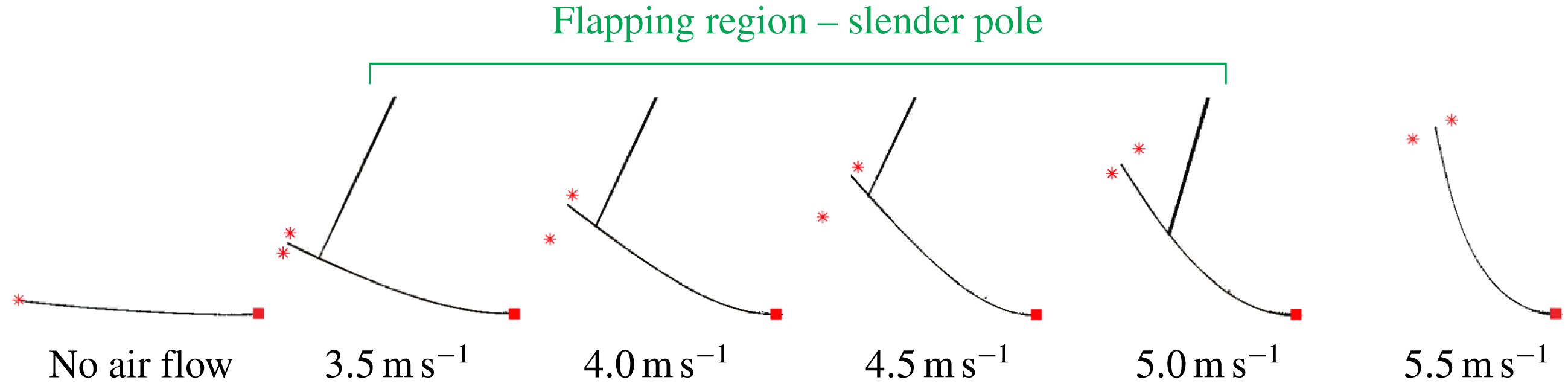
To test for the existence of this new equilibrium deflection, we introduce additional damping by lightly touching the inverted flag with a slender rigid pole; this takes kinetic energy away from the sheet when it oscillates. Figure 7 shows the results of these measurements over the complete range of air flow speeds studied, including the flapping region (highlighted). The pole is found to eliminate flapping and a new stable equilibrium is indeed observed in the flapping region; a restoring force is discovered when the pole is present, that drives the sheet to a previously unobserved stable finite-deflection equilibrium. The pole does not restrict motion of the sheet in both directions, but is applied on one side only – its effect is therefore to damp the motion rather than induce a stable equilibrium, which is illustrated in the following discussion.
Measurements showing the effect of additional damping in the flapping region. New stable equilibrium in the flapping region (air flow speeds shown here:
 $3.5{-}5~\text{m}~\text{s}^{-1}$
) is observed when a mechanically detached slender pole is introduced. At lower or higher flow speeds, the slender pole is not required because a stable equilibrium already exists, and introducing it has no effect. Asterisks indicate the range of motion observed in each measurement, which is predominantly due to twisting of the sheet; see movie in supplementary materials. This twisting motion may be due to the three-dimensional nature of the flow over the sheet. Sheet properties (
 $L=30$
cm,
 $H=62$
cm).

A movie showing the effects of the pole is given in the supplementary materials available online at http://dx.doi.org/10.1017/jfm.2016.139 (the
 $3.5~\text{m}~\text{s}^{-1}$
image in figure 7 is taken from this movie). Strikingly, the sheet does not move from this new equilibrium once the pole is first removed, highlighting its inherent stability. Nonetheless, the sheet does start oscillating back and forth with increasing amplitude, and flapping motion is reinitiated in finite time. This shows that unsteady forces are responsible for the sheet’s instability – additional damping (induced by the pole) is required for the existence of the new stable equilibrium. Figure 7 shows that the magnitude of this new equilibrium deflection monotonically increases with flow speed and smoothly transitions into the (previously observed) deflected equilibrium above the flapping region (reported in figure 3). In this latter region, the pole has no effect on the equilibrium deflection. This measurement is in line with the above discussion regarding the effects of flow separation on the average lift, since increasing the flow speed will increase this lift and thus the sheet’s deflection. It also shows that flow unsteadiness causes flapping of the inverted flag.
The results in figure 7 are therefore in accordance with the known effect of damping on the elimination of a VIV (discussed in § 4.1.3).
4.2.2 Effect of changing the surrounding fluid
In the previous section, we showed that strongly increasing the damping by external means (using a slender pole) stops the inverted flag from flapping and gives rise to a new stable equilibrium. If flapping is indeed a VIV, then changing the fluid from air to water is again expected to impact its dynamics because this also changes the damping.
Measurements in water by Kim et al. (Reference Kim, Cosse, Huertas Cerdeira and Gharib2013) are used for this purpose and show that the inverted flag’s flapping dynamics are modified significantly relative to air. Namely, the onset of flapping at low flow speed, i.e.
 ${\it\kappa}_{\mathit{lower}}$
, is similar to air (as noted in § 3.4.1), but the speed
 ${\it\kappa}_{\mathit{upper}}$
at which flapping ceases abruptly and a stable large-deflection equilibrium emerges, decreases by a factor of two. As such, the flow speed range over which flapping is observed is smaller in water, in comparison to air. Moreover, measurements in water show that as the flow speed increases, the onset of flapping at
 ${\it\kappa}_{\mathit{lower}}$
occurs at a greatly reduced amplitude relative to operation in air. The amplitude is enhanced with increasing flow speed, but is smaller than measurements in air, cf. figures 2 and 4 of Kim et al. (Reference Kim, Cosse, Huertas Cerdeira and Gharib2013); note that an inverse flow speed,
 ${\it\beta}\equiv 1/{\it\kappa}$
, is used in that study. Operation in water is found to restrict the motion in many cases, particularly at low flow speeds, with the sheet not crossing its zero-deflection position during an oscillation, i.e. flapping only occurs on one side with reduced amplitude (Kim et al.
Reference Kim, Cosse, Huertas Cerdeira and Gharib2013).
These observations are similar to known properties of a VIV, where an increase in damping reduces (i) the oscillation amplitude of a VIV, and (ii) the flow speed range over which it occurs; see § 4.1.3.
4.2.3 Synchronisation of flapping motion with vortex shedding
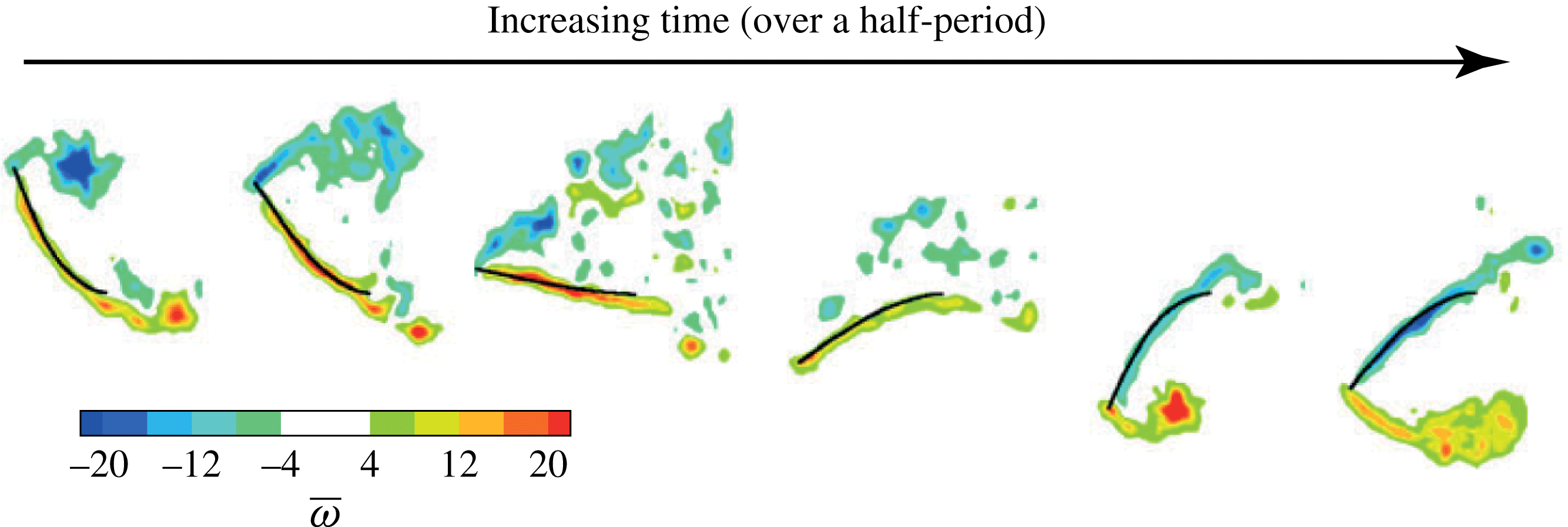
A key attribute of a VIV is the synchronisation of vortex shedding from the elastic body with the body’s motion. Kim et al. (Reference Kim, Cosse, Huertas Cerdeira and Gharib2013) provided flow visualisation measurements of an inverted flag flapping in water. These measurements are reproduced in figure 8, showing the motion of the sheet over a half-period of the flapping oscillation. These measurements clearly demonstrate that the formation and subsequent shedding of vortices from the leading (and trailing) edges of the sheet are synchronised with the sheet’s motion, as required. This experimental observation is also confirmed by recent computational simulations of the inverted flag, using an LES approach to capture the high Reynolds numbers involved (Gilmanov et al. Reference Gilmanov, Le and Sotiropoulos2015).
Sequential vortex formation process from an inverted flag undergoing flapping in water. Non-dimensional vorticity contours are indicated:
 $\overline{{\it\omega}}={\it\omega}_{\mathit{vs}}L/U$
, where
 ${\it\omega}_{\mathit{vs}}$
is the vorticity (not to be confused with the angular frequency,
 ${\it\omega}$
). Measurements taken from figure 6(a) of Kim et al. (Reference Kim, Cosse, Huertas Cerdeira and Gharib2013).

4.2.4 Strouhal number of flapping
Vortex-induced vibrations are initiated typically at a Strouhal number of
 $\mathit{St}\approx 0.2$
. Here, we explore the dynamics of the inverted flag in the flapping region to see if it also exhibits this behaviour. Example measurements are shown for an inverted flag with
 $L=5.1$
cm and
 $H=6.4$
cm, while noting that similar behaviour is observed for other aspect ratios and length.
The flapping frequency is obtained from stroboscopic images of the sheet, which are digitised to yield time series of its displacement. Deflections of the sheet’s free end in both the
 $x$
- and
 $y$
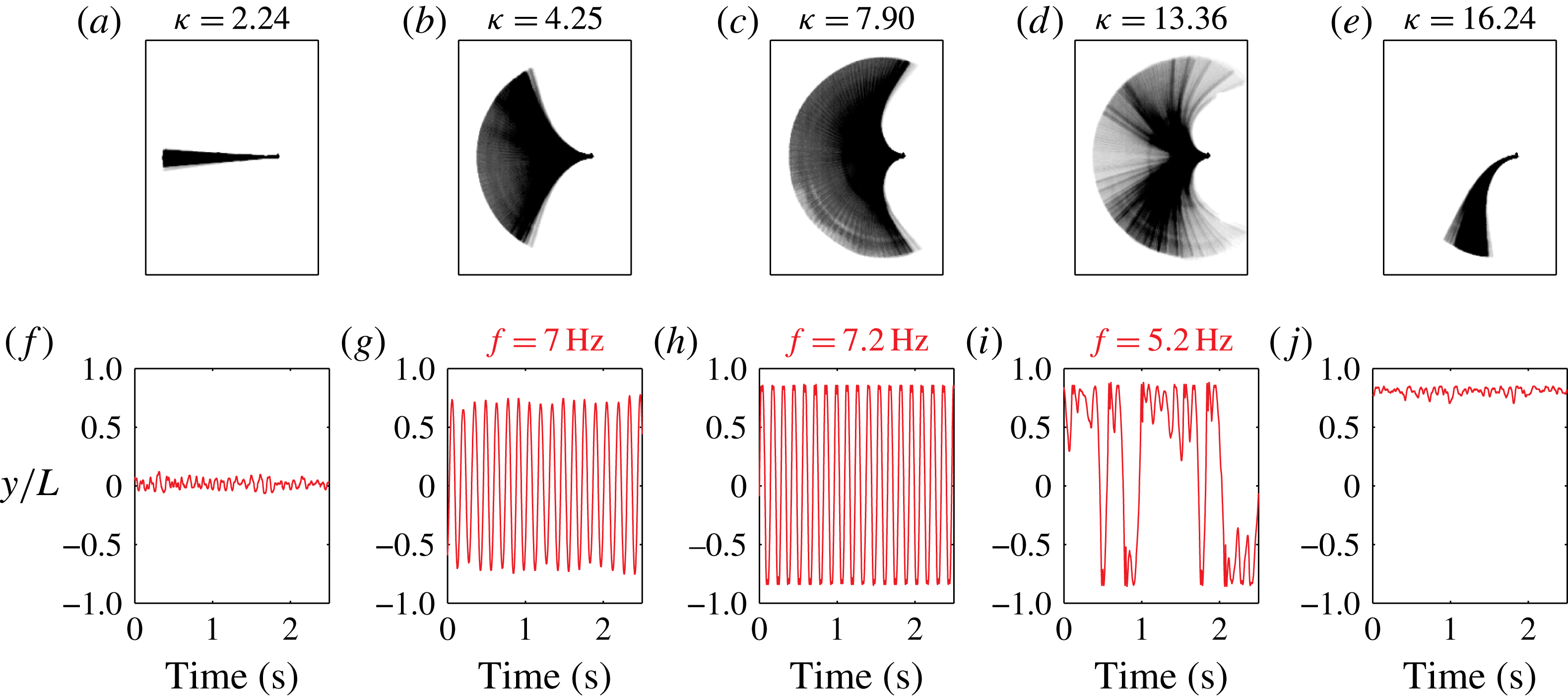
-directions are measured; see figure 2 for coordinate system. Figure 9 presents a sample of these stroboscopic images and their corresponding time series (for the
 $y$
-component only; the
 $x$
-component exhibits similar behaviour), as a function of
 ${\it\kappa}$
. Data at low flow speed in the flapping region clearly show that the sheet’s motion is highly periodic; this data is discussed further in § 4.2.7. The time series data is Fourier transformed to yield the required flapping frequency,
 $f_{\mathit{res}}$
, which is selected to be the spectral component of largest magnitude. These measured values for
 $f_{\mathit{res}}$
are shown in figure 9, for three values of
 ${\it\kappa}$
within the flapping region.
Stroboscopic images (a–e) and corresponding times series (f–j) of the sheet’s motion (directly below), as a function of
 ${\it\kappa}$
. The
 $y$
-coordinate listed is the position of the sheet’s free end; see figure 2. The flapping frequency as a function of
 ${\it\kappa}$
is also indicated. Sheet with
 $L=5.1~\text{cm}$
and
 $H=6.4~\text{cm}$
, measured in air.

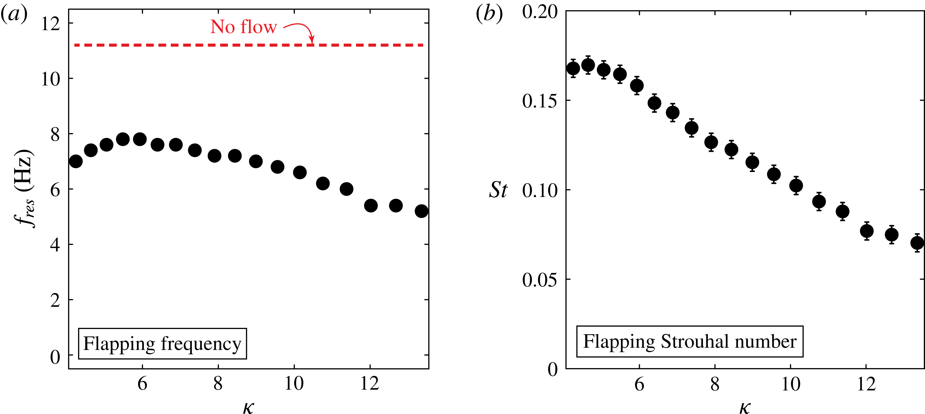
Figure 10(a) gives the complete dataset for
 $f_{\mathit{res}}$
, over all values of
 ${\it\kappa}$
measured in the flapping region, i.e. for
 ${\it\kappa}>{\it\kappa}_{\mathit{lower}}$
. This shows that the flapping frequency,
 $f_{\mathit{res}}$
, varies slightly with flow speed, but is significantly lower than the natural resonant frequency of the sheet in a quiescent fluid. As discussed in § 4.1.2, the resonant frequency of an elastic structure under heavy fluid loading depends on (i) the added mass parameter,
 ${\it\mu}$
, (ii) the flow speed and (iii) its oscillation amplitude. The observations in figure 10(a) are therefore in line with this expectation, because the fluid loading is strong (
 ${\it\mu}=0.38$
). Moreover, we observe that the maximum flapping frequency,
 $f_{\mathit{res}}\approx 8~\text{Hz}$
at
 ${\it\kappa}\approx 6$
, coincides with the sheet exhibiting a maximum deflection oriented
 $90^{\circ }$
to the flow direction – illustrating the connection between the flapping amplitude (and shape of the vibrating mode) with
 $f_{\mathit{res}}$
.
Flapping dynamics of the inverted flag studied in figure 9. (a) Flapping frequency,
 $f_{\mathit{res}}$
, and (b) Strouhal number,
 $St$
.

Corresponding results for the Strouhal number of the inverted flag are provided in figure 10(b). In accordance with (4.1), the Strouhal number for an inverted flag is defined (Kim et al. Reference Kim, Cosse, Huertas Cerdeira and Gharib2013)
 $$\begin{eqnarray}\mathit{St}\equiv \frac{f_{\mathit{res}}A}{U},\end{eqnarray}$$
where
 $f_{\mathit{res}}$
is the flapping (resonant) frequency and
 $A$
is the maximum amplitude of flapping (peak-to-peak in the
 $y$
-direction; see figure 2) to account for the deformable geometry of the flapping sheet and allow for comparison to previous studies on other bodies. Strikingly, the data in figure 10(b) shows that flapping is initiated at
 $\mathit{St}\approx 0.15$
, with the Strouhal number decreasing systematically as the flow speed increases – flapping ceases when the Strouhal number is below half its initial value.
These values for
 $St$
are quantitatively similar to those reported previously (Kim et al.
Reference Kim, Cosse, Huertas Cerdeira and Gharib2013) for inverted flags made from the (larger) sheet of length
 $L=30$
cm. The sheet length-to-thickness ratio is identical for both inverted-flag sizes,
 $L=5.1$
and 30 cm, and therefore, the flow speed where flapping begins is identical in both cases; see (3.1). As such, the Reynolds number for the
 $L=30$
cm flag studied by Kim et al. (Reference Kim, Cosse, Huertas Cerdeira and Gharib2013) is six times larger than for the
 $L=5.1$
cm flag reported in figures 9 and 10, while their dynamics occur at the same
 ${\it\kappa}$
and
 ${\it\mu}$
values. The
 $L=5.1$
and 30 cm flags therefore probe different flow regimes. This quantitative behaviour of the Strouhal number with increasing flow speed, and its insensitivity to Reynolds number, are identical to observations of VIVs of a broad range of mechanical structures; see § 4.1.2. The low Reynolds number computational simulations of inverted flag flapping by Ryu et al. (Reference Ryu, Park, Kim and Sung2015) exhibit similar behaviour, even though the Reynolds numbers are two orders of magnitude smaller.
Flapping in water (figure 4a of Kim et al. (Reference Kim, Cosse, Huertas Cerdeira and Gharib2013)) is somewhat different to air because the sheet does not always exhibit (the same qualitative) side to side oscillations, but instead flaps on one side predominantly – this modified mode shape leads to a reduction in amplitude and hence Strouhal number; see § 4.2.2.
4.2.5 Can a VIV be launched at
${\it\kappa}_{\mathit{lower}}$
?

Next, we examine whether it is possible for a VIV to be launched immediately following the divergence instability at
 ${\it\kappa}_{\mathit{lower}}$
. This is performed using a scaling analysis of the motion under the stated hypothesis that flapping is a VIV. This is motivated by the experimental observation that flapping starts immediately at
 ${\it\kappa}_{\mathit{lower}}$
; see figure 3.
The resonant frequency of a 2-D cantilevered sheet, in the absence of fluid, is (Looker & Sader Reference Looker and Sader2008)
 $$\begin{eqnarray}f_{\mathit{res}}=\frac{C_{1}^{2}}{2{\rm\pi}L^{2}}\sqrt{\frac{D}{{\it\rho}_{s}h}},\end{eqnarray}$$
where
 $C_{1}=1.8751$
(for the fundamental flexural mode). Immersion in fluid increases the effective mass of the sheet, due to the fluid’s inertial load, and thus lowers the sheet’s resonant frequency. This increase in mass is accounted for by replacing the areal mass density
 ${\it\rho}_{s}h$
with
 ${\it\rho}_{s}h(1+a{\it\mu})$
(Lindholm et al.
Reference Lindholm, Kana, Chu and Abramson1965), where
 $a$
is an order one coefficient, which for simplicity we approximate by
 $a\approx 1$
. This gives the required expression for the resonant frequency of the sheet in fluid:
 $$\begin{eqnarray}f_{\mathit{res}}\approx \frac{C_{1}^{2}}{2{\rm\pi}L^{2}}\sqrt{\frac{D}{{\it\rho}_{s}h(1+{\it\mu})}}.\end{eqnarray}$$
Substituting (4.4) into (4.2), and making use of (3.1), then gives
 $$\begin{eqnarray}{\it\kappa}\approx \frac{{\it\mu}}{3\,\mathit{St}^{2}(1+{\it\mu})}\left(\frac{A}{L}\right)^{2},\end{eqnarray}$$
defining the connection between the Strouhal number for flapping,
 $St$
, and the dimensionless flow speed,
 ${\it\kappa}$
. Equation (4.5) predicts
 $\mathit{St}\sim 1/\sqrt{{\it\kappa}}$
for constant
 $A/L$
and
 ${\it\mu}$
. This decreasing behaviour in
 $St$
is observed in figure 10(b) for larger values of
 ${\it\kappa}$
, where
 $A/L$
is approximately constant. We refrain from further direct comparison with (4.5), because the resonant frequency,
 $f_{\mathit{res}}$
, and hence the influence of the added mass parameter,
 ${\it\mu}$
, depend on
 ${\it\kappa}$
(see figure 10
a), an effect that has not been calculated.
We now specify the minimum and maximum values for the flapping amplitude,
 $A$
. The minimum limit for
 $A$
is set by the requirement that periodic vortex shedding must exist for a VIV to be launched. As discussed in § 4.1.1, the sheet must present a finite deflection that exceeds a minimum angle of attack for flow separation and periodic vortex shedding to occur. Using the measured value for a flat plate of
 ${\approx}10^{\circ }$
(Knisely Reference Knisely1990), as an approximation, gives the required lower limit for the flapping amplitude:
 $$\begin{eqnarray}\left.\frac{A}{L}\right|_{\mathit{min}}\approx 2\times \frac{{\rm\pi}}{180}\times 10^{\circ }\approx \frac{1}{3}.\end{eqnarray}$$
Existence of a minimum amplitude is clearly observed in the inverted-flag measurements reported in figure 3, and (4.6) agrees with minimum values for the flapping amplitude in figures 2 and 4 of Kim et al. (Reference Kim, Cosse, Huertas Cerdeira and Gharib2013).
The maximum flapping amplitude of an inverted flag is limited by its geometry: amplitudes greater than twice the sheet length are not physically realisable, i.e.
 $$\begin{eqnarray}\left.\frac{A}{L}\right|_{\mathit{max}}\approx 2.\end{eqnarray}$$
Substituting (4.6) and (4.7) into (4.5) gives
 $$\begin{eqnarray}\frac{{\it\mu}}{30\,\mathit{St}^{2}(1+{\it\mu})}\lesssim {\it\kappa}\lesssim \frac{4{\it\mu}}{3\,\mathit{St}^{2}(1+{\it\mu})}.\end{eqnarray}$$
Finally, we note that VIVs occur over the approximate range
 $\mathit{St}\in (0.1,0.2)$
for a wide range of bluff bodies; see § 4.1.2. Substituting these approximate upper and lower limits for
 $St$
into (4.8), gives the required inequality
 $$\begin{eqnarray}\frac{{\it\mu}}{1+{\it\mu}}\lesssim {\it\kappa}\lesssim \frac{100{\it\mu}}{1+{\it\mu}},\end{eqnarray}$$
which specifies the range of dimensionless flow speeds,
 ${\it\kappa}$
, for which a VIV can exist. Values of
 ${\it\kappa}$
outside this range require amplitudes that are either not possible geometrically (above the upper limit of this inequality), or do not allow the inverted flag to exhibit periodic vortex shedding (below the lower limit).
The added mass parameter for the inverted flags studied in figure 3 (in air) is
 ${\it\mu}=0.38$
, and thus (4.9) becomes
 $$\begin{eqnarray}0.3\lesssim {\it\kappa}\lesssim 30.\end{eqnarray}$$
Comparing this inequality with (3.13) (and the data in figure 6) shows that
 ${\it\kappa}_{\mathit{lower}}$
lies within the required flow speed range where a VIV can exist. This finding also holds true for inverted flags immersed in water, corresponding to
 ${\it\mu}\gg 1$
. We therefore conclude that a VIV can indeed be launched at
 ${\it\kappa}_{\mathit{lower}}$
, for the measurements presented.
Light fluid loading. Importantly, (3.13) does not satisfy (4.9) for light fluid loading, i.e.
 ${\it\mu}\ll 1$
, showing that an inverted flag cannot undergo a VIV in such cases: (i)
 ${\it\kappa}_{\mathit{lower}}>1.85$
, (ii)
 ${\it\kappa}_{\mathit{lower}}$
is independent of
 ${\it\mu}$
, and (iii) both the upper and lower limits of (4.9) approach zero as
 ${\it\mu}\rightarrow 0$
. The critical flow speed,
 ${\it\kappa}_{\mathit{lower}}$
, therefore lies outside of the required range for a VIV in (4.9) and an allowable oscillation amplitude does not exist, for very small
 ${\it\mu}$
. Physically, this is because the resonant frequency of the inverted flag,
 $f_{\mathit{res}}$
, under light fluid loading is significantly lower than the vortex shedding frequency,
 $f_{\mathit{vs}}$
, at
 ${\it\kappa}_{\mathit{lower}}$
– increasing the flow speed above
 ${\it\kappa}_{\mathit{lower}}$
, enhances
 $f_{\mathit{vs}}$
and thus eliminates the possibility of lock-in at any flow speed. Note that
 $f_{\mathit{res}}$
is independent of flow speed for
 ${\it\mu}\ll 1$
.
4.2.6 Is flapping a vortex-induced vibration?
We now summarise the above observations and analyses of an inverted flag’s dynamics:
-
(1) Flapping occurs for Strouhal numbers over the approximate range
$\mathit{St}\in (0.1,0.2)$
. It is initiated at a Strouhal number,
$\mathit{St}\approx 0.2$
, which decreases systematically with increasing flow speed. Flapping ceases when the Strouhal number is less than approximately half of its initial value. -
(2) The Strouhal number dependence on flow speed is insensitive to Reynolds number, as also observed for VIVs (see § 4.1.2). For the inverted flags studied, it does not change when the Reynolds number is varied by a factor of six.
-
(3) Periodic vortex shedding from the inverted flag always occurs after its divergence instability – due to the inverted flag presenting its sharp leading edge at large angle of attack to the impinging flow.
-
(4) Flapping is observed to occur above a minimum amplitude (see Kim et al. (Reference Kim, Cosse, Huertas Cerdeira and Gharib2013) and figure 3), as predicted by (4.6) – this is the regime where flow separation and periodic vortex shedding exist (Knisely Reference Knisely1990; Pelletier & Mueller Reference Pelletier and Mueller2000).
-
(5) The inverted flags studied here and by Kim et al. (Reference Kim, Cosse, Huertas Cerdeira and Gharib2013) operate under heavy fluid loading, i.e.
${\it\mu}\gtrsim O(1)$
. The flapping frequency depends on the surrounding fluid, varying with the flow speed and the flapping amplitude – as expected for the resonant frequency of elastic structures under heavy fluid loading. -
(6) Changing the damping experienced by the inverted flag modifies its dynamics, also in accordance with what is expected for a VIV:
-
(i) The amplitude of flapping and the flow speed range over which it occurs are reduced as damping increases. Namely, (a) the value of
${\it\kappa}_{\mathit{lower}}$
where flapping starts at low flow speed is unchanged when air or water is used, and (b) the upper value of
${\it\kappa}$
where flapping ceases is reduced by a factor of two in water, relative to air, and the flapping amplitude is smaller. -
(ii) Application of strong damping, to suppress the effects of unsteady hydrodynamic forces, eliminates flapping and leads to emergence of a new stable finite-deflection equilibrium. Flapping re-emerges once this damping is removed, showing that unsteady fluid forces are responsible for flapping.
-
-
(7) A scaling analysis shows that a VIV can be immediately launched following the divergence instability at
${\it\kappa}_{\mathit{lower}}$
, provided the inverted flag operates under heavy fluid loading; all inverted flags studied here satisfy this criterion. Operation under light fluid loading suppresses flapping. -
(8) Periodic vortex shedding from the leading and trailing edges of the inverted flag is synchronised with its flapping motion.


VIVs of elastic bluff bodies reported in the literature exhibit the same above-mentioned characteristics (for flapping of an inverted flag). This multifaceted connection therefore provides considerable evidence to support the hypothesis that flapping of an inverted flag is indeed a VIV. It is initiated by periodic vortex shedding from the sharp leading edge of the inverted flag at large angle of attack – which occurs when the inverted flag exhibits a divergence instability and deflects.
4.2.7 Transition to chaos
Simulations and measurements of conventional flags show that their dynamics can exhibit a transition to chaos as the sheet’s bending rigidity is reduced, or equivalently the flow speed is increased (Connell & Yue Reference Connell and Yue2007; Alben & Shelley Reference Alben and Shelley2008; Michelin et al. Reference Michelin, Llewellyn Smith and Glover2008; Ait Abderrahmane et al. Reference Ait Abderrahmane, Paidoussis, Fayed and Ng2012; Chen et al. Reference Chen, Jia, Wu, Yin and Ma2014). In this section, we examine the possibility that chaos also occurs in the flapping region of an inverted flag.
The measurements in figure 9(f–j) show that flapping initially undergoes periodic motion following the divergence instability, at
 ${\it\kappa}_{\mathit{lower}}$
. This periodic motion is maintained over a broad range of flow speeds,
 $4.25<{\it\kappa}<11.4$
. For higher speeds,
 $11.4<{\it\kappa}<13.4$
, which are close to the flow speed where flapping ceases abruptly, aperiodic motion emerges and intensifies with increasing flow speed. Motivated by observations on conventional flags (see above), we now explore the possibility that this aperiodic motion is chaotic.
While there are many definitions for chaos, one dominant property is that the motion must exhibit a sensitive dependence on its initial conditions and be bounded (Strogatz Reference Strogatz1994). We therefore study the observed aperiodic motion in detail and compare extracts of its time series that have nearly identical initial trajectories. Figure 11 shows a sample comparison for the
 $y$
-coordinate of the sheet’s free end, obtained by shifting and overlaying different parts of the time series; see figure 11(b) for overlay. Strikingly, while these time series extracts (red and green curves) have very similar trajectories at small time (indicated), they deviate abruptly in finite time and exhibit wildly different behaviour at longer times. Identical behaviour is found for the corresponding
 $x$
-component, which also overlay at small time and deviate at precisely the same time as the
 $y$
-component (results not shown). This demonstrates the existence of bounded motion of the sheet with a sensitive dependence on initial conditions – establishing the existence of chaos.
Demonstration of chaos in the flapping dynamics of the inverted flag studied in figure 9, at
 ${\it\kappa}=13.36$
. Data taken from figure 9(i). The highlighted green (left) and red (right) portions of (a) above are time shifted and overlaid in (b). While these time shifted data precisely overlap for small time (indicated), an abrupt deviation is observed in finite time demonstrating a sensitive dependence on initial conditions. Identical behaviour is observed for the corresponding
 $x$
-coordinate of the sheet’s free end (data not shown).

The inverted flag therefore undergoes chaotic dynamics, over a small flow speed range, immediately prior to the abrupt emergence of a stable deflected equilibrium at high flow speed. We also note that the frequency spectrum of the sheet’s motion in this chaotic regime is dense (not shown), while the frequency component with the largest amplitude decreases monotonically with increasing flow speed; see figure 10(a). These results are to be compared to the known behaviour of conventional flags, where chaos is theoretically predicted to emerge at
 ${\it\mu}\approx 8$
upon a reduction in the added mass parameter,
 ${\it\mu}$
, from higher values; see Connell & Yue (Reference Connell and Yue2007), while noting that the definition for
 ${\it\mu}$
in that study is the reciprocal of that used here, cf. (1.1) of Connell & Yue (Reference Connell and Yue2007) with (3.1). The inverted flag studied in figure 11 has a value for the added mass parameter of
 ${\it\mu}=0.38$
, and thus falls within the above mentioned range,
 ${\it\mu}\lesssim 8$
, for which a conventional flag also exhibits chaos.
The properties of the inverted flag’s chaotic motion, and its relation to chaos observed for a conventional flag, presents an interesting area for further investigation.
5 Relation to the flapping of biological structures
Finally, we discuss the wind driven motion of biological structures and their connection to the present analysis. The deformation of trees and their leaves has been studied widely, with recent analysis exploring the wind driven distribution of leaf orientations in a tree (Tadrist, Saudreau & De Langre Reference Tadrist, Saudreau and De Langre2014). The known stability of a conventional flag can clearly be used to interpret the observed motion of tree leaves, provided the impinging wind is oriented in the same direction. The inverted flag provides the complementary case of a reversed orientation.
Figure 12 shows the dynamics of leaves on the branch of a tree that are subject to a steady air flow, with the flow impinging predominantly on the free ends of the leaves. These measurements are performed in the wind tunnel described in figure 2. A snapshot of leaf and branch motion at two consecutive times are shown (0.67 s apart): figure 12(a) gives the initial configuration of the leaf/branch system, whereas figure 12(b) has the initial and subsequent configurations overlaid. Note that the branch structure supporting the leaves moves only slightly, with most of the leaves responding in a commensurate manner. This is true for all leaves except the one (at the top of the branch) whose long axis is oriented in the flow direction; this most closely mimics the geometry of the inverted flag. Strikingly, this single leaf displays dramatically different behaviour and flaps with a large amplitude (comparable to the leaf’s length) – this is reminiscent of the inverted flag’s flapping behaviour; see figure 1. It shows that the orientation of a leaf to the impinging flow strongly impacts its resulting dynamics. This is also consistent with studies of idealised cantilevered sheets, where a conventional flag exhibits very different dynamics to that of an inverted flag.
Images of leaves on a branch subject to a steady air flow (left to right). (a) A cluster of leaves at time zero; (b) the same cluster of leaves 0.67 s later with (a) overlaid to highlight the flapping of the upper most leaf. This large-amplitude flapping motion slightly moves the whole branch structure, leading to a commensurately small movement of other leaves.

Importantly, measurements in figure 3 show that the flow speed range over which an inverted flag flaps, decreases with a reduction in aspect ratio,
 $H/L$
– for very small aspect ratios, flapping does not occur. Consistent with this finding, the inverted rod also doesn’t flap, as discussed in § 1. Measurements and analysis presented in the previous sections thus indicate that the flapping behaviour of leaves also depends strongly on their geometry (aspect ratio). Specifically, wide and light leaves are predicted to be more susceptible to flapping than slender leaves, with needle-shaped (
 $H/L\ll 1$
) and heavy leaves (
 ${\it\mu}\ll 1$
) not flapping at all, and their flapping motion is predominantly periodic. Since the VIV mechanism for flapping of an inverted flag is a high Reynolds number phenomenon, flapping is not expected to occur for small scale structures such as hair follicles. These biological structures are also very narrow, which further restricts flapping. Indeed, elimination of inverted flag flapping at low Reynolds numbers is observed in recent computational simulations (Ryu et al.
Reference Ryu, Park, Kim and Sung2015).
Study of conventional and inverted flags thus provides a foundation for the more general case of sheet orientations at arbitrary angles to the impinging flow. A detailed study and analysis of this general case will be provided in a future report; see conference proceedings by Cossé et al. (Reference Cossé, Sader, Kim, Huertas Cerdeira and Gharib2014) for preliminary results, which includes a subset of the measurements reported here.
6 Conclusions
We have examined the physical mechanisms underlying the experimentally observed dynamics of an inverted flag flapping in a uniform steady flow (Kim et al.
Reference Kim, Cosse, Huertas Cerdeira and Gharib2013). This was performed using a combination of theory, scaling analysis and experimental measurement; flow around the inverted flag occurs in the high Reynolds regime (
 $\mathit{Re}\approx 10^{4}{-}10^{5}$
).
Theoretical analysis of the zero-deflection equilibrium’s stability shows that it exhibits a divergence bifurcation at low flow speeds, and as such, is independent of the added mass parameter,
 ${\it\mu}$
. This verifies speculation by Kim et al. (Reference Kim, Cosse, Huertas Cerdeira and Gharib2013) based on two measurements only, in air and water. This analysis utilises an inviscid flow model, based on the theory of Kornecki et al. (Reference Kornecki, Dowell and O’Brien1976), which is extended to rigorously account for the effects of finite aspect ratio using lifting-line theory and the vortex lattice method. Measurements show that a reduction in the inverted flag’s aspect ratio (height/length) increases the critical flow speed where its zero-deflection equilibrium loses stability – a feature that is accurately predicted by the theory which is derived for aspect ratios greater than one. A strong deviation between the extrapolated predictions of this theory and measurement is observed for smaller aspect ratios, which is consistent with the presence of a vortex-lift phenomenon (a feature of small aspect ratio wings); further work is required to establish its presence.
Flapping of an inverted flag is found to be insensitive to Reynolds number (for
 $\mathit{Re}\approx 10^{4}{-}10^{5}$
) and is initiated at a Strouhal number of
 $\mathit{St}\approx 0.2$
, a value that decreases systematically until flapping ceases and a large-deflection equilibrium emerges. Increasing damping, by changing the fluid from air to water, reduces the flow speed range over which flapping is observed and the flapping amplitude. Damping the sheet motion using an unattached slender pole eliminates flapping and leads to the emergence of a new stable finite-deflection equilibrium – showing that flapping is driven by unsteady forces. Periodic vortex shedding from the sharp leading edge of the inverted flag occurs at high angle of attack, i.e. finite deflection, as shown by numerous studies of airfoils and bluff bodies. This vortex shedding is observed to be synchronised with the flapping motion of the inverted flag, and flapping does not occur below a minimum finite amplitude. The flapping frequency is dependent on the flow speed, consistent with operation under heavy fluid loading,
 ${\it\mu}\gtrsim O(1)$
. Importantly, a simple scaling analysis reveals that a vortex-induced vibration can be launched immediately following the divergence instability, for the measurements reported that exhibit
 ${\it\mu}\gtrsim O(1)$
. These collective observations provide strong support for the hypothesis that flapping is a vortex-induced vibration. This indicates that flapping will not occur for small scale structures, which naturally exhibit small Reynolds numbers. This is borne out in the computational simulations of Ryu et al. (Reference Ryu, Park, Kim and Sung2015) at low Reynolds number (
 $\mathit{Re}\lesssim 50$
). Interestingly, this is precisely the regime where cylinders do not exhibit periodic vortex shedding, a prerequisite for vortex-induced vibrations.
Motion in the flapping region, at fixed flow speed, occurs initially at a distinct frequency. This periodic behaviour is initiated immediately following the divergence instability at
 ${\it\kappa}_{\mathit{lower}}$
, and continues as flow speed increases. At higher flow speeds, aperiodic and chaotic flapping motion emerges which possesses (at least some of) the characteristics of chaotic motion of conventional flags. Additional studies are expected to shed light on this connection and provide insight into the origin of the observed chaotic motion. This work also provides a foundation for modelling natural phenomena such as tree leaf flapping and hair follicle motion.
Acknowledgements
This research was supported by a grant of the Gordon and Betty Moore Foundation, the Human Resources Program in Energy Technology of the Korea Institute of Energy Technology Evaluation and Planning (KETEP), granted financial resource from the Ministry of Trade, Industry and Energy, Republic of Korea (no. 20134030200300), Caltech’s Kavli Nanoscience Institute and the Australian Research Council grants scheme.
Supplementary movie
A supplementary movie is available at http://dx.doi.org/10.1017/jfm.2016.139.