


1. Introduction
The call for greater fiscal policy activism has recently regained momentum, as monetary policy alone has proven insufficient to address economic downturns. As highlighted by Arestis (Reference Arestis2011) and Bergman (Reference Bergman2011), the quality of fiscal policy is especially critical in times of turbulence. The Washington Consensus prescriptions, following Williamson (Reference Williamson1990), promoted fiscal discipline alongside trade liberalization and capital account openness. However, these prescriptions were increasingly seen as inadequate in the aftermath of the 2007-2008 global financial crisis. This perception has since been reinforced in the context of a protracted polycrisis, marked by the cascading effects of global shocks such as the COVID-19 pandemic and Russia’s invasion of Ukraine.
The controversial situation of fiscal policies is even more explicit in the context of a monetary union. The European Monetary Union (EMU) did not initially foresee a common fiscal policy. Simultaneously, strict constraints were imposed on member states’ ability to incur budget deficits, limiting their capacity to stimulate aggregate demand and employment. From a Keynesian perspective, fiscal policy serves as a tool to stabilize output through countercyclical deficits. In contrast, the neoclassical approach emphasizes minimizing the distortions associated with government budgets and ensuring fiscal sustainability. In this vein, Barro (Reference Barro1979, Reference Barro1981) introduces the well-known principle of intertemporal tax smoothing, proposing that governments minimize distortionary costs by stabilizing the average tax rate over time.
Under this framework, large fiscal deficits are justified in response to temporary spending needs, such as wartime expenditures, major infrastructure investments, or emergency support measures. During recessions, deficits can also compensate for shrinking revenues without exacerbating downturns through procyclical tax hikes. The tax-smoothing hypothesis (TSH) implies that deficits or surpluses may be used to keep tax rates relatively stable over time. The availability and effective use of public debt instruments are thus central to the feasibility of such a policy.
Obviously, other elements critically challenge the fiscal sustainability of countries, such as demographic change. Over recent decades, European countries have experienced a steady rise in the share of elderly individuals in the population. For instance, in the EU, the old-age dependency ratio, defined as the ratio of people aged 65 or older to those aged 15–64, nearly doubled, increasing from 15.2% in 1960 to 29.9% in 2016. Projections suggest that this ratio will continue to rise substantially over the coming decades across most industrialized economies.
As the elderly population grows, governments face increasing pressures to expand social welfare expenditures while contending with reduced tax revenues due to a shrinking labor force. This dynamic exacerbates budgetary pressures and complicates efforts to maintain fiscal sustainability. While some research predicts a sharp decline in national saving rates and long-term economic growth, policy responses may partially mitigate these effects. Options include pension system reform and adjustments to income or consumption tax rates.
In addition to structural challenges, political economy considerations also play a central role in shaping fiscal outcomes. Strategic behavior by governments in the context of electoral uncertainty can lead to suboptimal debt accumulation. For example, Tabellini and Alesina (Reference Tabellini and Alesina1990) and Alesina and Perotti (Reference Alesina and Perotti1995) argue that when incumbents face uncertain reelection prospects, they tend to favor higher debt levels. Along similar lines, Cashin et al. (Reference Cashin, Haque and Olekalns1999) suggest that “tax tilting” may occur when incumbent governments deliberately increase debt to influence the fiscal choices of their successors. In this context, heterogeneous and time-varying fiscal reaction functions across EMU countries, as documented by Paniagua et al. (Reference Paniagua, Sapena and Tamarit2017a), combined with country-specific demographic pressures on primary balances, may pose a significant obstacle to deeper fiscal integration.
In this paper, we employ annual AMECO data to test the TSH across selected EMU countries. Special attention is paid to the possibility of idiosyncratic and time-varying degrees of tax tilting, which may act as a brake on progress toward a fully-fledged European fiscal union.
The remainder of the paper is organized as follows. Section 2 outlines the theoretical model. Section 3 presents the model specification. Section 4 presents the data and their statistical time properties. Section 5 discusses the results. Section 6 concludes.
2. Theoretical background
2.1 The tax smoothing hypothesis and the Government budget constraint
In a series of influential contributions beginning with Barro (Reference Barro1979) and later expanded in Barro (Reference Barro1980, Reference Barro1981, Reference Barro1986b, Reference Barro and Barro1986a), a positive theory of optimal government financing was developed, drawing a parallel with the life-cycle hypothesis of consumption (Hall, Reference Hall1978). In the latter, the representative agent maximizes utility subject to an exogenous income stream by smoothing consumption over time, based on the concept of “permanent income.” Analogously, in Barro’s framework, the government selects a sequence of tax rates that minimizes the distortionary costs of taxation while financing an exogenous path of primary expenditure and servicing a given stock of public debt.
According to the tax-smoothing literature, in a deterministic economy with an initial debt stock and exogenously given government expenditure, optimal policy implies a constant tax rate. Under these assumptions, tax rates should exhibit persistence. Conversely, in a stochastic economy with incomplete financial markets, optimal taxation follows a random walk generated by a martingale process, such that expected changes in tax rates are zero. Consequently, governments can limit excess burdens by smoothing tax rates rather than adjusting them to meet short-term budgetary needs.
The rationale for tax smoothing is grounded in the convexity of distortionary costs: the welfare loss from taxation increases more than proportionally with the tax rate. Therefore, when a first-best system of lump-sum taxation is unavailable, the government seeks to minimize the welfare loss associated with distortionary taxation (Alesina and Perotti, Reference Alesina and Perotti1995). Following Barro (Reference Barro1979), the government acts as a “benevolent social planner”, choosing a sequence of taxes
 $\{\tau _t\}$
that minimizes
 $V$
, the expected deadweight losses of taxation in Equation (1), subject to its intertemporal budget constraint.
 \begin{equation} V = -\frac {1}{2} \sum _{j=t}^{\infty } \beta ^{j-t} \, E_t \big [\tau _j^2 \,\big |\, \Omega _t\big ], \end{equation}
where
 $\beta$
is the government’s subjective discount factor,
 $E_t$
is the expectations operator conditional on the information set
 $\Omega _t$
at time
 $t$
, and
 $\tau _j$
denotes the average tax rate in period
 $j$
. It is plausible to assume that distortionary costs rise more than proportionally with tax rates. The subjective discount factor
 $\beta$
can alternatively be expressed in terms of the implied subjective discount rate
 $\delta$
, such that
 $\beta = \frac {1}{1+\delta }$
.
The government’s optimization is limited by its intertemporal budget constraint, which requires the present value of tax revenues to be sufficient to cover the present value of government spending and the initial debt stock. The one-period budget constraint is given by:
 \begin{equation} B_{t+1} = (1 + i_t) B_t + G_t - \tau _t Y_t, \end{equation}
where
 $B_t$
denotes public debt,
 $G_t$
government spending,
 $i_t$
the nominal interest rate, and
 $Y_t$
output. Dividing through by
 $Y_t$
, and letting
 $\nu _t$
denote the nominal GDP growth rate, yields:
 \begin{equation} (1+\nu _t) b_{t+1} = (1 + i_t) b_t + g_t - \tau _t, \end{equation}
where lowercase variables represent ratios to output:
 $b_t = B_t/Y_t$
and
 $g_t = G_t/Y_t$
.
We define the growth-adjusted interest rate
 $\psi _t$
as:
 \begin{equation} \psi _t = \frac {1+i_t}{1+\nu _t} - 1 = \frac {i_t - \nu _t}{1+\nu _t}, \end{equation}
which captures the effective interest rate on debt normalized by GDP growth. The corresponding market discount factor is:
 \begin{equation} \Psi _t = \frac {1}{1+\psi _t} = \frac {1+\nu _t}{1+i_t}. \end{equation}
Using forward iteration and imposing the intertemporal constraint, we obtain:
 \begin{equation} \sum _{j=t}^{\infty } \Psi ^{\, j-t} E_t[\tau _j] = \sum _{j=t}^{\infty } \Psi ^{\, j-t} E_t[g_j] + (1+i)b_t + \lim _{j\to \infty } \Psi ^j E_t[(1+\nu )b_{t+j}]. \end{equation}
The transversality (or “no-Ponzi”) condition requires the last term to converge to zero:
 \begin{equation} \lim _{j\to \infty } \Psi ^j E_t[(1+\nu )b_{t+j}] = 0. \end{equation}
This condition ensures that deficits cannot be perpetually financed through new borrowing.
Solving the optimization problem in (1) subject to (6) and (7) yields the implied tax rate under the tax-smoothing hypothesis (TSH):
 \begin{equation} \tau _t = \theta \bigg [(1-\Psi ) \sum _{i=0}^{\infty } \Psi ^i E\{g_i \,|\, \Omega _t\} + (i-\nu )b_t\bigg], \end{equation}
where
 $\theta = \frac {1 - (\Psi /\beta ) \cdot \Psi }{1-\Psi }$
is the tilting parameter. If the subjective and market discount factors are coincident (i.e.
 $\beta =\Psi$
), the Euler equation implies that
 $E_t[\tau _j] = \tau _t$
for all
 $j \gt t$
, meaning tax rates follow a martingale process (see Ghosh, Reference Ghosh1995).
The TSH predicts that tax rates should remain relatively stable, changing only in response to unanticipated shocks. Thus, predictable variations in tax rates are inconsistent with optimal fiscal policy. The optimal budget surpluses in the tax-smoothing framework,
 $sur_t^{sm}$
, would absorb temporary expenditure shocks:
 \begin{equation} sur_t^{sm} = \sum _{j=1}^{\infty } \Psi ^j E[\Delta g_{t+j} \,|\, \Omega _t], \end{equation}
implying that the surplus equals the present discounted value of expected changes in government spending (Barro, Reference Barro1981; Sahasakul, Reference Sahasakul1986).
2.2 Tilting taxes: Smoothing with temporal bias
As shown previously, tax-smoothing behavior inherently tends to generate fiscal deficits. This occurs because, in the absence of lump-sum taxes, an optimizing government aims to minimize the distortionary effects of taxation by maintaining relatively stable tax rates over time, rather than allowing them to fluctuate contemporaneously with government expenditures.
However, the tilting parameter
 $\theta = \frac {1-\frac {\Psi }{\beta } \cdot \Psi }{1-\Psi }$
in Equation (8) may differ from unity, implying that the government’s subjective discount rate does not coincide with the market-driven effective interest rate on public debt. Consequently, the government’s intertemporal allocation of taxation depends on whether it discounts future tax distortions at the same rate as financial markets discount future liabilities. When the government’s discount factor
 $\beta$
diverges from the effective market discount factor
 $\Psi$
, tax tilting emerges. In this sense, tax tilting provides an additional rationale for running fiscal deficits beyond tax smoothing (see Ghosh, Reference Ghosh1995; Cashin et al. Reference Cashin, Olekalns and Sahay1998, Reference Cashin, Haque and Olekalns1999).
Thus, two main considerations can motivate a government to incur a deficit: tax smoothing and tax tilting. Even under the assumption of constant government expenditures over time, removing the need for tax smoothing, deficits may still arise as a result of tax-tilting behavior if the government discounts the future at a different rate than the market. This divergence creates incentives to shift the tax burden intertemporally. For example, if
 $\beta \lt \Psi$
,Footnote
1
the government reveals a preference for postponing taxation, running fiscal deficits in the present, and accumulating debt that will be serviced by higher taxes in the future. In this case,
 $\theta \lt 1$
, and the government chooses to set relatively low tax rates today, deferring the necessary adjustments to cover the growing stock of liabilities.
The relationship can be formalized as:
 \begin{equation} sur_t^{sm} = \theta ^{-1} \cdot \tau _t - \left ( g_t + (i-\nu ) \cdot b_t \right ) = \theta ^{-1} \cdot \tau _t - g_t^{tot} \end{equation}
Under the assumption that
 $sur_t^{sm}$
is stationary,
 $\theta ^{-1}$
becomes the cointegrating parameter in the regression of
 $(g_t + (i-\nu ) \cdot b_t)$
on
 $\tau _t$
. Estimating
 $\theta$
from Equation (10), and assuming a value for the growth-adjusted market discount factor
 $\Psi$
, allows one to derive the government’s subjective discount factor
 $\beta$
, and from it, the implied subjective discount rate
 $\delta$
. Cross-country heterogeneity in
 $\beta$
(and therefore
 $\delta$
) could explain variations in the tilting factor across EMU member states, complicating the prospects for deeper fiscal integration. Furthermore, time-varying estimates of
 $\theta$
may shed light on the feasibility of debt mutualization within a fiscal union.
The divergence between subjective and market discount rates is well documented in the literature. Azar and Sterner (Reference Azar and Sterner1996) distinguish between two approaches to discounting: one based on the opportunity cost of capital (the marginal rate of return on investment) and another reflecting the social rate of time preference. While these should theoretically coincide in an idealized economy, empirical evidence suggests a persistent gap (see also Arrow, Reference Arrow and Arrow1966).
Although the “no-Ponzi” condition introduced earlier requires a positive growth-adjusted interest rate, historical data show that long-term real interest rates have remained depressed during much of the second half of the 20th century (Schmelzing, Reference Schmelzing2020). This phenomenon is often attributed to “secular stagnation”, a situation characterized by persistently low or negative real interest rates driven by structural factors such as excess savings or weak investment demand. The secular stagnation hypothesis, originally proposed by Hansen (Reference Hansen1939), argued that the U.S. economy faced a structural shortfall in aggregate demand during the Great Depression. This notion was revived by Summers (Reference Summers2014), who claimed that the natural rate of interest, the real equilibrium rate consistent with full employment, had become permanently negative. Contributing forces include demographic trends (slowing population growth, increasing life expectancy), rising income inequality, declining relative prices of investment goods, and productivity slowdowns. Eggertsson et al. (Reference Eggertsson, Mehrotra and Robbins2019) suggest that fiscal policy could be more effective than monetary policy in addressing secular stagnation; however, they warn that fiscal multipliers may eventually approach zero or become negative depending on the intergenerational tax distribution.
Recent studies examine how negative real interest rates influence government fiscal strategies, supporting the view that deferring taxation can be optimal under specific conditions. For instance, Ubide (Reference Ubide2019) argues that traditional fiscal frameworks must adapt in a low- or negative-rate environment, as governments can finance expenditures more cheaply. Similarly, Azizi et al. (Reference Azizi, Canry, Chatelain and Tinel2012) question the universality of the no-Ponzi condition, showing that debt sustainability without immediate fiscal adjustment may be feasible under certain circumstances. Moreover, Aguiar and Amador (Reference Aguiar and Amador2016) demonstrate that when governments are more patient than private agents, deferring taxation can be optimal, potentially leading to future fiscal outcomes resembling negative taxes. Nevertheless, several contributions highlight the risks associated with negative real rates and caution against over-reliance on them for fiscal policy, given the possibility of rate normalization (Palley, Reference Palley2018; Urbschat, Reference Urbschat2018).
In Table 3, we simulate alternative values of
 $\theta$
for different combinations of
 $\Psi$
(and its implied
 $\psi$
) and
 $\beta$
(and the corresponding
 $\delta$
). Results confirm that tax tilting to the future (
 $\theta \lt 1$
) occurs when
 $\beta \lt \Psi$
and
 $\Psi \lt 1$
, but also when
 $\beta \gt \Psi$
in scenarios with
 $\Psi \gt 1$
(negative growth-adjusted interest rates).
2.3 Time preference and the government subjective discount factor
As discussed above, tax-tilting behavior originates from the divergence between the government’s subjective discount rate and the market-driven interest rate on public debt, potentially leading to current deficits and a postponement of taxation into the future. In the context of the modern welfare state, a high perceived social return justifies government spending, not only on public investment projects but also on other categories of expenditure. Additionally, when the government can finance debt at low borrowing rates, the gap between social return and the market cost of debt further reinforces the incentive to shift taxation forward, thereby increasing the public debt burden.
The Ramsey equation (Ramsey, Reference Ramsey1928) provides a decomposition for the government’s subjective discount factor
 $\beta$
introduced above, and its implied subjective discount rate
 $\delta$
. In the standard representative-agent Ramsey model, the household Euler equation yields a steady-state relationship in which the real interest rate depends on the expected output growth rate of the economy and a residual component corresponding to the pure rate of time preference, denoted
 $\rho$
:
 \begin{equation} (1+\delta ) = (1+\eta )^\alpha \cdot (1+\rho ) \end{equation}
In Equation (11), the subjective discount rate
 $\delta$
(and hence its implied discount factor
 $\beta$
) can be decomposed into two components: the expected consumption growth rate
 $\eta$
, raised to the power of
 $\alpha$
, the absolute value of the elasticity of marginal utility of consumption, and Ramsey’s pure rate of time preference
 $\rho$
. Rearranging Equation (11) in terms of
 $\rho$
gives:
 \begin{equation} \rho = \frac {(1+\delta )}{(1+\eta )^\alpha } - 1 \approx \frac {\delta - \eta ^\alpha }{(1+\eta )^\alpha } \end{equation}
For simplicity, assume
 $\alpha = 1$
, which corresponds to a logarithmic instantaneous utility function. This specification is standard in macroeconomic models, given empirical evidence favoring a relatively strong intertemporal substitution elasticity and considerations of analytical tractability. Under this assumption, the expression for
 $\rho$
becomes:
 \begin{equation} \frac {1}{(1+\rho )} = \frac {(1+\eta )}{(1+\delta )} \end{equation}
Or, equivalently:
 \begin{equation} \rho = \frac {(1+\delta )}{(1+\eta )} - 1 \approx \frac {\delta - \eta }{(1+\eta )} \end{equation}
Similarly, the government’s subjective discount factor
 $\beta$
in Equation (1) can be expressed as:
 \begin{equation} \beta = \frac {1}{(1+\delta )} = \frac {1}{(1+E[\gamma ])(1+\rho )} \end{equation}
Equation (15) shows that the government discount factor
 $\beta$
depends on the expected real GDP growth rate
 $E[\gamma ]$
and the pure rate of time preference
 $\rho$
. From this perspective, a high subjective discount rate
 $\delta$
can arise either from an impatient agent (high
 $\rho$
) or from an optimistic agent, confident in a high future real GDP and consumption growth rate (high
 $E[\eta ]$
). In practice, it is impossible to disentangle these two components empirically.
There has been long-standing controversy regarding how the value of
 $\rho$
should be determined. Ramsey (Reference Ramsey1928) argued that
 $\rho$
should be zero on ethical grounds, asserting that it would be unfair for society to discount the welfare of future generations. However, other economists claim that
 $\rho$
must be consistent with revealed intertemporal choices. Ramsey acknowledged that individuals might be myopic or impatient, but he maintained that social planning should not reflect these individual biases. In the same normative vein, Kantian ethics (Booth, Reference Booth1994) emphasize a moral responsibility not to impair the ability of others to achieve happiness by degrading resources (e.g., environmental assets) essential to that goal.
From an empirical perspective, if the government’s subjective discount rate
 $\delta$
can be estimated, it is possible to infer the pure rate of time preference
 $\rho$
using the Ramsey rule, provided that expectations about real GDP growth are available. These expectations allow the de-normalization of the tax-to-GDP ratio
 $\tau$
into general government (GG) real tax revenue, which corresponds to real consumption in the Ramsey framework.
As highlighted by Azar and Sterner (Reference Azar and Sterner1996), the subjective discount rate
 $\delta$
reflects two components: the expectation that society will be richer in the future and pure time preference. Consequently, differences in expected economic growth and productivity, whether realistic or overly optimistic, can increase
 $\delta$
(and lower
 $\beta$
).
Regarding the pure rate of time preference
 $\rho$
, the literature on the political economy of business cycles emphasizes that governments facing short election cycles or uncertain reelection prospects may heavily discount the future, leading to a higher
 $\rho$
and favoring short-term policies such as spending increases and tax cuts. In the same vein, Pastén and Cover (Reference Pastén and Cover2015) suggest that some governments use fiscal policy strategically to recruit and retain followers. Hence, a plausible candidate for country-specific tilting parameters would be political risk or instability.
Theories of government debt in the political economy also highlight demographic factors as key determinants of public debt dynamics. The demographic structure helps explain how one generation can extract resources from future, unborn generations (Tabellini, Reference Tabellini1991; Cukierman and Meltzer, Reference Cukierman and Meltzer1989). Similarly, Yared (Reference Yared2019) reviews theories suggesting that population aging increases present bias in government behavior. Some authors argue that aging exacerbates fiscal irresponsibility, as older generations prioritize short-term benefits over long-term sustainability (Wolter et al. Reference Wolter, Hansen, Campbell and Ansolabehere2012). Moreover, McCallum (Reference McCallum1984) and O’Connell and Zeldes (Reference O’Connell and Zeldes1988), among others, identify a link between population growth rates and the time preference parameter, which in turn affects the trajectory of public debt.
The political and demographic biases described above, which push toward a higher subjective discount rate (a lower
 $\beta$
), are amplified in a context of secular stagnation and the persistent decline of real interest rates on public debt. This decline reduces the real effective market discount factor (
 $\Psi$
), thereby widening the gap between
 $\Psi$
and
 $\beta$
and intensifying incentives for tax tilting.
The coexistence of declining real interest rates and persistently high government discount rates creates a structural bias toward deficit accumulation and intergenerational inequity. Policy frameworks that ignore the subjective nature of government discounting may underestimate fiscal risks. Incorporating explicit assumptions about
 $\rho$
and
 $\beta$
into debt sustainability analyses, alongside political and demographic risk factors, can improve the design of fiscal rules and ensure a fairer intertemporal allocation of resources.
2.4 From theory to estimation: A compact road map
Before turning to the full empirical specification, it is useful to collect the principal theoretical linkages in compact form, tracing the chain from the government budget constraint (GBC) to the estimable cointegrating equation.
(i) GBC. In per-GDP terms, the one-period GBC is
 \begin{equation} (1+\nu _t)\,b_{t+1} = (1+i_t)\,b_t + g_t - \tau _t, \end{equation}
with
 $b_t$
the public-debt ratio,
 $g_t$
non-interest expenditure,
 $\tau _t$
the tax ratio,
 $i_t$
the nominal interest rate, and
 $\nu _t$
nominal GDP growth. Iterating forward and imposing the transversality (no-Ponzi) condition (Equations (6)–(7)) yields the intertemporal GBC (GIBC), which requires that the present discounted value of future primary surpluses be sufficient to service the initial debt stock.
(ii) Optimal tax rule and the tilting parameter. Minimizing distortionary costs (Equation (1)) subject to the GIBC yields the optimal tax ratio:
 \begin{equation} \tau _t = \theta \Bigg [(1-\Psi _t)\sum _{j=0}^{\infty }\Psi _t^j\,E_t[g_{t+j}] + (i_t-\nu _t)\,b_t\Bigg], \end{equation}
where
 $\Psi _t = (1+\nu _t)/(1+i_t)$
is the market discount factor. The tilting parameter
 $\theta = \bigl (1 - (\Psi /\beta )\,\Psi \bigr )/(1-\Psi )$
(Equation (8)) collapses to unity when
 $\beta = \Psi$
- the benchmark of pure tax smoothing. Any divergence between
 $\beta$
and
 $\Psi$
generates tax tilting:
 $\theta \lt 1$
(i.e.,
 $\beta \lt \Psi$
, equivalently
 $\delta \gt \psi$
) implies back-loaded taxation;
 $\theta \gt 1$
implies front-loaded taxation.
(iii) Estimable equation. Rearranging the optimal tax rule in terms of observable fiscal variables yields the cointegrating surplus equation (Equation (10)):
 \begin{equation} g_t^{tot} \;=\; \theta ^{-1}\,\tau _t \;-\; sur_t^{sm}, \end{equation}
where
 $g_t^{tot} = g_t + (i_t - \nu _t)\,b_t$
is the growth-adjusted total expenditure ratio and
 $sur_t^{sm}$
is stationary under the TSH. This is precisely the measurement equation estimated in Section 3 (Equation (20)), augmented with cyclical controls (
 $yvar$
,
 $gvar$
) and a time-varying deviation
 $\xi _{i,t}$
of
 $\theta ^{-1}_{i,t}$
around its country-specific mean, driven by demographic and labor-market fundamentals. Identifying
 $\theta ^{-1}_{i,t}$
as the time-varying cointegrating coefficient in a panel state-space model—rather than as a fixed parameter—is the central methodological contribution of the paper.
(iv) Recovering the subjective discount factor. Given the estimated
 $\theta$
and the observed
 $\Psi$
, the government’s subjective discount factor
 $\beta$
is recovered via
 \begin{equation} \beta = \frac {\Psi ^2}{1 - \theta \,(1-\Psi )}, \end{equation}
which in turn yields the implied subjective discount rate
 $\delta = 1/\beta - 1$
. Decomposing
 $\beta$
further through the Ramsey framework (Section 2.3, Equations (11)–(15)) allows one to isolate the country-specific pure rate of time preference
 $\rho$
, providing the structural interpretation of estimated fiscal tilting in terms of intertemporal preferences.
3. Empirical specification
In this section, we present the empirical specification used to obtain the (inverse) tax-tilting parameter within a panel time-varying parameters (TVP) framework. The starting point is a (potentially) cointegrating measurement (or observation) equation in which the total (primary) fiscal surplus to GDP ratio is explained by the tax ratio and a set of control variables, allowing for a time-varying component in the coefficient of taxation. The measurement equation is specified as:
 \begin{equation} g_{it}^{tot} = \alpha _{0,i} + (\theta _{i}^{-1} + \xi _{i,t}) \cdot \tau _{it} + \alpha _{1,i} \cdot yvar_{i,t} + \alpha _{2,i} \cdot gvar_{i,t}^{tot} + \omega _{i,t} \end{equation}
where
 $i=1,\ldots ,N$
indexes countries,
 $t=1,\ldots ,T$
time,
 $g_{it}^{tot}$
denotes the (total) primary surplus (or fiscal balance) ratio,
 $\tau _{it}$
the tax revenue ratio,
 $yvar_{i,t}$
the (scaled) cyclical output component,
 $gvar_{i,t}^{tot}$
the temporary (idiosyncratic) component of government expenditure, and
 $\omega _{i,t}$
is an idiosyncratic disturbance term. The coefficient on
 $\tau _{i,t}$
is decomposed into a country-specific mean (the inverse tilting parameter
 $\theta _{i}^{-1}$
) plus a stochastic deviation
 $\xi _{i,t}$
.
Following the tax-smoothing framework in Barro (Reference Barro1979), additional non-debt determinants of the (primary) surplus enter as controls. Selecting appropriate controls is non-trivial: consistent with Mendoza and Ostry (Reference Mendoza and Ostry2008) (advanced vs. emerging economies), and Paniagua et al. (Reference Paniagua, Sapena and Tamarit2017a) (EMU countries), we include (i) a business cycle variable
 $yvar_{i,t}$
and (ii) a measure of temporary government spending
 $gvar_{i,t}$
.Footnote
2
The second variable isolates discretionary or shock-driven expenditure components not directly tied to the contemporaneous cycle.
To construct these variables, we adopt the approach in Bohn (Reference Bohn1998), who operationalizes the closed-form tax-smoothing solution in Barro (Reference Barro1979) through measures of temporary fluctuations in output and government purchases. In particular (see also Barro (Reference Barro1986b)), the cyclical/output gap-scaled measures are:
 \begin{equation} yvar_{t} = \frac {(y^{*}_{t} - y_{t})}{y^{*}_{t}} \cdot \frac {g^{*}_{t}}{y_{t}} = \left (1 - \frac {y_{t}}{y^{*}_{t}}\right ) \cdot \frac {g^{*}_{t}}{y_{t}}, \end{equation}
 \begin{equation} gvar_{t} = \frac {(g_{t} - g^{*}_{t})}{g^{*}_{t}} \cdot \frac {g^{*}_{t}}{y_{t}} = \frac {(g_{t} - g^{*}_{t})}{y_{t}}, \end{equation}
where
 $y_{t}$
and
 $g_{t}$
denote, respectively, actual GDP and government expenditure, and
 $y^{*}_{t}$
and
 $g^{*}_{t}$
their trend (or long-run) components.
Trend components
 $y^{*}_{t}$
and
 $g^{*}_{t}$
are obtained by applying the Hamilton (Reference Hamilton2018) filter to the observed series, which provides an alternative cyclical extraction method with preferable statistical properties than the Hodrick-Prescott filter for potentially nonstationary data. According to Barro’s tax-smoothing model, positive realizations of
 $yvar_t$
and
 $gvar_t$
(temporary output shortfalls and temporary spending increases) are expected to reduce the primary surplus (i.e., their coefficients should be negative), reflecting countercyclical fiscal behavior.
In Equation (20), the (inverse) tax-tilting coefficient on
 $\tau _{it}$
comprises a fixed country component and a time-varying stochastic deviation:
 \begin{equation} \theta ^{-1}_{i,t} = \theta ^{-1}_{i} + \xi _{1,i,t}. \end{equation}
The TVP structure is completed by specifying the law of motion for the unobserved component(s). Each element of the state vector
 $\xi _{i,t}$
follows a stochastic transition equation:
 \begin{equation} \xi _{i,t+1} = \phi \cdot \xi _{i,t} + \mu _{1,i} \cdot odr_{i,t-1} + \mu _{2,i} \cdot uwapr_{i,t-1} + \mu _{3,i} \cdot odrg_{i,t} + \mu _{4,i} \cdot \Delta uwapr_{i,t} + \upsilon _{i,t}, \end{equation}
with
 $\upsilon _{i,t} \sim N(0,Q)$
. The autoregressive parameter
 $\phi _i$
governs persistence, while demographic and labor-market indicators, lagged old-age dependency ratio
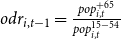 $odr_{i,t-1} = \frac {pop^{+65}_{i,t}}{pop^{15-54}_{i,t}}$
and lagged unemployment ratio to working-age population
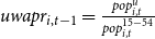 $uwapr_{i,t-1} = \frac {pop^{u}_{i,t}}{pop^{15-54}_{i,t}}$
, enter through parameters
 $\mu _{i1}, \mu _{i2}$
that we will test whether they are common to all countries (i.e.
 $\mu _{i1}=\mu _1$
for all
 $i$
and
 $\mu _{i2}=\mu _2$
for all
 $i$
). Two additional (possibly country-specific) drivers, the growth rate of the old-age dependency ratio
 $odrg_{i,t}$
and the change in the unemployment ratio
 $\Delta uwapr_{i,t}$
, are captured by
 $\mu _{3,i}$
and
 $\mu _{4,i}$
respectively.
The general state-space model (measurement equation (20) plus transition equation) is estimated by (quasi) maximum likelihood using the Kalman filter. In the empirical results section, we consider restricted variants (e.g., common vs. country-specific
 $\phi _i$
; exclusion of demographic drivers) nested within this general specification.
The estimated (inverse) tax-tilting parameter
 $\theta ^{-1}_{i,t}$
is related to structural discount factors through:
 \begin{equation*} \theta = \frac {1 - \frac {\Psi }{\beta }\cdot \Psi }{1 - \Psi }, \qquad \Psi = \frac {1+\nu }{1+i} = \frac {1}{1+\psi }, \end{equation*}
where
 $\Psi$
is the (observed) market discount factor implied by nominal GDP growth
 $\nu$
and the nominal interest rate
 $i$
(with
 $\psi$
the growth-adjusted interest rate). Given an estimate of
 $\theta$
and observed
 $\Psi$
, the implied subjective discount factor
 $\beta$
is recovered as:
 \begin{equation} \beta = \frac {\Psi ^{2}}{1 - \theta \cdot (1 - \Psi )} = \frac {\Psi ^{2}}{1 - \theta + \theta \cdot \Psi }, \end{equation}
which corresponds to a subjective discount rate
 $\delta$
defined by:
 \begin{equation} \beta = \frac {1}{1+\delta }. \end{equation}
This mapping permits the interpretation of estimated tilting behavior in terms of underlying intertemporal preferences.
4. Data and time-series properties analysis
This section documents the data, sources, procedures used to construct the variables, and the univariate time-series properties of the fiscal and demographic variables employed in the empirical analysis. We begin by performing unit root tests for the fiscal variables: primary (non-interest) government expenditure (
 $g_t$
), nominal interest service on lagged debt (
 $i_t b_{t-1}$
), total government expenditure (
 $g^{tot}_t$
), and tax revenue (
 $\tau _t$
), all expressed as ratios to GDP. After establishing the order of integration of these series, we proceed (in subsequent sections) to estimate a potential cointegration relationship and the associated time-varying tilting parameter for a panel of EMU countries, paying particular attention to its evolution and possible convergence patterns relevant for deepening fiscal integration.
4.1 The data
Fiscal data were extracted from the European Commission AMECO (Annual Macro-Economic) database for the period 1970–2024. The sample comprises a group of “peripheral” EMU economies (Portugal, Ireland, Italy, Greece, Spain, and Finland) together with core Euro Area members (Germany, France, Belgium, the Netherlands, and Austria). Eastern Euro Area economies are excluded due to shorter and less homogeneous data availability.
Constructing homogeneous long-run fiscal series requires addressing two main sources of discontinuity: (i) changes in the European System of Accounts (ESA79 for roughly 1970–1995, ESA95 for 1995–2010, and ESA 2010 thereafter) and (ii) the German reunification break. Following Paredes et al. (Reference Paredes, Pedregal and Pérez2009), we eliminate level discontinuities by iteratively “back-casting” earlier vintages using growth rates from the subsequent accounting standard. Specifically, to obtain a consistent ESA95* level compatible with ESA2010, and analogously for earlier breaks, we apply:
 \begin{equation} Y_{t-1}^{\text{ESA95}^*} = \dfrac {Y_{t}^{\text{ESA95}}}{\left (\frac {Y_{t}^{\text{ESA79}}}{Y_{t-1}^{\text{ESA79}}}\right )}. \end{equation}
This recursive adjustment is applied successively so that historical segments are expressed on a common latest-standard methodological basis.
The panel thus constructed possesses both adequate time depth and cross-sectional variation to support robust estimation of the time-varying specification.
The effective government interest rate is computed directly as the ratio of net interest payments during fiscal year
 $t$
to the average stock of government debt held by the public over that year. Because this is a simple (period) rate, we convert it to an equivalent compound annual rate for consistency. Whenever expressions such as
 $i_t - \nu _t$
appear,
 $i_t$
denotes this compound interest rate and
 $\nu _t$
nominal GDP growth.
In line with Cho and Lee (Reference Cho and Lee2022), we use the old-age dependency ratio,
 $odr_{i,t}$
, as a demographic indicator, defined as the population aged 65 and over divided by the working-age population (15–64). This ratio is constructed from AMECO demographic series.
Additionally, from the OECD database we retrieve a set of variables related to the fiscal impact of aging: (i) the social security contributions ratio to GDP,
 $ssc_{i,t}$
; (ii) total social security expenditure,
 $ss^{tot}_{i,t}$
; and (iii) public pension expenditure,
 $ss^{pen}_{i,t}$
; all expressed as shares of GDP. The social expenditure series are available from 1980 onward.
4.2 Univariate properties of the data
We next analyze the order of integration of the fiscal variables (all as GDP ratios), allowing for the presence of structural breaks and cross-sectional dependence. As emphasized by Perron (Reference Perron1989), failing to model structural breaks can lead to spurious evidence of unit roots.Footnote 3 Distinguishing between stochastic and deterministic sources of non-stationarity carries substantive policy implications: if trends are stochastic, shocks have permanent fiscal effects with potential solvency risks; if breaks are deterministic (level or trend shifts), deviations may be transitory and correctable through policy interventions (Nguyen et al. Reference Nguyen, Suardi and Chua2017).
To accommodate multiple structural breaks and cross-section dependence, we employ the panel unit root procedures of Bai and Carrion-i Silvestre (Reference Bai and Carrion-i Silvestre2009), which pool modified Sargan-Bhargava statistics (Sargan and Bhargava, Reference Sargan and Bhargava1983). Their framework allows for (i) multiple break dates in each series, where break detection adapts the methodology of Bai and Perron (Reference Bai and Perron2003) to the panel context. and (ii) a general common factor structure capturing cross-section dependence, following Bai and Ng (Reference Bai and Ng2004) and Moon and Perron (Reference Moon and Perron2004). Common factors may themselves be stationary, non-stationary, or a mixture. The number of factors is selected using the panel Bayesian Information Criterion of Bai and Ng (Reference Bai and Ng2002).
In implementation, we allow up to four structural breaks per series, with break dates selected via the Bai and Perron (Reference Bai and Perron1998) procedure.Footnote 4 Applied to our 11-country panel, the tests yield strong evidence of multiple structural breaks across most fiscal variables, with substantial heterogeneity in both number and timing.
After controlling for common factors and allowing for structural breaks, the null of a unit root cannot be rejected for these variables across both the “conventional” and “simplified” test variants.Footnote 5
The joint presence of (i) non-rejection of unit roots in the core fiscal ratios and (ii) multiple breaks of heterogeneous timing across countries is consistent with the existence of a cointegrating relationship among revenue, expenditure, and interest service variables. This finding motivates the subsequent estimation of a (possibly time-varying) long-run fiscal equilibrium vector and the extraction of the tax-tilting parameter dynamics reported later in the paper.
5. Results and discussion
5.1 State-space model estimation
This subsection reports the estimation of the empirical state-space specification introduced in Section 3. As shown in Hamilton (Reference Hamilton, Engle and McFadden1994), among others, state-space methods provide a flexible framework for modeling TVPs. We implement our estimation using sspaneltvp, a GAUSS toolbox developed by Camarero et al. (Reference Camarero, Sapena and Tamarit2025) to estimate fully-fledged panel time-varying parameter (TVP) models via the Kalman filter.
The sspaneltvp environment extends the univariate setup in Hamilton (Reference Hamilton, Engle and McFadden1994) to a panel context with both fixed (common or country-specific) and stochastic time-varying components. Under suitable parameter restrictions, the system nests mean-reverting specifications, and the fixed (mean) component may include a deterministic trend. The transition equation admits autoregressive alternatives and exogenous “drivers” (control instruments) whose coefficients can be imposed as common across countries or allowed to vary idiosyncratically for uncovering asymmetric responses to common shocks. In addition, the GAUSS code supports user-defined restrictions on the variance-covariance matrices of both the transition and measurement equations.Footnote 6
To select our baseline model, we compare a general unrestricted model with alternative specifications nested within the general state-space model presented in Section 3 and equations (20) and (24). We compare the unrestricted model with several alternative specifications, where we reduce the heterogeneity of the different parameters in the two equations.
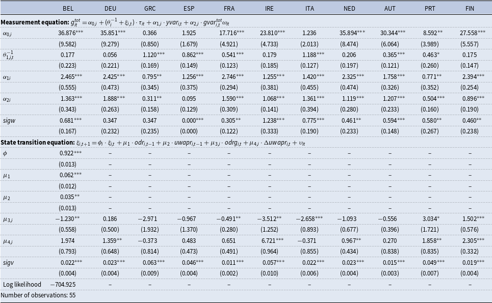
State-space tax tilting 1970-2024. Selected EMU countries

Table 1. Long description
A table comparing state-space tax tilting for selected EMU countries from 1970 to 2024. The table has 12 columns and 11 rows, including headers and notes. Columns are labeled with country codes: BEL, DEU, GRC, ESP, FRA, IRE, ITA, NED, AUT, PRT, FIN. Row labels include measurement equation parameters (α0j, θ⁻¹, α1, α2, sigw) and state transition equation parameters (φ, μ1, μ2, μ3j, μ4j, sigv). Each cell contains numerical values with standard deviations in parentheses. Notable trends include significant values marked with asterisks indicating levels of statistical significance. The table also includes log likelihood and number of observations at the bottom.
Notes: standard deviations in parentheses. *
 $p\lt 0.10$
, **
 $p\lt 0.05$
, ***
 $p\lt 0.01$
.
The choice of the model specification has been made using a sequential procedure relying on likelihood ratio tests, which led to the preferred specification (Model 3), where two control inputs in the transition equation (
 $odr$
and
 $uwapr$
) entered with common parameters.Footnote
7
The results of the implemented tests favor the chosen specification against these alternatives. In particular, they support idiosyncratic tax-tilting behavior among countries; the relevance of considering demographic factors and unemployment dynamics, as well as a highly persistent autoregressive parameter against a random walk.
The maximum-likelihood estimates of the hyperparameter vector are reported in Table 1. The fixed component of the (inverse) tax-tilting parameter,
 $\bar {\theta }^{-1}_i$
, is statistically significant for Greece, Spain, France, Italy, Austria and Portugal. Point estimates cluster into two broad groups. For core EMU countries, the effect is only significant in the case of Austria and France, with values
 $\bar {\theta }^{-1}=0.365$
and
 $0.541$
, respectively. Portugal could also be included in this group, as its parameter is around
 $0.5$
. This implies tilting toward the present (i.e., proportionally more current taxation). In Greece and Italy, we obtain
 $\bar {\theta }^{-1}_i \gt 1$
, consistent with tilting toward the future and thus with a structural tendency to run current budget deficits as a share of GDP. Finally, in Spain, the parameter is large but below one (
 $0.862$
).
Turning to the lower half of the table and state (transition) dynamics of
 $\theta ^{-1}_{i,t}$
, the panel-common coefficients on the lagged old-age dependency ratio (
 $\mu _1$
) and the unemployment-to-working-age-population ratio (
 $\mu _2$
) are both positive and statistically significant. This suggests that demographic aging and labor market slack each contribute to widening the gap between government expenditure needs and contemporaneous taxation, interpretable as a decrease in
 $\theta _i$
and therefore increased tax tilting toward the future. It is important to note that, although exhibiting a common parameter, worsening conditions in the labor market are especially harmful for countries exhibiting higher unemployment, as is the case of peripheral countries, specifically Spain.
As for the second group of parameters, which are
 $\mu _{3i}$
and
 $\mu _{4i}$
, the country-specific responses to the growth of these demographic and labor market variables, several patterns emerge. First, some countries react strongly to aging pressures and others to changes in unemployment. Second, for most countries with a significant
 $\mu _3$
coefficient, the response to growth in old-dependency is negative (Belgium, France, Ireland and Italy), but for Portugal and Finland it is positive. Third,
 $\mu _4$
is only positive and significant for Germany, Ireland, the Netherlands, Portugal and Finland.
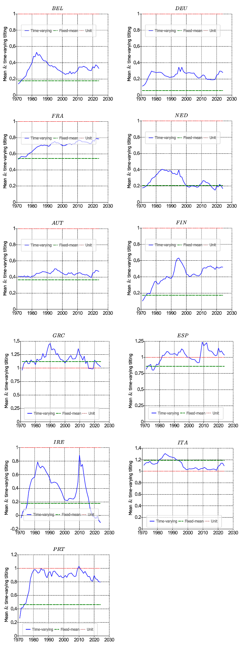
Time-varying tax-tilting parameters. Core EMU countries.

Figure 1 plots the estimated time-varying deviations of the country-specific coefficient around its mean implied by the mean-reverting transition equation. Core countries have a fixed-mean (green line) around
 $0.4$
or below (Belgium, Germany, the Netherlands, Austria, and Ireland). France’s mean is close to
 $0.6$
, but the trend of the time-varying parameter is worsening in the latter. Italy’s mean is around
 $1.2$
and Greece’s is close to
 $1.2$
, but the trend of its time-varying parameter is decreasing in both. In the case of Spain, the fixed-mean is below 1 but has deteriorated steadily since the 1980s, when it crossed the value 1. After 2000, its value returned below 1, only to worsen again with the financial crisis. Portugal’s mean is around
 $0.5$
, but the time-varying parameter has approached 1 since 1980. Following the financial crisis and subsequent bailout, the rate has been decreasing.
5.2 Tilting, taxes and subjective time preferences
Given the estimated mean values of the tilting parameter
 $\theta _i$
and the observed values of the market discount factor
 $\Psi _i$
, we can recover the implied subjective discount factor
 $\beta _i$
for each country using the following relationship. Starting from the expression:
 \begin{equation} \theta = \frac {1 - \frac {\Psi }{\beta } \cdot \Psi }{1 - \Psi }, \end{equation}
we solve for
 $\beta$
to obtain:
 \begin{equation} \beta = \frac {\Psi ^2}{1 - \theta \cdot (1 - \Psi )} = \frac {\Psi ^2}{1 - \theta + \theta \cdot \Psi }. \end{equation}
This formula links the government’s subjective discount factor
 $\beta$
to the estimated tilting parameter
 $\theta$
—which governs the intertemporal trade-off between taxes and expenditure—and the effective market discount factor
 $\Psi$
, which incorporates observed interest and growth rates.
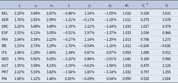
To illustrate, Table 2 presents country-level results for the year 2024. Based on the values in the first five columns (from
 $i_t$
to
 $\gamma _i$
), we compute the growth-adjusted interest rate
 $\psi _i$
and the corresponding discount factor
 $\Psi _i$
. These, together with country-specific estimates of the inverse tilting parameter
 $\theta ^{-1}$
, allow us to derive both
 $\theta$
and the implied
 $\beta$
for each country.
2024 values for interest rate, GDP growth, effective interest rate,
 $\Psi$
and
 $\theta$

Table 2. Long description
A table comparing economic indicators for various countries in 2024. The table has 12 rows and 10 columns. The columns are labeled as follows: i_j, v_j, π_j, r_j, γ_j, ψ_j, Ψ_j, σ_j^(-1), and θ_j. The rows are labeled with country codes: BEL, GER, GRC, ESP, FRA, IRE, ITA, NED, AUT, PRT, and FIN. Each row presents values for interest rate, GDP growth, effective interest rate, and other economic indicators for the respective country. For example, BEL has an interest rate of 2.20 percent, GDP growth of 3.84 percent, and an effective interest rate of 2.67 percent. The table provides a detailed comparison of these economic indicators across different countries.
Interestingly, in 2024, only Italy and Finland exhibit positive effective market rates (
 $\Psi \lt 1$
). Moreover, negative effective market rates are particularly favorable for peripheral countries, specifically Spain, Portugal, and Greece. Given their specific subjective discount factors, the market stance would be incentivizing their tilting behavior.
The tilting parameter
 $\theta$
captures the deviation from the benchmark of perfect tax smoothing. When
 $\theta = 1$
, the government discounts the future at the same rate as the market, implying neutral intertemporal preferences and a flat tax path over time. If
 $\theta \gt 1$
, the government is relatively more impatient than the market (i.e.,
 $\beta \lt \Psi$
): it places greater weight on present fiscal costs, leading to more front-loaded taxation and quicker adjustment. Conversely, when
 $\theta \lt 1$
, the government is more patient than the market (i.e.,
 $\beta \gt \Psi$
), leading to a preference for delayed fiscal effort and greater reliance on future adjustments. These differences affect not only the timing of fiscal consolidation but also the intertemporal allocation of welfare and potential trade-offs between short-run economic stability and long-run sustainability.
We observe that for Greece, Spain, Italy, and Portugal, the estimated tilting parameter lies below unity (
 $\theta \lt 1$
), indicating a preference for delaying tax adjustments relative to the tax-smoothing benchmark. This suggests a higher effective government discount factor compared to the market (
 $\beta \gt \Psi$
), consistent with a more patient intertemporal fiscal stance. In contrast, although both Italy and Finland display market discount factors
 $\Psi$
below one—indicating that real interest rates exceed output growth—their resulting tilting parameters diverge: in Italy,
 $\theta \lt 1$
, reinforcing the tendency to back-load fiscal effort, whereas in Finland,
 $\theta \gt 1$
, reflecting a more front-loaded approach and closer alignment with tax-smoothing principles.
To further interpret the implied government discount factor
 $\beta$
, we decompose it to isolate the contributions of pure time preference and expected consumption growth. Adapting the Ramsey framework, we express the relationship as:
 \begin{equation} \frac {1}{1+\rho } = \frac {1 + E[\eta ]^\alpha }{1 + \delta }, \end{equation}
which implies:
 \begin{equation} \frac {1}{1+\rho } = \beta \cdot (1 + E[\eta ]^\alpha ). \end{equation}
This formulation links the pure rate of time preference
 $\rho$
to the subjective discount factor
 $\beta$
and the expected growth rate of consumption
 $E[\eta ]$
, raised to the elasticity of marginal utility
 $\alpha$
.
To implement this expression empirically, we adopt two standard assumptions applied uniformly across countries. First, we approximate
 $E[\eta ]^\alpha$
using the geometric mean of real GDP growth, denoted
 $\gamma$
, over the sample period. Second, we set
 $\alpha = 1$
, corresponding to logarithmic utility—a conventional assumption in intertemporal macroeconomic modeling.Footnote
8
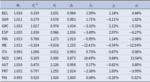
Values in 2024 of tilting, subjective discount factors and idiosyncratic rate of pure time preference,
 $\rho$

Table 3. Long description
Panel A: Line graph showing the relationship between tilting and subjective discount factors. The x-axis represents subjective discount factors with units in percent, and the y-axis represents tilting with units in percent. The graph shows a positive trend where tilting increases with higher subjective discount factors. Panel B: Line graph showing the relationship between tilting and idiosyncratic rate of pure time preference. The x-axis represents idiosyncratic rate of pure time preference with units in percent, and the y-axis represents tilting with units in percent. The graph shows a positive trend where tilting increases with higher idiosyncratic rate of pure time preference.
Table 3 reports, for 2024, the estimated pure rates of time preference
 $\rho _i$
, obtained by adjusting the subjective discount factors
 $\beta _i$
for expected real GDP growth (
 $\gamma _i$
) in line with the Ramsey framework. The results reveal marked cross-country heterogeneity in intertemporal fiscal preferences.
In Belgium, Italy, Austria, and Finland,
 $\rho _i$
is close to zero (between
 $0.06\%$
and
 $0.80\%$
), indicating broadly neutral intertemporal preferences once growth expectations are incorporated. Governments in these countries neither strongly front-load nor postpone taxation relative to the tax-smoothing benchmark. Germany exhibits a moderately positive
 $\rho$
(
 $1.82\%$
), suggesting a slight preference for present fiscal benefits, whereas the Netherlands stands out with a very high
 $\rho$
(
 $13.54\%$
), consistent with a pronounced front-loading bias. Such elevated values may partly reflect optimistic long-run growth or productivity assumptions, given that the decomposition corrects
 $\beta$
using
 $\gamma _i$
.
By contrast, several economies show negative
 $\rho _i$
values, indicating greater patience than implied by market interest rates. The most extreme cases are Ireland (
 $-12.94\%$
) and the southern EMU countries—Greece, Spain, and Portugal—with
 $\rho _i$
between
 $-3.95\%$
and
 $-6.27\%$
. In these cases, governments place relatively more weight on the future than the market does, which—combined with low or negative effective interest rates—creates incentives to postpone tax increases. France also registers a moderately negative
 $\rho$
(
 $-2.06\%$
), pointing in the same direction.
The magnitude of
 $\theta$
in these countries reinforces this interpretation. For Greece and Spain,
 $\theta \lt 1$
but close to unity, signaling a systematic delay in fiscal adjustment. In Portugal, by contrast,
 $\theta \gt 1$
despite a negative
 $\rho$
, suggesting that other constraints or policy choices may drive a modest front-loading tendency. The extreme negative
 $\rho$
in Ireland corresponds to a negative
 $\theta$
, which in practice signals a breakdown of the simple tilting logic—likely reflecting exceptional macroeconomic factors, such as volatile GDP data driven by multinational activity.
An interesting finding of the research is the different patterns observed when facing a negative effective interest rate on public debt (e.g.,
 $-2\%$
). For some governments, the estimated value of
 $\theta ^{-1}\gt 1$
(or
 $\theta \lt 1$
) implies a government’s subjective discount rate, which is also negative but higher (e.g.,
 $-2.5\%$
). This implies that the government places more value on future outcomes than the market does and optimally chooses to postpone tax increases heavily. Expectations of stronger future fiscal capacity can justify such behavior, the desire to smooth tax distortions during periods of high current costs, or the low cost of debt rollover in a negative-rate environment. It may also reflect features of secular stagnation or dynamic inefficiency, where delaying taxes improves welfare. However, while such stances may be optimal in the short run, their persistence raises questions about the credibility and sustainability of long-term fiscal adjustment—particularly if underlying assumptions about growth or interest rates prove overly optimistic.
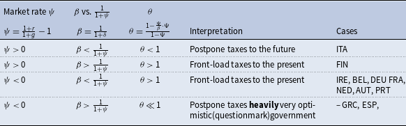
Table 4 summarizes the combinations of market discount rates (
 $\psi$
), government subjective discount factors (
 $\beta$
), and the resulting tilting parameters (
 $\theta$
), along with the associated fiscal behavior across EMU countries.
Values of
 $\psi$
and
 $\beta$
and implied values of
 $\beta$
for
 $\theta$

Table 4. Long description
A table comparing market discount rates, government subjective discount factors, and tilting parameters across EMU countries. The table has 15 rows and 7 columns. Column headers are Ψj, θj^-1, θj, βj, δj, ηj, and ρj. Row labels are BEL, GER, GRC, ESP, FRA, IRE, ITA, NED, AUT, PRT, and FIN. Row 1: BEL, 1.016, 0.330, 3.031, 0.984, 1.59, 1.14, 0.44. Row 2: GER, 1.011, 0.279, 3.578, 0.983, 1.71, -0.11, 1.82. Row 3: GRC, 1.033, 1.027, 0.974, 1.034, -3.32, 2.12, -5.33. Row 4: ESP, 1.035, 1.036, 0.966, 1.036, -3.49, 2.97, -6.27. Row 5: FRA, 1.013, 0.786, 1.273, 1.010, -0.95, 1.14, -2.06. Row 6: IRE, 1.012, -0.104, -9.636, 1.155, -13.41, -0.54, -12.94. Row 7: ITA, 0.993, 1.096, 0.912, 0.993, 0.73, 0.67, 0.06. Row 8: NED, 1.041, 0.169, 5.900, 0.873, 14.49, 0.84, 13.54. Row 9: AUT, 1.016, 0.470, 2.126, 0.998, 0.17, -0.62, 0.80. Row 10: PRT, 1.032, 0.797, 1.255, 1.024, -2.36, 1.65, -3.95. Row 11: FIN, 0.995, 0.520, 1.924, 1.000, 0.04, -0.28, 0.32.
Italy is the only country in the sample where both the market rate
 $\psi$
is positive and the implied government discount factor
 $\beta$
is relatively low, leading to a tilting parameter
 $\theta \lt 1$
. This configuration suggests a preference for deferring tax increases to the future, which may reflect either expectations of future fiscal capacity or an attempt to smooth tax distortions over time under persistently high debt ratios.
Finland, by contrast, also exhibits a positive
 $\psi$
but with a high value of
 $\beta$
, implying
 $\theta \gt 1$
. This corresponds to front-loading of taxes, consistent with a more conservative fiscal stance and a stronger emphasis on intertemporal budgetary discipline. In this case, the government places relatively more weight on current consolidation efforts than on future adjustments.
The majority of the sample—including Ireland, Belgium, Germany, France, the Netherlands, Portugal and Austria—falls into the third category, where
 $\psi \lt 0$
and
 $\beta \lt \frac {1}{1+\psi }$
, resulting in
 $\theta \gt 1$
. Despite the presence of negative growth-adjusted interest rates, these governments exhibit a relatively impatient stance, opting to front-load taxes. This behavior may reflect concerns about fiscal sustainability, institutional constraints, or a conservative interpretation of the no-Ponzi condition, even under favorable borrowing conditions.
The final group consists of Greece and Spain, which combine negative
 $\psi$
with relatively high
 $\beta$
, yielding values of
 $\theta \ll 1$
. These countries exhibit strong tax tilting toward the future, consistent with either optimistic expectations about future fiscal conditions or strategic delay in adjustment facilitated by negative effective interest rates. This behavior results in an intertemporal profile where present taxation is low relative to future requirements, raising concerns about the long-term credibility of fiscal consolidation paths—especially in the event of a reversal in interest rate conditions or growth prospects.
Overall, the dispersion in
 $\theta$
across countries reflects meaningful differences in fiscal preferences and constraints. While some of the heterogeneity can be explained by differences in borrowing costs and growth expectations, the resulting fiscal paths highlight the challenges of achieving coordination and convergence in a monetary union with decentralized fiscal policies.
To complement the cross-sectional evidence, Figure 2 depicts the time-varying evolution of the key parameters
 $\beta _{i,t}$
and
 $\psi _{i,t}$
for some countries in our sample.Footnote
9
The upper row corresponds to core EMU economies, while the lower panel focuses on the peripheral group. In the latter, both series almost coincide for most of the sample, suggesting that governments’ intertemporal discounting behavior is closely aligned with prevailing financial market conditions. This alignment points to a fiscal stance largely shaped by market constraints and incentives, potentially leaving limited room for autonomous, forward-looking policy decisions—an indication of possible political bias in tax-smoothing behavior. By contrast, core economies display a more stable trajectory for
 $\beta _{i,t}$
, less sensitive to short-term fluctuations in
 $\psi _{i,t}$
. Sometimes, they even display a mirroring behavior. These countries tend to leverage favorable market conditions not to increase indebtedness, but to accelerate debt repayment and strengthen fiscal positions, consistent with a more proactive and countercyclical approach to debt management.
Time-varying tax-tilting parameters and effective interest rates. Core EMU countries.

Overall, reducing the social, political, and demographic sources of heterogeneity documented here would facilitate debt mutualization and strengthen the institutional foundations for a future fiscal union in the Euro Area.
6. Conclusions
This paper employs a panel Time-Varying Parameter (TVP) state-space framework to estimate tax-tilting behavior across 11 EMU member states. Our findings reveal substantial heterogeneity in intertemporal fiscal behavior, allowing countries to be grouped into two broad categories.
Several core EMU members, such as Austria, Belgium, Germany, the Netherlands, France, Ireland, and Finland, exhibit a relatively prudent fiscal stance, with tax tilting that supports intertemporal budget discipline. In contrast, peripheral countries, namely Greece, Italy, Portugal, and Spain, tend to tilt taxation toward the future
 $(\theta _{i,t}^{-1} \gt 1)$
, thereby incurring present fiscal deficits. This behavior reflects a preference for financing current expenditures by deferring tax efforts to future periods.
A central insight of our analysis is that such tax-tilting patterns are driven by a divergence between the government’s subjective discount factor and the effective market discount factor used to value future tax revenues. Using a Ramsey framework, we estimate country-specific rates of pure time preference that shed light on the intertemporal decision-making behind observed fiscal trajectories.
We also identify important asymmetries in the impact of structural variables. The old-age dependency ratio, in particular, tends to exacerbate fiscal tilting in some countries, suggesting that demographic pressure undermines efforts to maintain intertemporal balance. Similarly, higher unemployment relative to the working-age population is associated with more pronounced deferral of tax obligations.
A critical macroeconomic context is the presence of persistently negative effective real interest rates
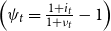 $\left (\psi _t = \frac {1+i_t}{1+\nu _t} - 1\right )$
, or equivalently an effective market factor
 $\left (\Psi _t = \frac {1}{1+\psi _t}\right )$
greater than one. In such a setting, the intertemporal government budget constraint (GIBC) relaxes, as the real value of public debt declines over time. This dynamic may allow governments to roll over debt and generate a net fiscal surplus without raising taxes, effectively acting as a “negative” tax burden.
Under these conditions, some governments appear to operate with a subjective discount factor
 $\beta \gt 1$
, exceeding both unity and the market factor. This leads them to “anticipate this negative tax burden to the present”, expanding current expenditure and worsening present deficits. When the “required taxes to meet the GIBC are negative”, such behavior can be interpreted as the intertemporal valuation of future fiscal payoffs in a context where the marginal cost of postponing taxation is also negative.
These findings raise important considerations regarding long-term fiscal sustainability and the credibility of future policy adjustments. More broadly, they suggest that addressing the deep-rooted heterogeneities (be they social, political, or demographic) is essential for facilitating debt mutualization and advancing toward a more integrated fiscal union within the Euro Area. Convergence in fiscal behavior and preferences appears to be a necessary precondition for deeper economic integration among EMU member states.
Our findings also speak directly to the ongoing reform of European fiscal governance. The EU’s new Economic Governance Framework, formally adopted in April 2024 (Regulation (EU) 2024/1263 and Directive (EU) 2024/1264), replaced the Stability and Growth Pact’s uniform numerical targets with country-specific medium-term fiscal-structural plans, explicitly acknowledging the heterogeneity in fiscal starting positions and adjustment capacities across member states (European Commission, 2024). Our results provide empirical grounding for this institutional shift: the substantial and persistent cross-country dispersion in estimated tilting parameters
 $\theta _{i,t}$
—rooted in divergent demographics, labor-market conditions, and subjective discount rates—implies that one-size-fits-all deficit or expenditure ceilings are poorly suited to achieving intertemporal fiscal equity across the union. At the same time, the persistence of future-biased taxation in peripheral economies raises legitimate concerns about whether country-specific plans, absent stronger supranational enforcement or coordination mechanisms, will suffice to ensure long-run debt sustainability. These considerations reinforce proposals for a genuine central fiscal capacity at the euro-area level—one capable both of absorbing asymmetric shocks and of providing credible intertemporal commitment in member states where the incentive to delay taxation is strongest (Carnot et al. Reference Carnot, Kizior and Mourre2017; Dolls et al. Reference Dolls, Fuest, Heinemann and Peichl2016). Our time-varying estimates of
 $\theta _{i,t}$
could, in principle, help calibrate such a capacity by identifying the countries and time periods in which the divergence between private and social intertemporal discounting is largest, and where cross-border risk sharing would therefore deliver the greatest welfare gains.
Supplementary material
The supplementary material for this article can be found at https://doi.org/10.1017/S1365100526101412.
Acknowledgements
The authors are indebted to J.D. Hamilton and J.LL. Carrion-i-Silvestre for providing their Gauss codes, and also to Eric Clower, from Aptech Systems, for the technical advice and refinement of some parts of the code. They also thank A. Torój and the participants in the 9th Internat. Workshop on Financ. Markets & Nonlinear Dynamics (Paris), and the 27th INFER Annual Conference (Rome) for their comments and suggestions. The authors acknowledge the public funding from MCIU/AEI (Project PID2023-150095NB-C42/10.13039/501100011033) and the Valencian regional government (Generalitat Valenciana-PROMETEO CIPROM/2022/50 project). J. Sapena is also grateful to the Chair “Christeyns” for a Sustainable Economic Development for its specific funding of this research. C. Tamarit acknowledges funding from the European Commission project GEaR-EU - 101234793. The European Commission’s support does not constitute an endorsement of the contents, which reflect the views only of the authors, and the Commission cannot be held responsible for any use that may be made of the information contained therein.
Competing interests
On behalf of all authors, the corresponding author states that there is no conflict of interest. All remaining errors are ours.


 Ψ
 θ
 ρ
 ψ
 β
 β
 θ



