1 Introduction
Hydraulic fracturing is a well-established technique to stimulate oil and gas wells (Economides & Nolte Reference Economides and Nolte2000), and it also occurs in nature in the form of magma dikes (Spence & Turcotte Reference Spence and Turcotte1985; Lister Reference Lister1990) and fluid-filled glacial cracks (Tsai & Rice Reference Tsai and Rice2010). Fluid flow inside a fracture is a key component that is required for modelling of a hydraulic fracturing process. Most models use a laminar flow solution since fluids with large viscosities, such as gels, are often used for stimulation of oil and gas wells. Large values of the magma viscosity naturally lead to the use of a laminar flow solution as well. Glacial cracks, on the other hand, are filled with water. Moreover, with the development of hydraulic fracturing, low-viscosity water-based fluids are frequently used. With the reduction of viscosity by several orders of magnitude, the assumption of laminar flow may not always be valid, in which case turbulent flow models should be employed.
Several studies have used turbulent fluid flow models for hydraulic fracturing. In early works (Nilson Reference Nilson1981; Emerman, Turcotte & Spence Reference Emerman, Turcotte and Spence1986), the turbulent flow model was applied to plane strain fractures. Later, the same model was utilized by Anthonyrajah, Mason & Fareo (Reference Anthonyrajah, Mason and Fareo2013) to study the propagation of fractures with the Perkins–Kern–Nordgren (PKN) geometry. A different turbulent flow model was used by Tsai & Rice (Reference Tsai and Rice2010) to analyse the propagation of plane strain cracks in glaciers. The latter model was then applied to PKN fractures by Ames & Bunger (Reference Ames and Bunger2015), targeting petroleum applications. In contrast to the aforementioned studies, where turbulent flow of a Newtonian fluid was considered, a turbulent model for a power-law fluid is described in Kresse & Weng (Reference Kresse, Weng, Bunger, McLennan and Jeffrey2013). Most of these models (except, e.g., Nilson Reference Nilson1981) share the same weakness, which is an inability to simultaneously describe both laminar and turbulent flow within the same fracture. Since the Reynolds number is proportional to the fracture width, which vanishes at the fracture tip, there is always a laminar flow in the near-tip region. To account for both the laminar and turbulent regimes, one possibility is to switch from a laminar to a turbulent model based on the Reynolds number. This study employs a different approach, in which a universal fluid flow model that captures the laminar, turbulent and transition regimes is utilized. To better understand the effects associated with turbulent flow, a semi-infinite hydraulic fracture is analysed. Such a problem describes the near-tip behaviour of a hydraulic fracture, and enables one to observe the transition between fracture shapes associated with laminar and turbulent flows.
2 Turbulent flow in pipes
Flow in pipes has been studied extensively during the last century, see, e.g., Benedict (Reference Benedict1980). In many practical applications, the pressure drop in a pipe is calculated based on the phenomenological Darcy–Weisbach equation,
 $$\begin{eqnarray}\displaystyle -\frac{\partial p}{\partial x}=f_{D}\frac{{\it\rho}}{2}\frac{U^{2}}{D}, & & \displaystyle\end{eqnarray}$$
where
 $U$
is the mean velocity in the pipe,
 $D$
is the diameter,
 ${\it\rho}$
is the fluid mass density,
 $\partial p/\partial x$
is the pressure gradient along the pipe and
 $f_{D}$
is the dimensionless friction factor. The aforementioned friction factor has been measured experimentally, and the observations are summarized on the so-called Moody chart (Moody Reference Moody1944), which provides the values of
 $f_{D}(Re,{\it\epsilon})$
for different Reynolds numbers and wall roughnesses. Here, the Reynolds number is defined as
 $Re={\it\rho}UD/{\it\mu}$
, where
 ${\it\mu}$
is the fluid viscosity, while the wall roughness,
 ${\it\epsilon}$
, has a dimension of length. There are numerous empirical formulae for the friction factor, which are used for the calculations. Most of them, however, focus exclusively on the turbulent regime, and are not able to capture laminar flow, e.g. Benedict (Reference Benedict1980). One exception is the empirical approximation proposed by Churchill (Reference Churchill1977), which approximates the whole Moody chart, and provides values of
 $f_{D}$
for the laminar (
 $Re<2000$
), turbulent (
 $Re>3000$
) and transition regimes (
 $2000<Re<3000$
). The formula for the friction factor can be written as
 $$\begin{eqnarray}\displaystyle f_{D}=8\left(\left(\frac{8}{Re}\right)^{12}+(A+B)^{-1.5}\right)^{1/12}, & & \displaystyle\end{eqnarray}$$
where the parameters
 $A$
and
 $B$
are given by
 $$\begin{eqnarray}\displaystyle A=\left(2.457f_{0}\left(Re,\frac{{\it\epsilon}}{D}\right)\right)^{16},\quad B=\left(\frac{37530}{Re}\right)^{16},\quad f_{0}(Re,r)=\left|\log \!\left(\!\left(\frac{7}{Re}\right)^{0.9}\!+0.27r\right)\right|. & & \displaystyle \nonumber\\ \displaystyle & & \displaystyle\end{eqnarray}$$
It should be noted that the maximum value of roughness shown on the Moody chart is typically
 ${\it\epsilon}/D=0.05$
. In this case, the validity of (2.2) beyond
 ${\it\epsilon}/D=0.05$
is not justified. Indeed, in situations when the roughness parameter increases to
 $O(1)$
, the flow becomes qualitatively different due to the tortuosity effect. The modification of (2.2) to account for large values of the roughness requires an additional investigation and is beyond the scope of this study.
3 Turbulent flow in fractures
Flow in fractures is equivalent to flow between two parallel plates, and therefore is different from the flow in circular pipes. Turbulent flow in pipes with non-circular cross-sections is often described through a concept of hydraulic diameter, since the turbulent friction factor is only weakly dependent upon the duct shape (Benedict Reference Benedict1980). Here, the hydraulic diameter is defined as
 $D_{h}=4A/P$
, where
 $A$
is the cross-sectional area while
 $P$
is the perimeter of the channel. The hydraulic diameter is equal to the actual diameter for circular pipes, but for the flow in a fracture of width
 $w$
the hydraulic diameter is
 $D_{h}=2w$
.
The friction coefficient for the laminar regime, however, strongly depends on the shape of the duct, and for a fracture is
 $f_{D}=96/Re$
, which upon substitution in (2.1) reduces to the well-known relation
 $U=-w^{2}/(12{\it\mu})\partial p/\partial x$
. On the other hand, the friction factor for circular pipes for the laminar regime is
 $f_{D}=64/Re$
, as can also be seen from (2.2).
Since the first term in (2.2) dominates in the laminar regime, while the parameters
 $A$
and
 $B$
are responsible for the turbulent regime, one possibility to adapt the empirical formula for pipes to capture flow in fractures is to change the ‘laminar’ term so that it captures the laminar solution, in which case (2.2) becomes
 $$\begin{eqnarray}\displaystyle f_{D}=8\left(\left(\frac{12}{Re}\right)^{12}+(A+B)^{-1.5}\right)^{1/12}. & & \displaystyle\end{eqnarray}$$
It should be noted that the Reynolds number utilizes the concept of hydraulic diameter, i.e.
 $D_{h}=2w$
, in which case the ‘turbulent’ terms remain the same. Such ad hoc modification clearly may introduce an additional error. At the same time, it captures both the laminar and turbulent (through the concept of hydraulic diameter) regimes for flow in fractures. In this case, the values in the transition zone (which is relatively small,
 $2000<Re<3000$
) can be understood as an interpolation between the two limiting regimes.
Since there are multiple approximations available for the friction factor
 $f_{D}$
, it is interesting to compare (3.1) with the approximation that was used in the context of turbulent hydraulic fracture modelling in Tsai & Rice (Reference Tsai and Rice2010) to evaluate the possible limitations of each approximation. The latter study adopted the Gauckler–Manning–Strickler approximation (Manning Reference Manning1891; Strickler Reference Strickler1981) for the friction factor,
 $$\begin{eqnarray}\displaystyle f_{D,2}=0.143\left(\frac{{\it\epsilon}}{w}\right)^{1/3}, & & \displaystyle\end{eqnarray}$$
where
 ${\it\epsilon}$
is the measure of roughness and
 $w$
is the width of the channel. The formula (3.2) is valid for open rough turbulent flows (such as partially filled channels), and has been generalized to fractures though the concept of hydraulic diameter.
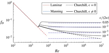
Variation of the friction factor versus the Reynolds number
 $Re$
and roughness parameter
 ${\it\epsilon}/(2w)=\{0.05,10^{-2},10^{-3},10^{-4}\}$
. The solid black lines indicate the predictions of (3.1), the dashed blue lines indicate the predictions of (3.2), the red dashed line shows the solution for laminar flow, while the dashed black line indicates the solution (3.1) for the case of no roughness, i.e.
 ${\it\epsilon}=0$
.

To illustrate the variation of the friction factor, figure 1 plots
 $f_{D}$
versus the Reynolds number
 $Re$
for different values of the roughness. The black solid lines and dashed blue lines indicate the predictions of (3.1) and (3.2) respectively for
 ${\it\epsilon}/(2w)=\{0.05,10^{-2},10^{-3},10^{-4}\}$
, while the black dashed line shows the prediction of (3.1) for
 ${\it\epsilon}=0$
. The laminar flow solution is shown by the dashed red line. As can be observed from the figure, estimates that are based on (3.1) first follow the laminar solution until
 $Re\lesssim 2000$
, then transition to the turbulent regime, and, finally, reach a plateau (all except
 ${\it\epsilon}=0$
). The relation (3.2) captures the plateau values for
 $10^{-3}\leqslant {\it\epsilon}/(2w)\leqslant 0.05$
and large
 $Re$
, but does not coincide with (3.1) for smaller values of the roughness or smaller
 $Re$
. At the same time, (3.1) captures both limiting cases, and therefore is more suitable as a universal model for describing flow in fractures where both laminar and turbulent flow regimes may occur within the same fracture.
For the purpose of hydraulic fracture modelling, it is convenient to factor the ‘laminar’ term in (3.1) as
 $$\begin{eqnarray}\displaystyle f_{D}=\frac{96}{Re}\tilde{f}_{D},\quad \tilde{f}_{D}(Re,r)=(1+(\tilde{A}+\tilde{B})^{-1.5})^{1/12}, & & \displaystyle\end{eqnarray}$$
where the new parameters are
 $$\begin{eqnarray}\displaystyle \tilde{A}=\left[\frac{8.511}{Re^{1/2}}f_{0}(Re,r)\right]^{16},\quad \tilde{B}=\left(\frac{2566}{Re}\right)^{24},\quad Re=\frac{2{\it\rho}Uw}{{\it\mu}},\quad r=\frac{{\it\epsilon}}{2w}. & & \displaystyle\end{eqnarray}$$
By substituting (3.3) into (2.1), one finds that
 $$\begin{eqnarray}\displaystyle U=-\frac{w^{2}}{12{\it\mu}\tilde{f}_{D}(Re,r)}\frac{\partial p}{\partial x}. & & \displaystyle\end{eqnarray}$$
Due to the factorization of the ‘laminar’ term (3.3), (3.5) appears to be similar to its counterpart for laminar flow. The only difference is the multiplier
 $\tilde{f}_{D}$
, which effectively changes the value of the viscosity depending on
 $Re$
and
 $r$
. It should be noted, however, that
 $\tilde{f}_{D}$
depends on the velocity, in which case (3.5) is an implicit equation for the velocity.
4 Tip region of hydraulic fractures with turbulent flow
4.1 Problem formulation
In order to better understand the influence of turbulent flow inside a hydraulic fracture, the aim of this section is to analyse the tip region of a hydraulic fracture in situations where the fluid flow can become turbulent. The tip region of a hydraulic fracture is known to obey a multiscale behaviour even without turbulence (Garagash, Detournay & Adachi Reference Garagash, Detournay and Adachi2011; Dontsov & Peirce Reference Dontsov and Peirce2015), while the addition of turbulence will enable one to better understand the transition from a laminar to a turbulent solution.
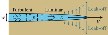
As follows from Garagash et al. (Reference Garagash, Detournay and Adachi2011), the problem of the tip region is equivalent to analysing a semi-infinite hydraulic fracture that propagates steadily in plane strain elastic conditions. With reference to figure 2, the volume balance for a steady semi-infinite hydraulic fracture that propagates with the velocity
 $V$
can be written as (see, e.g., Peirce & Detournay Reference Peirce and Detournay2008; Garagash et al.
Reference Garagash, Detournay and Adachi2011)
 $$\begin{eqnarray}\displaystyle U=V+2C^{\prime }V^{1/2}\frac{x^{1/2}}{w}, & & \displaystyle\end{eqnarray}$$
where
 $U$
is the mean fluid velocity inside the fracture,
 $C^{\prime }=2C_{L}$
is the scaled Carter leak-off coefficient, while
 $w$
is the fracture aperture. The fluid velocity and fluid pressure are related through the flow (3.5) as (the flow is in the negative
 $x$
direction)
 $$\begin{eqnarray}\displaystyle U=\frac{w^{2}}{{\it\mu}^{\prime }\tilde{f}_{D}(Re,r)}\frac{\text{d}p}{\text{d}x}, & & \displaystyle\end{eqnarray}$$
where
 ${\it\mu}^{\prime }=12{\it\mu}$
is the scaled fluid viscosity and
 $\tilde{f}_{D}(Re,r)$
is given in (3.3). An elasticity equation that automatically satisfies the linear elastic fracture mechanics solution at the fracture tip can be written as (Dontsov & Peirce Reference Dontsov and Peirce2015)
 $$\begin{eqnarray}\displaystyle w=\frac{K^{\prime }}{E^{\prime }}x^{1/2}-\frac{4}{{\rm\pi}E^{\prime }}\int _{0}^{\infty }F(x,s)\frac{\text{d}p}{\text{d}s}\,\text{d}s,\quad F(x,s)=(s-x)\ln \left|\frac{x^{1/2}+s^{1/2}}{x^{1/2}-s^{1/2}}\right|-2x^{1/2}s^{1/2}, & & \displaystyle \nonumber\\ \displaystyle & & \displaystyle\end{eqnarray}$$
where
 $K^{\prime }=\sqrt{32/{\rm\pi}}K_{Ic}$
,
 $K_{Ic}$
denotes the fracture toughness and
 $E^{\prime }=E/(1-{\it\nu}^{2})$
is the plane strain Young’s modulus.
Schematics of a semi-infinite plane strain brittle hydraulic fracture with leak-off and turbulent flow.

By following Dontsov & Peirce (Reference Dontsov and Peirce2015) and introducing the scaling
 $$\begin{eqnarray}\displaystyle \tilde{w}=\frac{E^{\prime }w}{K^{\prime }x^{1/2}},\quad {\it\chi}=\frac{2C^{\prime }E^{\prime }}{V^{1/2}K^{\prime }},\quad \tilde{x}=(x/l)^{1/2},\quad \tilde{s}=(s/l)^{1/2},\quad l=\left(\frac{K^{\prime 3}}{{\it\mu}^{\prime }E^{\prime 2}V}\right)^{2}, & & \displaystyle \nonumber\\ \displaystyle & & \displaystyle\end{eqnarray}$$
where
 $l$
is the length scale and the dimensionless parameter
 ${\it\chi}$
characterizes the leak-off, the governing equations (4.1)–(4.3) can be reduced to
 $$\begin{eqnarray}\displaystyle \tilde{w}(\tilde{x})=1+\frac{8}{{\rm\pi}}\int _{0}^{\infty }G\left(\frac{\tilde{s}}{\tilde{x}}\right)\tilde{f}_{D}\left[\frac{1}{\tilde{w}(\tilde{s})^{2}}+\frac{{\it\chi}}{\tilde{w}(\tilde{s})^{3}}\right]\text{d}\tilde{s},\quad G(t)=\frac{1-t^{2}}{t}\ln \left|\frac{1+t}{1-t}\right|+2. & & \displaystyle \nonumber\\ \displaystyle & & \displaystyle\end{eqnarray}$$
The primary difference between the formulation in Dontsov & Peirce (Reference Dontsov and Peirce2015) and (4.5) is the presence of the multiplier
 $\tilde{f}_{D}(Re,r)$
, which captures the effect of turbulent fluid flow. It should be noted that the Reynolds number and roughness parameter (3.4) can be written using (4.4) as
 $$\begin{eqnarray}\displaystyle Re=\tilde{Re}(\tilde{w}+{\it\chi})\tilde{s},\quad r=\frac{\tilde{r}}{\tilde{s}\tilde{w}},\quad \tilde{Re}=\frac{24{\it\rho}K^{\prime 4}}{{\it\mu}^{\prime 2}E^{\prime 3}},\quad \tilde{r}=\frac{{\it\epsilon}{\it\mu}^{\prime }E^{\prime 3}V}{2K^{\prime 4}}. & & \displaystyle\end{eqnarray}$$
The phenomenological model for turbulent flow (3.3) applies for all Reynolds numbers and
 $r\lesssim 0.05$
. In this situation, large variations of the Reynolds number in (4.6) are admissible, while large variations of the roughness parameter are not permitted. At the same time, the roughness does not noticeably influence the laminar flow in the adopted model (3.3) (see figure 1), and therefore large values of
 $r$
are permitted as soon as the flow is not turbulent. To provide a quick estimate for the case of no leak-off (in which case
 $U=V$
), one can calculate the value of
 $r$
from (3.4) as
 $$\begin{eqnarray}\displaystyle r=\frac{{\it\epsilon}{\it\rho}V}{{\it\mu}Re}. & & \displaystyle\end{eqnarray}$$
By substituting
 $Re=2000$
(just before the transition to turbulent flow),
 $V=1~\text{m}~\text{s}^{-1}$
,
 ${\it\epsilon}=10^{-4}$
m, and the properties of water
 ${\it\rho}=10^{3}~\text{kg}~\text{m}^{-3}$
,
 ${\it\mu}=10^{-3}$
Pa s into (4.7), one obtains
 $r=0.05$
. This shows that care must be taken when applying this approach to make sure that the model is not used beyond its applicability region.
4.2 Estimation of the laminar zone size
In order to estimate the influence of turbulence, it is instructive to know at what distance away from the fracture tip the turbulent effects become important. To this end, (4.6) can be rewritten as
 $$\begin{eqnarray}\displaystyle \frac{Re}{\tilde{Re}}=(\tilde{w}(\tilde{x},{\it\chi})+{\it\chi})\tilde{x}. & & \displaystyle\end{eqnarray}$$
Here,
 $\tilde{w}(\tilde{x},{\it\chi})$
should be a solution of (4.5) for laminar flow, i.e.
 $\tilde{f}_{D}=1$
, since the turbulence becomes important only some distance away from the tip. To produce a rapid estimate, one can use a closed-form approximate solution of (4.5) for
 $\tilde{f}_{D}=1$
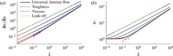
, which has been obtained in Dontsov & Peirce (Reference Dontsov and Peirce2015). Figure 3 shows the variation of
 $Re/\tilde{Re}$
versus
 $\tilde{x}$
that is calculated based on (4.8) and using the approximate width solution (referred to as the universal solution for laminar flow) from Dontsov & Peirce (Reference Dontsov and Peirce2015). The figure also shows the variation of the aforementioned approximate solution
 $\tilde{w}$
versus the normalized spatial coordinate
 $\tilde{x}$
. The values of the leak-off parameter used for the plot are
 ${\it\chi}=\{0,1,10,10^{2},10^{3}\}$
. The curves that correspond to larger values of
 ${\it\chi}$
are above those that represent smaller values of
 ${\it\chi}$
, which applies to both panels.
Variation of
 $Re/\tilde{Re}$
(4.8) (a) and
 $\tilde{w}$
(b) versus
 $\tilde{x}$
for
 ${\it\chi}=\{0,1,10,10^{2},10^{3}\}$
(solid black lines). The fracture width solution shown in (b) is calculated using an approximation obtained by Dontsov & Peirce (Reference Dontsov and Peirce2015). The dashed coloured lines indicate the vertex solutions (4.9).

The dashed red, blue and green lines correspond to the vertex solutions (asymptotic solutions of (4.5) for laminar flow
 $\tilde{f}_{D}=1$
, see, e.g., Garagash et al. (Reference Garagash, Detournay and Adachi2011)), which are given in the scaled form (4.4) by
 $$\begin{eqnarray}\displaystyle \tilde{w}_{k}=1,\quad \tilde{w}_{\tilde{m}}={\it\beta}_{\tilde{m}}{\it\chi}^{1/4}\tilde{x}^{1/4},\quad \tilde{w}_{m}={\it\beta}_{m}\tilde{x}^{1/3}, & & \displaystyle\end{eqnarray}$$
where the constants are
 ${\it\beta}_{\tilde{m}}=4/(15^{1/4}(\sqrt{2}-1)^{1/4})$
and
 ${\it\beta}_{m}=2^{1/3}3^{5/6}$
,
 $\tilde{w}_{k}$
stands for the toughness solution,
 $\tilde{w}_{m}$
represents the viscous solution and
 $\tilde{w}_{\tilde{m}}$
corresponds to the leak-off solution. As can be seen from figure 3, the estimation of the normalized Reynolds number from the leak-off solution (green dashed line in a) coincides with the results of the corresponding toughness and viscous solutions. This occurs because
 $1/\tilde{w}^{2}\ll {\it\chi}/\tilde{w}^{3}$
(or
 ${\it\chi}\gg \tilde{w}$
) in the leak-off regime (see (4.5) and discussion in Dontsov & Peirce (Reference Dontsov and Peirce2015)), which leads to
 $Re/\tilde{Re}=(\tilde{w}+{\it\chi})\tilde{x}\approx {\it\chi}\tilde{x}$
. This shows that the estimate of the normalized Reynolds number is independent of the fracture opening solution for the leak-off regime. As a result, one can use the ‘
 $mk$
’ solution (which is the no-leak-off laminar solution of (4.5), i.e.
 ${\it\chi}=0$
and
 $\tilde{f}_{D}=1$
) in (4.8) for the purpose of obtaining a crude estimate, i.e.
 $Re/\tilde{Re}=(\tilde{w}_{mk}+{\it\chi})\tilde{x}$
. The latter estimate for
 $Re/\tilde{Re}$
captures the small-leak-off case accurately, while the large-leak-off limit is captured automatically as discussed above. It should be noted that such an approximation (replacing
 $\tilde{w}$
by
 $\tilde{w}_{mk}$
in (4.8)) causes only a 10 % error in
 $Re/\tilde{Re}$
values for the range of parameters shown in figure 3. To simplify the calculations, the ‘
 $mk$
’ solution can be approximated as
 $\tilde{w}_{mk}\approx (1+{\it\beta}_{m}^{3}\tilde{x})^{1/3}$
, which introduces an additional error that is of the order of 1 %, see Dontsov & Peirce (Reference Dontsov and Peirce2015).
The procedure for estimating the size of the laminar zone can be formulated as follows. First, the fraction
 $Re/\tilde{Re}$
and leak-off parameter
 ${\it\chi}$
should be calculated based on the values of the problem parameters, and taking
 $Re=2000$
(turbulent effects become important for
 $Re\gtrsim 2000$
). Then, figure 3 can be used to calculate
 $\tilde{x}$
, which can be converted to a physical length using (4.4) as
 $d=l\tilde{x}^{2}$
. For instance, by taking
 $K_{Ic}=0.16~\text{MPa}~\text{m}^{1/2}$
,
 $E^{\prime }=6.8$
GPa,
 ${\it\rho}=1000~\text{kg}~\text{m}^{-3}$
,
 $C^{\prime }=0$
,
 ${\it\mu}=1.8\times 10^{-3}~\text{Pa}~\text{s}$
and
 $V=2~\text{m}~\text{s}^{-1}$
, which correspond to the parameters used in Tsai & Rice (Reference Tsai and Rice2010) for modelling glacial cracks, one obtains
 $d\approx 2$
m (
 $d\approx 5$
m if one accounts for the bi-material effect as in Tsai & Rice (Reference Tsai and Rice2010)). In other words, the size of the laminar zone is 2 m; however, this does not imply that the solution is turbulent immediately further away from the tip since there is always a transition zone. It should be noted that the size of the laminar zone strongly depends on the velocity, and for
 $V=0.5~\text{m}~\text{s}^{-1}$
(other parameters are kept the same) becomes
 $d\approx 30$
m. To address petroleum applications, consider a slick-water treatment with
 $K_{Ic}=1~\text{MPa}~\text{m}^{1/2}$
,
 $E^{\prime }=20$
GPa,
 ${\it\rho}=1000~\text{kg}~\text{m}^{-3}$
,
 $C^{\prime }=0$
,
 ${\it\mu}=10^{-3}$
Pa s and
 $V=1~\text{m}~\text{s}^{-1}$
. In this situation,
 $d\approx 7$
m. As expected, the size of the laminar zone also strongly depends on the viscosity, and for
 ${\it\mu}=10^{-1}$
Pa s one obtains
 $d\approx 730$
m. Therefore, no turbulence is expected near the tip. In order to provide similar estimates for different parameters, one may use figure 3 (and the procedure described in this section) to estimate the size of the laminar zone.
For simple fracture geometries, such as a plane strain or a radial fracture, the value of
 $d$
can be compared with the fracture length to quantify the global importance of the laminar tip. At the same time, for numerical schemes the value of
 $d$
needs to be compared with the size of the tip element, which would allow one to select a suitable asymptotic solution for calculations. For instance, if the element size is
 $1$
m, while
 $d=7$
m, then the laminar asymptotic solution should be used for the tip element to advance the fracture front even if turbulent flow develops further inside the fracture.
4.3 ‘Turbulent’ asymptotic solutions
This section focuses on calculating approximate solutions in situations where the effect of turbulent flow dominates the response. Two possibilities are considered: (i) a viscosity-dominated turbulent solution, labelled
 $\tilde{w}_{t}$
, and (ii) a leak-off-dominated turbulent solution, labelled
 $\tilde{w}_{\tilde{t}}$
. The corresponding governing equations can be obtained from (4.5) by retaining only the viscous or leak-off terms, and can be written respectively as
 $$\begin{eqnarray}\displaystyle \tilde{w}_{t}(\tilde{x})=\frac{8}{{\rm\pi}}\int _{0}^{\infty }G\left(\frac{\tilde{s}}{\tilde{x}}\right)\frac{\tilde{f}_{D}}{\tilde{w}_{t}^{2}}\,\text{d}\tilde{s},\quad \tilde{w}_{\tilde{t}}(\tilde{x})=\frac{8}{{\rm\pi}}\int _{0}^{\infty }G\left(\frac{\tilde{s}}{\tilde{x}}\right)\frac{{\it\chi}\tilde{f}_{D}}{\tilde{w}_{\tilde{t}}^{3}}\,\text{d}\tilde{s}. & & \displaystyle\end{eqnarray}$$
It should be noted that there is no toughness-dominated turbulent solution since for the latter the flow does not affect the solution. The friction factor (3.3), reduced for the turbulent regime (
 $Re\gtrsim 3000$
), and the friction factor (3.2) can be written as
 $$\begin{eqnarray}\displaystyle \tilde{f}_{D}\approx \frac{Re}{8.511^{2}}(f_{0}(Re,r))^{-2},\quad \tilde{f}_{D,2}=1.88\times 10^{-3}r^{1/3}Re. & & \displaystyle\end{eqnarray}$$
Further, the Reynolds number (4.6) for the viscous turbulent solution can be reduced to
 $Re=\tilde{Re}\tilde{w}\tilde{s}$
, while its counterpart for the leak-off turbulent solution is
 $Re={\it\chi}\tilde{Re}\tilde{s}$
, and the roughness parameter is the same for both solutions,
 $r=\tilde{r}/(\tilde{s}\tilde{w})$
.
By seeking the solution in the form
 $\tilde{w}_{t}={\it\beta}_{t}\tilde{x}^{{\it\gamma}}$
, the substitution of (4.11) into (4.10) leads to the following expressions for the viscosity-dominated and leak-off-dominated turbulent solutions for both friction factors in (4.11):
 $$\begin{eqnarray}\displaystyle \left.\begin{array}{@{}c@{}}\displaystyle \tilde{w}_{t}={\it\beta}_{t}\tilde{x},\quad {\it\beta}_{t}=0.4165\tilde{Re}^{1/2}\left[f_{0}\left(\tilde{Re}{\it\beta}_{t,0}\tilde{x}^{2},\frac{\tilde{r}}{{\it\beta}_{t,0}\tilde{x}^{2}}\right)\right]^{-1},\quad {\it\beta}_{t,0}\approx 0.08\tilde{Re}^{1/2},\\ \displaystyle \tilde{w}_{t,2}={\it\beta}_{t,2}\tilde{x}^{5/7},\quad {\it\beta}_{t,2}=0.221\tilde{Re}^{3/7}\tilde{r}^{1/7},\\ \displaystyle \!\!\!\tilde{w}_{\tilde{t}}={\it\beta}_{\tilde{t}}\tilde{x}^{1/2},\quad {\it\beta}_{\tilde{t}}=0.737\tilde{Re}^{1/4}{\it\chi}^{1/2}\left[f_{0}\!\left(\!{\it\chi}\tilde{Re}\tilde{x},\frac{\tilde{r}}{{\it\beta}_{\tilde{t},0}\tilde{x}^{5/3}}\right)\right]^{-1/2},\quad {\it\beta}_{\tilde{t},0}\approx 0.33\tilde{Re}^{1/4}{\it\chi}^{1/4},\\ \displaystyle \tilde{w}_{\tilde{t},2}={\it\beta}_{\tilde{t},2}\tilde{x}^{5/13},\quad {\it\beta}_{\tilde{t},2}=0.504\tilde{Re}^{3/13}{\it\chi}^{6/13}\tilde{r}^{1/13},\end{array}\right\} & & \displaystyle \nonumber\\ \displaystyle & & \displaystyle\end{eqnarray}$$
where the additional subscript ‘
 $2$
’ refers to the case where the second approximation for the friction factor in (4.11) is used (solutions with no additional subscript utilize the first approximation), the viscosity-dominated turbulent solutions are labelled with the subscript ‘
 $t$
’ and the leak-off-dominated turbulent solutions are augmented with the subscript ‘
 $\tilde{t}$
’. Here, the logarithmic term is treated as a slowly varying function, and the numeric factors in
 ${\it\beta}_{t,0}$
and
 ${\it\beta}_{\tilde{t},0}$
are calculated from estimating
 $|0.9\log (7/Re)|$
for
 $Re=2000$
.
It should be noted that the unscaled solutions, which can be calculated from (4.12) using the scaling (4.4), vary with distance as
 $w_{t}\propto x$
,
 $w_{t,2}\propto x^{6/7}$
,
 $w_{\tilde{t}}\propto x^{3/4}$
and
 $w_{\tilde{t},2}\propto x^{9/13}$
. It should also be noted that the solution
 $\tilde{w}_{t,2}$
(4.12) is consistent with the one used in Tsai & Rice (Reference Tsai and Rice2010), where the latter was calculated based on the solution for a power-law fluid (Desroches et al.
Reference Desroches, Detournay, Lenoach, Papanastasiou, Pearson, Thiercelin and Cheng1994). In order to obtain identical agreement one needs to remove the bi-material effect from the solution by Tsai & Rice (Reference Tsai and Rice2010), and to account for the numerical factors appearing in the expressions for
 $\tilde{Re}$
and
 $\tilde{r}$
in (4.6).
4.4 Numerical solution
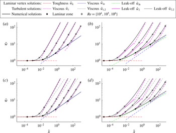
To illustrate the applicability of the laminar zone size estimate covered in § 4.2 and the ‘turbulent’ asymptotic solutions described in § 4.3, figure 4 shows the numerical solutions of (4.5) for various parameters. In particular, the solutions are calculated for the normalized Reynolds numbers
 $\tilde{Re}=\{0,10,10^{3},10^{5},10^{7}\}$
, for leak-off parameter
 ${\it\chi}=0$
and
 ${\it\chi}=10$
, and for normalized roughness
 $\tilde{r}=0$
and
 $\tilde{r}=60/\tilde{R}e$
. The latter choice for the roughness is based on the estimate (4.7), for which
 $r=0.03$
is chosen, and ensures that the adopted model is not used beyond its applicability region. It should be noted that the aforementioned estimate is valid for the no-leak-off case and becomes an approximation for the case
 ${\it\chi}=10$
. The estimate of the laminar zone size that is based on (4.8), the vertex asymptotic solutions (4.9) and the ‘turbulent’ asymptotic solutions (4.12) are all shown as well.
Numerical solutions of (4.5) calculated using (3.3) for
 $\tilde{Re}=\{0,10,10^{3},10^{5},10^{7}\}$
(solid black lines). The lowest curve in each panel corresponds to the purely laminar solution (
 $\tilde{Re}=0$
), while the highest curves represent the
 $\tilde{Re}=10^{7}$
cases. The (a,c) solutions without leak-off, i.e.
 ${\it\chi}=0$
; (b,d) solutions for
 ${\it\chi}=10$
. (a,b) Solutions in smooth fractures, for which the roughness is zero, i.e.
 $\tilde{r}=0$
; (c,d) solutions for which the roughness is calculated as
 $\tilde{r}=60/\tilde{R}e$
. The estimate of the laminar zone size, based on (4.8), is highlighted by the black filled circular markers. The vertex asymptotic solutions (4.9) are indicated by dashed red, blue and green lines, while the ‘turbulent’ asymptotic solutions (4.12) are indicated by dashed and solid magenta and grey lines. The square markers indicate the locations at which the Reynolds numbers associated with the flow in the fracture are
 $Re=\{10^{4},10^{5},10^{6}\}$
.

As can be seen from figure 4, larger values of
 $\tilde{Re}$
correspond to situations in which turbulent effects occur closer to the tip. The solution may ‘depart’ from either one of the vertex solutions (4.9) (dashed red, blue and green lines), or from a transition zone between the aforementioned solutions. The estimate of the laminar zone size (4.8) is able to estimate the validity of the laminar solution accurately for almost all cases. One exception is when the turbulent flow occurs while hydraulic fracture is propagating in the toughness regime. For the latter case, the estimate (4.8) is on the safe side, as it underestimates the validity region of the laminar solution. It should be noted that this occurs because the fluid flow does not affect the solution in the toughness regime, so that one can use the toughness solution even if the flow is turbulent. The ‘turbulent’ asymptotic solutions (4.12) calculated using (3.3),
 $\tilde{w}_{t}$
, and
 $\tilde{w}_{\tilde{t}}$
, provide a reasonably accurate estimate as soon as they apply. It should be noted that the accuracy is smaller than for the vertex solutions, which is due to additional approximations associated with the logarithmic term. On the other hand, the asymptotic solutions based on (3.2),
 $\tilde{w}_{t,2}$
and
 $\tilde{w}_{\tilde{t},2}$
, do not apply for smooth fractures, while they provide a good estimate for rough fractures. This is consistent with the results shown in figure 1, where both models give similar values for the friction factor in the range
 $10^{-3}<{\it\epsilon}/(2w)<5\times 10^{-2}$
. It should be noted that the roughness parameter becomes smaller for wider fractures, in which case the solutions
 $\tilde{w}_{t,2}$
and
 $\tilde{w}_{\tilde{t},2}$
inevitably divert from the numerical solutions. It should also be noted that all leak-off asymptotes require
 ${\it\chi}\gg 1$
, while relatively modest
 ${\it\chi}=10$
is used for plotting figure 4(b,d). For this reason, there is an additional discrepancy between the numerical solution and the asymptotes.
Since elasticity produces a non-local effect and there is a transition zone between laminar and fully developed turbulent flows, the turbulent asymptotic solutions do no apply immediately after the flow becomes non-laminar. There is a transition zone, which, according to figure 4, occurs approximately until
 $Re\gtrsim 10^{4}$
(the values are larger for solutions ‘departing’ from the toughness asymptote). Due to the presence of the transition zone, the estimate of the laminar zone size, described in § 4.2, cannot be used directly to quantify the distance from the fracture tip after which the turbulent asymptotic solution can be applied. In order to have a better estimate, one should multiply the calculated laminar zone size
 $\tilde{x}$
by a factor of 3–5 (this corresponds to the distance between the circular marker and the first square marker), in which case the final answer becomes at least an order of magnitude larger due to the scaling (4.4) since
 $x\propto \tilde{x}^{2}$
. This again shows that care must be taken when using turbulent flow models and the associated asymptotic solutions for hydraulic fracture modelling to make sure that the solutions are not used beyond their applicability region.
5 Summary
This study has investigated the effect of turbulent fluid flow on the near-tip behaviour of hydraulic fractures. First, the phenomenological formula that describes fluid flow in pipes has been adapted to quantify fluid flow in fractures. This flow model is able to capture the viscous fluid resistance in situations where the flow is laminar, turbulent or in the transition zone. Then, the turbulent flow model has been applied to analyse the steady propagation of a semi-infinite hydraulic fracture. An estimate of the laminar zone size within which the classical laminar flow multiscale solution applies has been obtained. Expressions for asymptotic solutions that are associated with fully developed turbulent flow inside the hydraulic fracture have been derived. A multiscale numerical solution for a semi-infinite hydraulic fracture, for which the flow changes from laminar near the tip to fully turbulent away from the tip, has been obtained by using a non-singular integral equation formulation. The numerical solutions have been compared with the asymptotic solutions for laminar and turbulent flow, and the estimate of the laminar zone size has been verified.