





Impact statement
Dryland livestock systems in the Paraguayan Chaco are rapidly expanding into drier, more fragile landscapes, but the field measurements needed to detect early pasture decline and emerging soil salinity are still scarce and costly to obtain at scale. This study provides a practical, low-cost early warning screening approach that uses freely available multispectral satellites and cloud computing to (1) map bare soil “peladares” during peak greenness and (2) track two decades of vegetation change alongside indicators of plant water stress and evapotranspiration dynamics. By separating land-use history effects from within-cohort degradation signals and ranking multiple salinity indices against year-adjusted vegetation decline, we identify an informative proxy (SI6) to prioritize where on-the-ground soil and groundwater monitoring should happen first.
Introduction
Soil salinization is currently one of the major environmental and socioeconomic threats worldwide, already affecting ~8.3 million km2 (Hassani et al., Reference Hassani, Azapagic and Shokri2021). Salinity reduces plant water uptake through osmotic stress, imposes ionic stress that triggers toxicity and can impair soil structure and nutrient cycling; together, these effects rapidly constrain agricultural productivity and ecosystem functioning (Shelden and Munns, Reference Shelden and Munns2023). Climate change is expected to exacerbate the problem, particularly in drylands such as the Great South American Chaco, a recognized salinization hotspot. This biome forms one of the world’s largest and flattest sedimentary plains, bordered by the Andes to the west and the Brazilian Shield to the north and east. Characterized by subhumid to semiarid climates, the region has received significant Andean deposits, such as loess and volcanic ash, shaped during the Late Quaternary by both aeolian and alluvial processes (Sayago et al., Reference Sayago, Collantes, Karlson and Sanabria2001). Evidence of salinization, especially in the Argentinian Chaco, has been documented through indicators such as elevated soil and groundwater electrical conductivity, shallow water tables, salt crust and vegetation composition (Marchesini et al., Reference Marchesini, Giménez, Nosetto and Jobbágy2017; Jobbágy et al., Reference Jobbágy, Giménez, Marchesini, Diaz, Jayawickreme, Nosetto, Taleisnik and Lavado2020).
In particular, the current land-use change dynamic in the Paraguayan Chaco is marked by a rapid acceleration of deforestation, with the deforested area between 2001 and 2012 doubling relative to the 1987–2000 period (Baumann et al., Reference Baumann, Piquer-Rodríguez, Fehlenberg, Gavier Pizarro, Kuemmerle, Niewöhner, Bruns, Hostert, Krueger, Nielsen, Haberl, Lauk, Lutz and Müller2016; Baumann et al., Reference Baumann, Israel, Piquer-Rodríguez, Gavier-Pizarro, Volante and Kuemmerle2017; Milán et al., Reference Milán, González and López-i-Gelats2024), a trend further confirmed by the most recent national report estimating an annual loss of ~180,000 ha between 2017 and 2021 (INFONA, 2023), and nearly 300.000 ha lost from 2022 to 2024 (INFONA, 2026). Alongside this, the advance of agriculture is reshaping land pressures occurring within a region where aridity strongly conditions land suitability. Although Houspanossian et al. (Reference Houspanossian, Giménez, Baldi and Nosetto2016) found no clear association between overall deforestation and the aridity gradient, they reported that 90% of new crops established between 2001 and 2012, predominantly involving pasture replacement, were concentrated in low- and medium-aridity areas, while new pasture expanded toward drier zones, indicating a displacement of livestock production into more marginal environments. More recently, Henderson et al. (Reference Henderson, Godar, Frey, Börner and Gardner2021) described the potential of the Paraguayan Chaco to become a large-scale soybean production region, identifying ~940,000 ha as moderately suitable for agricultural expansion.
Australia offers one of the clearest examples of how replacing native dry forest with crops and pasture can trigger severe dryland salinity. By 1980, nearly 40% of these ecosystems had been cleared, and in the southwest alone, more than 2 million hectares of productive land became salt-affected. This large-scale salinization highlights how strongly native vegetation regulates water dynamics and how human-driven cover change can rapidly destabilize them (Lambers, Reference Lambers2003; Bradshaw, Reference Bradshaw2012). According to Marchesini et al. (Reference Marchesini, Giménez, Nosetto and Jobbágy2017), the comparison between Australia and Argentina’s Dry Chaco shows that both regions experience substantial increases in deep drainage following the conversion of dry forests to agriculture, with Chaco sites exhibiting more than double the deep soil water of native stands and recharge rates up to two orders of magnitude higher. These patterns resemble the early stages of salinization documented in Australia, though the Chaco’s lower salt deposition, younger sediments and higher water-use crops temper the overall risk. Nevertheless, its extremely flat topography and shallow water tables could allow recharge and salt mobilization to propagate more extensively, creating management challenges that may parallel, but remain less severe than, the Australian case. Moreover, Jobbágy et al. (Reference Jobbágy, Giménez, Marchesini, Diaz, Jayawickreme, Nosetto, Taleisnik and Lavado2020) summarized studies carried out in the dry plains of southern South America and emphasized that while soil maps showed one-fourth of the region’s soil as saline, research in which the relation between soil-hydrology-vegetation and land-use change is considered, a much more widespread and dynamic salinization is reported. Together, these findings suggest that “secondary” (land-use driven) salinization can emerge as a hidden, spatially expanding process even where surface symptoms are still patchy.
Ecohydrological data and measurements of soil and groundwater electrical conductivity in the Paraguayan Chaco remain extremely limited, leaving major uncertainties regarding the extent and drivers of emerging salinization; nonetheless, several areas of the region have already been reported as showing clear symptoms of salinity impact, indicating that the process is underway despite the scarcity of systematic observations (Laino et al., Reference Laino, Neufeld and Glatzle2022). This evidence gap limits early warning and prioritization of field validation, particularly in departments undergoing rapid land conversion. As an initial step toward addressing this gap, this study provides a first assessment of pasture degradation and potential salinity-affected areas in the Boquerón department, Paraguay, using an affordable, multispectral remote sensing approach that integrates land-use change, vegetation cover and climatic conditions. Building on this baseline, we outline a potential pipeline to generate the scientific evidence currently lacking, including the development of a “secondary salinization prediction map” for the Paraguayan Chaco that combines ecohydrological indicators, soil cover, texture and electrical conductivity, with aridity index and groundwater attributes such as depth and salt content. Specifically, we aimed to (i) map pasture degradation and screen for areas potentially affected by abiotic stressors such as drought and salinity in Boquerón; (ii) outline a scalable framework to support a future secondary-salinization prediction map by integrating ecohydrological, soil, aridity and groundwater attributes; and (iii) generate a baseline screening product to prioritize hotspots for targeted in situ validation and monitoring.
Methods
Study area and analytical units
We conducted the analysis in a ~500,000 ha square region in the Department of Boquerón, western Paraguay (Chaco), selected for its central position within the Chaco region and proximity to the service hub of Mariscal Estigarribia. Spatial analyses were implemented using a common 500 m grid, and cartographic products were also presented in WGS84 geographic coordinates (EPSG:4326). The primary analytical unit for statistical inference was the bare soil polygon, detected using a supervised random forest classification (see below), with polygon area (ha) used as an explicit weight in aggregation and modeling to account for unequal polygon sizes.
Land-use history and cohort definition
We characterized land-use history using the Hansen Global Forest Change product (tree cover baseline year 2000 and annual forest loss), accessed through Google Earth Engine (GEE), a cloud-based platform for large-scale geospatial analysis (Hansen et al., Reference Hansen, Potapov, Moore, Hancher, Turubanova, Tyukavina, Thau, Stehman, Goetz, Loveland, Kommareddy, Egorov, Chini, Justice and Townshend2013; Gorelick et al., Reference Gorelick, Hancher, Dixon, Ilyushchenko, Thau and Moore2017). Baseline forest in 2000 was defined as pixels with tree cover ≥30% (treecover2000) and filtered for minimum patch connectivity using a connected-pixel criterion (minimum six connected pixels). Pixels experiencing forest loss were assigned to the corresponding calendar year of loss (loss year +2000), persistent forest (no recorded loss) was coded as 2025 and areas that were never forest in the baseline mask were coded as 99 (later recorded to 1999 as a stable non-forest reference class during downstream analysis). The last-year-of-cover layer was aggregated to 500 m using a modal reducer to preserve categorical meaning.
For interpretability, we summarized land-use history into cohort bins reflecting broad conversion periods (e.g., stable non-forest, 2001–2005, 2006–2010, 2011–2015, 2016–2020, 2021–2024 and stable forest) and used these cohorts to color/label visual diagnostics and summary plots.
Peladares (bare soils) detection 2025
We implemented all satellite data preprocessing, spectral index computation and pixel-level sampling in GEE to identify peladares , defined as areas with low plant cover (Zeballos et al., Reference Zeballos, ATR, Agüero, Ahumada, Almirón, Argibay, Arroyo, Blanco, Biurrun, Cantero, Márquez, Quiroga, Quiroga and Cabido2023). We focused on the peak-greenness period (1 April–15 July 2025) to minimize confusion between seasonal senescence and true bare or degraded surfaces. Similar remote-sensing-based approaches have been applied to map bare and degraded land surfaces in other dryland systems (Zhang et al., Reference Zhang, Wu, Kang, Fan, Wang, Liu and He2024).
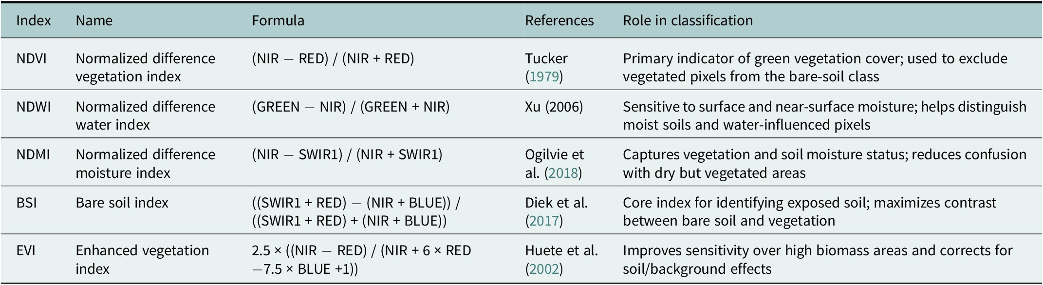
We performed an object-based supervised classification on Sentinel-2 imagery following multiresolution image segmentation, which grouped spectrally homogeneous pixels into image objects that served as the basic units of analysis. We constructed a multivariate feature set from spectral bands (BLUE, GREEN, RED, NIR, SWIR1 and SWIR2), spectral indices related to vegetation, moisture and soil conditions (NDVI, NDWI, NDMI, BSI and EVI) and elevation (see Table 1). For each image object, we computed the mean, standard deviation, maximum and minimum values of all predictors to capture within-object spectral variability and reduce pixel-level noise.
Spectral indices used as predictor variables in the supervised classification of peladares

Table 1. Long description
The table contains five columns and five rows of data.
Row 1: Index N D V I. Name: Normalized difference vegetation index. Formula: (N I R minus R E D) forward slash (N I R plus R E D). References: Tucker 1979. Role: Primary indicator of green vegetation cover; used to exclude vegetated pixels from the bare-soil class.
Row 2: Index N D W I. Name: Normalized difference water index. Formula: (G R E E N minus N I R) forward slash (G R E E N plus N I R). References: Xu 2006. Role: Sensitive to surface and near-surface moisture; helps distinguish moist soils and water-influenced pixels.
Row 3: Index N D M I. Name: Normalized difference moisture index. Formula: (N I R minus S W I R 1) forward slash (N I R plus S W I R 1). References: Ogilvie et al. 2018. Role: Captures vegetation and soil moisture status; reduces confusion with dry but vegetated areas.
Row 4: Index B S I. Name: Bare soil index. Formula: ((S W I R 1 plus R E D) minus (N I R plus B L U E)) forward slash ((S W I R 1 plus R E D) plus (N I R plus B L U E)). References: Diek et al. 2017. Role: Core index for identifying exposed soil; maximizes contrast between bare soil and vegetation.
Row 5: Index E V I. Name: Enhanced vegetation index. Formula: 2.5 times ((N I R minus R E D) forward slash (N I R plus 6 times R E D minus 7.5 times B L U E plus 1)). References: Huete et al. 2002. Role: Improves sensitivity over high biomass areas and corrects for soil/background effects.
We applied Random Forest-based feature selection before model fitting. The procedure retained all index-derived predictors, and we trained the final Random Forest classifier using the full joint feature set. The classification delineated bare soil polygons with an overall accuracy of 95%. These polygons subsequently defined the sampling frame for extracting long-term vegetation trend metrics (2000–2024) and salinity indices for 2025.
Remote sensing datasets and preprocessing
Normalized difference vegetation index time series (Landsat 7/8/9)
We estimated long-term vegetation change using Landsat Collection 2, Tier 1, Level-2 surface reflectance imagery (Landsat 7 ETM+, Landsat 8 OLI and Landsat 9 OLI-2). Surface reflectance bands were scaled using the Collection 2 coefficients (reflectance = DN × 0.0000275 − 0.2). Clouds, cirrus, cloud shadows, snow and radiometrically saturated pixels were masked using the QA_PIXEL and QA_RADSAT bands. Normalized Difference Vegetation Index (NDVI) was computed as the normalized difference of NIR and red reflectance, harmonized across sensors using sensor-appropriate band mappings. Within each year (2000–2024), we produced a per-year NDVI composite by taking the median of all valid observations within a user-defined intra-annual window (parameterized to represent the dry-season window in the Chaco). To quantify long-term trends while remaining robust to outliers and non-normality typical of remotely sensed time series, we estimated monotonic trends using Sen’s slope (Sen, Reference Sen1968). Sen’s slope was computed per pixel and then summarized by land-use cohort and by polygon-level area weighting. This trend method was applied to NDVI, CWSI and ET.
Land surface temperature and crop water stress index (MOD11A2)
We used MODIS Terra MOD11A2 (8-day, 1 km) daytime land surface temperature (LST_Day_1km). Land surface temperature (LST) values were converted to °C (LST × 0.02 − 273.15) and aggregated to monthly means, with missing observations retained as masked values. A simplified, remotely sensed Crop Water Stress Index (CWSI) was then derived, and long-term monotonic trends were estimated using Sen’s slope. The index was calculated using fixed wet and dry reference temperatures derived from the study region, defined as the 5th and 95th percentiles of long-term mean LST (T_w and T_d, respectively). This approach evaluates whether peladares exhibit elevated thermal water stress relative to the landscape, rather than representing true physiological water stress. Monthly CWSI was computed as:

Evapotranspiration (MOD16A2GF)
We used MODIS MOD16A2GF (8-day, ~500 m) evapotranspiration (ET) and applied the documented scale factor (ET × 0.1) to express ET in mm per 8-day period. The ET time series was constrained to the same intra-annual window as the NDVI/LST analyses (parameterized) and processed to a Sen-slope trend surface at the native 500 m scale.
Trend estimation with Sen’s slope
For NDVI, CWSI and ET, we quantified long-term monotonic change per pixel implemented through a Sen-slope reducer. Each series image was paired with an explicit time band (t) and reduced to obtain a slope parameter per pixel. To ensure reliability, NDVI trend estimation required a minimum number of annual observations (≥6 years with valid data). Trend surfaces were clipped to the region of interest and harmonized to a common 500 m grid for downstream polygon summaries.
Salinity indices (Landsat 8/9 composite, 2025)
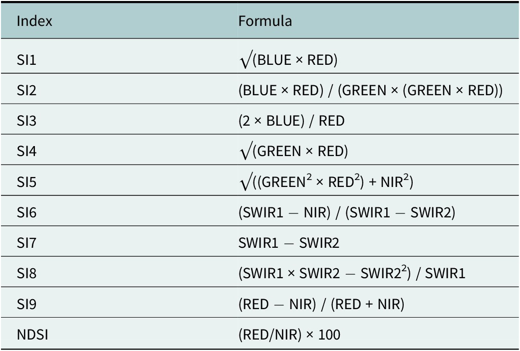
We calculated 10 salinity indices commonly used in optical remote sensing studies of salt-affected soils, following the formulations compiled by Zhang et al. (Table 2). To evaluate candidate indices within the peladar landscape, we built a Landsat 8/9 surface reflectance median composite for 1 April–15 July 2025 after applying QA-based cloud/shadow masking and standard reflectance scaling. We then computed SI1–SI9 and an NDSI-style ratio from band algebra using BLUE, GREEN, RED, NIR, SWIR1 and SWIR2. To improve numerical stability, we added a small epsilon to denominators to prevent division by near-zero values and constrained square-root terms by clamping negative products to zero. Finally, we aggregated the salinity-index stack to 500 m using a mean reducer so it aligned with the analysis grid and could be compared directly with the 500 m trend stack.
Salinity indices calculated and evaluated within peladar polygons

Table 2. Long description
The table consists of two columns: Index and Formula.
* S I 1: square root of (B L U E times R E D).
* S I 2: (B L U E times R E D) all over (G R E E N times (G R E E N times R E D)).
* S I 3: (2 times B L U E) all over R E D.
* S I 4: square root of (G R E E N times R E D).
* S I 5: square root of ((G R E E N super 2 times R E D super 2) plus N I R super 2).
* S I 6: (S W I R 1 minus N I R) all over (S W I R 1 minus S W I R 2).
* S I 7: S W I R 1 minus S W I R 2.
* S I 8: (S W I R 1 times S W I R 2 minus S W I R 2 super 2) all over S W I R 1.
* S I 9: (R E D minus N I R) all over (R E D plus N I R).
* N D S I: (R E D forward slash N I R) times 100.
Note: All indices were computed from atmospherically corrected surface reflectance bands and appended to each image for subsequent extraction and statistical analysis. Compiled by Zhang et al. (Reference Zhang, Wu, Kang, Fan, Wang, Liu and He2024).
Pixel sampling and polygon aggregation
We constructed a 500 m multiband stack comprising NDVI Sen slope, CWSI Sen slope, ET Sen slope and last-year-of-cover (categorical). We then sampled all 500 m pixels intersecting each peladar polygon using a sampleRegions function, preserving pixel geometry and attaching polygon metadata (poly_id and polygon area in ha). Salinity indices (500 m) were sampled using the same polygon set and joined to the trend stack at the pixel level using a unique pixel identifier. We summarized pixel-level values to one record per polygon by taking the median across all pixels within each polygon for each variable (NDVI slope, ET slope, CWSI slope, last-year-of-cover and each salinity index). Polygon area (ha) was carried forward and used as an analytical weight.
Removing cohort effects with GAMs and residualization
Because NDVI, CWSI, ET and several candidate salinity indices exhibited a strong shared dependence on time-since-conversion (cohort effects), we separated cohort-driven trajectories from within-cohort variation before ranking salinity indices. We modeled NDVI as a smooth function of year (and/or cohort age) using generalized additive models (GAMs), which are well-suited to nonlinear ecological time series and allow flexible smooth terms with principled penalization (Simpson, Reference Simpson2018). We used restricted maximum likelihood (REML) to estimate smoothing penalties.
To describe the dominant cohort effect associated with land-use history, we aggregated polygon-level metrics to a year-level table, where for each last-year-of-cover value we computed an area-weighted median across polygons. These year-level summaries were used to visualize baseline trajectories of NDVI, ET and CWSI versus land-use cohort using weighted GAMs.
To disentangle within-cohort vegetation degradation from cohort-driven baselines, we fit separate polygon-level, area-weighted GAMs for each trend metric:

where (y) is the NDVI Sen slope, ET Sen slope or CWSI Sen slope, and s(.) is a penalized spline fit with REML smoothing selection. We then computed year-adjusted residuals for each polygon as:

Mechanism checks among residuals
To evaluate whether year-adjusted vegetation change covaried with year-adjusted water stress and water flux, we quantified area-weighted Pearson correlations between NDVI residuals and ET residuals, and between NDVI residuals and CWSI residuals. Residuals represent polygon-level departures from the cohort-expected trend (observed minus GAM-predicted), isolating within-cohort variation in NDVI/ET/CWSI after accounting for land-use history. These relationships were also visualized with weighted GAM smooths to assess potential nonlinearity.
Ranking and selecting the “best” salinity index
We evaluated each candidate’s salinity index using two complementary, area-weighted criteria:
-
1. Association with year-adjusted NDVI degradation: area-weighted Pearson correlation between each salinity index and NDVI residuals (after removing the cohort effect).
-
2. Incremental predictive value beyond land-use history: improvement in area-weighted RMSE when adding the salinity index to the baseline NDVI model:

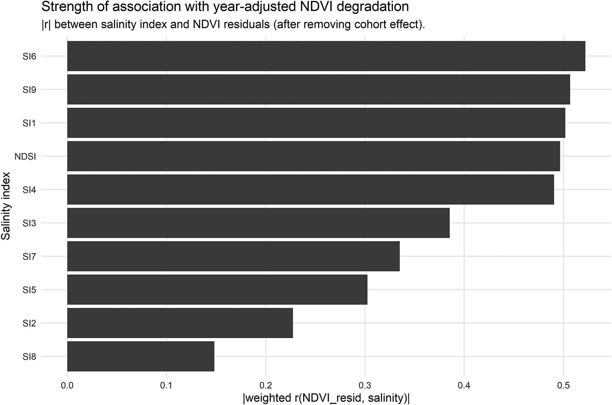
We computed ΔRMSEꙍ as RMSEꙍ (year-only) − RMSEꙍ(year + index), and used this as the primary ranking metric, with |r| as a secondary criterion to break ties. The full ranking and the diagnostic relationship for the top-ranked index are shown in Figure 3.
Long-term climatic control
To further understand if NDVI peladares dynamics are more reflective of local practices, the presence of permanent soil chemical changes or drought cycles, we modeled the relationship between annual mean precipitation derived from the CHIRPS dataset and Landsat surface reflectance using a GAM of the form:

where s() represents a smooth, nonlinear function. The model was fitted using REML, and model performance was evaluated using deviance explained. The significance of the smooth term was assessed using approximate F-tests.
Software and reproducibility
All remote sensing processing (masking, compositing, Sen-slope trend estimation, Hansen-derived land-use history and polygon-based pixel sampling) was implemented in GEE (JavaScript API). Statistical analyses, aggregation, GAM fitting and figure generation were performed in R using mgcv, dplyr, tidyr and ggplot2. Intermediate products (trend rasters, salinity-index rasters, pixel-level samples, polygon summaries and year summaries) were exported as GeoTIFF/CSV to enable fully traceable post-processing and replication.
Results and discussion
Land-use change dynamics in Chaco are driven by the rapid expansion of agriculture and livestock frontiers
The Paraguayan Chaco represents the country’s main frontier for agricultural expansion following the implementation of a zero-deforestation law in eastern Paraguay in 2004. Although land-use change is regulated by multiple legal frameworks, including mandatory forest retention, clearing limits, environmental impact assessments and the establishment of the Chaco Biosphere Reserve, deforestation and wildfires persist within and around protected areas, with forest-cover losses reaching up to 25% in some reserves and elevated deforestation rates in adjacent buffer zones (Da Ponte et al., Reference Da Ponte, García-Calabrese, Kriese, Cabral, Perez de Molas, Alvarenga, Salinas, Caceres, Gali, García, Morinigo and Ríos2021). The Boquerón department exhibits the highest deforestation rates in the region, with ~2.9 million ha of forest lost since 2001 (41% of the original cover) and over 90,000 ha cleared between 2021 and 2022 alone (INFONA, 2023). This trend is closely linked to rapid livestock-driven pasture expansion, with exotic pasture area increasing by 50.9% between 2008 and 2022, while Megathyrsus maximus cv. Gatton panic expanded by 142% regionally and by 987% in Boquerón (MAG, 2023). Together, these trends underscore the Chaco’s high vulnerability to land-cover change despite existing legal protections, emphasizing the need for targeted conservation and monitoring strategies.
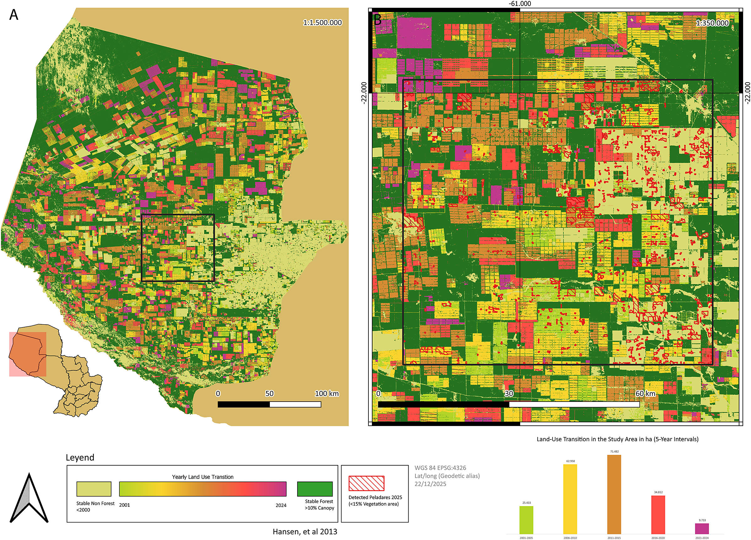
Therefore, we selected a 500,000 ha region in Boquerón due to its pronounced land-use change dynamics and status as a hotspot within the livestock expansion frontier, discussed above. This area was considered an ideal case study to assess the potential presence of degraded pastures and salt-affected soils, given the intensive conversion of native dry forests to pastures and crops, which may have altered the local hydrology, leading to degradation and early-stage salinization processes (Figure 1a).
Land-use change and study area in Boquerón Department, Paraguay. Deforestation dynamics, with colors representing 5-year intervals, with a square highlighting the study area (a). Detected peladares are highlighted in red (b).

Figure 1. Long description
A multi-panel figure containing two maps and a bar chart.
Panel A, on the left, is a large-scale map of Boquerón Department at 1:1,500,000 scale. A small inset map of Paraguay at the bottom-left shows the department’s location in the Northwest. The main map shows a mosaic of land use. Stable forest with greater than 10 percent canopy is concentrated in the North and West. The central and Eastern regions show a dense grid-like pattern of land-use transition. A black square in the center-South highlights the specific study area. A scale bar indicates 0 to 100 kilometers.
Panel B, on the right, is a zoomed-in map of the study area at 1:350,000 scale. It shows a high-density grid of rectangular land plots. Red outlines indicate detected peladares, which are areas with less than 15 percent vegetation. These red-outlined areas are scattered throughout the central and Eastern portions of the grid. A scale bar indicates 0 to 60 kilometers.
Below the maps is a legend. A color gradient for Yearly Land Use Transition ranges from yellow in 2001 to red in 2024. Light beige represents stable non-forest before 2000, and dark green represents stable forest.
At the bottom-right is a bar chart titled Land-Use Transition in the Study Area in ha 5-Year Intervals. The x-axis shows five time periods, and the y-axis represents area in hectares.
- 2001-2005: Green bar at 25,433.
- 2006-2010: Yellow bar at 61,958.
- 2011-2015: Orange bar at 71,482.
- 2016-2020: Red bar at 34,812.
- 2021-2024: Purple bar at 9,733.
The chart shows a peak in land-use transition during the 2011-2015 period followed by a decline.
Using multispectral satellite imagery, we classified the study area into four primary land-cover types: dry forest, cropland/grassland, open water and bare soil. Spectral bands and vegetation indices were used to optimize class separability (Baeza et al., Reference Baeza, Vélez-Martin, De Abelleyra, Banchero, Gallego, Schirmbeck, Veron, Vallejos, Weber, Oyarzabal, Barbieri, Petek, Guerra Lara, Sarrailhé, Baldi, Bagnato, Bruzzone, Ramos and Hasenack2022). A supervised classification approach was implemented using a Random Forest algorithm, which has demonstrated high robustness in heterogeneous dryland environments (Supplementary Figure 1). Training samples were derived from visually validated reference points and the model was applied to the full 500,000 ha region to generate a spatially explicit land-cover map for subsequent analyses (Figure 1b). In Figure 2a, areas classified as peladares (bare soils) are highlighted and interpreted as degraded land, characterized by a high percentage of bare soil or absent vegetation cover (Zeballos et al., Reference Zeballos, ATR, Agüero, Ahumada, Almirón, Argibay, Arroyo, Blanco, Biurrun, Cantero, Márquez, Quiroga, Quiroga and Cabido2023). Such conditions may arise from pasture degradation associated with unsustainable land-use practices (e.g., chronic overgrazing or inadequate management) and may be further exacerbated by abiotic stressors, including soil salinization and recurrent drought.
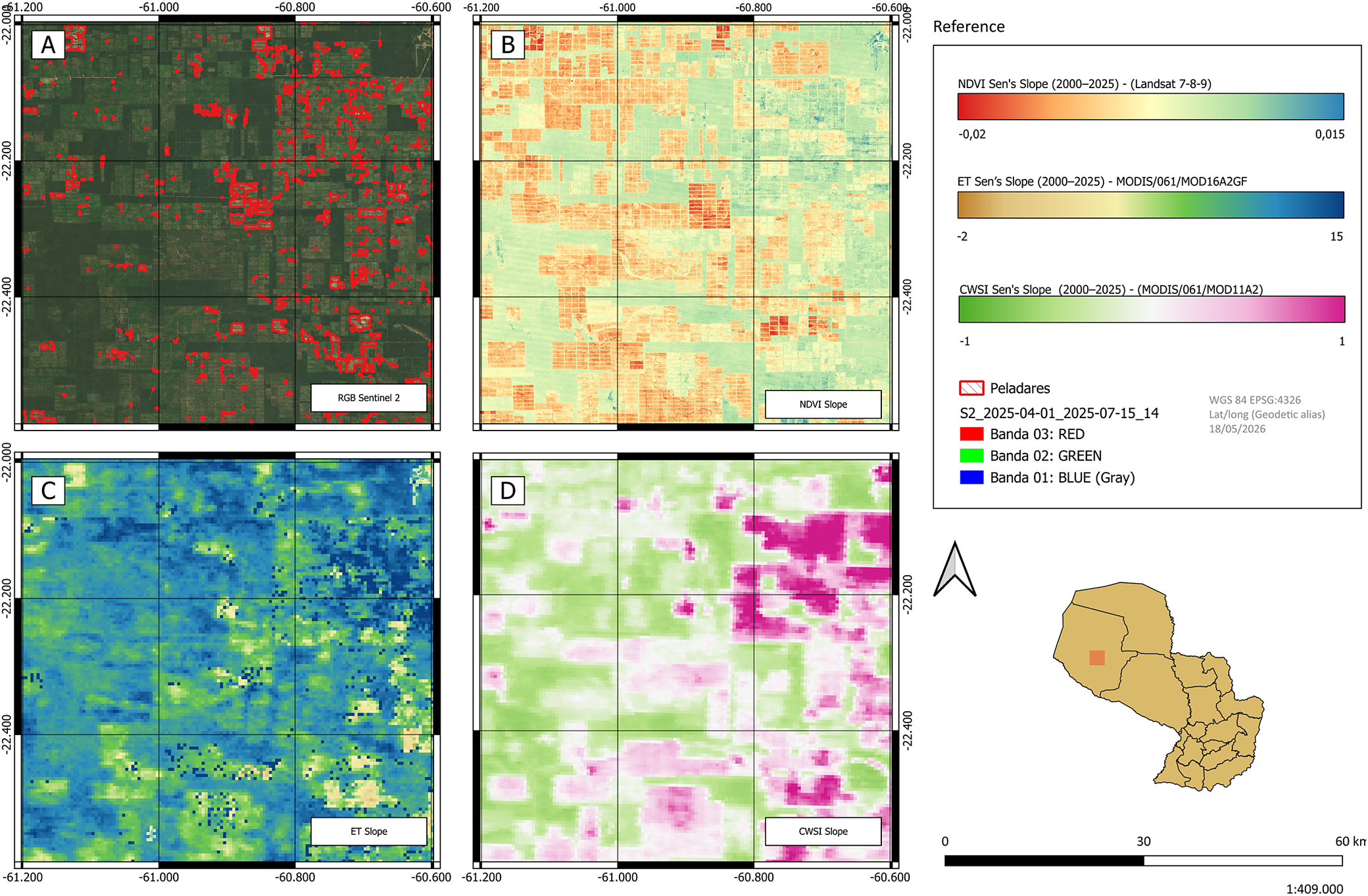
Optical satellite image of the study area showing the location of peladares, red polygons (a) and spatial patterns of NDVI (b), ET (c) and CWSI (d) slopes.

Figure 2. Long description
A multi-panel set of geographical maps labeled A through D, each showing the same gridded region between latitudes -22.000 and -24.400 and longitudes -61.200 and -60.600.
* Panel A, top-left, is an R G B Sentinel 2 satellite photo showing dark green forested areas interspersed with red polygons representing peladares.
* Panel B, top-right, displays N D V I Sen’s Slope from 2000 to 2025. The color scale ranges from orange negative 0.02 to teal 0.015, showing a mix of stable and slightly declining vegetation health.
* Panel C, bottom-left, displays E T Sen’s Slope from 2000 to 2025. The color scale ranges from brown negative 2 to dark blue 15, indicating evapotranspiration trends.
* Panel D, bottom-right, displays C W S I Sen’s Slope from 2000 to 2025. The color scale ranges from green negative 1 to magenta 1, showing crop water stress index trends with a high concentration of magenta in the East.
A Reference box on the right contains the three color scales and a legend for the peladares red outline. Below the reference is a North arrow and a locator map of Paraguay with a red square highlighting the study area in the Northwest. A scale bar at the bottom indicates 0 to 60 kilometers.
Remote sensing-based monitoring of pasture degradation in the Paraguayan Chaco
Remote sensing technology is a valuable tool for mapping pasture degradation, especially at regional scales. One key example is the FAO’s global assessment of land degradation and improvement (GLADA), which used NDVI data, a parameter frequently used to evaluate vegetation health and productivity, from 1981 to 2003 to identify degradation trends. GLADA’s report showed that around 20% of the global land area, representing 2.7 billion ha, is degraded (Bai et al., Reference Bai, Dent, Olsson and Schaepman2008).
In the Paraguayan Chaco, livestock production depends almost exclusively on extensive pastures dominated by Gatton panic (MAG, 2023). Grassland ecosystems allocate ~60% of net primary productivity belowground, promoting soil organic carbon (SOC) accumulation under nondegraded and well-managed conditions (Jackson et al., Reference Jackson, Lajtha, Crow, Hugelius, Kramer and Piñeiro2017). Evidence from South American biomes indicates that improved pasture management can increase SOC stocks by 7–20% compared to native vegetation and substantially enhance carbon sequestration through optimized grazing practices (Maia et al., Reference Maia, Ogle, Cerri and Cerri2009; Fujisaki et al., Reference Fujisaki, Perrin, Desjardins, Bernoux, Balbino and Brossard2015; de Oliveira et al., Reference Oliveira, Silva, Baumann, Miziara, Ferreira and Merelles2022; Bai and Cotrufo, Reference Bai and Cotrufo2022; Ribeiro et al., Reference Ribeiro, Maculan, de Ávila, Morais, Hoeckesfeld, Secchi and de Andrade Guerra2025). In contrast, pasture degradation leads to SOC losses ranging from 10% to 56% and is widespread across major cattle-producing regions, including the Brazilian Cerrado, where nearly half of the pastures are degraded (Guareschi et al., Reference Guareschi, Pereira and Perin2013; de OliveiraSilva et al., Reference de Oliveira, Barioni, Hall, Folegatti Matsuura, Zanett Albertini, Fernandes and Morgan2016; Medeiros et al., Reference Medeiros, Maia, Santos and Gomes2020; Pereira et al., Reference Pereira, Ferreira, Pinto and Baumgarten2018). Despite its importance, the extent of pasture degradation in the Paraguayan Chaco, home to 44% of the national livestock herd, remains undocumented, highlighting the need for systematic mapping and monitoring to support sustainable grazing management and evidence-based policy development (MAG, 2023).
To establish the first comprehensive record on pasture degradation in the study region, we evaluated annual NDVI (Normalized Difference Vegetation Index)-time series data following the conversion of native forest to pasture or crops. NDVI was used as a proxy to assess degradation trends, following the approach described by Pereira et al. (Reference Pereira, Ferreira, Pinto and Baumgarten2018). To evaluate vegetation condition within the selected region, NDVI slope values were spatially intersected with the classified land-cover categories. This integration enabled the quantification and mapping of long-term NDVI decline in pasture-dominated areas, allowing the identification of zones exhibiting early signs of degradation (Figure 2b).
We noticed a negative NDVI trend across substantial portions of the rangeland situated in the study area (Figure 2b). On the other hand, the central region of the Paraguayan Chaco, where intensive agricultural activities take place, exhibited a near-neutral to positive NDVI trend over the 2000–2024 period (Henderson et al., Reference Henderson, Godar, Frey, Börner and Gardner2021; Supplementary Figure 2a). These opposing NDVI trends likely reflect a redistribution of land-use intensity, with livestock production increasingly expanding into rangeland areas more prone to degradation. Altogether, this dataset provides a foundation for identifying the drivers of pasture degradation under ongoing climate change and elevated deforestation rates, and for informing strategies to restore degraded areas.
Consequently, the relationship between year of deforestation (2000–2024) and NDVI slope was strongly nonlinear (Supplementary Figure 3a). NDVI trends were most negative in areas deforested during intermediate periods, indicating intensified pasture degradation following land conversion. In contrast, older deforested areas exhibited less negative or near-stable trends, suggesting apparent stabilization. This pattern should not be interpreted as ecological recovery, but instead reflects spatial heterogeneity in land suitability and frontier expansion dynamics, whereby early deforestation preferentially targeted more productive landscapes, while subsequent clearing progressively expanded into more marginal areas. Notably, areas deforested most recently (2021–2024) exhibited NDVI slopes closer to zero than those cleared between 2010 and 2020, consistent with limited time since conversion and the persistence of residual soil fertility, organic matter and soil moisture following clearing. Apparent stabilization in older areas may also arise from pasture abandonment, secondary vegetation regrowth, woody encroachment or long-term mismanagement, whereby increases or stabilization in NDVI reflect changes in vegetation structure rather than improvements in pasture condition.
MODIS-derived crop water stress index for monitoring drought throughout prolonged time periods
Paraguay has a significant portion of its land categorized as drylands, around 53%, which are exceptionally vulnerable to anthropogenic climate and land-use change, with increasing risk of desertification (Burrell et al., Reference Burrell, Evans and De Kauwe2020; Ganem et al., Reference Ganem, Xue, Rodrigues, Franca-Rocha, Oliveira, Carvalho, Turpo Cayo, Rosa, Dutra and Shimabukuro2022). The current climatic scenario, marked by increasing drought severity and rising temperature, along with declining annual precipitation, is causing a substantial decline in land productivity in these fragile ecosystems, threatening plant diversity that sustains carbon storage and nutrient cycling (Maestre et al., Reference Maestre, Quero, Gotelli, Escudero, Ochoa, Delgado- Baquerizo, Garcia-Gomez, Bowker, Soliveres, Escolar, Garcia-Palacios, Berdugo, Valencia, Gozalo, Gallardo, Aguilera, Arredondo, Blones, Boeken, Bran, Conceicao, Cabrera, Chaieb, Derak, Eldridge, Espinosa, Florentino, Gaitan, Gatica, Ghiloufi, Gomez-Gonzalez, Gutierrez, Hernandez, Huang, Huber-Sanwald, Jankju, Miriti, Monerris, Mau, Morici, Naseri, Ospina, Polo, Prina, Pucheta, Ramirez-Collantes, Romao, Tighe, Torres-Diaz, Val, Veiga, Wang and Zaady2012; Ganem et al., Reference Ganem, Xue, Rodrigues, Franca-Rocha, Oliveira, Carvalho, Turpo Cayo, Rosa, Dutra and Shimabukuro2022).
In Chaco, annual rainfall is highly variable, marked with long periods of drought, and has a latitudinal gradient, decreasing from the southeast to northwest, while mean annual temperature increases from south to north (Houspanossian et al., Reference Houspanossian, Giménez, Baldi and Nosetto2016; Ruiz-Díaz et al., Reference Ruiz-Díaz, de Molas, Benítez-León, Zambrano, Johnson, Bohlman and Broadbent2024). Across much of the northwestern region of the Paraguayan dry Chaco, rainfall inputs (500–700 mm annually) are surpassed by evapotranspiration (ET), preventing deep drainage and salt leaching (Ruiz-Díaz et al., Reference Ruiz-Díaz, de Molas, Benítez-León, Zambrano, Johnson, Bohlman and Broadbent2024) (Figure 2c). In Supplementary Figure 2b, the impact of land-use change on the ET rate is shown, highlighting its reduction afterward conversion to crops or pasture, which triggers deep drainage and groundwater recharge. This land-use change-hydrology interaction sets secondary salinization onset and therefore should be regularly monitored in order to determine the extent of salinization progress and areas that are prone to salinization. In addition, ET exhibited a nonlinear relationship with deforestation timing, with the highest ET observed in recently deforested areas (post-2020) and a minimum in areas cleared between 2010 and 2015 (Supplementary Figure 3b). ET in older deforested areas increased relative to this minimum but remained lower than in recently cleared regions, likely reflecting environmental differences among deforestation cohorts rather than post-deforestation recovery.
Remote sensing enables continuous spatiotemporal monitoring of vegetation dynamics and drought conditions (Clark et al., Reference Clark, Aide, Grau and Riner2010). Among agricultural drought indicators, the Crop Water Stress Index (CWSI), derived from surface energy balance theory, is considered one of the most accurate metrics of plant water stress (Bai et al., Reference Bai, Yu and Di2017). CWSI quantifies stress as the normalized difference between actual canopy-air temperature and two reference baselines: a non-water-stressed baseline representing optimal transpiration and a maximum stress baseline representing fully inhibited transpiration, with values ranging from 0 (no stress) to 1 (maximum stress) (Tian et al., Reference Tian, Hou, Qiu, Zhang and Yuan2020; Liao et al., Reference Liao, Gu, Gao, Du, Kang, Tong and Ding2024). In this study, CWSI was calculated using land surface temperature from MOD11A2 daily data (2000–2024) following the method of Liao et al. (Reference Liao, Gu, Gao, Du, Kang, Tong and Ding2024), which accounts for key biophysical controls on water availability, such as soil water-holding capacity and crop type, that are closely linked to yield (Djebou et al., Reference Djebou, Singh and Frauenfeld2015) (Figure 2d).
Supplementary Figure 2c shows that, in the Paraguayan Chaco, CWSI is strongly related to land-use type and geographical location, as the southern region, where precipitation and water conservation ability are higher and temperature is lower, displayed values closer to zero. In contrast, the central and northern regions, specifically in areas where native dry woods were replaced by crops and pasture, reported higher CWSI values. This parameter, used to diagnose water and salt stress in plants, indicates that a significant portion of crops and pastures in this semi-arid region are severely affected by abiotic stresses such as drought and, potentially, salinization (Gu et al., Reference Gu, Liao, Gao, Kang and Ding2021; Bo et al., Reference Bo, Guan and Mao2023).
Moreover, the CWSI slope was estimated to evaluate variation in plant water relations following land-use change to pasture in the study area. The relationship between year of clearing and CWSI slope was strongly nonlinear (Supplementary Figure 3c). CWSI peaked in areas cleared between 2011 and 2015, indicating maximum disruption of evapotranspiration and elevated vegetation water stress following land-use change. Older cleared areas exhibited lower CWSI values, while more recently deforested areas (2021–2024) showed declining CWSI, likely reflecting short-term vegetation establishment and transitional land-cover conditions. These results suggest that CWSI captures cumulative land-use legacy effects rather than immediate disturbance, and that assessments focused solely on recent deforestation may underestimate longer-term degradation processes. Furthermore, a clear and nearly linear relationship was observed between vegetation degradation and water stress (Supplementary Figure 4), with increasingly negative NDVI slopes associated with higher CWSI values. This indicates a strong coupling between land degradation processes and plant water stress.
Overall, these patterns highlight the importance of incorporating time since clearing into remote sensing-based assessments of land degradation and water stress. They further underscore the need for climate-resilient crops and pastures, and adaptive grazing management strategies, such as stocking rate adjustment, supplementary forage, and deferred grazing during dry years, to sustain forage production and prevent further soil degradation under increasing climatic stress (Achon and Enciso Maldonado, Reference Achon and Enciso Maldonado2026).
Integrating multispectral classification and NDVI trends to track secondary salinization in semi-arid environments
Soil salinity differs from other stable soil properties in that it exhibits significant spatial variability and is highly dynamic. This variability makes determining the required number of samples to monitor this parameter a major challenge (Ma et al., Reference Ma, He, Ge and Luo2023). This characteristic of soil salinity also limits the ability to interpolate between ground measurements taken at individual points in space and time (Lobell et al., Reference Lobell2010). The spatial variability of soil salinity is influenced by soil factors (e.g., parent material, permeability, water table depth, groundwater electrical conductivity and topography), management factors (e.g., deforestation and irrigation) and climate factors (e.g., precipitation and evapotranspiration) (Allbed and Kumar, Reference Allbed and Kumar2013; Allbed et al., Reference Allbed, Kumar and Aldakheel2014).
Due to the significant lack of data quantifying the progression of salinization in the Dry Paraguayan Chaco, specifically field-collected data on soil electrical conductivity, water table electrical conductivity and the impacts of land-use changes on water table dynamics, a multi-indicator soil salinity monitoring model based on satellite remote sensing data and machine learning was employed.
It is important to note that conventional approaches to soil salinity measurement typically involve field soil sampling for laboratory analysis, followed by solute content determination, which are both time-consuming and costly (Hardie and Doyle, Reference Hardie, Doyle, Shabala and Cuin2012). Consequently, in recent years, the use of remote sensing techniques to assess soluble salt concentrations in soils has gained traction, as they offer extensive spatial–temporal monitoring capabilities. Several studies have demonstrated the validity of these remote sensing methods for studying the spatial distribution of saline soils. These techniques can be categorized into two types: direct assessments of bare soil and indirect assessments based on vegetation affected by soil salinity (Ma et al., Reference Ma, He, Ge and Luo2023).
Zhang et al. (Reference Zhang, Wu, Kang, Fan, Wang, Liu and He2024) developed a remote sensing and machine learning framework to estimate soil salinity by compiling and evaluating nine salinity indices derived from multispectral imagery and integrating topographic and climatic variables. They tested several machine learning algorithms, including Random Forest, to predict soil salinity across the landscape. These indices provide a robust basis for assessing salinity in other regions and were adopted in our study to evaluate potential soil salinization in the Boquerón region. Accordingly, we correlated all nine salinity indices with NDVI slope to assess whether higher salinity index values are associated with pasture degradation. Among them, the SI6 index exhibited the strongest association with pasture degradation, highlighting its potential as a candidate for validation through in situ soil sampling across different soil depths (Figure 3).
Salinity index ranking showing the relationship between SI values and NDVI-based pasture degradation.

Figure 3. Long description
The horizontal bar chart displays the absolute value of weighted r (N D V I _ resid, salinity) on the X-axis, ranging from 0.0 to 0.5. The Y-axis lists ten salinity indices. From top to bottom, the indices and their approximate correlation values are:
* S I 6: 0.52
* S I 9: 0.51
* S I 1: 0.50
* N D S I: 0.49
* S I 4: 0.48
* S I 3: 0.38
* S I 7: 0.33
* S I 5: 0.30
* S I 2: 0.23
* S I 8: 0.15
The chart shows a clear hierarchy where S I 6 has the strongest association with year-adjusted N D V I degradation, while S I 8 has the weakest.
Soil salinity is a major land degradation process that severely affects productivity and sustainability in semi-arid regions (Kılıc et al., Reference Kılıc, Budak, Gunal, Acır, Halbac-Cotoara-Zamfir, Alfarraj and Ansari2022). The literature identifies salinization as a key driver of pasture degradation in these environments, not only as a chemical stressor but also as a factor contributing to the decline of soil organic matter, a critical indicator of biological degradation. However, pasture degradation is a multifactorial process also influenced by overgrazing (resulting from inadequate management), declining soil fertility, soil erosion, the spread of invasive weeds, reduction of root systems and grass mortality, all of which reduce organic matter inputs into the soil. In addition, prolonged drought periods play a significant role in accelerating pasture degradation (Maia et al., Reference Maia, Carvalho, Cerri, Lal, Bernoux, Galdos and Cerri2013; Guareschi et al., Reference Guareschi, Pereira and Perin2013; de Oliveira Silva et al., Reference de Oliveira, Barioni, Hall, Folegatti Matsuura, Zanett Albertini, Fernandes and Morgan2016; Veldkamp et al., Reference Veldkamp, Schmidt, Powers and Corre2020; Bolfe et al., Reference Bolfe, Victoria, Sano, Bayma, Massruhá and de Oliveira2024; Berdgett et al., Reference Berdgett, Bullock, Lavorel, Manning, Schaffner, Ostle, Chomel, Durigan, Fry, Johnson, Lavallee, Le Provost, Lou, Png, Sankaran, Hou, Zhou, Ma, Ren, Li, Ding, Li and Shi2021).
Consistent with these processes, Supplementary Figure 4 shows a significant negative relationship between NDVI Sen’s slope and CWSI Sen’s slope (p < 0.001), indicating that areas experiencing stronger declines in vegetation greenness over time also tend to exhibit increasing water stress. This pattern is consistent across land-use cohorts, with more recently cleared areas generally showing steeper NDVI declines and greater increases in CWSI, suggesting more pronounced degradation dynamics. However, some of the most recently cleared areas still display neutral or even positive NDVI trends, possibly reflecting a temporal lag before the full effects of vegetation decline and water stress become evident. In contrast, older or stable non-forest areas exhibit weaker trends. Overall, these findings indicate that land-use change is associated with a coupled trajectory of declining vegetation and increasing water stress, supporting the interpretation that recently cleared areas are undergoing progressive degradation.
Satellite-derived indices capture variation associated with processes beyond direct climatic controls, potentially including soil properties and land-use dynamics. This is reflected in the relatively weak relationship between precipitation and vegetation dynamics. Over a 35-year period, the association between annual mean precipitation and annual mean NDVI (Supplementary Figure 5) indicates that precipitation explains <25% of the variability in NDVI in peladares areas, despite being highly statistically significant. In contrast, Supplementary Figure 4, which shows Sen’s slope trends for CWSI and NDVI, indicates that CWSI explains ~72% of the variability in NDVI.
These results suggest that vegetation dynamics are more strongly regulated by plant water stress than by precipitation alone, highlighting the importance of integrated indicators that account for both climatic and soil-vegetation interactions.
Exploring salinity management in the Paraguayan Chaco: A pipeline for studying impacts and developing sustainable solutions
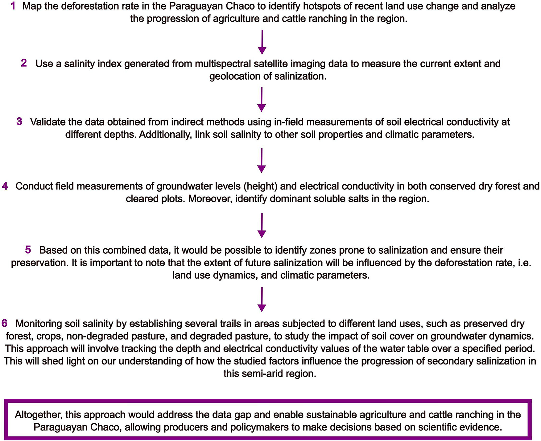
Significant data gaps persist regarding water table depth, soil properties and groundwater salinity across Paraguay, and the long time lag between deforestation-driven recharge increases and the manifestation of secondary salinization complicates early detection in drylands (Beresford et al., Reference Beresford, Phillips and Bekle2001). Because salinization develops belowground, systematic monitoring of groundwater depth and electrical conductivity, coupled with land-use change dynamics, is essential for anticipating salinity risks. Addressing this challenge requires regional-scale assessments across the dry-humid Chaco transition zone to capture spatial patterns, identify emerging hotspots and detect trends not evident at local scales (Shokri et al., Reference Shokri, Hassani and Sahimi2024). Integrating ecohydrological indicators, including soil characteristics, aridity indices and groundwater depth and salinity, into predictive mapping frameworks would enable the identification of areas most vulnerable to secondary salinization and support targeted management, policy development and sustainable land-use planning. Following this rationale, we propose a pipeline to systematically address secondary salinization in the Paraguayan Chaco, combining monitoring, predictive mapping and targeted management actions (Figure 4). In parallel, disseminating salinization risk maps could raise awareness of the threat posed to agricultural expansion, help curb deforestation, promote restoration practices and inform effective land management in the Chaco’s dry forests.
Proposed pipeline to assess secondary salinization progression in the Paraguayan Chaco.

Figure 4. Long description
The flowchart consists of six numbered steps connected by downward arrows, concluding with a summary box at the bottom.
* Step 1. Map the deforestation rate in the Paraguayan Chaco to identify hotspots of recent land use change and analyze the progression of agriculture and cattle ranching in the region.
* Step 2. Use a salinity index generated from multispectral satellite imaging data to measure the current extent and geolocation of salinization.
* Step 3. Validate the data obtained from indirect methods using in-field measurements of soil electrical conductivity at different depths. Additionally, link soil salinity to other soil properties and climatic parameters.
* Step 4. Conduct field measurements of groundwater levels height and electrical conductivity in both conserved dry forest and cleared plots. Moreover, identify dominant soluble salts in the region.
* Step 5. Based on this combined data, it would be possible to identify zones prone to salinization and ensure their preservation. It is important to note that the extent of future salinization will be influenced by the deforestation rate, i.e. land use dynamics, and climatic parameters.
* Step 6. Monitoring soil salinity by establishing several trails in areas subjected to different land uses, such as preserved dry forest, crops, non-degraded pasture, and degraded pasture, to study the impact of soil cover on groundwater dynamics. This approach will involve tracking the depth and electrical conductivity values of the water table over a specified period. This will shed light on our understanding of how the studied factors influence the progression of secondary salinization in this semi-arid region.
At the bottom, a purple-bordered box states: Altogether, this approach would address the data gap and enable sustainable agriculture and cattle ranching in the Paraguayan Chaco, allowing producers and policymakers to make decisions based on scientific evidence.
Conclusions
A key limitation of this study is the absence of direct in situ validation of the salinization patterns identified through remote sensing. The indicators used in this work rely on spectral responses and derived indices that act as proxies for soil salinity, and therefore reflect surface or near-surface conditions rather than direct measurements of soil electrical conductivity. As a result, the findings should be interpreted as relative indicators of salinization risk rather than absolute quantifications of soil salinity. Furthermore, without field-based calibration, uncertainties remain regarding the magnitude and depth of salinity processes. Despite these limitations, the spatial patterns identified are consistent with known environmental gradients and hydrological dynamics of the Dry Chaco, supporting the robustness of the observed trends.
The future extent of degradation in the Dry Chaco will depend on land-use dynamics, particularly the impact of anthropogenic change in areas prone to degradation, whether conserved or deforested. Hence, continuous monitoring of pasture degradation and the effects of abiotic stressors on livestock systems is essential, especially as the expansion of agriculture and rangeland activities increasingly encroaches into marginal areas more susceptible to degradation. Generating robust scientific evidence is crucial to inform sustainable management practices and to safeguard the ecological integrity of fragile dryland environments such as the Paraguayan Dry Chaco. In this context, this study provides a valuable basis for future research, particularly through the integration of systematic in situ validation of satellite-based multispectral approaches.
Open peer review
For open peer review materials, please visit https://doi.org/10.1017/dry.2026.10042.
Supplementary material
The supplementary material for this article can be found at http://doi.org/10.1017/dry.2026.10042.
Data availability statement
All data generated and analyzed in this study are included in the main text and Supplementary Figures.
Acknowledgments
The authors would like to acknowledge the “Consejo Nacional de Ciencia y Tecnología” (CONACYT) for financial support of this research.
Author contribution
E.A.C., G.A.E.M. and I.A. designed the study and conducted the analyses. All authors wrote and approved the manuscript.
Financial support
This work was supported by grants from the “Consejo Nacional de Ciencia y Tecnología” (PRIA01-17 and PRIA02-1 for Guillermo Enciso-Maldonado and Ignacio Achon).
Competing interests
The authors declare none.


 Open access


Comments
Prof. Osvaldo Sala and Prof. David Eldridge
Editors-in-Chief, Cambridge Prisms: Drylands
Cambridge University Press
Dear Professors Sala and Eldridge,
On behalf of my co-authors, I am pleased to submit the manuscript entitled “Assessing grassland degradation and potentially salt-affected soils in the Paraguayan Chaco using multispectral data” for consideration as a Research Article in Cambridge Prisms: Drylands.
Our study addresses an urgent drylands management challenge in the Paraguayan Chaco, where rapid forest conversion to extensive pastures is expanding into increasingly marginal environments and where field ecohydrological and salinity data remain scarce. Using a ~500,000 ha case study in Boquerón, we present a scalable workflow that integrates (i) object-based Random Forest mapping of bare-soil “peladares” from Sentinel-2 during peak greenness, (ii) two decades of trend analysis in vegetation condition, evapotranspiration, and thermal water-stress metrics (NDVI, ET, CWSI) using Sen’s slope, and (iii) a cohort-residualization approach to separate land-use history effects from within-cohort degradation signals. We then evaluate and rank multiple optical salinity indices, identifying SI6 as the most informative proxy for prioritizing sites for in situ validation and monitoring of secondary salinization risk.
We believe this contribution aligns well with the journal’s mission of publishing high-impact, transdisciplinary research that advances understanding and management of global drylands, and it offers a practical early-warning screening approach that can be transferred to other dryland frontiers facing similar pressures.
This manuscript is original, has not been published previously, and is not under consideration elsewhere. All authors have approved the submission. The authors declare no conflicts of interest. Funding support (CONACYT PRIA01-17 and PRIA02-1) and a data availability statement are included in the manuscript.
Corresponding authors:
Emilio Aguilar Cubilla (emilio.aguilarcubilla@gmail.com)
Ignacio Achon (ignacio.achon@agr.una.py)
Thank you for your time and consideration. We look forward to your response.
Sincerely,
Dr. Ignacio Achon (on behalf of all authors)