Introduction
The woolly mammoth (Mammuthus primigenius Blum.) is an iconic representative of the Late Pleistocene megafauna (e.g. Stuart Reference Stuart2021, 43–50). Its existence and extinction in Eurasia are relatively well-studied (Kuzmin Reference Kuzmin2010; Kuzmin and Orlova Reference Kuzmin and Orlova2004; MacDonald et al. Reference MacDonald, Beilman, Kuzmin, Orlova, Kremenetski, Shapiro, Wayne and Van Valkenburgh2012; Nikolskiy and Pitulko Reference Nikolskiy and Pitulko2013; Stuart et al. Reference Stuart, Sulerzhitsky, Orlova, Kuzmin and Lister2002). Nevertheless, several issues related to the spatiotemporal distribution of this species over the last 50,000 years are not very clear. One of the most important questions is this: what is the relationship between the climatic fluctuations in the second part of the Late Pleistocene and the patterns of existence for woolly mammoths? Also, the dynamics of the final disappearance for mammoths in the eastern part of Eurasia (i.e. Siberia) need to be clarified (see MacDonald et al. Reference MacDonald, Beilman, Kuzmin, Orlova, Kremenetski, Shapiro, Wayne and Van Valkenburgh2012; Nikolskiy and Pitulko Reference Nikolskiy and Pitulko2013; Orlova et al. Reference Orlova, Kuzmin, Zenin and Dement’ev2003; Pitulko and Nikolskiy Reference Pitulko and Nikolskiy2012; Puzachenko et al. Reference Puzachenko, Markova, Kosintsev, van Kolfschoten, van der Plicht, Kuznetsova, Tikhonov, Ponomarev, Kuitems and Bachura2017). Nowadays, this can be done by using the extensive radiocarbon (14C) databases and applying the Geographic Information System (GIS) software.
Therefore, the aim of this paper is twofold: 1) to present the updated spatiotemporal patterns of existence and extinction of mammoth in Siberia based on its 14C-dated remains; and 2) to compare the dynamics of mammoth populations and climatic changes over the last 50,000 years.
Material and methods
Our updated database for mammoths in Siberia (see Arppe et al. Reference Arppe, Karhu, Vartanyan, Drucker, Etu-Sihvola and Bocherens2019; Dehasque et al. Reference Dehasque, Pečnerová, Muller, Tikhonov, Nikolskiy, Tsigankova, Danilov, Díez-del-Molino, Vartanyan, Dalén and Lister2021, Reference Dehasque, Morales, Díez-del-Molino, Pečnerová, Chacón-Duque, Kanellidou, Muller, Plotnikov, Protopopov, Tikhonov, Nikolskiy, Danilov, Giannì, van der Sluis, Higham, Heintzman, Oskolkov, Gilbert, Götherström, van der Valk, Vartanyan and Dalén2024; Kuzmin and Orlova Reference Kuzmin and Orlova2004; Kuzmin et al. Reference Kuzmin, Leshchinskiy, Zenin, Burkanova, Zazovskaya and Samandrosova2024; Kuitems et al. Reference Kuitems, van Kolfschoten, Tikhonov and van der Plicht2019; MacDonald et al. Reference MacDonald, Beilman, Kuzmin, Orlova, Kremenetski, Shapiro, Wayne and Van Valkenburgh2012; Nikolskiy et al. Reference Nikolskiy, Basilyan, Sulerzhitsky and Pitulko2010, Reference Nikolskiy, Sulerzhitsky and Pitulko2011; Palkopoulou et al. Reference Palkopoulou, Mallick, Skoglund, Enk, Rohland, Li, Omrak, Vartanyan, Poinar, Götherström, Reich and Dalén2015) contains ca. 970 14C values obtained from bones, teeth, and tusks (Supplement, Table S1). The codes for Russian laboratories are available in Kuzmin et al. (Reference Kuzmin, Burova, Zazovskaya, Zaretskaya, Savinetsky and Khasanov2022, 590–591). Dates with large standard deviations, greater than ca. 1500 14C years, were excluded. These values have very large calendar age intervals, and this can distort the dataset. Also, the number of these dates is not large, no more than 40–50. The ca. 115 “infinite” 14C values (i.e. greater than ca. 50,000 BP) were not included because it is impossible to calibrate them with necessary precision. In order to normalize selected dates, 1000-year intervals were chosen to combine the raw 14C dates into “occupation episodes” sensu Kuzmin and Keates (Reference Kuzmin and Keates2005) and Fiedel and Kuzmin (Reference Fiedel and Kuzmin2007). As a result, 618 “occupation episodes” (hereafter, episodes) were counted (Supplement, Table S2). This dataset is the basis for our further analysis.
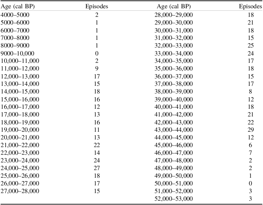
In order to combine 970 14C dates into 618 episodes, the following steps were undertaken. We combined into a single “occupation episode” all 14C dates from the same locality which belong to the 1000-year interval. For example, 165 Holocene 14C values (ca. 3685–8900 BP) for the Wrangel Island (Supplement, Table S1) were combined to five calendar intervals (using the youngest 14C dates which were calibrated, and the mean calendar age was calculated) (Table 1): 4000–5000 cal BP: 2 episodes; 5000–6000 cal BP – 1 episode; 6000–7000 cal BP – 1 episode; and 7000–8000 cal BP – 1 episode. After combining 14C-dated localities into 1000-year intervals, the frequencies for all intervals, from 4000–5000 cal BP to 52,000–53,000 cal BP, were calculated (Table 1). For calibration of 14C dates, the Calib Rev 8.1.0 software was used (see http://calib.org/calib/download/), in connection with the IntCal20 calibration curve (Reimer et al. Reference Reimer, Austin, Bard, Bayliss, Blackwell, Bronk Ramsey, Butzin, Cheng, Edwards, Friedrich, Grootes, Guilderson, Hajdas, Heaton, Hogg, Hughen, Kromer, Manning, Muscheler, Palmer, Pearson, van der Plicht, Reimer, Richards, Scott, Southon, Turney, Wacker, Adolphi, Büntgen, Capano, Fahrni, Fogtmann-Schulz, Friedrich, Köhler, Kudsk, Miyake, Olsen, Reinig, Sakamoto, Sookdeo and Talamo2020). Mean values for calibrated ranges were calculated and used (Table 2; Supplement, Table S2).
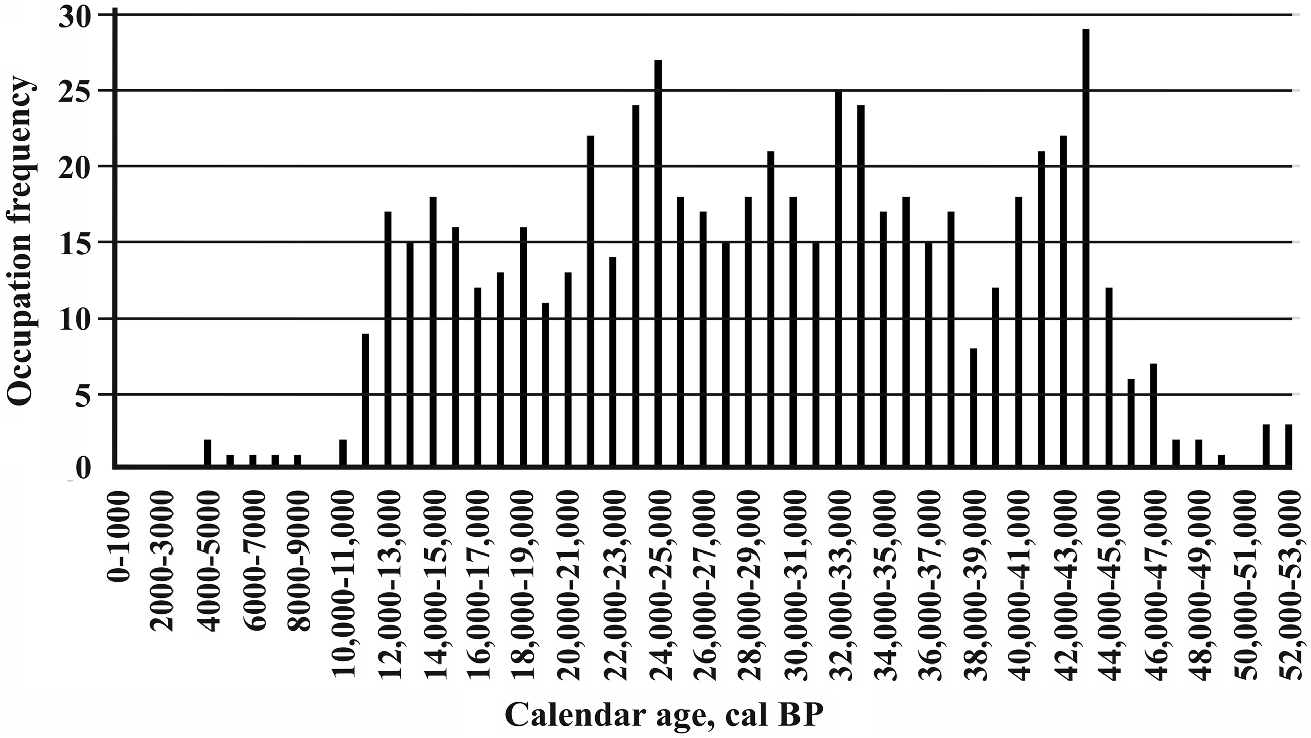
Frequencies of occupation episodes (calibrated, cal BP) for mammoths in Siberia (see Figure 2)

Table 1 Long description
A table showing frequencies of occupation episodes for mammoths in Siberia over different time periods. The table has two main sections, each with 28 rows and 2 columns. The first section lists age ranges in calibrated years before present (cal BP) and the corresponding number of episodes. The second section lists specific age ranges in calibrated years before present (cal BP) and the corresponding number of episodes. The table captures the frequencies of occupation episodes for mammoths in Siberia from 4000-5000 cal BP to 52000-53000 cal BP. Row 1: Age (cal BP), 4000-5000; Episodes, 2. Row 2: Age (cal BP), 5000-6000; Episodes, 1. Row 3: Age (cal BP), 6000-7000; Episodes, 1. Row 4: Age (cal BP), 7000-8000; Episodes, 1. Row 5: Age (cal BP), 8000-9000; Episodes, 1. Row 6: Age (cal BP), 9000-10000; Episodes, 0. Row 7: Age (cal BP), 10000-11000; Episodes, 2. Row 8: Age (cal BP), 11000-12000; Episodes, 9. Row 9: Age (cal BP), 12000-13000; Episodes, 17. Row 10: Age (cal BP), 13000-14000; Episodes, 15. Row 11: Age (cal BP), 14000-15000; Episodes, 18. Row 12: Age (cal BP), 15000-16000; Episodes, 16. Row 13: Age (cal BP), 16000-17000; Episodes, 12. Row 14: Age (cal BP), 17000-18000; Episodes, 13. Row 15: Age (cal BP), 18000-19000; Episodes, 16. Row 16: Age (cal BP), 19000-20000; Episodes, 11. Row 17: Age (cal BP), 20000-21000; Episodes, 13. Row 18: Age (cal BP), 21000-22000; Episodes, 22. Row 19: Age (cal BP), 22000-23000; Episodes, 14. Row 20: Age (cal BP), 23000-24000; Episodes, 24. Row 21: Age (cal BP), 24000-25000; Episodes, 27. Row 22: Age (cal BP), 25000-26000; Episodes, 18. Row 23: Age (cal BP), 26000-27000; Episodes, 17. Row 24: Age (cal BP), 27000-28000; Episodes, 15. Row 25: Age (cal BP), 28000-29000; Episodes, 18. Row 26: Age (cal BP), 29000-30000; Episodes, 21. Row 27: Age (cal BP), 30000-31000; Episodes, 18. Row 28: Age (cal BP), 31000-32000; Episodes, 15. Row 29: Age (cal BP), 32000-33000; Episodes, 25. Row 30: Age (cal BP), 33000-34000; Episodes, 24. Row 31: Age (cal BP), 34000-35000; Episodes, 17. Row 32: Age (cal BP), 35000-36000; Episodes, 18. Row 33: Age (cal BP), 36000-37000; Episodes, 15. Row 34: Age (cal BP), 37000-38000; Episodes, 17. Row 35: Age (cal BP), 38000-39000; Episodes, 8. Row 36: Age (cal BP), 39000-40000; Episodes, 12. Row 37: Age (cal BP), 40000-41000; Episodes, 18. Row 38: Age (cal BP), 41000-42000; Episodes, 21. Row 39: Age (cal BP), 42000-43000; Episodes, 22. Row 40: Age (cal BP), 43000-44000; Episodes, 29. Row 41: Age (cal BP), 44000-45000; Episodes, 12. Row 42: Age (cal BP), 45000-46000; Episodes, 6. Row 43: Age (cal BP), 46000-47000; Episodes, 7. Row 44: Age (cal BP), 47000-48000; Episodes, 2. Row 45: Age (cal BP), 48000-49000; Episodes, 2. Row 46: Age (cal BP), 49000-50000; Episodes, 1. Row 47: Age (cal BP), 50000-51000; Episodes, 0. Row 48: Age (cal BP), 51000-52000; Episodes, 3. Row 49: Age (cal BP), 52000-53000; Episodes, 3.
Relationships between AARs, occupation episodes, and δ18 O values (see Figure 4)

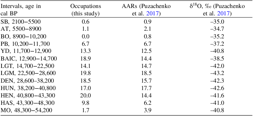
Table 2 Long description
A table with 12 rows and 4 columns comparing age intervals, occupations, AARs, and δ18O values. The columns are labeled 'Intervals, age in cal BP', 'Occupations (this study)', 'AARs (Puzachenko et al. 2017)', and 'δ18O, ‰ (Puzachenko et al. 2017)'. The rows are labeled with specific age intervals and corresponding values for occupations, AARs, and δ18O. Row 1: SB, 2100–5500, 0.6, 0.9, -35.0. Row 2: AT, 5500–8900, 1.1, 2.1, -34.7. Row 3: BO, 8900–10200, 0.0, 0.8, -35.2. Row 4: PB, 10200–11700, 6.7, 6.7, -37.2. Row 5: YD, 11700–12900, 13.3, 12.5, -40.8. Row 6: BAIC, 12900–14700, 18.9, 14.4, -38.5. Row 7: LGT, 14700–22500, 14.1, 14.7, -42.0. Row 8: LGM, 22500–28600, 19.8, 18.5, -43.2. Row 9: DEN, 28600–38200, 18.5, 15.7, -42.3. Row 10: HUN, 38200–40800, 17.0, 17.7, -42.6. Row 11: HEN, 40800–43300, 20.0, 14.4, -41.6. Row 12: HAS, 43300–48300, 9.8, 6.2, -41.0. Row 13: MO, 48300–54200, 1.7, 3.9, -40.8.
We compared our episodes with average accumulation rates (AARs) in Puzachenko et al. (Reference Puzachenko, Markova, Kosintsev, van Kolfschoten, van der Plicht, Kuznetsova, Tikhonov, Ponomarev, Kuitems and Bachura2017). The AARs are the estimates of the amount of 14C-dated localities with mammoth finds divided by the duration of each climatic-stratigraphic units (see Puzachenko et al. Reference Puzachenko, Markova, Kosintsev, van Kolfschoten, van der Plicht, Kuznetsova, Tikhonov, Ponomarev, Kuitems and Bachura2017; Supplement, Table S1) for Western and Eastern Siberia, and Southern Siberia and Northern China. This way the number of AARs for 1000 years in each unit was calculated (see Puzachenko et al. Reference Puzachenko, Markova, Kosintsev, van Kolfschoten, van der Plicht, Kuznetsova, Tikhonov, Ponomarev, Kuitems and Bachura2017, 72–73).
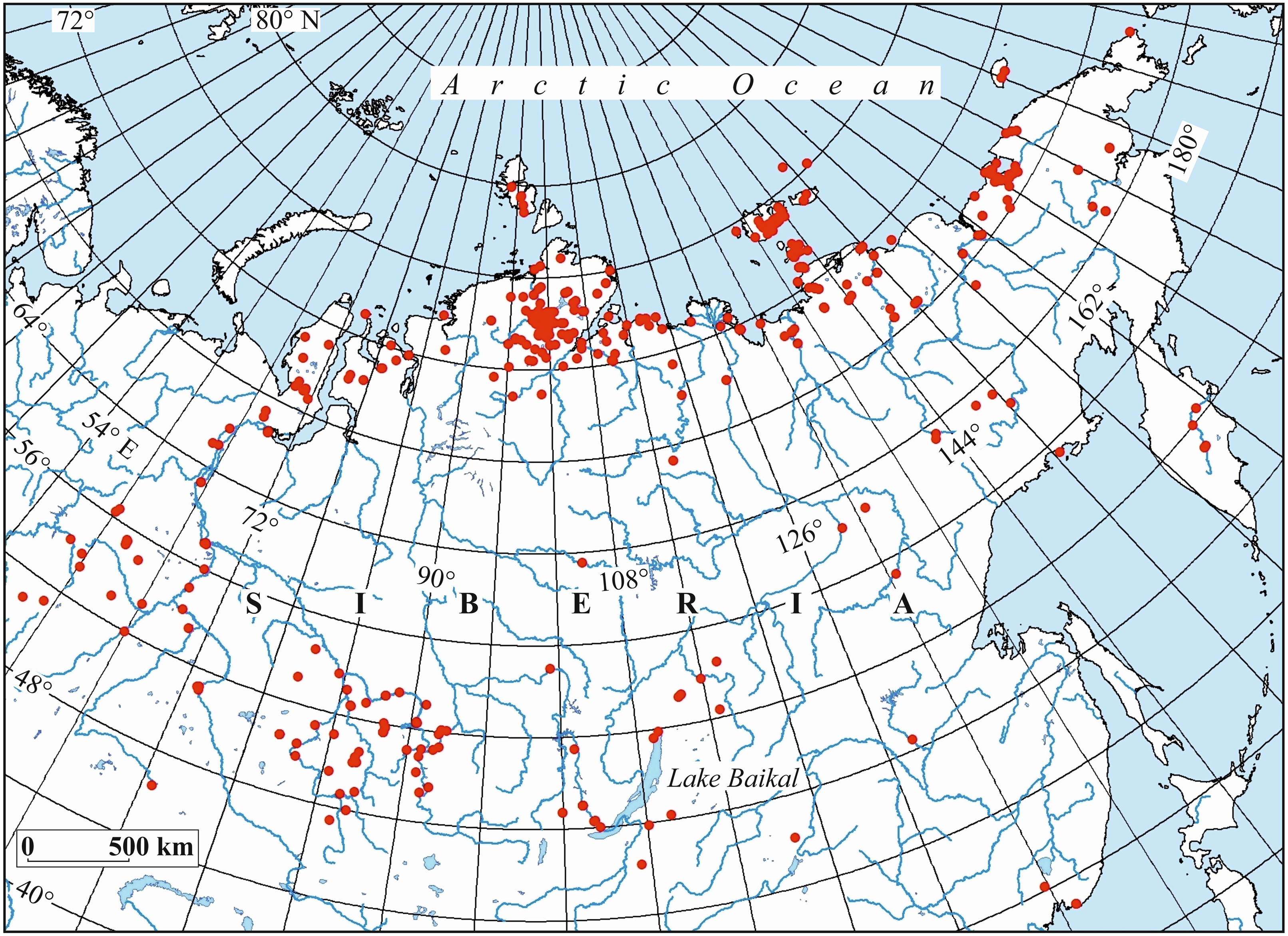
The spatial distribution of episodes in Siberia used in this study is presented in Figure 1. The density of them is not even, and the largest share of episodes (458, or ca. 74 % of the total number) is located in the north, above the 64°N (Supplement, Figure S1). This is due to the abundance of mammoth bones and tusks in the Siberian Arctic and sub-Arctic where it is easier to find them compared to the forested regions of Siberia south of ca. 64°N. To some extent, the large number of 14C dates and episodes for the Arctic part of Siberia is due to the long-term focus—since the 1960s—on collecting and 14C dating of mammoths in these regions (see Kuzmin and Orlova Reference Kuzmin and Orlova2004; Nikolskiy and Pitulko Reference Nikolskiy and Pitulko2013). Using the dataset of 618 episodes for the time interval of ca. 3600–51,000 BP, a diagram (Figure 2) and several distribution maps (Supplement, Figures S2–S12) were generated using the Geographic Information System software and analyzed. The spatial distribution of mammoth locations was visualized using the ArcGIS software package. A vector map of the world at a scale of 1:1,000,000 was used as the geographic basis.
Distribution of occupation episodes (each is represented by a 14C-dated case, see Table S2) for the woolly mammoth in Siberia.

Figure 1 Long description
A map showing the distribution of woolly mammoth occupation episodes in Siberia. The map covers a large portion of northern Eurasia, including Siberia and parts of Eastern Europe and the Arctic Ocean. Red dots are used to mark the locations of occupation episodes, each represented by a radiocarbon (14C) dated case. The map includes geographic features such as rivers, lakes, and major bodies of water like Lake Baikal. The red dots are scattered across the map, indicating the presence of woolly mammoths in various regions of Siberia. The map also includes latitude and longitude lines to provide a geographic reference. The purpose of the map is to illustrate the spatiotemporal distribution of woolly mammoths over the last 50,000 years and to clarify the dynamics of their final disappearance in the eastern part of Eurasia.
Diagram of the frequencies of calibrated occupation episodes (in cal BP) by 1000-years increments for the last ca. 53,000 years.

It is widely accepted that the number of 14C dates for certain objects (mainly finds of animal fossils and archaeological sites) reflects the size of population, although with some reservations (e.g. Bocquet-Appel et al. Reference Bocquet-Appel, Naji, Linden and Kozlowski2012; MacDonald et al. Reference MacDonald, Beilman, Kuzmin, Orlova, Kremenetski, Shapiro, Wayne and Van Valkenburgh2012; Nikolskiy et al. Reference Nikolskiy, Sulerzhitsky and Pitulko2011; Ugan and Byers Reference Ugan and Byers2008; Williams Reference Williams2012). One of the latest reviews of this approach can be found in Hoebe et al. (Reference Hoebe, Peeters and Arnoldussen2023).
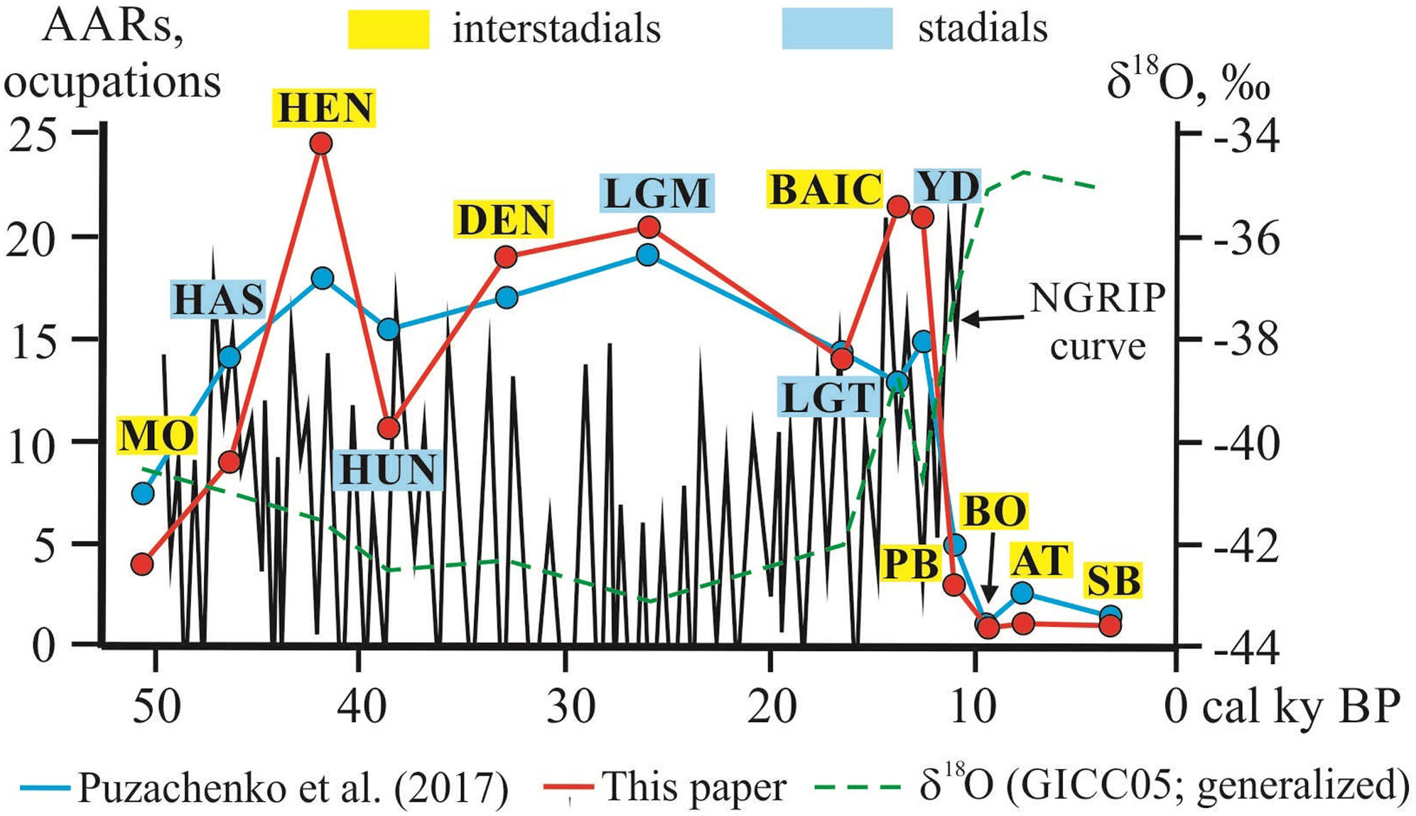
In order to compare the number of episodes and climatic changes in the last ca. 50,000 14C years, we used the approach initially employed by Puzachenko et al. (Reference Puzachenko, Markova, Kosintsev, van Kolfschoten, van der Plicht, Kuznetsova, Tikhonov, Ponomarev, Kuitems and Bachura2017). The number of 14C-dated mammoths were calculated for major climatic events, warm (i.e. interstadials) and cold (i.e. stadials): Moershoofd Interstadial (MO; ca. 48,300–54,200 cal BP; corresponds to Greenland events GI 13–14), Hasselo Stadial (HAS; ca. 43,300–48,300 cal BP; GS 12–13), Hengelo Interstadial (HEN; ca. 40,800–43,300 cal BP; GI 10–11), Huneborg Stadial (HUN; ca. 38,200–40,800 cal BP; GS 9–10), Denekamp Interstadial (DEN; ca. 28,600–38,200 cal BP; GI 4–8), Last Glacial Maximum Stadial (LGM; ca. 22,500–28,600 cal BP; GS 2.1–4), Late Glacial Transition (or Deglaciation) Stadial (LGT; ca. 14,700–22,500 cal BP; GS 2.1), Bølling–Allerød Interstadial (BAIC; ca. 12,900–14,700 cal BP; GI 1), Younger Dryas Stadial (YD; ca. 11,700–12,900 cal BP; GS 1); and Preboreal (PB; ca. 10,200–11,700 cal BP), Boreal (BO; ca. 8900–10,200 cal BP), Atlantic (AT; ca. 5500–8900 cal BP), and Subboreal (SB; ca. 2100–5500 cal BP) interstadials. These climate events are essentially of global or sub-global scale, and it seems appropriate to use it here.
The correlation with Greenland ice core warm (GI) and cold (GS) stages was done with the help of Rassmussen et al. (Reference Rasmussen, Bigler, Blockley, Blunier, Buchardt, Clausen, Cvijanovic, Dahl-Jensen, Johnsen, Fischer, Gkinis, Guillevic, Hoek, Lowe, Pedro, Popp, Seierstad, Steffensen, Svensson, Vallelonga, Vinther, Walker, Wheatley and Winstrup2014). The numbers for each interstadial/stadial were normalized for 1000 14C years due to the different durations of these climatic events. Numbers of AARs and occupation episodes were placed in the middle of these climatic events (see Results and Discussion), following Puzachenko et al. (Reference Puzachenko, Markova, Kosintsev, van Kolfschoten, van der Plicht, Kuznetsova, Tikhonov, Ponomarev, Kuitems and Bachura2017). We used simplified version of the δ18O curve (“average values of oxygen-isotope concentration”, see Puzachenko et al. Reference Puzachenko, Markova, Kosintsev, van Kolfschoten, van der Plicht, Kuznetsova, Tikhonov, Ponomarev, Kuitems and Bachura2017, 75, Fig. 2, caption).
Results and discussion
The variations in the number of calibrated 14C dates on Siberian mammoths through time are shown in Figure 2 (see also Table 1). The frequencies do not reveal any clear trend, with minima of 0–3 at ca. 47,000–50,000 cal BP and 0–2 at ca. 4000–10,000 cal BP, and maxima of 24–29 at ca. 23,000–25,000 cal BP, ca. 32,000–34,000 cal BP, and ca. 43,000–44,000 cal BP.
The spatiotemporal distribution of Siberian 14C-dated mammoths shows the following features (Supplement, Figures S2–S12). Until ca. 12,000 BP, mammoths inhabited all of Siberia, both southern and northern parts. Even during the LGM, ca. 19,000–23,000 BP, they did not disappear from the region (Figure S7), including its northern part (Figure S13). Since ca. 12,000 BP, the mammoth habitat began to shrink (Figures S9–S12). At ca. 10,600–12,000 BP, a few refugia south of 60° N still existed. An especially clear example is the Volchia Griva site in central Western Siberia (ca. 55° N) (see Figure S10), where mammoths survived until ca. 10,600–11,100 BP (Kuzmin et al. Reference Kuzmin, Leshchinskiy, Zenin, Burkanova, Zazovskaya and Samandrosova2024). After ca. 10,600 BP, 14C-dated mammoth finds are known only in the High Arctic (Figures S10–S12).
In today’s mainland Siberia (including the New Siberian Islands which were part of it until inundation of the surrounding space in the mid-Holocene by the rising Arctic Ocean level), the youngest 14C value is ca. 9500 BP (Supplement, Table S1, date GIN-11874). Most probably, the cause of mammoths’ disappearance from the mainland of Siberia was climatic warming and the emergence of treeless boggy tundra in the north and forests in the south, creating unfavorable environment for these mega-herbivores.
As for Wrangel Island as the last “stronghold” of mammoths in Siberia and worldwide, it was intermittently occupied since ca. 38,000–40,000 BP. At ca. 12,000–9000 BP, there is a gap in the mammoth record (e.g. Vartanyan et al. Reference Vartanyan, Arslanov, Karhu, Possnert and Sulerzhitsky2008); they re-appeared at ca. 9000 BP and existed until ca. 3700 BP, being the youngest known mammoths on Earth. It was suggested that the Taimyr Peninsula—where we have continuous records of the presence of mammoths at ca. 9700–11,100 BP (see Figures S9–S11)—was a source of the re-colonization of Wrangel Island by mammoths after ca. 9000 BP (Pečnerová et al. Reference Pečnerová, Palkopoulou, Wheat, Skoglund, Vartanyan, Tikhonov, Nikolskiy, van der Plicht, Díez-del-Molino and Dalén2017).
The cause(s) of the final extinction of the Wrangel Island mammoths in the Late Holocene is (are) still unclear. The climate of Wrangel Island in the terminal Pleistocene – Middle Holocene was of a moderate type (Lozhkin et al. Reference Lozhkin, Anderson, Vartanyan, Brown, Belaya and Kotov2001). The landscapes before and after ca. 10,000 BP were dominated by tundra with dwarf willow shrubs. Modern climatic conditions appeared at ca. 9000–10,000 BP, without significant variations during the Holocene (Lozhkin et al. Reference Lozhkin, Anderson, Vartanyan, Brown, Belaya and Kotov2001). The stable isotope data for mammoth from Wrangel Island shows no significant changes in the Holocene compared to the Late Pleistocene (Arppe et al. Reference Arppe, Karhu, Vartanyan, Drucker, Etu-Sihvola and Bocherens2019, 9, Fig. 5). The DNA data for the ca. 4300 14C-year-old mammoth bone from Wrangel Island demonstrates that the last surviving woolly mammoth population was subject to reduced genetic diversity with signs of inbreeding (Dehasque et al. Reference Dehasque, Morales, Díez-del-Molino, Pečnerová, Chacón-Duque, Kanellidou, Muller, Plotnikov, Protopopov, Tikhonov, Nikolskiy, Danilov, Giannì, van der Sluis, Higham, Heintzman, Oskolkov, Gilbert, Götherström, van der Valk, Vartanyan and Dalén2024; Palkopoulou et al. Reference Palkopoulou, Mallick, Skoglund, Enk, Rohland, Li, Omrak, Vartanyan, Poinar, Götherström, Reich and Dalén2015).
One of the most contentious issues in studies of mammoth existence and extinction is the relationship with climate as one of the major causes of its disappearance (e.g. Stuart Reference Stuart2021, 232–235; see also: Barnosky et al. Reference Barnosky, Koch, Feranec, Wing and Shabel2004; Koch and Barnosky Reference Koch and Barnosky2006; MacDonald et al. Reference MacDonald, Beilman, Kuzmin, Orlova, Kremenetski, Shapiro, Wayne and Van Valkenburgh2012). Puzachenko et al. (Reference Puzachenko, Markova, Kosintsev, van Kolfschoten, van der Plicht, Kuznetsova, Tikhonov, Ponomarev, Kuitems and Bachura2017) analyzed the dynamics of mammoth populations throughout the second part of the Late Pleistocene by calculating the frequencies of dated finds and comparing them with climate changes. They used the AAR parameter to quantify the changes in the intensity of occupation. The main conclusions of Puzachenko et al. (Reference Puzachenko, Markova, Kosintsev, van Kolfschoten, van der Plicht, Kuznetsova, Tikhonov, Ponomarev, Kuitems and Bachura2017, 85) are 1) the size of mammoth populations increased during the stadials, and decreased during the interstadials, because the landscapes of tundra-steppe (a.k.a. “mammoth steppe”) and periglacial forest steppe, typical during the stadials, were favorable for mammoths; and 2) climate played the main role in the process of mammoths’ extinction.
We applied the approach comparable to AAR to our database that is more complete than the one used by Puzachenko et al. (Reference Puzachenko, Markova, Kosintsev, van Kolfschoten, van der Plicht, Kuznetsova, Tikhonov, Ponomarev, Kuitems and Bachura2017). Our results are to some extent similar to their conclusions (Figure 3), but there are differences, probably because our dataset contains more direct 14C dates for Siberia. The most pronounced deviations are for the HEN, HUN, BAIC, and YD intervals. There are neither clear increases of occupation episodes during the stadials nor drops in the interstadials. This feature can be also traced in dataset by Puzachenko et al. (Reference Puzachenko, Markova, Kosintsev, van Kolfschoten, van der Plicht, Kuznetsova, Tikhonov, Ponomarev, Kuitems and Bachura2017). For example, there are large AAR numbers for the HEN, DEN, and BAIC interstadials. On the other hand, the difference between cold and warm climatic intervals are less pronounces in terms of AARs (Figure 3, line “Puzachenko et al. Reference Puzachenko, Markova, Kosintsev, van Kolfschoten, van der Plicht, Kuznetsova, Tikhonov, Ponomarev, Kuitems and Bachura2017”) than for occupation episodes (Figure 3, line “This paper”).
Distribution of AARs and occupation episodes for major climatic events in the last 50,000 14C years on the background of generalized δ18O records (after Puzachenko et al. Reference Puzachenko, Markova, Kosintsev, van Kolfschoten, van der Plicht, Kuznetsova, Tikhonov, Ponomarev, Kuitems and Bachura2017, Rasmussen et al. Reference Rasmussen, Bigler, Blockley, Blunier, Buchardt, Clausen, Cvijanovic, Dahl-Jensen, Johnsen, Fischer, Gkinis, Guillevic, Hoek, Lowe, Pedro, Popp, Seierstad, Steffensen, Svensson, Vallelonga, Vinther, Walker, Wheatley and Winstrup2014; with additions and modifications). MO – Moershoofd; HAS – Hasselo; HEN – Hengelo; HUN – Huneborg; DEN – Denekamp; LGM – Last Glacial Maximum; LGT – Late Glacial Transition; BAIC – Bølling–Allerød; YD – Younger Dryas; PB – Preboreal; BO – Boreal; AT – Atlantic; SB – Subboreal. The NGRIP curve was smoothed using the high and low values in Rasmussen et al. (Reference Rasmussen, Bigler, Blockley, Blunier, Buchardt, Clausen, Cvijanovic, Dahl-Jensen, Johnsen, Fischer, Gkinis, Guillevic, Hoek, Lowe, Pedro, Popp, Seierstad, Steffensen, Svensson, Vallelonga, Vinther, Walker, Wheatley and Winstrup2014).

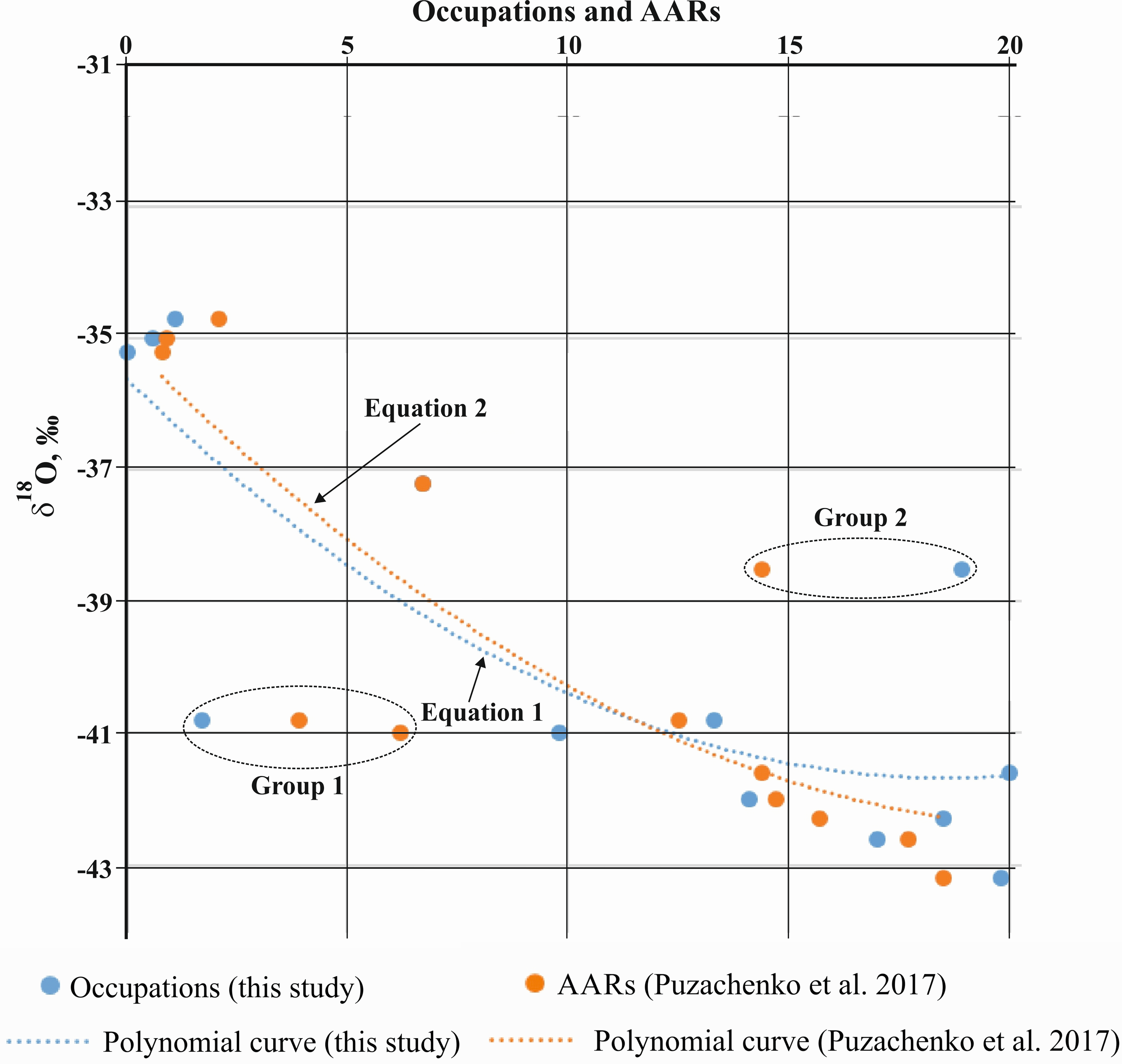
The relationship between the climate (expressed as generalized δ18O values from Greenland ice cores, see Table 2 and Figure 3), occupation episodes, and AARs was analyzed. Because the straightforward correlation is not clearly expressed, the trend analysis was applied. The resulting trend can be preliminary described as the decrease of δ18O along with increase of both episodes and AARs (Figure 4). It is expressed by the following equations of the polynomial curves of second order (Equation 1 is for data in this paper; and Equation 2 is for data of Puzachenko et al. Reference Puzachenko, Markova, Kosintsev, van Kolfschoten, van der Plicht, Kuznetsova, Tikhonov, Ponomarev, Kuitems and Bachura2017):
The trend curves of the climate (δ18O) vs. AARs and occupation episodes for mammoths in Siberia (see Table 2).

 $${\rm{y}} = 0.0177{{\rm{x}}^2}-0.6547{\rm{x}}-35.608{\rm{ }}\left( {{{\rm{r}}^2} = 0.6562} \right)$$
 $${\rm{y}} = 0.0156{{\rm{x}}^2}-0,6796{\rm{x}}-35.045\left( {{{\rm{r}}^2} = 0.7053} \right)$$
When one looks at the Figure 4 closely, two groups of dots (1 and 2) are visible. They seems to be the outliers of the trends expressed by curves. Group 1 (3 dots) centers around the δ18O value of –41‰; and Group 2 (2 dots) around δ18O value of –39‰. If we accept that the trends expressed by curves and equations 1–2 are correct, there are two anomalies of unclear nature. Also, there are other dots near the line of δ18O = –41‰, and their frequencies vary from ca. 2.0 to ca. 20.0. This clearly demonstrate the absence of direct correlation between climate, occupations, and AARs (Figure 4).
Both trends, based on our data and the results of work by Puzachenko et al. (Reference Puzachenko, Markova, Kosintsev, van Kolfschoten, van der Plicht, Kuznetsova, Tikhonov, Ponomarev, Kuitems and Bachura2017), are compatible (Figure 4), and most probably reflects the non-linear nature of the relationship between the climate and the size of mammoth populations for Siberia. Even though this is a preliminary conclusion (e.g. preliminary trend equations), it opens up the way for in-depth analysis of this phenomenon by using the modeling of parameters related to the size of mammoth population and climatic variables.
Due to long durations of climatic sub-divisions chosen by Puzachenko et al. (Reference Puzachenko, Markova, Kosintsev, van Kolfschoten, van der Plicht, Kuznetsova, Tikhonov, Ponomarev, Kuitems and Bachura2017) (MO, HAS, HEN, etc.), the direct comparison with the NGRIP dataset is impossible. It is clear that fixed 1000-year bins cannot properly represent the frequent rapid climate fluctuations as reflected in the NGRIP core (Rasmussen et al. Reference Rasmussen, Bigler, Blockley, Blunier, Buchardt, Clausen, Cvijanovic, Dahl-Jensen, Johnsen, Fischer, Gkinis, Guillevic, Hoek, Lowe, Pedro, Popp, Seierstad, Steffensen, Svensson, Vallelonga, Vinther, Walker, Wheatley and Winstrup2014). In the future, using other methods for comparison between mammoths and climate, like the Kernel Density Estimate (KDE) that does not use the fixed intervals for combining 14C dates, the result could be different. More work is still needed to test different approaches in numerical analysis of the 14C records.
Conclusions
The analysis of the updated 14C database of Siberian mammoths allows us to make the following conclusions. Up to ca. 12,000 BP, mammoths inhabited all the regions of Siberia. After that, the decreases in their numbers and size of habitat occurred, but until ca. 10,600 BP a few refugia existed south of 60°N. Since ca. 10,500 BP mammoths existed only in the High Arctic, north of ca. 68–70°N. The last population survived at ca. 9500–3700 BP on Wrangel Island. Before the final extinction, mammoths experienced a decrease in genetic diversity. The main factor for the disappearance of mammoth was most probably the climatic one.
The relationship between the dynamics of mammoth populations and climatic fluctuations (first of all, air temperature) in Siberia is non-linear. Generally, during interstadials the number of mammoths was larger than in the stadials; however, this trend is not straightforward. For example, a large frequency of mammoth 14C dates is detected for the cold Younger Dryas interval (ca. 12,500–10,500 BP). More work is needed to clarify this issue.
Supplementary material
To view supplementary material for this article, please visit https://doi.org/10.1017/RDC.2026.10197
Acknowledgments
A shorter version of this paper was delivered at the IVth International Conference “Radiocarbon in the Environment” (22–27 September 2024, University of Salento, Lecce, Italy). This study was supported by the State Assignment No. FWZN-2026-0004 of the Sobolev Institute of Geology and Mineralogy, Siberian Branch of the Russian Academy of Sciences, in Novosibirsk (Russia), with funds provided by the Ministry of Science and Higher Education of the Russian Deferation. We are grateful to Dr Susan G. Keates for polishing the grammar, and to two anonymous reviewers and Associate Editor of Radiocarbon Prof. Emeritus Peter Grootes for useful comments.