1 Introduction
The study of constructive and destructive interference of internal waves in non-uniform stratifications underlies our understanding of the passage of internal waves in the atmosphere and the ocean. In the atmosphere, winds blowing over topography can generate low-frequency internal waves widely known as lee waves (Bell Reference Bell1975; Baines & Hoinka Reference Baines and Hoinka1985). In the ocean, surface excitation of the mixed layer by storms excites strong near-inertial wave activity (Price Reference Price1981, Reference Price1983; Gill Reference Gill1984; Kundu Reference Kundu1993; Cuypers et al. Reference Cuypers, Le Vaillant, Bouruet-Aubertot, Vialard and McPhaden2013; Rayson et al. Reference Rayson, Ivey, Jones, Lowe, Wake and McConochie2015; Alford et al. Reference Alford, MacKinnon, Simmons and Nash2016) that, in propagating downwards, must traverse the pycnocline, or even more complex structures such as multiple pycnoclines and double-diffusive staircase structures that are known to exist in the central Canada Basin of the Arctic Ocean (Timmermans et al. Reference Timmermans, Toole, Krishfield and Winsor2008).
Transmission coefficients for spatially and temporally harmonic internal waves propagating through stratifications with discontinuous buoyancy frequency profiles were obtained by the study of Sutherland & Yewchuk (Reference Sutherland and Yewchuk2004). Thereafter, Nault & Sutherland (Reference Nault and Sutherland2007) further developed the methodology to address continuously varying stratifications. Mathur & Peacock (Reference Mathur and Peacock2009) considered internal wave fields that were spatially localized, for the purpose of studying the propagation of internal wave beams through non-uniform stratifications. Internal wave beams encountering intermediate weakly stratified regions were also studied theoretically and experimentally by Gregory & Sutherland (Reference Gregory and Sutherland2010). And most recently, utilizing such methods, a study by Ghaemsaidi et al. (Reference Ghaemsaidi, Dosser, Rainville and Peacock2016a ) has shown that multi-layered stratifications have a rich transmission behaviour for internal waves that are spatially and temporally harmonic; multiple transmission peaks can exist due to constructive and destructive interference effects between propagating and evanescent waves (Ghaemsaidi Reference Ghaemsaidi2015). Along similar lines, Sutherland (Reference Sutherland2016) presented analytic solutions for the transmission of internal waves through an arbitrary number of mixed layers separated by discontinuous density jumps. Interestingly, under certain circumstances, these interference effects have a direct mathematical analogy to optical interferometry (Mathur & Peacock Reference Mathur and Peacock2010).
In the aforementioned studies, although spatial localization was considered, the internal wave field was temporally harmonic. Since interference effects arise from the interactions between incident waves and reflected waves or the boundary forcing, however, localization in both space and time will be important in determining whether interference effects will play a role for a given excitation. As such, we consider a non-uniformly stratified fluid with spatiotemporally localized internal waves excited at the surface, with a view to develop practical criteria for determining whether interference effects can play a role in the downward propagation of the resulting wave field.
We first review the underlying theoretical model in § 2. Then, in § 3, a motivating example is presented as a case study, which we furthermore use to develop criteria. These predictions are demonstrated via a set of laboratory experiments, the results of which are presented in § 4. Finally, we present our conclusions in § 5.
2 Mathematical model
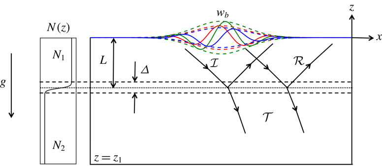
We consider the two-dimensional set-up presented in figure 1. The physical domain extends from
 $-\infty$
to
 $+\infty$
in the
 $x$
direction, localized velocity forcing is applied at
 $z=0$
and internal waves generated by this forcing can propagate downwards freely through
 $z=z_{1}$
. Although the method is applicable to arbitrary stratifications, to begin we consider a buoyancy frequency profile
 $N(z)=\sqrt{(-g/\unicode[STIX]{x1D70C}_{0})\,\text{d}\bar{\unicode[STIX]{x1D70C}}/\text{d}z}$
that changes from a value of
 $N_{1}$
to
 $N_{2}$
through a transition layer of thickness
 $\unicode[STIX]{x1D6E5}$
that lies a distance
 $L$
below
 $z=0$
; here,
 $\unicode[STIX]{x1D70C}_{0}$
is the characteristic density of the fluid,
 $\bar{\unicode[STIX]{x1D70C}}$
is the background density and
 $g$
is the gravitational acceleration. More specifically, the form of the stratification profile that is considered for our case study in § 3 is
 $$\begin{eqnarray}N(z)=\left(\frac{N_{1}+N_{2}}{2}\right)+\left(\frac{N_{1}-N_{2}}{2}\right)\tanh \left(\frac{z+L}{\unicode[STIX]{x1D6E5}/6}\right).\end{eqnarray}$$
The profile given by (2.1) is chosen such that the buoyancy frequency attains the values
 $N_{1}$
and
 $N_{2}$
at
 $z=-L+\unicode[STIX]{x1D6E5}/2$
and
 $z=-L-\unicode[STIX]{x1D6E5}/2$
, respectively, to within 0.1 %.
Sketch of the physical system. The coloured solid lines indicate the vertical velocity forcing function at times
 $t_{-}$
(red),
 $t_{0}$
(green) and
 $t_{+}$
(blue) such that
 $t_{-}<t_{0}<t_{+}$
. The dashed lines indicate the corresponding Gaussian envelopes. Solid lines with arrows define approximate boundaries of the internal wave packets, while the arrows indicate the direction of the group velocity.

To investigate the effects of spatiotemporal localization, we consider a vertical velocity forcing function given by
 $$\begin{eqnarray}w_{b}(x,t)=\text{Re}\left\{A\exp (\text{i}(k_{0}x-\unicode[STIX]{x1D714}_{0}t))\exp \left(\frac{-(x-x_{0})^{2}}{2\unicode[STIX]{x1D70E}_{x}^{2}}\right)\exp \left(\frac{-(t-t_{0})^{2}}{2\unicode[STIX]{x1D70E}_{t}^{2}}\right)\right\},\end{eqnarray}$$
which is applied at
 $z=0$
. The function (2.2) can be viewed as a travelling wave of amplitude
 $A$
modulated by Gaussian envelopes in both space and time that attain their peak values at
 $x=x_{0}$
and
 $t=t_{0}$
, respectively; the modulation broadens the wavenumber and frequency content of the forcing around
 $k_{0}$
and
 $\unicode[STIX]{x1D714}_{0}$
, depending on the magnitude of the widths of the Gaussian functions given by
 $\unicode[STIX]{x1D70E}_{x}$
and
 $\unicode[STIX]{x1D70E}_{t}$
, respectively. The form of the forcing function at times before, at and after the temporal Gaussian peak is illustrated in figure 1. The phase velocity has the magnitude
 $\unicode[STIX]{x1D714}_{0}/k_{0}$
and is directed along the
 $+x$
axis. The forcing will thus induce an incident, rightward-propagating wave packet (
 ${\mathcal{I}}$
) with a downward group velocity. This wave packet then experiences reflection (
 ${\mathcal{R}}$
) and transmission (
 ${\mathcal{T}}$
) as a result of encountering the transition layer as indicated in figure 1.
The dynamics of two-dimensional, linear internal waves propagating in a viscous stratified fluid is governed by Sutherland (Reference Sutherland2010)
 $$\begin{eqnarray}(\unicode[STIX]{x1D6FB}^{2}w)_{tt}+N(z)^{2}w_{xx}=\unicode[STIX]{x1D708}(\unicode[STIX]{x1D6FB}^{4}w)_{t}.\end{eqnarray}$$
Here,
 $w$
is the vertical velocity field and
 $\unicode[STIX]{x1D708}$
is the kinematic viscosity of the fluid. For a given forcing function, we solve (2.3) by performing a Fourier decomposition of the forcing function in
 $x$
and
 $t$
. A general vertical velocity forcing function that is imposed as a boundary condition at
 $z=0$
can be decomposed into its Fourier modes as follows:
 $$\begin{eqnarray}w_{b}(x,t)=\int _{-\infty }^{+\infty }\int _{-\infty }^{+\infty }\widehat{w}_{b}(k,\unicode[STIX]{x1D714})\text{e}^{\text{i}(kx-\unicode[STIX]{x1D714}t)}\,\text{d}k\,\text{d}\unicode[STIX]{x1D714}.\end{eqnarray}$$
For a Fourier mode of the forcing corresponding to the horizontal wavenumber
 $k$
and frequency
 $\unicode[STIX]{x1D714}$
, we substitute an ansatz
 $\widehat{w}(z)\exp (\text{i}(kx-\unicode[STIX]{x1D714}t))$
for
 $w(x,z,t)$
in (2.3) to obtain (Ghaemsaidi et al.
Reference Ghaemsaidi, Dosser, Rainville and Peacock2016a
)
 $$\begin{eqnarray}\widehat{w}_{zzzz}+\left(\frac{\text{i}\unicode[STIX]{x1D714}}{\unicode[STIX]{x1D708}}-2k^{2}\right)\widehat{w}_{zz}+k^{2}\left(k^{2}+\frac{\text{i}\unicode[STIX]{x1D714}}{\unicode[STIX]{x1D708}}\left(\frac{N(z)^{2}}{\unicode[STIX]{x1D714}^{2}}-1\right)\right)\widehat{w}=0,\end{eqnarray}$$
where
 $k$
and
 $\unicode[STIX]{x1D714}$
are known and
 $\widehat{w}$
can in general be complex. This equation gives us the vertical structure of the velocity field for every Fourier mode of the forcing. As noted by Mathur & Peacock (Reference Mathur and Peacock2009), it is not favourable to solve this equation as an initial value problem because it has a pair of rapidly decaying and growing solutions, which can cause numerical instability. It is thus solved as a boundary value problem with two boundary conditions each at
 $z=0$
and
 $z=z_{1}$
. To find the boundary conditions, we seek solutions of the form
 $\exp (mz)$
to satisfy (2.5) in the regions where
 $N(z)$
is constant to obtain a quartic equation for
 $m$
. In the case where a constant stratification is not completely achieved, the application of this method requires the following Wentzel–Kramers–Brillouin condition to be reasonably satisfied at the depth
 $z=z_{1}$
, where the lower boundary conditions will be applied (Ghaemsaidi et al.
Reference Ghaemsaidi, Dosser, Rainville and Peacock2016a
):
 $$\begin{eqnarray}|m|\gg \left(\frac{k^{2}NN^{\prime }}{\unicode[STIX]{x1D714}^{2}}\right)^{1/3}.\end{eqnarray}$$
In general, there can be four complex roots for
 $m$
, the imaginary part of which is the local vertical wavenumber. Only one of these solutions leads to a downward group velocity and viscous decay. We choose this root in each layer and deduce that
 $\widehat{w}(z)$
must have the following functional forms:
 $\widehat{w}=I\exp (m_{1}z)+R\exp (-m_{1}z)$
in the top layer and
 $\widehat{w}=T\exp (m_{2}z)$
in the bottom layer. Here,
 $I$
,
 $R$
and
 $T$
are the amplitudes of the incident, reflected and transmitted waves through the transition layer, respectively, and
 $m_{1}$
and
 $m_{2}$
are the local complex-valued vertical wavenumbers in the
 $N_{1}$
and
 $N_{2}$
layers, respectively. Given these functional forms, we may apply the following boundary conditions:
 $$\begin{eqnarray}\displaystyle & \displaystyle \widehat{w}=\widehat{w}_{b}\quad \text{at}~z=0, & \displaystyle\end{eqnarray}$$
 $$\begin{eqnarray}\displaystyle & \displaystyle \widehat{w}_{zz}=m_{1}^{2}\,\widehat{w}\quad \text{at}~z=0, & \displaystyle\end{eqnarray}$$
 $$\begin{eqnarray}\displaystyle & \displaystyle \widehat{w}_{z}=m_{2}\,\widehat{w}\quad \text{at}~z=z_{1}, & \displaystyle\end{eqnarray}$$
 $$\begin{eqnarray}\displaystyle & \displaystyle \widehat{w}_{zz}=m_{2}^{2}\,\widehat{w}\quad \text{at}~z=z_{1}. & \displaystyle\end{eqnarray}$$
 $z=0$
is specified by the forcing. Equations (2.7b
), (2.7c
) and (2.7d
) ensure the exponential
 $z$
dependence of the excited internal waves with the correct vertical wavenumber. If
 $z_{1}\rightarrow -\infty$
, (2.7d
) is indeed a redundant condition. However, for the problem with a finite bottom, it closes the system numerically.
The decomposition given by (2.4) is performed numerically using the fast Fourier transform algorithm. Thereafter, for the obtained discrete Fourier modes of the forcing, we numerically solve (2.5) with (2.7) using the MATLAB bvp4c solver. After obtaining the vertical structures
 $\widehat{w}(z;\unicode[STIX]{x1D714},k)$
for each Fourier mode, we transform them back to the space–time domain by taking an inverse Fourier transform to obtain the vertical velocity field
 $w(x,z,t)$
. The other field variables such as the stream function
 $\unicode[STIX]{x1D713}$
, horizontal velocity
 $u$
, pressure
 $p$
and density perturbation
 $\unicode[STIX]{x1D70C}$
can be found via the linear modal relations:
 $$\begin{eqnarray}\displaystyle & \displaystyle \widehat{\unicode[STIX]{x1D713}}(z)=\frac{-\text{i}\widehat{w}}{k}, & \displaystyle\end{eqnarray}$$
 $$\begin{eqnarray}\displaystyle & \displaystyle \widehat{u}(z)=-\widehat{\unicode[STIX]{x1D713}}_{z}, & \displaystyle\end{eqnarray}$$
 $$\begin{eqnarray}\displaystyle & \displaystyle \widehat{p}(z)=\frac{\unicode[STIX]{x1D70C}_{0}}{k}(-\unicode[STIX]{x1D714}\widehat{\unicode[STIX]{x1D713}}_{z}-\text{i}\unicode[STIX]{x1D708}(\widehat{\unicode[STIX]{x1D713}}_{zz}-k^{2}\widehat{\unicode[STIX]{x1D713}})), & \displaystyle\end{eqnarray}$$
 $$\begin{eqnarray}\displaystyle & \displaystyle \widehat{\unicode[STIX]{x1D70C}}(z)=\frac{\text{i}\unicode[STIX]{x1D70C}_{0}kN^{2}}{g}\widehat{\unicode[STIX]{x1D713}}. & \displaystyle\end{eqnarray}$$
This method of Fourier decomposition works if the excited velocity field is also localized. That is, its magnitude goes to zero at the end time in the entire domain which is possible due to the bottom boundary condition as we allow for the waves to escape. When the waves are propagating (
 $\unicode[STIX]{x1D714}<N_{1},N_{2}$
), the end time and the domain size in
 $x$
need to be chosen such that all of the wave energy escapes through the bottom without reaching the side-ends of the domain. If this is not the case, due to the intrinsic periodic nature of using Fourier modes, there can be spurious waves appearing at
 $t=0$
. An issue arises when
 $N_{2}<\unicode[STIX]{x1D714}<N_{1}$
, which implies that the waves are propagating in the upper layer but evanescent in the lower layer. We discuss this specific scenario as it is encountered in the laboratory experiments that are discussed in § 4. Because the internal waves cannot propagate through the lower layer, they undergo multiple reflections off the transition layer and the upper boundary. All of the forced input energy then gets focused in the upper layer. The only way by which the wave energy can progressively decrease is through viscous dissipation. Solutions to (2.5) ensure that there is viscous decay along the direction of propagation of the internal waves. Therefore, the domain size in
 $x$
and the chosen time window have to be large enough so that the waves are dissipated entirely within the domain. Subsequently, we also conclude that for this particular scenario
 $(N_{2}<\unicode[STIX]{x1D714}<N_{1})$
, the method of Fourier decomposition cannot provide us with an inviscid solution.
3 Model results
3.1 Case study
We begin by considering an inviscid system with the stratification parameters
 $\unicode[STIX]{x1D6E5}/L=0.5$
and
 $N_{2}/N_{1}=0.6$
, wave field parameters
 $\unicode[STIX]{x1D714}_{0}/N_{1}=0.52$
and
 $k_{0}L=4.8$
and localization parameters
 $\unicode[STIX]{x1D70E}_{t}N_{1}=22.5$
and
 $\unicode[STIX]{x1D70E}_{x}/L=2$
(here, we use the time scale
 $1/N_{1}$
and length scale
 $L$
to non-dimensionalize the localization parameters for convenience only; the correct non-dimensionalization of
 $\unicode[STIX]{x1D70E}_{x}$
and
 $\unicode[STIX]{x1D70E}_{t}$
is discussed in § 3.2). For these parameters, the spatiotemporal nature of the forcing and the vertical velocity field are presented in figure 2. At the time instant shown, the forcing time window has passed and has excited a wave packet
 ${\mathcal{I}}_{1}$
that has interacted with the transition layer to result in the reflected wave packet
 ${\mathcal{R}}_{1}$
and transmitted wave packet
 ${\mathcal{T}}_{1}$
. The wave packet
 ${\mathcal{R}}_{1}$
interferes with the forcing at
 $z=0$
and gets reflected back towards the transition layer as the wave packet
 ${\mathcal{I}}_{2}$
. This wave packet gets transmitted through the transition layer as
 ${\mathcal{T}}_{2}$
and reflected as
 ${\mathcal{R}}_{2}$
. If the forcing is harmonic in time and space and the parameters permit constructive interference (as they do in this case), the amplitude would be non-negligible for an infinite number of such reflections. However, due to the spatiotemporal localization, we observe that the amplitude has greatly decreased even for the second reflected wave packet
 ${\mathcal{R}}_{2}$
.
Forcing and the excited vertical velocity field for validation case study at
 $tN_{1}=135$
. (a) Spatiotemporal nature of the velocity forcing at
 $z=0$
, wherein the horizontal line indicates
 $tN_{1}=135$
, the time for which panel (b) is plotted. (b) Vertical velocity field in the domain at
 $tN_{1}=135$
. The arrows indicate the group velocities of the respective wave packets and the corresponding labels are to their left. (c) Stratification profile. Dotted lines in panel (b) indicate the transition region.

We now define the parameter
 $\unicode[STIX]{x1D6E4}$
to be
 $$\begin{eqnarray}\unicode[STIX]{x1D6E4}=\max |w|/A\quad \text{at}~z/L=-1-0.5\unicode[STIX]{x1D6E5}/L,\end{eqnarray}$$
which is the maximum vertical velocity amplitude immediately below the transition layer as compared to the forcing amplitude. If
 $\unicode[STIX]{x1D714}_{0}<N_{2}$
, we have freely propagating waves in the bottom layer, in which case
 $\unicode[STIX]{x1D6E4}$
represents true transmission. Otherwise, if the waves are evanescent in the bottom layer,
 $\unicode[STIX]{x1D6E4}$
is a proxy for measuring the amount of interference in the upper layer. For this case study,
 $\unicode[STIX]{x1D714}_{0}<N_{2}$
and
 $\unicode[STIX]{x1D6E4}$
is determined to be 1.56; for comparison, for harmonic forcing (that is,
 $\unicode[STIX]{x1D70E}_{t},\unicode[STIX]{x1D70E}_{x}\rightarrow \infty$
) with the same forcing parameters, the parameter
 $\unicode[STIX]{x1D6E4}=2.53$
(
 $\simeq 62\,\%$
larger), indicating a greater degree of constructive interference. This can be corroborated by identifying that at the time the bulk of the reflected wave packet
 ${\mathcal{R}}_{1}$
reaches
 $z=0$
, the forcing has a diminished amplitude due to temporal localization. Additionally, the reflected wave packet arrives at the
 $z=0$
level to the right of the forcing where the amplitude is diminished due to spatial localization. Thus, the spatiotemporal localization reduces the amount of interference that can happen between the reflected wave packet and the forcing itself in the
 $N_{1}$
layer. There is a further reduction in the forcing amplitude by the time the wave packet
 ${\mathcal{R}}_{2}$
reaches
 $z=0$
. One can also think of it from the frequency and wavenumber domain. Due to the localization, we introduce a band of wavenumbers and frequencies that have their own coefficients of transmission for this system. The total coefficient of transmission is thus a combination of these individual coefficients and the Fourier amplitudes of the forcing. If the dominant wavenumber and frequency lie on a harmonic transmission peak, the transmission for a localized forcing is expected to be lower due to the contribution of wavenumbers and frequencies around that do not lie on the harmonic transmission peak.
We now proceed to use the theoretical model to perform parametric studies to investigate how the forcing parameters affect the transmission of the system. Intuitively, we expect that as the size of the forcing gets larger both spatially and temporally, effects of interference will be enhanced as a greater number of reflections can now interfere with the forcing. This would also depend on the dominant frequency and wavenumber, however, as the propagation angle and the group velocity of the waves depend on these factors.
3.2 Effects of localization
Using a ray approach for a discontinuous stratification profile, it has been shown that as the number of reflections increases, the effect of either constructive or destructive interference becomes more and more pronounced (Ghaemsaidi Reference Ghaemsaidi2015). In the case of a spatially localized forcing, only a finite number of reflections actually interact with the forcing and, similarly, if the forcing is temporally localized the time for which the forcing exists only permits a limited number of reflections to interfere. Adopting this perspective, we will define a new characteristic length scale
 $L^{\ast }$
and a time scale
 $t^{\ast }$
, with a view to developing practical criteria for when interference effects will be evident. Supekar (Reference Supekar2017) found these scales to be
 $$\begin{eqnarray}\displaystyle & L^{\ast }=2L\cot \unicode[STIX]{x1D703}_{0}, & \displaystyle\end{eqnarray}$$
 $$\begin{eqnarray}\displaystyle & t^{\ast }=(2L/\text{sin}\,\unicode[STIX]{x1D703}_{0})/c_{g}. & \displaystyle\end{eqnarray}$$
 $L^{\ast }$
is the horizontal distance between the point at which a wave packet leaves the
 $z=0$
level and the point at which it finds itself upon returning after getting reflected off the transition region,
 $t^{\ast }$
is the corresponding travel time that the wave packet takes,
 $\unicode[STIX]{x1D703}_{0}=\sin ^{-1}(\unicode[STIX]{x1D714}_{0}/N_{1})$
is the angle of wave packet propagation with respect to the horizontal in the upper layer and
 $c_{g}=N_{1}\sin \unicode[STIX]{x1D703}_{0}\cos \unicode[STIX]{x1D703}_{0}/k_{0}$
is the group velocity. All these quantities are defined for the dominant frequency and wavenumber. We then define the following dimensionless parameters:
 $$\begin{eqnarray}\displaystyle & n_{x}=4\unicode[STIX]{x1D70E}_{x}/L^{\ast }, & \displaystyle\end{eqnarray}$$
 $$\begin{eqnarray}\displaystyle & n_{t}=4\unicode[STIX]{x1D70E}_{t}/t^{\ast }, & \displaystyle\end{eqnarray}$$
 $n_{x}$
and
 $n_{t}$
reasonably quantify the number of reflections that the spatiotemporal extent of the forcing supports for interference; the factor of 4 ensures that 95 % of the spatiotemporal extent of the forcing is considered. It is to be expected that interference effects present in the case of harmonic forcing will be evident only when both
 $n_{x}$
and
 $n_{t}$
are above a certain threshold.
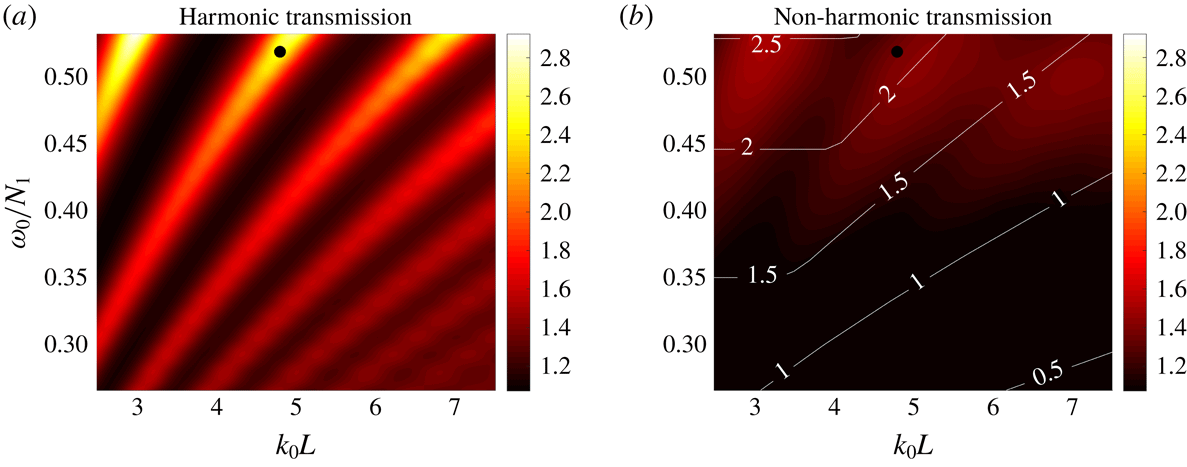
To explore these ideas, we consider the results for the parameter
 $\unicode[STIX]{x1D6E4}$
for the harmonic and non-harmonic forcing, presented in figure 3. For a harmonic forcing, the transmission peaks and troughs can be clearly seen, achieving maximum values of
 $\unicode[STIX]{x1D6E4}\simeq 3$
. A similar transmission spectrum was obtained by Gregory & Sutherland (Reference Gregory and Sutherland2010) in a slightly different system for internal wave beams and Mathur & Peacock (Reference Mathur and Peacock2009) have studied the influence of the transition layer width
 $\unicode[STIX]{x1D6E5}$
on the transmission. In contrast, the transmission plot for localized forcing, which is overlaid by contours of the function
 $\min \{n_{x},n_{t}\}$
, displays identifiable peaks only when
 $n_{x},n_{t}>1.5$
(approximately); below this threshold, the transmission peaks disappear. That is, there needs to be enough spatiotemporal extent for at least one reflected wave packet to interfere with the forcing. Furthermore, the maximum value of the parameter
 $\unicode[STIX]{x1D6E4}$
is notably reduced to
 $\unicode[STIX]{x1D6E4}\simeq 1.5$
. Parameters for the motivating example are indicated by black circles in figure 3. It is clear that if the forcing were harmonic, the frequency and wavenumber pair lies on a transmission peak. In the case of a non-harmonic forcing, the parameter
 $\unicode[STIX]{x1D6E4}$
gets smaller in the interference peaks and larger in the troughs as compared to the respective harmonic cases. Hence, for the example under consideration, the transmission parameter decreases.
Comparison of the transmission
 $\unicode[STIX]{x1D6E4}$
(for
 $\unicode[STIX]{x1D6E5}/L=0.5$
,
 $N_{2}/N_{1}=0.6$
). (a) The transmission spectra for harmonic forcing. (b) The transmission spectra for a localized forcing with
 $\unicode[STIX]{x1D70E}_{t}N_{1}=22.5$
and
 $\unicode[STIX]{x1D70E}_{x}/L=2$
; the contours indicate the function
 $\min \{n_{x},n_{t}\}$
. The black circles in (a) and (b) indicate the forcing parameters considered for the motivating example.

Effect of temporal delocalization on (a) the transmission
 $\unicode[STIX]{x1D6E4}$
and (b) the total energy transferred (for
 $\unicode[STIX]{x1D6E5}/L=0.5$
,
 $N_{2}/N_{1}=0.6$
,
 $\unicode[STIX]{x1D70E}_{x}/L=2$
,
 $k_{0}L=4$
). The colour bar in (a) is set to the be the same as in figure 3. The contours in (a) and (b) correspond to the function
 $\min \{n_{x},n_{t}\}$
.

Figure 4 presents results for the transmission parameter,
 $\unicode[STIX]{x1D6E4}$
, and the energy input to the system,
 ${\mathcal{E}}$
, for a disturbance of fixed spatial nature (
 $k_{0}L=4,\unicode[STIX]{x1D70E}_{x}/L=2$
) and varying temporal extent (
 $15<\unicode[STIX]{x1D70E}_{t}N_{1}<45$
); the total energy transmitted per unit depth (
 ${\mathcal{E}}=\iint (pw)\,\text{d}x\,\text{d}t$
) has been non-dimensionalized by the characteristic scale
 $\unicode[STIX]{x1D70C}_{0}A^{2}L^{2}$
. For
 $\unicode[STIX]{x1D70E}_{t}N_{1}\simeq 15$
, the transmission parameter and the energy input do not vary much as a function of
 $\unicode[STIX]{x1D714}_{0}/N_{1}$
, but as
 $\unicode[STIX]{x1D70E}_{t}N_{1}$
exceeds 25, constructive and destructive interference peaks emerge. Contours of the function
 $\min \{n_{x},n_{t}\}$
are overlaid on both plots and again it is evident that peaks and troughs in both the transmission parameter and the energy input appear only above
 $n_{x},n_{t}>1.5$
.
4 Experiments
4.1 Apparatus
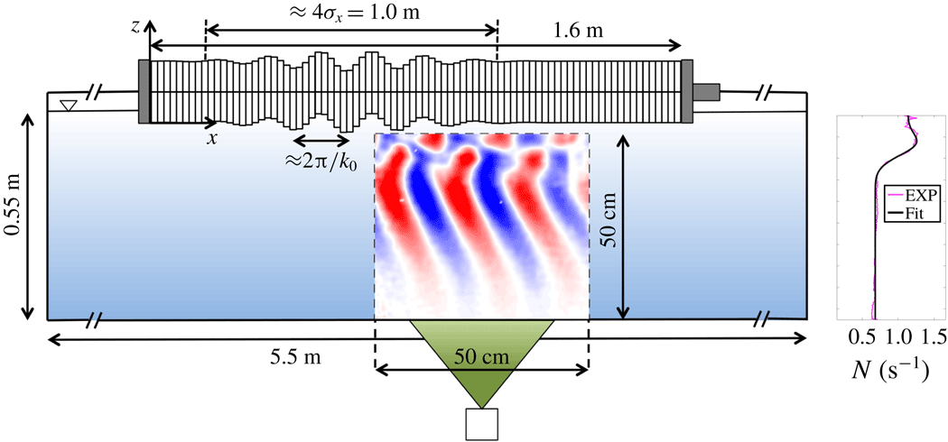
For the experimental studies, we used a glass wave tank that was 5.5 m long, 0.55 m wide and 0.55 m high. A schematic of the front view of the set-up is shown in figure 5. The tank was separated by a partition that ran along its length creating a working section which was 0.2 m wide. There were parabolic reflectors at the ends of the tank that reflected any waves that were generated in the working section of the tank so that they were dissipated behind the partition (Echeverri Reference Echeverri2009).
Schematic of the front view of the experimental set-up. The observation region is indicated by dotted lines and it is illuminated from underneath the tank by the laser sheet that is depicted in green. An example vertical velocity field that is obtained from PIV is indicated within the dotted lines.

Salt-stratified water was used to set up the density stratification using the double-bucket method (Oster Reference Oster1965), for which the flow rates out of the two buckets were controlled using two peristaltic pumps. The flow rate from the dense water bucket to the freshwater bucket and that from the freshwater bucket to the experimental tank were maintained at 3 and 6
 $\text{l}~\text{min}^{-1}$
. As a result of the stratification, density in the tank varied between roughly
 $1000$
and
 $1040~\text{kg}~\text{m}^{-3}$
. A Precision Measurements Engineering conductivity probe was calibrated and used to measure the density profile. The calculated buoyancy frequency from the raw density profile is plotted in figure 5. This profile differs a little from the profile given by (2.1). The small bump in the buoyancy frequency just above the transition region occurred due to experimental limitations of changing the volumes of water in the buckets in the double-bucket method. Nevertheless, we account for this difference by fitting a function of the following form:
 $$\begin{eqnarray}N(z)=\left(\frac{N_{1}+N_{2}}{2}\right)+\left(\frac{N_{1}-N_{2}}{2}\right)\tanh \left(\frac{z+L}{\unicode[STIX]{x1D6E5}/6}\right)+(N_{3}-N_{1})\exp \left(-\frac{1}{2}\left[\frac{z+L}{\unicode[STIX]{x1D6E5}/6}\right]^{2}\right).\end{eqnarray}$$
This function is essentially the one defined by (2.1) superimposed with a Gaussian function in the transition region. By performing a least-squares fit to the experimental data, the parameters were found to be
 $N_{1}=1.14~\text{s}^{-1}$
,
 $N_{2}=0.685~\text{s}^{-1}$
,
 $N_{3}=1.41~\text{s}^{-1}$
,
 $\unicode[STIX]{x1D6E5}=16.0~\text{cm}$
and
 $L=7.8~\text{cm}$
. As shown in figure 5, this function approximates the experimental buoyancy frequency profile very well and is thus used for predictions from the theoretical model. Due to the existence of the bump, there could be modes that are trapped and horizontally propagating, which are taken into account as the modal equation (2.5) is solved numerically.
The velocity field of the generated internal waves was measured using particle image velocimetry (PIV) in a
 $50~\text{cm}\times 50~\text{cm}$
observation region as indicated in figure 5. Hollow glass spheres with a diameter of
 $8{-}10~\unicode[STIX]{x03BC}\text{m}$
were used to seed the flow. A light sheet was created from underneath the tank using a pulsed Nd : YAG laser. Images of the seeding particles were recorded using an Imager Pro X 4M LaVision CCD camera at a resolution of
 $2042\times 2042$
and at a rate of 32 images per forcing period. Since the flow velocities are of the order of a few millimetres per second, a single laser head was pulsed and cross-correlation was performed between consecutive particle images. The post-processing and calibration of the cameras were done using the DaVis PIV software developed by LaVision. An example experimental vertical velocity field overlaid on the experimental schematic is shown in figure 5.
4.2 Wave generator configuration
In order to force the internal waves, we used a wave generator that was built based on the design by Gostiaux et al. (Reference Gostiaux, Didelle, Mercier and Dauxois2007) which was also analysed by Mercier et al. (Reference Mercier, Martinand, Mathur, Gostiaux, Peacock and Dauxois2010). The wave generator was set up on top of the tank as shown in figure 5. It consisted of 84 individual plates whose vertical position is controlled by individual circular cams whose centres can be offset from the spindle centre. The eccentricity (
 $e_{j}$
) and phase (
 $\unicode[STIX]{x1D719}_{j}$
) of the cams were adjusted individually, where
 $j$
indicates the serial number of the plates. The eccentricities
 $e_{j}$
were set to a maximum value of
 $e=5~\text{mm}$
. The cams were attached to a spindle that was rotated by a motor at variable speed (angular position of the spindle is given by
 $\unicode[STIX]{x1D6FE}(t)$
). The time-dependent vertical velocity of each plate can be expressed as
 $$\begin{eqnarray}w_{j}(t)=e_{j}\cos (\unicode[STIX]{x1D719}_{j}+\unicode[STIX]{x1D6FE}(t))\,\text{d}\unicode[STIX]{x1D6FE}/\text{d}t.\end{eqnarray}$$
The wave generator provided two degrees of freedom in the horizontal spatial direction (eccentricity and phase) but only one in time (
 $\unicode[STIX]{x1D6FE}(t)$
). Hence, getting a temporally localized velocity profile that is smooth was non-trivial. Also, to set the wave generator to realize a specific spatial profile, all of the plates and cams need to be removed and configured individually. This limited our ability to vary the spatial parameters of the forcing through an experiment. Therefore, we chose to fix the spatial profile and vary the temporal parameters alone with frequency and time window of the forcing. The spatial Gaussian envelope of the idealized forcing function given by (2.2) was physically realized by setting
 $e_{j}=e\exp (-(x_{j}-x_{0})^{2}/2\unicode[STIX]{x1D70E}_{x}^{2})$
and
 $\unicode[STIX]{x1D719}_{j}=k_{0}x_{j}$
. Since the rotation of all the cams is given by a single function
 $\unicode[STIX]{x1D6FE}(t)$
, however, it was not possible to exactly reproduce the temporal part of the function in (2.2). We thus utilized the following function for
 $\unicode[STIX]{x1D6FE}(t)$
, such that
 $\text{d}\unicode[STIX]{x1D6FE}/\text{d}t$
forms a localized temporal envelope:
 $$\begin{eqnarray}\unicode[STIX]{x1D6FE}(t)=\frac{\unicode[STIX]{x1D714}_{0}}{2}\int _{0}^{t}\left[\tanh \left(\frac{\bar{t}-(t_{0}-\unicode[STIX]{x1D70E}_{t}/2)}{\unicode[STIX]{x1D6FF}/6}\right)-\tanh \left(\frac{\bar{t}-(t_{0}+\unicode[STIX]{x1D70E}_{t}/2)}{\unicode[STIX]{x1D6FF}/6}\right)\right]\text{d}\bar{t}.\end{eqnarray}$$
Such a definition ensured that
 $\unicode[STIX]{x1D6FE}(t)$
changes monotonically, and hence the phase speed was always directed in the same direction. The phase speed of the forcing increases from zero to a maximum value of
 $(\unicode[STIX]{x1D714}_{0}/k_{0})$
over a time given by
 $\unicode[STIX]{x1D6FF}$
. It stayed at the maximum value for a time of about
 $\unicode[STIX]{x1D70E}_{t}$
and reduced back to zero in
 $\unicode[STIX]{x1D6FF}$
. Nevertheless, such a
 $\unicode[STIX]{x1D6FE}(t)$
profile gave us a temporally localized forcing with a broad frequency spectrum close to but not exactly
 $\unicode[STIX]{x1D714}_{0}$
. The forcing is also symmetric about the time
 $t_{0}$
which we will refer to as the mean time of the forcing. An example angular velocity (
 $\text{d}\unicode[STIX]{x1D6FE}/\text{d}t$
) profile is shown in figure 6. The Fourier transform of the plate velocity indicates that it has a peak at
 $\pm \unicode[STIX]{x1D714}_{0}$
and is fairly symmetric about the peak. The function given by (4.3) thus served adequate for verifying our theoretical predictions.
An example of the temporal part of the wave generator forcing given by (4.3). (a) The angular velocity (
 $\text{d}\unicode[STIX]{x1D6FE}/\text{d}t$
) of the motor for the following set of experimental parameters:
 $\unicode[STIX]{x1D714}_{0}=0.68~\text{s}^{-1}$
,
 $\unicode[STIX]{x1D70E}_{t}=50~\text{s}$
,
 $t_{0}=40~\text{s}$
,
 $\unicode[STIX]{x1D6FF}=20~\text{s}$
,
 $e=5~\text{mm}$
. (b) The vertical position and velocity of a single generator plate. (c) The amplitude of the Fourier transform of the plate vertical velocity
 $w_{j}$
, wherein the dotted red lines indicate
 $\pm \unicode[STIX]{x1D714}_{0}$
.

The stepper motor on the wave generator was controlled using a LabView program and an NI (National Instruments) motion controller to attain the intricate
 $\unicode[STIX]{x1D6FE}(t)$
profile. For the experimental runs, the wave generator was configured such that
 $k_{0}=40.69~\text{m}^{-1}$
and
 $\unicode[STIX]{x1D70E}_{x}=0.25~\text{m}$
and
 $\unicode[STIX]{x1D714}_{0}$
and
 $\unicode[STIX]{x1D70E}_{t}$
were varied. The choice of
 $k_{0}$
was made so as to ensure that the Reynolds number associated with the excited waves is not too small that viscous effects are highly dominant. A large value of
 $k_{0}$
would result in a larger viscous dissipation as the viscous decay rate is proportional to
 $k_{0}^{3}$
. For the chosen value of the wavenumber, the Reynolds number,
 $Re=A\unicode[STIX]{x1D714}_{0}/\unicode[STIX]{x1D708}k_{0}$
, was of the order of (10–100).
4.3 Results
For the stratification that was set up, we performed a total of 43 experimental runs where only the temporal part of the forcing that is given by
 $\unicode[STIX]{x1D6FE}(t)$
in (4.3) was varied. The value of
 $\unicode[STIX]{x1D6FF}$
was set to 20 s. The dominant frequency
 $\unicode[STIX]{x1D714}_{0}$
was varied from
 $0.68$
to
 $1.28~\text{s}^{-1}$
for three different values of
 $\unicode[STIX]{x1D70E}_{t}$
, i.e. 20, 50 and 200 s. This range of frequencies was especially chosen so that the internal waves in the bottom layer are evanescent. Such a scenario ensures that all of the forced energy is concentrated in the upper layer, thus leading to resonant peaks in the
 $\unicode[STIX]{x1D6E4}$
versus
 $\unicode[STIX]{x1D714}_{0}$
curve for a harmonic forcing (Ghaemsaidi Reference Ghaemsaidi2015). Thus, it allows us to experimentally verify the peaks in the spectrum of the parameter
 $\unicode[STIX]{x1D6E4}$
, which is otherwise challenging when the waves are freely propagating in the bottom layer as the peaks are not strong enough for a non-harmonic forcing (see figure 3). The value of the mean time
 $t_{0}$
was chosen on the basis of
 $\unicode[STIX]{x1D70E}_{t}$
(
 $t_{0}=25$
, 40 and 115 s for
 $\unicode[STIX]{x1D70E}_{t}=20$
, 50 and 200 s, respectively). To better resolve the expected peaks when
 $\unicode[STIX]{x1D70E}_{t}=200~\text{s}$
, we performed experiments for 21 different values of
 $\unicode[STIX]{x1D714}_{0}$
that were equally spaced in the specified range. For
 $\unicode[STIX]{x1D70E}_{t}=20$
and 50 s, 11 values of
 $\unicode[STIX]{x1D714}_{0}$
were used each.
4.3.1 Experimental studies for
 $\unicode[STIX]{x1D6E4}$

In order to calculate the parameter
 $\unicode[STIX]{x1D6E4}$
from the experimental data, the vertical velocity field at a depth just below the transition region (specifically, at
 $z=-17~\text{cm}$
) was analysed. This depth was chosen as it lay sufficiently below the transition region so that the results were not affected by the reflection patterns within this region. The top 0.01 % data values over all times and horizontal distances at this depth were found and divided by the forcing amplitude
 $A\unicode[STIX]{x1D714}_{0}$
. The parameter
 $\unicode[STIX]{x1D6E4}$
was defined as the mean of these values and the standard deviation provided a rough error estimate. This method ensured that the measured value was not based on a single data point. The choice of using the top 0.01 % was made so as to ensure that sufficient number of data values were actually considered for this calculation without substantially lowering the calculated value of
 $\unicode[STIX]{x1D6E4}$
due to averaging.
4.3.2 Discussion
We will start by focusing on two different cases with forcing frequencies
 $\unicode[STIX]{x1D714}_{0}=0.68~\text{s}^{-1}$
and
 $\unicode[STIX]{x1D714}_{0}=0.86~\text{s}^{-1}$
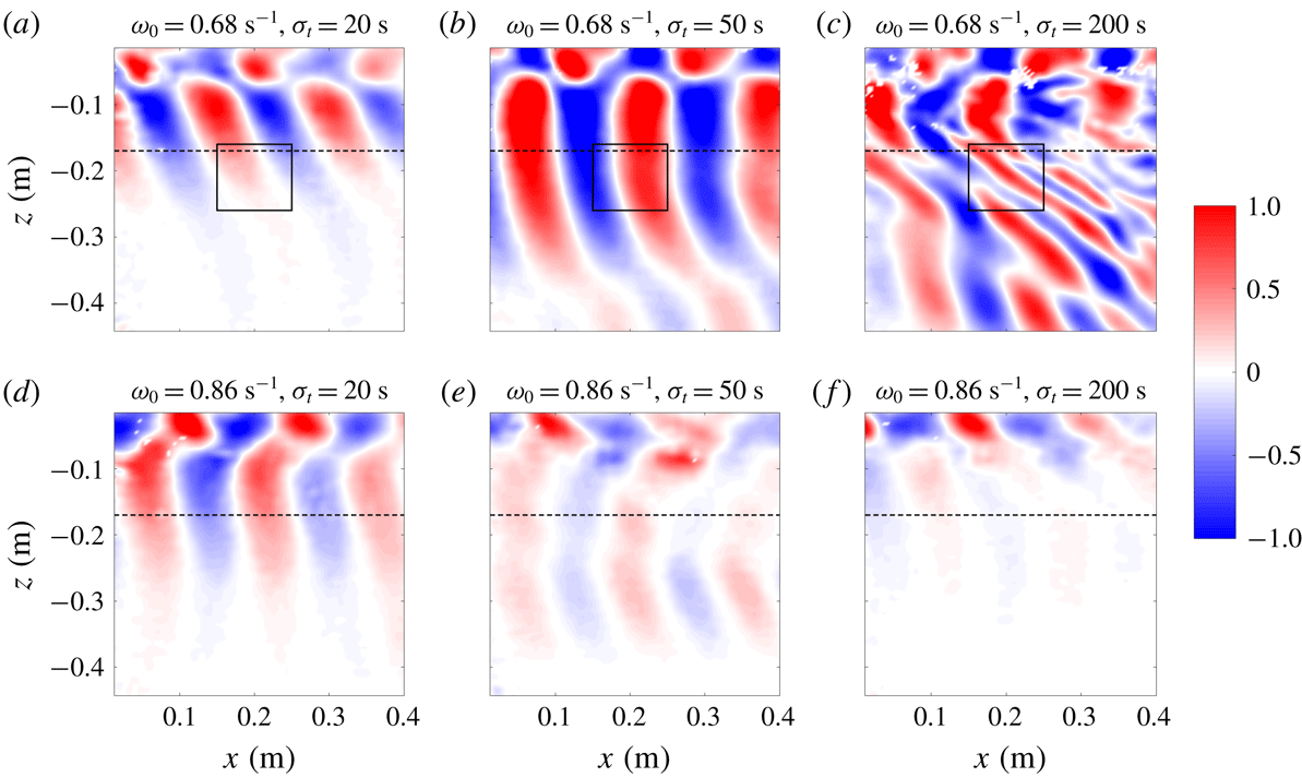
as these two cases resulted in velocity fields that are qualitatively very different. Figure 7 presents the vertical velocity fields at time
 $t=t_{0}+(\unicode[STIX]{x1D70E}_{t}+\unicode[STIX]{x1D6FF})/2$
, which corresponds to the time when the forcing from the wave generator is stopped. The time for which the forcing is active before it is stopped is roughly
 $\unicode[STIX]{x1D70E}_{t}$
, which took the values 20, 50 and 200 s in our experiments. First and foremost, when
 $\unicode[STIX]{x1D714}_{0}=0.68~\text{s}^{-1}$
, it can be seen that as the forcing time window
 $\unicode[STIX]{x1D70E}_{t}$
becomes larger, the velocity field becomes stronger as can be seen in figure 7(a–c). At this frequency, the internal waves that get reflected from the transition region constructively interfere with the forcing which leads to amplification of the wave field over the time for which the forcing is active. To demonstrate this, we plot the parameter
 $\unicode[STIX]{x1D6E4}$
at
 $z=-17~\text{cm}$
(over all
 $x$
) as a function of time in figure 8. The predictions of the theoretical model are also plotted for comparison. As can be seen in figure 8(a–c),
 $\unicode[STIX]{x1D6E4}$
initially increases monotonically with time which can be attributed to constructive interference. For larger values of
 $\unicode[STIX]{x1D70E}_{t}$
, the forcing is active for a longer time and thus the maximum value that
 $\unicode[STIX]{x1D6E4}$
reaches is higher. We remark that even though
 $\unicode[STIX]{x1D714}_{0}>N_{2}$
, due to the temporal localization, a finite bandwidth of frequencies exists around the dominant frequency
 $\unicode[STIX]{x1D714}_{0}$
. Thus, a signature of freely propagating waves can be seen in figure 7 below the transition layer.
Plots of the experimental vertical velocity field normalized by the forcing amplitude (
 $w/(A\unicode[STIX]{x1D714}_{0})$
) for
 $\unicode[STIX]{x1D714}_{0}=0.68~\text{s}^{-1}$
, a frequency at which constructive interference occurs (a–c) and
 $\unicode[STIX]{x1D714}_{0}=0.86~\text{s}^{-1}$
, a frequency at which destructive interference occurs (d–f). The buoyancy frequencies in the top and bottom layers are
 $N_{1}=1.14~\text{s}^{-1}$
and
 $N_{2}=0.685~\text{s}^{-1}$
, respectively. The velocity fields are at
 $t=t_{0}+(\unicode[STIX]{x1D70E}_{t}+\unicode[STIX]{x1D6FF})/2$
which is the time at which the forcing stops. The columns from left to right indicate the velocity fields for
 $\unicode[STIX]{x1D70E}_{t}=20$
, 50 and 200 s, respectively. The horizontal dashed lines indicate the depth at which the parameter
 $\unicode[STIX]{x1D6E4}$
is calculated. The rectangles marked by solid lines in (a–c) enclose the regions used to compute the spatial average for spectrograms presented in figure 9. Note that the colour map is saturated.

Comparison of time series of
 $\unicode[STIX]{x1D6E4}$
at a depth
 $z=-17~\text{cm}$
. (a–c) The constructive (
 $\unicode[STIX]{x1D714}_{0}=0.68~\text{s}^{-1}$
) and (d–f) the destructive (
 $\unicode[STIX]{x1D714}_{0}=0.86~\text{s}^{-1}$
) interference scenarios. From left to right, the columns correspond to
 $\unicode[STIX]{x1D70E}_{t}=20$
, 50 and 200 s, respectively.

Comparison of the spatially averaged spectrograms of the vertical velocity normalized by its maximum value (
 $\log _{10}(S(\unicode[STIX]{x1D714},t)/S_{0})$
). Here
 $\unicode[STIX]{x1D70E}_{t}$
takes the values (a) 20 s, (b) 50 s and (c) 200 s for the constructive interference case of
 $\unicode[STIX]{x1D714}_{0}=0.68~\text{s}^{-1}$
. The spectrograms do not start at
 $t=0~\text{s}$
because of the Hamming window size used in evaluating (4.4).

The agreement between the theoretical and experimental
 $\unicode[STIX]{x1D6E4}$
is very good except for the case of the largest time window (
 $\unicode[STIX]{x1D70E}_{t}=200~\text{s}$
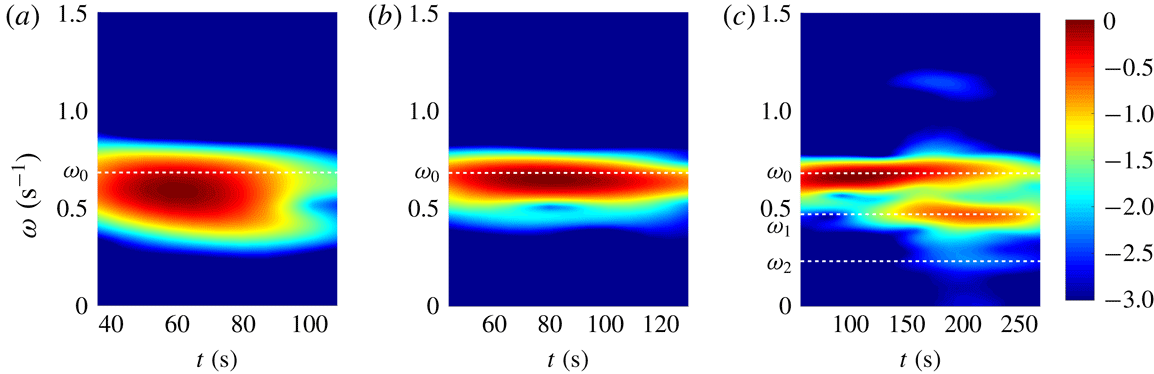
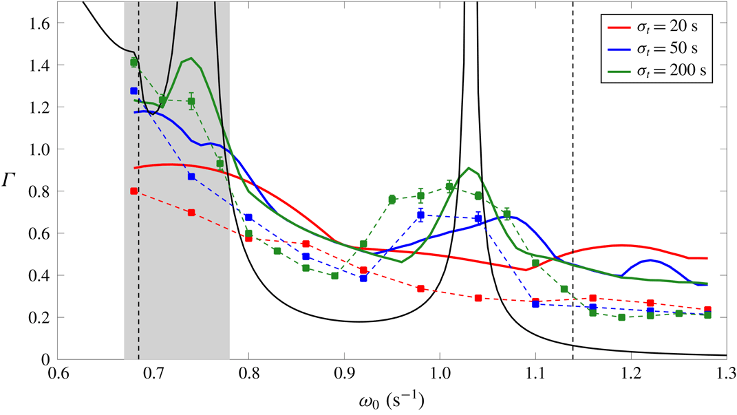
), the mismatch being the largest in the shaded grey region shown in figure 8(c). We argue that this deviation is due to nonlinear effects that our theoretical model does not capture. To demonstrate this, we calculate a spatially averaged spectrogram based on the vertical velocity given by
 $$\begin{eqnarray}S(\unicode[STIX]{x1D714},t)=\left\langle \left|\int _{-\infty }^{\infty }w(\unicode[STIX]{x1D70F})h(t-\unicode[STIX]{x1D70F})\exp (-\text{i}\unicode[STIX]{x1D714}\unicode[STIX]{x1D70F})\,\text{d}\unicode[STIX]{x1D70F}\right|^{2}\right\rangle _{xz},\end{eqnarray}$$
where
 $h$
represents a Hamming window. Spectrograms for the case of
 $\unicode[STIX]{x1D714}_{0}=0.68~\text{s}^{-1}$
and different values of
 $\unicode[STIX]{x1D70E}_{t}$
are shown in figure 9. As the time window
 $\unicode[STIX]{x1D70E}_{t}$
gets larger, the band of frequencies around the dominant frequency
 $\unicode[STIX]{x1D714}_{0}$
gets smaller as expected. In the case of
 $\unicode[STIX]{x1D70E}_{t}=200~\text{s}$
in figure 9(c), at times larger than
 $t\simeq 100~\text{s}$
when the experimental
 $\unicode[STIX]{x1D6E4}$
deviates from the theoretical prediction, in addition to the dominant frequency
 $\unicode[STIX]{x1D714}_{0}$
, the spectrogram has two peaks at the subharmonic frequencies of
 $\unicode[STIX]{x1D714}_{1}\simeq 0.47~\text{s}^{-1}$
and
 $\unicode[STIX]{x1D714}_{2}\simeq 0.23~\text{s}^{-1}$
. We attribute this to the development of parametric subharmonic instability (PSI) due to wave–wave interactions which has been earlier reported in similar physical systems by Ghaemsaidi et al. (Reference Ghaemsaidi, Joubaud, Dauxois, Odier and Peacock2016b
). As is the case with PSI, the parent frequency and the subharmonic frequencies form a resonant triad, that is,
 $\unicode[STIX]{x1D714}_{1}+\unicode[STIX]{x1D714}_{2}\simeq \unicode[STIX]{x1D714}_{0}$
. Parametric subharmonic instability effectively transfers energy from longer to shorter length scales. A reduction in the vertical length scale can be seen in the vertical velocity field shown in figure 7(c). Occurrence of PSI allows for the leakage of energy to the bottom layer as the daughter waves have a frequency lower than the parent frequency. We also note that since we are considering temporally localized forcings, the internal wave field contains a band of frequencies that can potentially lead to wave–wave interactions. When the forcing is highly localized, however, despite the frequency band being large, there is not enough time for the instabilities to grow. This could be the reason why we did not observe any instabilities in the experiments corresponding to
 $\unicode[STIX]{x1D70E}_{t}=20~\text{s}$
or
 $\unicode[STIX]{x1D70E}_{t}=50~\text{s}$
.
We now turn our attention to the frequency
 $\unicode[STIX]{x1D714}_{0}=0.86~\text{s}^{-1}$
, the velocity fields corresponding to which are shown in figure 7(d–f). These velocity fields qualitatively differ from the ones at
 $\unicode[STIX]{x1D714}_{0}=0.68~\text{s}^{-1}$
in that the maximum vertical velocity amplitude indicated by
 $\unicode[STIX]{x1D6E4}$
decreases as the time window
 $\unicode[STIX]{x1D70E}_{t}$
becomes larger. At this frequency, the reflected internal waves destructively interfere with the forcing. Thus, for a larger forcing time window, a larger diminution of the velocity field occurs. We also do not observe any instabilities arising in this case, even for the largest time window. The experimental
 $\unicode[STIX]{x1D6E4}$
is compared with the theoretical predictions in figure 8(d–f), and we find a very good agreement for all the time windows. The diminution of the wave field due to destructive interference prevents the growth of instabilities as the wave field is not strong enough for any nonlinear effects to proliferate.
Theoretical and experimental
 $\unicode[STIX]{x1D6E4}$
for different values of the temporal parameters
 $\unicode[STIX]{x1D70E}_{t}$
and
 $\unicode[STIX]{x1D714}_{0}$
. The red, blue and green solid lines are the theoretical curves for a localized forcing while the solid black line corresponds to a harmonic forcing (
 $\unicode[STIX]{x1D70E}_{x},\unicode[STIX]{x1D70E}_{t}\rightarrow \infty$
). The square markers indicate the experimental
 $\unicode[STIX]{x1D6E4}$
values with the colours corresponding to the respective
 $\unicode[STIX]{x1D70E}_{t}$
values. In some cases, the error bar limits lie within the circular markers. The vertical dashed lines mark the buoyancy frequencies in the lower and upper layer (
 $N_{2}$
and
 $N_{1}$
). The shaded region depicts the
 $\unicode[STIX]{x1D714}_{0}$
values where nonlinear effects were observed for
 $\unicode[STIX]{x1D70E}_{t}=200~\text{s}$
.

In order to establish a comparison, we plot the parameter
 $\unicode[STIX]{x1D6E4}$
obtained from the theoretical model and that obtained from the experimental velocity fields against the entire range of forcing frequencies in figure 10. There exist peaks and troughs in the
 $\unicode[STIX]{x1D6E4}$
curves for this physical system due to constructive and destructive interference, respectively. Interference occurs between the internal waves that get reflected off the transition region and the forcing. For the theoretical curves in figure 10, the peaks are taller and the troughs are deeper for higher values of
 $\unicode[STIX]{x1D70E}_{t}$
. This is consistent with the results discussed in § 3. The peaks and troughs are, however, not as strong as the ones for a harmonic forcing due to the spatiotemporal localization. For the smallest time window of
 $\unicode[STIX]{x1D70E}_{t}=20~\text{s}$
, no evidence of either constructive or destructive interference is seen as
 $\unicode[STIX]{x1D6E4}$
changes without any large peaks or troughs for
 $0.68~\text{s}^{-1}\leqslant \unicode[STIX]{x1D714}_{0}\leqslant 1.1~\text{s}^{-1}$
. The experimental values plotted in figure 10 agree with the theoretical curves to a reasonable degree. The experimental values mostly lie below the theoretical curves since the wave field generated immediately below the wave generator is expected to have a smaller amplitude that is in general a function of
 $\unicode[STIX]{x1D714}_{0}$
(Mercier et al.
Reference Mercier, Martinand, Mathur, Gostiaux, Peacock and Dauxois2010). In regions of constructive interference, the value of
 $\unicode[STIX]{x1D6E4}$
for experiments with higher
 $\unicode[STIX]{x1D70E}_{t}$
, that is, a larger forcing time window, is higher. These peaks are observed around
 $\unicode[STIX]{x1D714}_{0}\simeq 0.7~\text{s}^{-1}$
and
 $\unicode[STIX]{x1D714}_{0}\simeq 1.0~\text{s}^{-1}$
. The experimental peaks are slightly shifted and wider as compared to the theoretical ones. We suspect that this arises due to the coupling between the wave generator plate motion and the fluid at
 $z=0$
which we do not model. Since we observed instabilities in our experiments for frequencies near the first peak for the largest time window
 $\unicode[STIX]{x1D70E}_{t}=200~\text{s}$
(the shaded grey region), the value of
 $\unicode[STIX]{x1D6E4}$
is calculated by only considering the time before the onset of PSI. This time marks the emergence of subharmonic frequencies in the spectrograms of the vertical velocity fields similar to the ones in figure 9. In the diminution regions around
 $\unicode[STIX]{x1D714}_{0}\simeq 0.85~\text{s}^{-1}$
and
 $\unicode[STIX]{x1D714}_{0}\simeq 1.2~\text{s}^{-1}$
, the values of
 $\unicode[STIX]{x1D6E4}$
for
 $\unicode[STIX]{x1D70E}_{t}=200~\text{s}$
are lower than those for
 $\unicode[STIX]{x1D70E}_{t}=50~\text{s}$
, which are in turn lower than those for
 $\unicode[STIX]{x1D70E}_{t}=20~\text{s}$
. This provides evidence of greater destructive interference for a larger temporal size of the forcing.
Minimum of the critical ratios
 $n_{x}$
and
 $n_{t}$
for three different values of
 $\unicode[STIX]{x1D70E}_{t}$
. The black dotted line indicates the value of 1.5 for reference.
We now revisit the criterion we had developed in § 3.2 to corroborate our result that the peaks and troughs in figure 10 do not exist for
 $\unicode[STIX]{x1D70E}_{t}=20~\text{s}$
but exist otherwise. This criterion is based on the dimensionless parameters
 $n_{x}$
and
 $n_{t}$
defined in (3.3). Parameters
 $n_{x}$
and
 $n_{t}$
quantitatively represent the number of reflections the forcing supports for interference in a spatial and temporal sense. In defining these parameters for the experimental scenario, the spatial size of the forcing is taken to be
 $4\unicode[STIX]{x1D70E}_{x}$
as the factor of 4 ensures that we include 95 % of the forcing amplitude in the Gaussian envelope. The temporal part of the forcing, however, does not have a Gaussian envelope but is represented by (4.3) where
 $\unicode[STIX]{x1D70E}_{t}$
(without any additional factors) represents the time window for which the forcing is active. Since only the temporal parameters are varied,
 $n_{x}$
remains the same for different values of
 $\unicode[STIX]{x1D70E}_{t}$
, and
 $n_{t}$
scales accordingly. The quantity of importance is
 $\min \{n_{x},n_{t}\}$
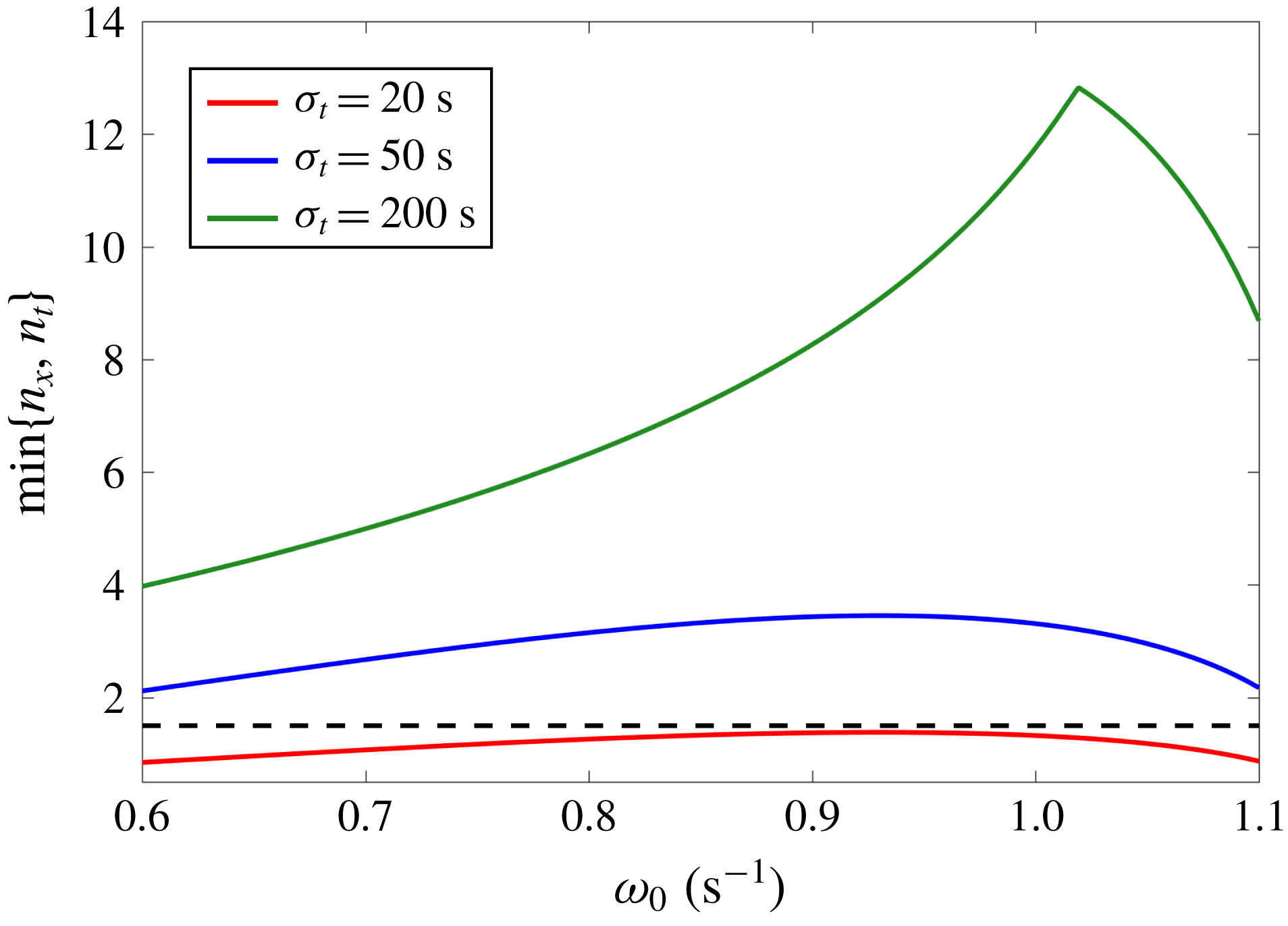
which is plotted in figure 11. The cusp in the plot at
 $\unicode[STIX]{x1D714}=\unicode[STIX]{x1D714}_{cusp}\simeq 1~\text{s}^{-1}$
for
 $\unicode[STIX]{x1D70E}_{t}=200~\text{s}$
exists because the curves for
 $n_{x}$
and
 $n_{t}$
intersect each other. For
 $\unicode[STIX]{x1D714}<\unicode[STIX]{x1D714}_{cusp}$
,
 $n_{x}$
is less than
 $n_{t}$
and vice versa for
 $\unicode[STIX]{x1D714}>\unicode[STIX]{x1D714}_{cusp}$
. It is clear that as the forcing time window increases,
 $\min \{n_{x},n_{t}\}$
increases since the value of
 $n_{t}$
increases even though
 $n_{x}$
remains the same. The value of
 $\min \{n_{x},n_{t}\}$
is less than 1.5 for
 $\unicode[STIX]{x1D70E}_{t}=20~\text{s}$
. According to the results in § 3.2, for any effects of interference to be evident, the minimum of
 $n_{x}$
and
 $n_{t}$
must be reasonably larger than 1. This explains why we do not observe any peaks or troughs in the variation of
 $\unicode[STIX]{x1D6E4}$
for
 $\unicode[STIX]{x1D70E}_{t}=20~\text{s}$
. It is to be noted that for the forcing parameters chosen, even if the spatial extent allows for multiple reflections to interfere, the temporal localization becomes the limiting factor for the case of smallest
 $\unicode[STIX]{x1D70E}_{t}$
.
5 Discussion and conclusion
5.1 Discussion on a geophysical application
In order to relate our studies to a geophysical scenario, we consider a specific example of the tropical cyclone Dora that happened from 27 January to 8 February 2007 (totally 11 days), which was at the same time as the Cirene research cruise (Vailard et al.
Reference Vailard, Duvel, McPhaden, Bouruet-Aubertot, Ward, Key, Bourras, Weller, Minnett and Weill2009). Cuypers et al. (Reference Cuypers, Le Vaillant, Bouruet-Aubertot, Vialard and McPhaden2013) analyse the data collected by the cruise for the near-inertial wave activity induced by the storm and provide estimates for the group velocity of the internal waves in the upper ocean (depths of 30–100 m). They find that the group velocity has the horizontal component
 $c_{gh}$
in the range
 $0.07{-}0.14~\text{m}~\text{s}^{-1}$
and vertical component
 $c_{gz}$
in the range
 $2{-}5~\text{m}~\text{day}^{-1}$
. As the pycnocline can potentially result in internal wave reflections, its depth below the mixed layer provides the length scale
 $L\simeq 80~\text{m}$
. Using these scales, we can estimate the characteristic scale
 $L^{\ast }=2Lc_{gh}/c_{gz}\simeq 193{-}968~\text{km}$
and the travel time
 $t^{\ast }=2L/c_{gz}\simeq 32{-}80~\text{days}$
. Given that the cyclone had a diameter of roughly 200 km and lasted for around 11 days, the ratios turn out to be
 $n_{x}\simeq 0.21{-}1.04$
and
 $n_{t}\simeq 0.14{-}0.34$
. Since
 $n_{x}\lesssim 1$
and
 $n_{t}<1$
, we conclude that interference effects did not play a role in the propagation of the internal waves excited by cyclone Dora. Thus, performing a harmonic analysis to study the transmission of internal waves would lead to incorrect results as the forcing from the cyclone is sufficiently localized.
5.2 Conclusion
We performed a study of the effect of spatiotemporal localization on the transmission and interference of internal waves in non-uniform stratifications. To explore this idea, we presented an idealized problem of a two-layer stratification system with a finite-width transition layer across which the buoyancy frequency changes continuously. This stratified fluid system was forced by a spatiotemporally localized forcing in the vertical velocity at the top boundary. In order to obtain internal wave field solutions, a theoretical model by Ghaemsaidi et al. (Reference Ghaemsaidi, Dosser, Rainville and Peacock2016a ) was extended to consider localized forcings with Fourier analysis. We utilized the model to perform a parametric study and analyse the effects of localization on internal wave interference.
A practical criterion to determine whether the effects of interference would be evident was developed. This criterion is dependent on several parameters such as the temporal and spatial size of the forcing, the depth and buoyancy frequency of the upper layer and the dominant frequency and wavenumber of the forcing. It essentially quantifies the number of interactions between the reflected waves and the forcing that the spatiotemporal size of the forcing can support. For a motivating example, it was shown that this criterion meaningfully determines the parametric regimes where transmission peaks or troughs due to constructive or destructive interference are expected, as compared to harmonic forcing.
We performed a supporting set of laboratory experiments. For a given stratification and a fixed spatial nature of the forcing, we performed experiments for three different values of the temporal size of the forcing over a range of forced frequencies. These experiments were in very good agreement with the theoretical predictions for the rescaled maximum vertical velocity amplitude denoted by
 $\unicode[STIX]{x1D6E4}$
. As expected, upon temporal delocalization of the forcing, peaks and troughs in
 $\unicode[STIX]{x1D6E4}$
were seen to get stronger, thus indicating a greater degree of constructive or destructive interference. For the experimental parameters, we revisited our practical criterion and showed that it correctly explains the experimental results as well.
Overall, this work demonstrates that the transmission of internal waves undergoing interference and potentially resonant forcing in non-uniform stratifications is highly dependent on how spatiotemporally localized the excitation is. This is relevant to scenarios such as the amount of energy a storm can transfer to the deep ocean through surface excitation of near-inertial waves (Alford et al. Reference Alford, MacKinnon, Simmons and Nash2016).
Acknowledgements
We thank P. Maurer, S. Ghaemsaidi, P. Odier, T. Dauxois and S. Joubaud for insightful discussions and guidance on numerical and experimental methods. We also thank A. Gallant for help with the experimental set-up and the three anonymous referees whose suggestions notably improved the manuscript. This work was partially supported by ONR Physical Oceanography Grant N000141612450 and NSF Physical Oceanography Grant 1357434.