Introduction
It is well known that both the material microstructure size and the model dimensional size in nanoscale systems have profound effects on material behavior. Investigating these size effects is important to tailor/upgrade material and design new materials. However, the model simulation may involve multiple physics and may need sufficiently large model size for its accuracy; thus, multiscale modeling and simulation is a must. In the last two decades, atomistically based multiscale analysis saw explosive development in methodology to meet the challenge in developing nanotechnology. Significant contributions on spatial quasistatic multiscale analysis include but are not limited to the FEAt method [Reference Kohlhoff, Gumbsch and Fischmeiser1], which is the first one combining atomistic analysis by molecular dynamics (MD) with continuum analysis by finite element (FE) methods, the quasicontinuum (QC) method [Reference Tadmor, Ortiz and Phillips2], the bridging domain method (BDM) [Reference Xiao and Belytschko3], the coupled atomistic/discrete dislocation (CADD) method [Reference Shilkrot, Miller and Curtin4], the atomistic-to-continuum (AtC) [Reference Wagner, Jones, Templeton and Parks5], the concurrent atomistic-continuum (CAC) method [Reference Chen6], the generalized particle (GP) dynamics method [Reference Fan7], and the embedded statistical coupling method (ESCM) [Reference Saether, Yamakov and Glaessgen8]. Following ESCM, approaches that directly link atoms and FE nodes in a one-to-one manner, or through a form of interpolation, will be referred to as direct coupling (DC) method, which covers almost most of existing multiscale analysis. Only the last two (i.e., the GP and ESCM) belong to the non-DC methods, which use statistical averaging over selected time interval and volume in atomic/particle subdomain (or neighbor link cell) to determine the FE nodal displacement [Reference Fan9].
The earliest progress in the temporal multiscale field is the well-known efforts by Voter and colleagues, namely, hyperdynamics [Reference Voter10], parallel replica dynamics [Reference Voter11], and temperature-accelerated dynamics (TAD) [Reference Sorensen and Voter12]. PRD was developed for systems that undergo infrequent events. PRD is a robust approach, because it makes no assumption regarding the types of events [Reference Petez-Unzueta and Beynon13]. Both Voter’s hyperdynamics and TAD exploit aspects of transition state theory (TST) and the latter also spawned other methods. Work by Zhu, Li, and co-workers [Reference Zhu, Li, Samanta, Leach and Gall14, Reference Zhu, Li, Samanta, Kim and Suresh15] has developed a modeling framework that computes the atomistic energy landscape and uses them within TST to develop analytic expressions for thermally activated processes. This method requires the identification of minimum energy paths (MEPs) that are traversed between pristine and defected states of the material, including the saddle point that characterizes the lowest energy barrier between these states. Further, the nudged-elastic band (NEB) method can be used for such purpose [Reference Fan9, Reference Hankelman and Johenson16, Reference Brenner17]. Because dislocations and heat conductions are essential components that influence properties of crystal materials and their modeling remains multiscale in nature, several models are developed to investigate this challenge problem [Reference Xu and Chen18].
Looking back to the development of multiscale analysis in the last two decades, one may see the following shortcomings: a lack of real applications. This view has been emphasized recently by Curtin and Miller [Reference Curtin and Miller19]. It said “Unfortunately, there has been a lack of real applications of these elegant and sophisticated methods….” Obviously, connecting currently existed largest atomic simulation to full engineering scales is a major challenge [Reference Brenner17]. It indicates that MD and atomistically based multiscale analysis cannot fully satisfy the requirement for many real problems. Thus, developing new simulation method to improve and speed up insertion of nanotechnologies is important.
For the limitation of model size and its related accuracy validation problems, Fan et al. [Reference Fan, Stewart and Xu20] have developed the XGP method (short for the extended GP multiscale method), and developed a continuum solution-based scheme to validate the simulation accuracy. These results are summarized here due to their importance.
Model dimension effects
As summarized by Fan et al. [Reference Fan, Stewart and Xu20], most existing atomistically based models have sizes L X and L Y around 100 × 100 nm, the smallest one of 3.53 × 3.53 nm has poor accuracy [Reference Fan and Yuen21] and the largest two with size around 1000 nm or larger has relatively high accuracy by Yamakov et al. [Reference Yamakov, Saether, Phillips and Glaessgen22, Reference Yamakov, Saether and Glaessgen23] Among the listed models, the work given by Dandekar and Shin is notable [Reference Dandekar and Shin24, Reference Dandekar and Shin25]. They used four basic model sizes, namely, 10 × 15 × 4, 20 × 30 × 8, 50 × 30 × 8, and 60 × 70 × 16 nm3, and obtained the corresponding Young’s modulus of 224.42, 188.66, 180.63, and 177.93 GPa, respectively. It merits note that the simulation-determined Young’s modulus corresponding to the smallest model size has a value, i.e., beyond the Hashin–Shtrikman bounds of 155–213 GPa. In addition, with a larger model, the Young’s modulus tends toward the experimental observation.
Method review of assessing simulation accuracy
So far, the most popular approach for accuracy identification in concurrent multiscale analysis is to compare the results with the fully atomistic simulation such as MD. Although this kind of verification is effective, shortcomings include the requirement for large computational spatial capacity and time if the model size is large. Because accuracy verification with classical continuum solutions has great potential to open new avenues, Fan et al. [Reference Fan, Stewart and Xu20] proposed a way to overcome the intrinsic difficulty to handle these two types of data: one being continuous for continuum physics and the other is discretized for atomistically based analysis. Then, they use classical continuum solution such as Rice’s two-parameter crack-tip solution and the elastic solution of a tensile bar with a hole under tensile loading to check the simulation accuracy.
Model dimension size effects and the critical model size concept
The difficulty frequently meets in investigating the model dimensional size effects is the need of new method for developing a large model. This issue is addressed in the work of Fan et al. [Reference Fan, Stewart and Xu20] by an extension of the GP method in which the FE nodes are connected with the outer most particles, but not directly with atoms as many DC-type modeling do. Thus, it can reduce artificial effects such as ghost force on the most interesting atomic regions to obtain more accurate solution such as crack-tip parameters. This way balances the simulation accuracy and the large model size effect by a sequential procedure: First, lamping atoms to different scale particles with the GP method (see section “A brief introduction of the GP method”) followed by the FEA to further reduce the degree of freedom (DOF). The accuracy of this method is confirmed by comparisons of simulation results with classic analytical solutions of a Model-I edge crack of iron under plane strain condition and a central cylindrical hole in a two-dimensional plate. Results show that there exists a problem-dependent critical model size, L CR, above which the extra model size may not be necessary under a given error tolerance and below which the simulation result may underestimate fracture parameters such as the crack-tip displacement, the range of the traction-separation (TS) curve, and the critical energy release rate G IC as well as the initiation strain for the crack-tip BCC to FCC phase transformation.
Although the proposed XGP and the proposed accuracy validation methods are significant, real engineering problems frequently involve multiple physics. How to simulate this kind of physical coupling problem is a challenge, which may need new simulation philosophy. The present work is an effort toward this direction to meet the above requirements. Specifically, a renewed methodology is proposed and exemplified by thermomechanical analysis of perlite steel consisted of alternatively arranged ferrite and cementite layer. This work emphasizes neither traditional point-to-point–based field analysis nor the nucleation and evolution of individual defects. What it emphasizes is the failure mechanism, control factors, and design criterion within the content of size effects. This article is organized as follows. Section “A brief introduction of the GP method” briefly introduces the GP method (remark: If one is interested in the XGP method, the paper [Reference Fan, Stewart and Xu20] should be referred to). Section “Failure problem of the alternatively-arranged ferrite and cementite layers with Bagaryatskii crystalline orientation” introduces the failure problem of pearlite and the complicated structure of the alternatively arranged ferrite and cementite layers with Bagaryatskii crystalline orientation. Section “‘New’ approach in nanoscale simulations” shows some new findings of size effects in thermomechanical coupling using the proposed “new” method in nanomechanics. Section “Derived results of size effects” gives the detail of the proposed new method and its application for thermomechanical coupling. This is followed by the section “Summary and conclusions”. The article ends in section “Methods,” which describes the detail of method in simulation.
A brief introduction of the GP method
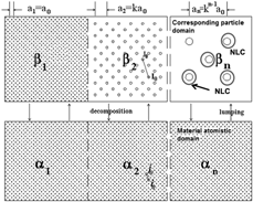
In most atomistically based multiscale modeling or the DC type methodology, the materials in both sides of scale interface are different. Atomistic field is nonlocal in which atoms subject to forces from other atoms within a finite distance. On the other hand, continuum is local in nature, where stress is directly determined only by the strain at that location. This inconsistent material constitutive property is the main reason for the observed artificial effects such as ghost forces at the interface (Shenoy et al. 1999). Although it can be partially reduced by the addition of the negative of these ghost forces as deadloads, the premise of this correction is the calculation of the ghost force first. This is not easy for many engineering problems involving complicated structure and various loading conditions. Furthermore, although using discrete FE nodes with interpolation function is a way to return the continuum assumption to the discrete media for the simulation, one may find other direct ways to do it. This is the philosophy underlying the GP methods. Specifically, the GP model consists of particle domains of different material resolution of βn (n = 1, 2, …, m) but with the same material structure such as body-centered cubic (bcc), face-centered cubic (fcc), and hexagonal close-packed (hcp). Here, scale n = 1 is the atomistic scale and n = m is the highest particle scale. Its basic concepts with its bottom-up lumping and top-down adaptive decomposition processes surrounding the so-called neighbor link cell (NLC) of each particle are illustrated in Fig. 1, where the GP concept of scale duality and structures invariance at all scales (n = 1, 2, …, m) are also schematically shown. The number of atoms ℓ n that one particle represents and the generalized particle lattice constant a n in the scale n can be calculated by [Reference Fan7]
 $${\ell _n} = {k^{3\left( {n - 1} \right)}}\quad ,$$
 $${a_n} = {k^{\left( {n - 1} \right)}}{a_0}\quad ,$$
where a 0 is the atomic lattice constant, k is the scale ratio of the generalized lattice constant of the adjacent scales (n + 1), and n (see top of Fig. 1). To see how effective the GP method is in reducing DOF, let us look at the following examples: When k = 3 for domain scale n = 3, 4, 5, each particle consists of 729, 19,683, 531,441 atoms, respectively, in average by Eq. (1), a huge DOF saving can thus be obtained. If one needs to further increase the model size for application, one may put FE nodes at the remotest boundary of the largest particle domain to greatly enlarge the distance between FE nodes and the most important atomistic field. As a result, the so-called XGP method can further substantially reduce the artificial effects, keeping the accuracy high while the model is with very large size. In addition, taking the advantage of particles as discrete as atoms, the GP calculations are conducted in the corresponding atomistic domain with an inversed-mapping method to get the correct potential and the force; thus, its algorithm is the same as MD and a lot of MD code can be used for the GP calculation. The basic principle for this mapping and inversed mapping is based on the Cauchy–Born rule [Reference Xiao and Belytschko3, Reference Fan9]. The accuracy of the GP method has been verified and its applications to several engineering problems such as dislocation nucleation and propagation, layer coating, and crack propagation were successful [Reference Fan7, Reference Fan9, Reference Fan, Stewart and Xu20, Reference Fan, He and Stewart26].
GP concept of scale duality and structures invariance at all scales (n = 1, 2, …, m) with n = 1 being the atomic scale. Domain βn is the corresponding particle domain to the atomistic domain αn (n = 1, …, m) of the material. The upward arrow denotes the αn to βn lumping process and the downward arrow denotes the adaptive inverse particle to atom decomposition process. (Reproduced from Ref. Reference Fan, Stewart and Xu20).

Failure problem of the alternatively arranged ferrite and cementite layers with Bagaryatskii crystalline orientation
Layered structure and its failure
The fundamental microstructure of pearlitic steel is alternatively arranged ferrite and cementite thin layers. The assembly of these layered structure forms many randomly orientated pearlitic colonies, which are the basic element of the steel. Because of this layered structure, pearlitic steel has superior mechanical properties in strength, ductility, wearability, fatigue, and so on [Reference Petez-Unzueta and Beynon13, Reference Langford27, Reference Clayton28, Reference Hodson and Preston29, Reference Sheng, Fan and Peng30], and there are many other extensive research works in developing experiments and theoretical analysis to show the failure of these layered material [Reference Gardner and Wilsdorf31, Reference Gardner and Wilsdorf32, Reference Park and Bernstein33, Reference Rosenfield, Votava and Hahn34, Reference Miller and Smith35]. Among these, the experimental observation by Langford [Reference Langford27] shows “there is no evidence for extensive, brittle fragmentation of cementite plates thinner than 0.01 mm” and “there is no evidence for gross plastic deformation of cementite plates thicker than 0.2 mm.” At the same time, phenomenological models were developed such as the one given by Bower and Johnson [Reference Bower and Johnson36] based on the nonlinear kinematic hardening model of Armstrong and Frederick [Reference Armstrong and Frederick37]. Although most models are phenomenological in nature, there are works based on continuum multiscale analysis. Specifically, an analysis across micro/meso/macroscopic scales was conducted by Fan et al. [Reference Fan, Gao and Zeng38] for investigating the cyclic behavior of pearlitic steel in which all scales are assumed to be continuum. The key to that multiscale analysis is to develop the constitutive laws for a unit cell at the mesoscale, which use self-consistent scheme linking to the macroscopic stress as well as linking to dislocations in the microscale through the dislocation pile-up theory of Eshelby et al. [Reference Eshelby, Frank and Nabbaro39] Although these works are significant, there are outstanding questions related to the mechanisms of microstructure–property relationship and failure. For instance, many works show that the yield stress of pearlite steel is inversely proportional to the interlaminar spacing but Modi et al [Reference Modi, Deshmukh, Mondal, Jha, Yegneswaran and Khaira40]. show below a critical spacing (=600 nm) of interlaminar layers the ultimate tensile strength and ductility remain constant due to residual stress. Furthermore, although the number of interfaces per volume or layer spacing was found to affect thermal stability substantially [Reference Zheng, Capenter, McCabe, Beryerlein and Mara41], experimental observations of those thermomechanical coupling is very difficult in measuring. This limitation of experiments makes atomistically based multiscale analysis an ideal method for evaluating the interface effects of these systems on thermomechanical coupling. Note that there are several works [Reference Guziewski, Coleman and Weinberger42, Reference Guziewski, Coleman and Weinberger43, Reference Guziewski, Coleman and Weinberger44] that investigate the important role of the interface between ferrite and cementite layers on mechanical behavior from the point of view of chemistry and energetics. In this work, however, we take the interface size effects as a key to investigate the thermal mechanical coupling and the possible failure mechanism.
Bagaryatskii crystal orientation
Although there is consensus that the cementite layers in pearlite can exhibit a single consistent orientation relationship (OR) with ferrous layers among the lamellae, three kinds of ORs are consistently reported [Reference Bagaryatskii, Nosova, Tagunova and Kristallicheskoi45, Reference Zhou and Sheflet46, Reference Zhang and Kelly47]. They are Bagarystskii OR, Isaichev OR, and Pitsch-Petch OR. Because Bagarystskii OR is the most commonly observed ORs, it will be the focus layer investigated in this work. Using the convention a < b < c of crystal lattice constants for the unit cell of cementite, Bagaryatskii orientation has crystalline relationship between cementite and ferrite of a lamellae as follows:
[100]Cementite ‖  ${\left[ {1\bar{1}0} \right]_{{\rm{Ferrite}}}}$, this direction determines the model X-axis.
[010]Cementite ‖ [111]Ferrite, this direction determines the model Y-axis.
[001]Cementite ‖  ${\left[ {11\bar{2}} \right]_{{\rm{Ferrite}}}}$, this direction determines the model Z-axis.
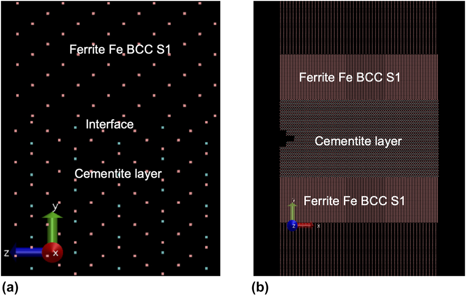
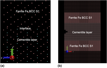
Here, symbol “‖” denotes two directions before and after “‖” are parallel. Their interface structures are shown in Fig. 2(a) (YZ plane) and Fig. 2(b) (XY plane).
The structures in ferrite and cementite layers and their interface in the Bagaryatskii OR showing (a) the (100) projection or along the YZ plane and (b) the (001) projection or along the XY plane. The symbol “Sx” denotes the scale of the domain, for instance, S1 represents the first scale and S2 is for the second scale of the particles.

“New” approach in nanoscale simulations
Observations of interesting phenomenon
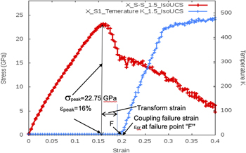
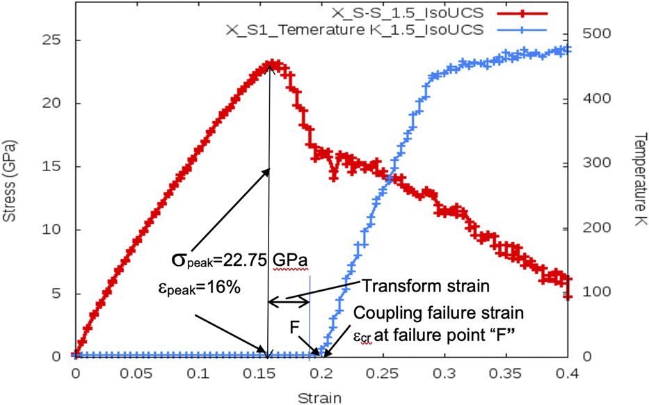
A GP model is designed and its atomistically based multiscale simulation is conducted at the temperature 2 K under transverse displacement loading along the X-direction. The model is subject to boundary displacement loading, controlled by the model box dimension. According to the boundary-constrained conditions, there are two kinds of simulations [Reference Pedone, Malavasi, Menziani, Segre and Cormack48]: one is called constrained simulation (CS), and the other is called UCS representing nonconstrained simulation. In the CS, the lateral boundaries are fixed but in the UCS, they are not. As an example, if the displacement loading is along the X-direction, the Y and Z box sides are fixed in the CS with the Poisson’s ratio being zero but in the UCS, the lateral displacement can be adjusted by a barostat to describe the Poisson’s effect. Figure 3 is obtained under the UCS-type simulation using Berendsen barostat to develop the lateral deformation. In Fig. 3, the left part shows the stress–strain curve in which the peak stress σpeak = 22.75 GPa occurs at the strain εpeak = 16%. The blue curve on the bottom and right part is the strain–temperature curve, which is flat on the bottom about 2 K and quickly raise to about 480 K after the point “F” at the so-called failure strain εcr = 19%. This curve is unexpected, which suggests the used thermostat cannot control the heat generation after that strain value as usual. This phenomenon may be called thermal instability. In fact, the MD simulation for the complicated temperature transient raising process at the point F is difficult, say, in using suitable thermodynamic ensemble. On the other hand, traditional methods in science with experiment-hypothesis-verification steps have proved historically success in solving many complicated problems. It may also be effective in material science for atomistically based simulation at nanoscale and mesoscale simulation, including coupling problems of different physics. Here, we use that method to try the analysis and call it as a “new” method or refreshed method, which will include the following stages: Observation → hypothesis → verification → derivation and application. In the following, this method will be exemplified by investigating size effects of above-mentioned thermomechanical coupling problems. Observations from Fig. 3 with the interesting phenomenon have been repeatably shown in several CS simulations under transverse loading along the X-axis (Figs. 4 and 6–8); thus in the next several sections, hypothesis will be given based on the first stage with these observations.
Distinguishing the mechanical strength σpeak = 22.75 GPa at peak strain εpeak = 16% from the coupling failure strain εcr = 20%. X denotes loading is along the X-axis, S–S is strain–strain curve, and “S1_Temperature” shows temperature at scale 1 domain. “1.5” is the separation distance (Å) between ferrite and cementite’s layers (see Effects of spacing size between cementite and ferrite layer on the mechanical strength σpeak and the critical coupling strain εcr). “isoUCS” indicates the UCS is conducted by isotropic barostat (see “Methods”).
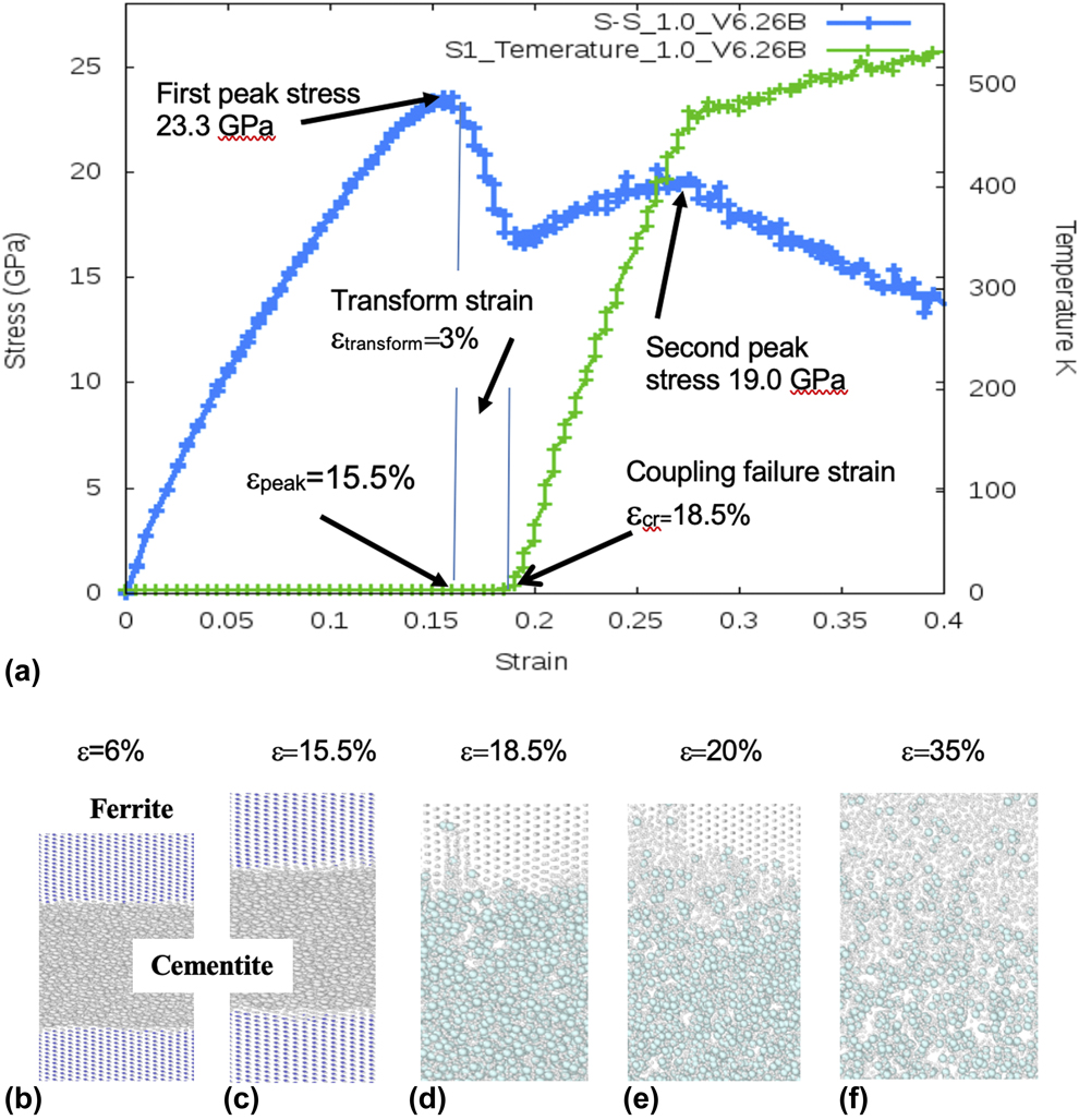
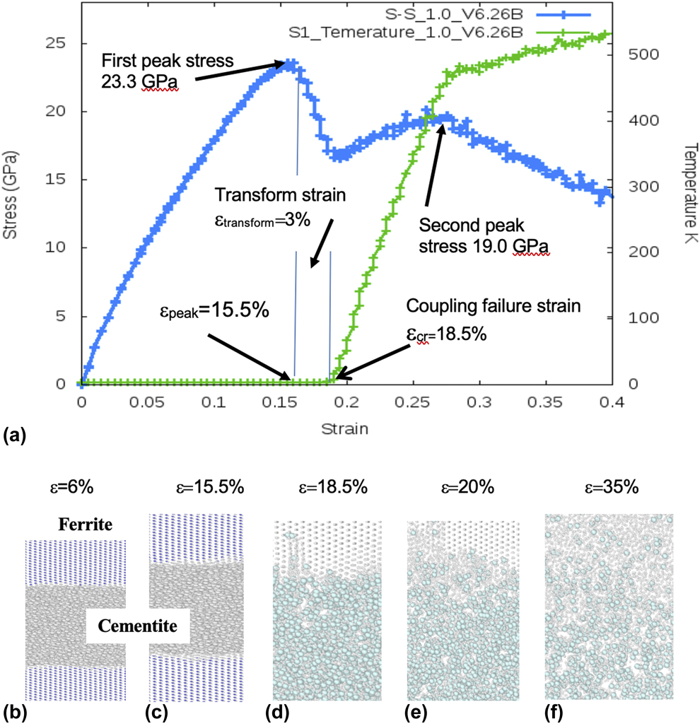
Correlation of material microstructure with applied strain in which (a) shows the global stress-strain and temperature-strain curves and (b–f) show how microstructures depend on strain values of (b) ε = 6%, (c) ε = 15.5%, (d) ε = 18.5%, (e) ε = 20%, and (f) ε = 35%. Note: microstructure-strain relationships depend also on where the temperature transition occurs. For the present case of coupling failure strain εcr = 18.5% and εpeak = 15.5%, (c) shows that the microstructure at the mechanical strength σpeak = 23.3 GPa keeps normal until after the addition of transformation strain 3% the failure starts with structure instability. In (a), “1.0” denotes that the spacing between ferrite and cementite layer is 1.0 Å. “V6.26” indicates the volume ratio of ferrite over cementite is 6.26, and “B” is the series number of the simulation. The simulation is with X-, Y-, and Z-periodic boundary conditions.
Hypothesis and its underlying mechanisms
Before the hypothesis is given, some physical background is introduced first. Thermomechanical coupling is a thermally activated process. It involves random atomic motion, diffusion, and defect nucleation/growth, which make the material ineffective and damaged; thus, the applied strain that starts a massive atomic random motion is defined as the initial failure point in this work. Note that this initial failure definition is intended to be conservative to make the structure safety highly guaranteed. In fact, structure failure in engineering usually involves failure of a large volume of materials but here involves only small volume in the very local region. It therefore cannot be directly used in the structure or failure criterion. Nevertheless, this definition gives a good threshold for failure initiation and a criterion for primary material design.
The general equation to describe these various random processes is the Arrhenius equation [Reference Shackelford49]. Following the work by Voter et al. [Reference Voter, Montalenti and Germann50] and Zhu et al. [Reference Zhu, Li, Samanta, Leach and Gall14, Reference Zhu, Li, Samanta, Kim and Suresh15], its temperature dependence of the transition rate, υ, with the TST can be expressed by the following form:
 $$\upsilon = {f_\upsilon }\exp \left( {{{ - Q\left( {\sigma ,\;T} \right)} / {{k_{\rm{B}}}T}}} \right)\quad ,$$
where f u is the system attempt frequency and k BT is thermal energy with k B as the Boltzmann constant. Q(σ, T) is the energy barrier, which is also called activation energy. The larger the value Q, the lower the transition rate υ, indicating that the defect (e.g., dislocation or voids) is hard to generate due to the large barrier Q. It is seen from Eq. (3) that the quantity Q is of central importance for the initiation of random processes or defects (e.g., voids and dislocations). In general, the activation energy Q(σ, T) is a function of temperature and applied stress. Zhu et al. [Reference Zhu, Li, Samanta, Leach and Gall14] assumed the following multiplication form with variable separation function for investigating the nucleation of dislocation:
 $$Q\left( {\sigma ,\;T} \right) = \left( {1 - {T / {{T_{\rm{m}}}}}} \right) \cdot {Q_0}\left( \sigma \right)\quad ,$$
where Q 0(σ) is the function of applied stress only and T m is the material melting temperature. Equation (4) satisfies two extreme conditions: when T = T m, there is no energy barrier and when T = 0, the activation energy equals Q 0(σ). This multiplication form is adopted here but will not take the linear temperature dependence for that part of activation energy. It turns out
 $$Q\left( {\sigma ,\;T} \right) = Q\left( {T,\;\sigma } \right) \cdot {Q_0}\left( \sigma \right)\quad ,$$
where Q 0(σ) is the function of stress only and Q(T, σ) is a decaying function of the temperature T. Here, we focus on effective domains and influence factors of the individual function but not their explicit mathematical expressions for each specific case such that the new method can be used more generally. The temperature transition point “F” in the strain axis distinguishes the contribution domain of the two functions. The applied strain before the strain point, F, contributes to the mechanical activation energy Q 0(σ) due to that it is conducted near 0 K temperature, and the thermal effects can be neglected. On the other hand, the corresponding variables after that strain point, F, contributes to Q(T, σ), which denotes the thermomechanical coupling activation energy. Now we give the hypothesis as following.
Hypothesis
Thermomechanical coupling activation energy is a fast decaying function of temperature such that after the temperature transition point, F, it reduces quickly to cause the energy barrier very low for massive atomic random motion and defects initiation and grow. As a consequence, the strain at the point “F” is defined to be the critical failure strain εcr, which is an index to show the failure initiation. Based on this terminology, the failure initiation criterion can be mathematically written as the following inequality:
 $${\varepsilon _{{\rm{total}}}} \ge {\varepsilon _{{\rm{cr}}}}\quad ,$$
where the total applied strain εtotal is an algebraic sum of εpeak and the transform strain εtransform (see Fig. 3 for the case εtransform is positive)
 $${\varepsilon _{{\rm{total}}}} = {\varepsilon _{{\rm{peak}}}} + {\varepsilon _{{\rm{transform}}}}\quad .$$
In other words, when the total applied strain εtotal reaches its threshold εcr, the system will suddenly start the failure process with initiation of atomic random motion and defects. Again, the critical failure strain, εcr, is the strain at the point “F,” where the temperature quickly increases from near 0 K to a high temperature (see Fig. 3). Now, a short discussion about this hypothesis is described as follows:
(i) This hypothesis is rational because any abrupt change of physical quantity will cause or relate to abnormal structural change. It will then start destroying the integrity/performance of the system, causing failure.
(ii) As emphasized in the previous description, the above proposed hypothesis is necessary and convenient for primary design due to that the existing thermodynamic NVT, NPT system, etc., are difficult to control the temperature in the transition process from constant temperature to the elevated temperature–dependent environment.
(iii) This hypothesis can be used for multiphysics, multilayers, multibehavior, and multi-intelligent system if they follow the Arrhenius equation. Thus, it may also be significant for couplings of electrothermal, electromechanical and electromagnetic, and biochemical of the layered structures. The difference between different systems is the source of the dissipative energy because different coupling systems have different types of dissipative energy, and in turn, it requires different coupling transformation variables and different explicit expressions of Eqs. (6) and (7).
(iv) Taking thermomechanical coupling as an example, the dissipative source can be internal/external frictions at the interface, which produces failure for pearlite layers. Because the frictional force is directly related to the size of the frictional area, thus the size of interface between different layers become one of the controlling factors for size effect on material behavior.
Verification
The key point for the verification is whether the prediction of the strain εcr at point “F” starts the random atomic motion to cause various defects in the microstructure. To confirm whether this is true, we use the GP multiscale method to obtain the underlying microstructure for each characterized strain ε. Different from Fig. 3 obtained by UCS-type loading, these works were conducted with transverse loading along the X-axis and with constrained boundary at the box boundary Y and Z. Several results are shown in Figs. 4(b)–4(f). Figure 4(b) shows microstructure under strain ε = 6%. In comparison with Fig. 2, it is clearly seen that both the structures of ferrite and cementite are basically the same as the original material with clearly separated cementite and ferrite domains. This type of microstructures remains unchanged even it reaches the mechanical strength σpeak = 23.3 GPa at the strain εpeak = 15.5%. When the total strain further reaches 18.5% by increasing the transformation strain by 3%, the microstructure pattern is seriously changed as shown in Fig. 4(d), where one can surprisingly see some of the cementite atoms move vertically to the ferrite layer and the moved atoms form voids in the local region of cementite layer. With further increase of strain, the distributed area of random structure expands as shown in Figs. 4(e) and 4(f) for strain 20 and 35%, correspondingly the voids in cementite layer are also randomly distributed, diffused, and coalesced to form large voids. It takes note that the strain 18.5% is at the transition point, F, from temperature 2 K to a high value. The result that calculated microstructure agrees well with the hypothesis, and Eqs. (6) and (7) indicate the prediction is true and the hypothesis is valid.
Here, we discuss two related questions. The first one is whether the strain of 35% is sufficiently large cause the local amorphous structure shown in Fig. 4(f). There are two sides to be emphasized for this question. One side is that the amorphous structure appears only in the local region but the strain is a domain average strain applied on the X-box boundary; it is not the highest strain in the local region. The same is true for the temperature and the true local temperature may be much larger than the averaged one. In other words, due to this and other reasons, this strain 35% and temperature 480 K may not be accurate for its local high value. The other side is that the whole model is only about 2–50 nm in dimension (see Methods) but the layer structure in pearlitic steel is more than mm or cm. Thus, using the observation result in that large scale to judge the phenomena in nanoscale is not fully accurate. Nevertheless, the conservative definition of the failure initiation and the approach proposed in this work offer an effective tool to analyze the size effects conveniently and effectively for multiple physics problems.
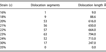
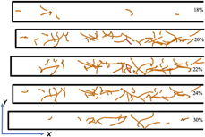
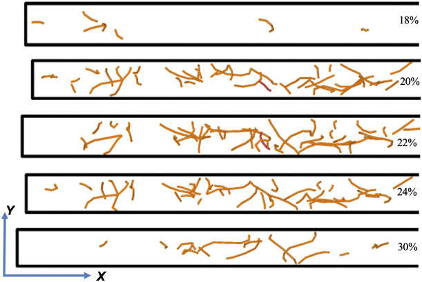
The second one is about the dislocation because it closely relates to the heat conduction and the failure process during thermomechanical coupling. Table I shows the dislocation segment numbers and the dislocation line length with respect to the applied strain in Fig. 3 under the UCS condition. These values and the dislocation patterns shown in Fig. 5 are obtained by the Open Visualization Tool (OVITO) [Reference Stukowski51]. For that case, dislocation initiated at strain 16% just after the peak stress σpeak = 22.75 GPa and the strain εpeak = 16%. The maximum segment number of 63 and the longest line length of 79.4 nm appear at strain 23%, about 3% after the failure initiation critical strain of εcr = 20% and then disappears at strain 35%. The result shows pure elastic behavior without dislocation and yielding before the peak stress. It also shows among various kinds of defects after the failure initiation dislocation takes important role. The typical dislocation pattern in the XY plane under the transverse loading for various strain is shown in Fig. 6, which shows dislocation patterns in the area about half of the dimension along the X-direction.
Dislocation variation with the applied strain.

Dislocation patterns at different strains for the UCS transverse loading. The strain values that causes the individual dislocation pattern are given on the right end of each figure and the related dislocation segment number and line lengths can be found in Table I. Note: The box shown here is about a half box, which is sufficiently to show the basic dislocation distribution for each case. In addition, if one takes the full box, the box will be short in the Y-direction such that the observation of dislocation pattern is difficult.
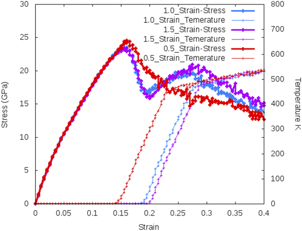
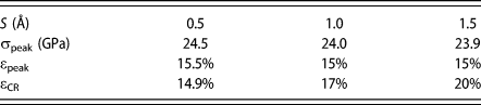
Effects of spacing size S between cementite and ferrite on the mechanical strength σpeak and the critical failure strain εcr.
Derived results of size effects
Based on the hypothesis, different results can be derived, which can then be used to further verify the hypothesis and open avenues for applications. Validation through lab physical test is difficult because of the small model size; a logical design of the idealized or imaginary verification test may be rational. An important but easily neglected problem is the size effects of the interface area between ferrite and cementite layers. In fact, this friction-related size effect is dominantly important because it is the source of dissipative energy, which causes temperature rising. In the following, this size effect will be investigated based on the “new” method and the proposed hypothesis.
Effects of spacing size between cementite and ferrite layer on the mechanical strength σpeak and the critical coupling strain εcr
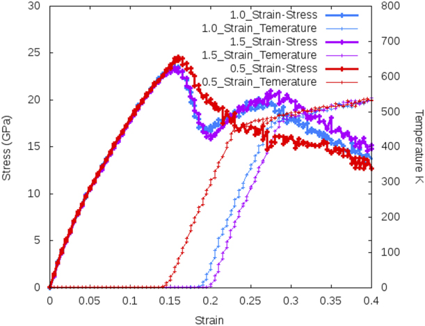
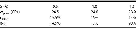
Here, the spacing size, S, is defined as the designed distance between the end of cementite layer and that of ferrite layer at the interface. The two-layered materials are mutually touched or overlapped under certain loading condition. The simulation result based on the “new” method is shown in Table II and Fig. 6. It is seen that the size effects of separation distance S between ferrite and cementite layer are very small on the value of peak stress σpeak and its corresponding strain εpeak. The former varies in the range of 23.4–24.5 GPa and the latter in the range of 15–15.5% for the spacing change from 0.5 to 1.0 Å and to 1.5 Å. These size effects related to pure mechanical loading as described in section “Hypothesis and its underlying mechanisms” are rational because the material structures to undertake various mechanical loading are almost the same when the temperature is near 0 K. It turns out that the mechanical strength for different layer separation does not change much. On the other hand, when the separation distance, S, changes in the same range from 0.5, 1.0, to 1.5 Å, the failure strain substantially increases from 14.9%, 17%, to 20%. In other words, the higher the spacing S, the larger the critical failure strain εcr. This completely different size effect is also rational because this change is related to the friction-produced heat generation by the thermomechanical coupling. The larger the spacing size S, the smaller the interface size. As a result, frictional area and frictional force will be smaller and the dissipative energy produced by the friction force will be smaller too. This will need to have more transformation strain to reduce more energy barrier such that the applied force or strain can drive the defect generation and reach the critical value εcr. The above rational result for both the pure mechanical- and thermomechanical coupling-produced size effect is a further validation for the hypothesis. Here, one can see the advantage of the hypothesis approach to replace the complicated simulation for the size effect. In fact, in this “new” method, one can get the quantitative size effects for primary designing the interface but does not need to involve the complicated determination of the true distribution of physical quantities and defects in the domain at room and/or elevated temperature.
Effects of separation distance S between ferrite and cementite layers on mechanical strength σpeak(εpeak) and failure strain εcr.
Thickness effects of cementite layer on the thermomechanical coupling under fixed volume ratio
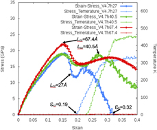
Here, the volume ratio is defined to be the ratio of ferrite volume V f over the cementite volume V C. Now, keeping the volume ratio V f/V c as a constant 4.7 but changes the size of the cementite layer along the Z-direction as 27, 40.4, and 67.4 Å to investigate these size effects on the mechanical strength σpeak(εpeak), failure initiation strain εcr, and the strain–stress curve. Figure 7 shows the results under the transverse loading along the X-axis. It is seen when the thickness L CZ of cementite is designed to be smaller, the peak stress becomes smaller. In addition, the coupling failure strain εcr and the total specimen fracture strain εF become smaller too. These results seem also to confirm the hypothesis-derived conjecture that internal frictional force at the interface between ferrite and cementite takes an important role in the thermal activation energy and critical strain εcr. The reason is that when the corresponding thickness, L CZ, of the cementite layer and the total dimension, L z, along the Z-direction decreases under the same boundary condition, the lateral compression strain near the interface will increase, and in turn, the frictional force will increase. On the other hand, when L CZ and L z become larger, then strain will be more evenly distributed to cause less constrained effects, which produces less frictional force and less change of the structure, thus it is harder for the material to fail.
Effects of cementite layer thickness L CZ or the model Z-dimension L z on the mechanical strength σpeak(εpeak), critical failure strain εcr, fracture strain εF, and the curve of thermal-mechanical coupling loading when layer separation S = 1 Å and volume ratio V is 4.7.
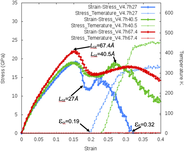
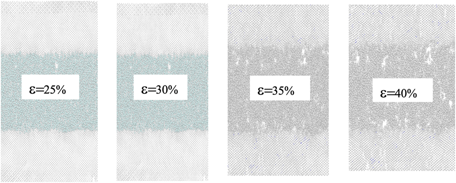
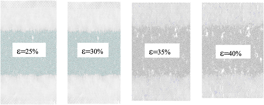
From Fig. 7 it is seen that there is a possibility for an idealized design to make the interface frictional force less than the driving force for void initiation to cause failure. This can be seen in the near bottom horizontal line with cementite thickness of 67.4 Å. This line is a temperature line but it is different from the corresponding line of cementite layer with thickness of 27 and 40.5 Å. For the latter two, the critical failure strain is 18.5% and 23% from which the layer structure will change, including cementite atoms that move to ferrite layer; voids are formed and then coalesced. To validate this conjecture, GP multiscale simulation was conducted. The material microstructure structures at strain 25%, 30%, 35%, and 40% are shown in Fig. 8. It is interesting that at all these high-value strains; the crystal structure in ferrite layers shown in the top and bottom parts of these models do not have any great change of crystallographic structure. Specifically, they cannot see the movement or diffusion of cementite atoms to the ferrite layer as shown in Figs. 5(d)–5(f). Although voids can be seen in the cementite layer, it is initiated within the cementite layer alone under high strain. This interesting result confirms the hypothesis-derived conjecture and makes the simulation for primary design of interface instructive and effective.
Microstructure versus applied strain for the optimum size of cementite layer.
Summary and conclusions
Intrinsic and extrinsic size effects of material microstructures on material failure are significant but can be complicated to get correct solutions. It needs a new approach. This work intends to use the traditional scientific methods with its key as “hypothesis” to deal with. Discussions and conclusions are given as follows.
(1) Recently, one pays attention to the solutions of size effects at the nanoscale with the hope to witness revolutionary discovery of their microstructure dependence on behavior for upgrading materials and designing new materials. However, the progress is limited so far, which makes developing nanoscale modeling with predictive capabilities essential. Nanoscale models are too small involving multiple physics, multiscales, confinement, high rates, etc. These make both the laboratory physical experiment and the near-realistic simulation of intrinsic and extrinsic size effects in materials complicated and difficult. For instance, effective thermodynamic ensembles are lacking for the transient process from constant temperature to higher and varying ones. As consequence, the simulation results may be insignificance or qualitatively inaccurate.
(2) Although there are different approaches to improve piece-by-piece the simulation methods, such as equilibration, loading pattern, thermostat, convergence, scale bridging, and data mining, a refreshed systematic scientific approach may be recalled. This “new” method is essentially the traditional scientific methodology, which has historically been proved to be very effective in scientific development by solving a lot of tough and long-lasting problems. Essentially, this method consists of the following four stages: observations, hypothesis, verifications, and applications for further validations. It takes notice that the main difference between the refreshed scientific method and the traditional one is that more computational work is used in almost all the four stages than the traditional ones. This difference is due to that the very small nanoscale model prohibits a lot of laboratory physical tests for observation and verification. On the other hand, validation by fully atomistic simulation needs very large and fast computers. This space and time limitation also prohibit one from using a large model for application. As a result, multiscale analysis will play more and more important role in the development of the “new” method.
(3) The four stages of the “new” method can be summarized as follows:
Observations
From a large amount of GP numerical simulation near zero temperature, one finds the strange phenomenon that the strain–temperature curve quickly increases its slope at a critical strain εcr as shown in Figs. 3, 4, and 6–8. This kind of phenomenon is anomaly and a special attention should be given to see whether it is rational.
Hypothesis
If directly explaining the observations is difficult, a hypothesis may be given. Certainly, this hypothesis must be based on physical principle or common accepted knowledge. Taking the hypothesis related to its thermomechanical coupling as an example, the energy barrier or activation energy Q(T, σ), which controls defect generation in an Arrhenius-type equation for defect generation, is assumed to consist of two parts. One is caused by pure mechanical loading characterized by peak stress σpeak and its corresponding strain εpeak when the simulation is conducted near 0 K. This low temperature simulation originally is to reduce the thermal noise, but now its function increases, which serves also as a great tool to separate the mechanical-type contribution to the total activation energy as shown in Eq. (5). This separation is rational because at near zero temperature, the thermal contribution is very small. Consequently, the second part characterized by the strain at or larger than the strain at the temperature transition point F represents the contributions to failure from the coupling of thermal and mechanical loading. Instead of the linear temperature dependence on energy barrier given by Zhu et al. (2008) for dislocation nucleation, this work assumes that the thermomechanical coupling activation energy Q(T, σ) is a fast decaying function of temperature such that after the temperature transition point, F, it reduces quickly. This assumption indicates after the point, F, the energy barrier is very low comparing to the currently increased driving force such that massive atomic random motion and defects initiation and growing are realistic and temperature increases quickly to offer the corresponding dissipative energy. These make the hypothesis that failure initiation starts at the temperature transition point, F, as well as the derived Eqs. (6) and (7) rational.
Verifications
If the hypothesis is valid then at the point of peak stress σpeak or the corresponding peak strain εpeak, the material structure should not be randomly distributed because there are no thermal effects for such a low temperature. On the other hand, the material microstructure should be randomly distributed after the temperature transition point F. Fortunately these predictions of the microstructure are proved to be true by the simulation results shown in Figs. 5(b)–5(f). Specifically, the microstructure at the peak stress did show the original crystalline structure and at the temperature transition point “F,” the microstructure did show the random atomic motion to produce voids and dislocations.
Applications and further validations
Extending applications are the goal in developing the “new” methods for nanotechnology. Inversely the application results can be used to further validate the hypothesis. The two tests, namely, “spacing size effects” and “cementite thickness effects” designed in section “Thickness effects of cementite layer on the thermomechanical coupling under fixed volume ratio” are applications of size effects of the pearlitic steel. It shows the important effects of interface structure such as the spacing and the layer thickness on the failure. The obtained results are consistent with physical principle that the small size (i.e., layer spacing and the layer thickness) will increase the internal frictional force. In turn, the friction produces more dissipative energy and transfer it to heat to initiate the atomic random motion; thus, the smaller the size, the lower the smaller the failure strain εcr. This rationality indirectly further validated the hypothesis and the “new method.” This may be important for nanotechnology because the friction-induced temperature is indeed a key in nanotechnology, which produces difficulties to the development of nano-micro system.
(4) This work is a preliminary work in using the “new” or refreshed scientific approach centered by “hypothesis” to solve size problem for multiple physics problems. Although this approach shows hope in convenience, effectiveness, and accuracy, lots of works need to be done. Future work includes carrying on reliable benchmark test to further verify its accuracy and to carry on different types of loading with different form, Q(T, σ), of thermomechanical activation energy to treat more complicated engineering problems.
Methods
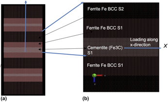
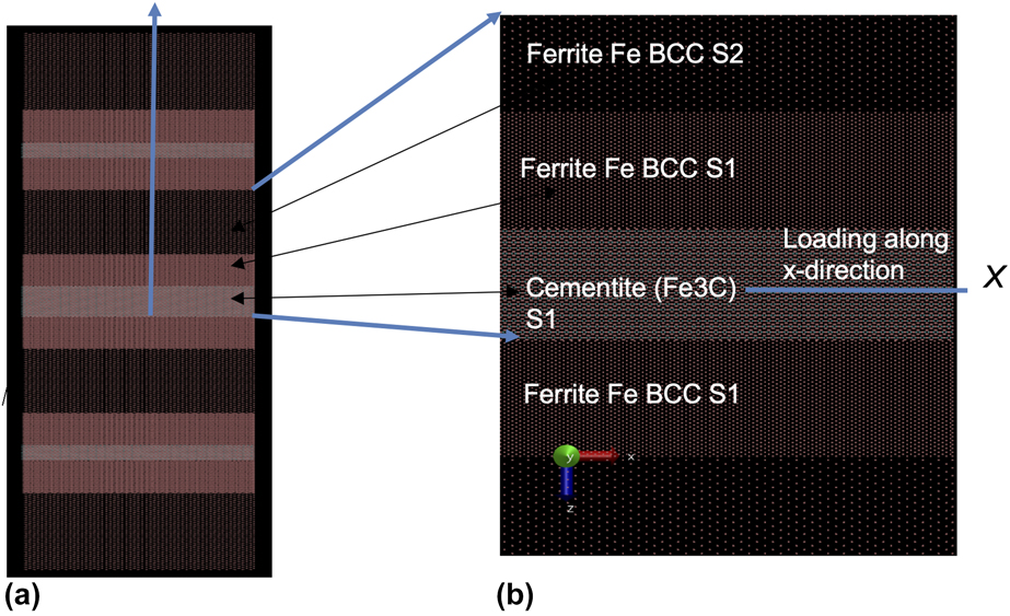
In the GP nanoscale simulations, the procedure is the same as MD. One sets the geometric model first, then chooses thermodynamics ensemble such as NPT and NVT, followed by choosing potential to calculate the interatomic force and then apply a house developed code PMAP (short for the particle-based multiscale program) directly for the simulation. The basic model size in this work is L x − L y − L z: 234 × 19.9 × 480 Å3. The model is designed as simple as possible from the aspect of multiscale analysis because the focus of this work is to illustrate the new approach for multiple physics. In addition, the multiscale analysis has been verified and applied in several articles (see section “A brief introduction of the GP method”). Specifically, the model is with two scales. Scale 1 consists of atoms in both cementite and ferrite layer denoted as cementite S1 and ferrite S1 [Fig. 9(b)]. The interface investigated is between these two atomistic layers and its structure is shown in Fig. 1(a). Scale 2 is only for ferrite, in which connection with scale 1 is through the overlapped imaginary region [Reference Fan7]. All the loading is transverse along the layer plane [Fig. 9(b)], but longitudinal loading perpendicular to the layer plane along the Y-axis [Fig. 9(a)] is also useful and will be the work in the next step. In the simulation, periodic boundary conditions in the X-, Y-, and Z-direction are used to avoid effects of surface tension and all simulation is under CS condition except for the first case shown in Fig. 3.
(a) A two-scale schematic of a GP model with alternatively arranged ferrite and cementite layers of pearlitic steel under the longitudinal loading of Y-direction. (b) Under the transverse loading of X-direction.
For normal displacement loading condition, the thermodynamic NPT or NVT ensemble is used, respectively, for the equilibration and loading process. Equilibration with conjugate gradient (CG) energy minimization of 50 ps is chosen. To reduce thermal noises, the simulation temperature is 2 K when attempting to characterize the deformation/failure mechanisms. Guziewski et al. used several types of interatomic potentials [Reference Guziewski, Coleman and Weinberger42, Reference Guziewski, Coleman and Weinberger43, Reference Guziewski, Coleman and Weinberger44], namely, the embedded atom methods (EAMs [Reference Dow and Baskis52]), modified embedded atom methods (MEAM [Reference Baskes53]), and Tersoff potential [Reference Tersoff54], for describing the interatomic forces of pearlitic steel and concluded that while each potential found different absolute values, the trend in interfacial energies between these was the same for the EAM, MEAM, and Tersoff. Due to the time effectiveness of the EAM, we adopt the Fe–C_HA.EAM potential [Reference Hepburn and Ackland55] with the format of LAMMPS fs type for the simulation. The strain rate is 2.5 × 10⁹/s.
Acknowledgments
Ross Stewart at Coring Inc. has developed and improved several computer codes for the particle-based multiscale analysis (PMAP), which is the main program of the GP methods and extensively used in this work. His significant and wide contributions are greatly appreciated.