Implications
Despite age at first lambing plays a key role on the reproductive performance of sheep flocks, its inclusion in genetic selection programs remains scarce. This research focused on the suitability of two different parameterizations for the genetic evaluation of this trait, as well as the magnitude and statistical relevance of both genetic and environmental sources of variation. Results suggested a remarkable advantage for survival analysis techniques in contrast to mixed linear models, and the estimated heritability (h2=0.114) encouraged the inclusion of age at first lambing as selection objective in sheep breeding programs.
Introduction
Cost of producing and maintaining breeding ewes can be high in the sheep industry. Indeed, ewe lifespan can be partitioned into two basic time stages, the costly raising period from birth to first lambing, and the subsequent ‘productive life’ until ewe disposal. Replacement ewes produce no output of economic relevance (other than wool in some breeds) until they reach sexual maturity and give birth for the first time. Within this context, the length of the time interval between birth and first lambing become of special relevance for profitability of sheep flocks worldwide. Studies about age at first lambing (AFL) are not particularly abundant in the scientific literature, although highly heterogeneous values have been reported for this trait; within-flock averages can fluctuate from less than a year of age (Gallivan et al., Reference Gallivan, Kemp, Berger and Young1993) to almost 23 months of age (Gabiña, Reference Gabiña1989).
As other lifetime traits in animal species, AFL has a skewed phenotypic distribution with evident over-representation of the right tail, thus discouraging its analysis under standard Gaussian-related mixed linear models (El-Saied et al., Reference El-Saied, de la Fuente, Carriedo and San Primitivo2005). Both the generalization of Gaussian models to non-symmetrical patterns and the implementation of non-linear models on the basis of skew parametric distributions have been suggested in previous studies (Varona et al., Reference Varona, Ibáñez-Escriche, Quintanilla, Noguera and Casellas2008; Casellas and Bach, Reference Casellas and Bach2012; García et al., Reference Garcia, Carvalheiro, Rosa, Valente and Albuquerque2014). The main objective of this research was to evaluate two main parameterizations for the analysis of AFL in the Ripollesa sheep breed, the skew-Gaussian mixed linear model (sGML, Sahu et al., Reference Sahu, Dey and Branco2003) and the piecewise Weibull proportional hazards model (Casellas, Reference Casellas2007). In addition, environmental and genetic sources of variation were characterized in order to provide guidelines to shepherds to optimize flock management and to decide whether AFL can be considered as a reliable selection objective in current breeding schemes or not.
Material and methods
Animal Care and Use Committee approval was not necessary for this study because analyses were performed on existing field data obtained under standard farm management from commercial breeders. Both productive and reproductive data were collected by the stockbreeders themselves and administrated by the Ripollesa Breed Society (Associació Nacional de Criadors d'Oví de Raça Ripollesa (ANCRI), Monells, Spain) within the context of its performance recording scheme.
Field data source
The Ripollesa is a medium-sized sheep breed (rams, 75 to 90 kg of live BW; ewes, 50 to 65 kg of BW) reared in north-east Spain and managed under semi-extensive conditions. This breed is a representative example of the meat-type sheep industry from the Mediterranean basin, the ‘pascual’-type lamb being its typical commercial product (22 to 24 kg of live BW at slaughter). Ripollesa individuals have dark brown or black marks on the head and legs, and white semi-fine wool with closed fleece (Esquivelzeta et al., 2011).
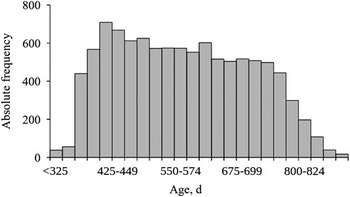
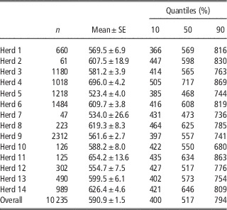
This research focused on the age at first lambing (AFL) defined as the number of days between the ewe’s birth date and the date of its first lambing. After discarding records shorter than 300 days and longer than 1000 days, AFL data from 10 235 Ripollesa ewes became available. These ewes were born between 1972 and 2013 in 14 purebred Ripollesa flocks with pedigree connection. All flocks located in the provinces of Girona and Barcelona (north-east Spain), they were active members of ANCRI, and contributed data to the official performance recording scheme; these data (e.g. ewe identification number, lambing date, lamb identification number, lamb sex and birth weight, among others) were registered by the shepherds themselves and further administrated by ANCRI. Within-flock summary statistics for AFL data are shown in Table 1, and Figure 1 illustrated the distribution pattern of raw AFL records. Note that all Ripollesa flocks were managed under continuous mating with several rams and, as usual in sheep flocks, ewe-lambs were kept apart from rams until they reached at least 4 to 5 months of age.
Histogram of age at first lambing data from the Ripollesa sheep breed.

Summary of the age at first lambing (days) data from the Ripollesa breed

The pedigree file included 12 399 individuals, 142 of them being rams contributing between one and 45 daughters each. Indeed, dam was known for all ewes with AFL data, whereas sire information was restricted to 984 ewes (9.6%). Given that several rams served at the same time, paternity information was recovered by genotyping replacement individuals for a custom 48-single nucleotide polymorphisms panel (Casellas et al., Reference Casellas, Fina, Bach and Piedrafita2014).
Bayesian models
Given the skewed distribution pattern of AFL data shown in Figure 1, analyses were performed on the basis of two different parameterizations characterized by Gaussian-related (Gianola and Fernando, Reference Gianola and Fernando1986) and proportional hazard-related (Ducrocq et al., Reference Ducrocq, Quaas, Pollak and Casella1988) hierarchical models (see below). Both approaches are able to fit data under unsymmetrical distributions, although the realized goodness of fit can differ substantially (Casellas and Bach, Reference Casellas and Bach2012). Without loss of generality, all analyses accounted for three independent sources of variation, that is systematic (b), permanent environmental (p), and additive genetic (a) effects. Vector b included season of birth of the ewe with four levels (winter, 34.9%; spring, 13.7%; summer, 15.0%; fall, 36.4%), birth type of the ewe with two levels (single, 58.1%; multiple, 41.9%), and birth weight of the ewe as a linear covariate (mean±SEM, 3.92±0.01 kg), whereas p accounted for appropriate flock-year-season effects with 120 levels.
sGML model
Sahu et al. (Reference Sahu, Dey and Branco2003) modified the standard Gaussian process in order to accommodate skew patterns by the inclusion of a single additional parameter (Λ). This extra parameter accounts for right- (Λ<0) and left-tail over-expression (Λ>0), as well as for symmetric Gaussian patterns (Λ=0). The following hierarchical structure was assumed to generalize the sGML model,
 $${\bf y}={\bf Xb}{\plus}{\bf Z}_{{\rm 1}} {\bf p}{\plus}{\bf Z}_{{\rm 2}} {\bf a}{\plus}{\bf e}$$
where y was the vector of phenotypic records, X, Z 1 and Z 2 were appropriate incidence matrices, and e was the residual term. The Bayesian implementation of this hierarchical structure was assumed as follows:
 $$\eqalignno{ & p({\bf b},{\bf p},{\bf a},\rsigma _{{\rm a}} ^{{\rm 2}} ,\rsigma _{{\rm p}} ^{{\rm 2}} _{,} \rsigma _{{\rm e}} ^{{\rm 2}} ,\Lambda ) \propto \ p({\bf y}\!\mid\!{\bf b},{\bf p},{\bf a},\rsigma _{{\rm e}} ^{{\rm 2}} ,\Lambda )\,\ p\left( {\bf b} \right)\,\ p({\bf p}\!\mid\!\rsigma _{{\rm p}} ^{{\rm 2}} )\ p(\rsigma _{{\rm p}} ^{{\rm 2}} ) \cr &\quad\quad\quad {\times}p({\bf a}\!\mid\!{\bf A},\rsigma _{{\rm a}} ^{{\rm 2}} )\,\ p(\rsigma _{{\rm a}} ^{{\rm 2}} )\,\ p(\rsigma _{{\rm e}} ^{{\rm 2}} )\ p(\Lambda ) $$
where σe 2 was the residual variance, σa 2 was the additive genetic variance, σp 2 was the permanent environmental variance, and A was the numerator relationship matrix (Wright, Reference Wright1922). Lack of sire information was accommodated into A by defining appropriate yearly within-flock genetic groups of unknown parents (Westell et al., Reference Westell, Quaas and Van Vleck1988). The p(y|b,p,a,σe 2,Λ) term was skew-Gaussian (Sahu et al., Reference Sahu, Dey and Branco2003; Varona et al., Reference Varona, Ibáñez-Escriche, Quintanilla, Noguera and Casellas2008),
 $$p({\bf y}\!\mid\!{\bf b},{\bf p},{\bf a},\sigma _{{\rm e}} ^{{\rm 2}} ,\iLambda )=\prod\limits_{i=1}^n {{2 \over {\sqrt {\rsigma _{e}^{2} {\plus}\iLambda ^{2} } }}\varphi \left( {{{e_{i} } \over {\sqrt {\rsigma _{e}^{2} {\plus}\iLambda ^{2} } }}} \right)\iPhi \left( {{\iLambda \over {\rsigma _{e} }}{{e_{i} } \over {\sqrt {\rsigma _{e}^{2} {\plus}\iLambda ^{2} } }}} \right)} ,$$
n is the number of phenotypic records in y, ϕ and Φ the density function and the distribution function of a standard normal distribution with kernel as defined between parentheses, respectively, and e i =y i –(x i b+z 1,i p+z 2,i a); note that x i , z 1,i and z 2,i were the ith rows of matrices X, Z 1 and Z 2, respectively. Priors for p and a were stated as p(p|σ p 2 )=MVN(0, I p σ p 2) and p(a|A,σ a 2)~MVN(0, A σ a 2), I p being an appropriate identity matrix with dimensions equal to the number of levels in p. Prior distributions for b, σ a 2, σ p 2, and σ e 2 were assumed scaled inverted χ 2 distributions with hyper-parameters ν=−2 and S 2=0. Following Varona et al. (Reference Varona, Ibáñez-Escriche, Quintanilla, Noguera and Casellas2008), p(Λ) was assumed improper uniform between −∞ and ∞.
Piecewise Weibull proportional hazards model (PWPH)
This model (PWPH) was adapted to the context of animal breeding by Casellas (Reference Casellas2007) on the basis of an original idea by Nguyen et al. (Reference Nguyen, Rogers and Walker1984) and Noura and Read (Reference Noura and Read1990). The parametrization relied on a standard Weibull model with parameters ρ and λ (Ducrocq et al., Reference Ducrocq, Quaas, Pollak and Casella1988), and included a time-dependent effect which changed in magnitude at given change points along the parametric space. Following the Bayesian development by Casellas (Reference Casellas2007),
 $$\eqalignno{ & p({\bf b},{\bf p},{\bf a},\rsigma _{{\rm a}} ^{{\rm 2}} ,\rsigma _{{\rm p}} ^{{\rm 2}} ,\rho ,\lambda ,\tau ,\xi )\ \propto \ p({\bf y}\!\mid\!{\bf b},{\bf p},{\bf a},\rho ,\lambda ,\tau ,\rxi )\,\ p\left( {\bf b} \right)\,\ p({\bf p}\!\mid\!\rsigma _{{\rm p}} ^{{\rm 2}} )\, \cr &\quad\quad\quad p(\rsigma _{{\rm p}} ^{{\rm 2}} ) \ {\times}\ \ p({\bf a}\!\mid\!{\bf A},\rsigma _{{\rm a}} ^{{\rm 2}} )\,\ p(\rsigma _{{\rm a}} ^{{\rm 2}} )\,\ p(\rho )\,\ p(\lambda )\,\ p(\tau )\,\ p(\rxi ) $$
τ was the vector of c change points (c⩾2) and ξ was the vector of c-1 regression parameters for the time-dependent effect. Focusing on the ith phenotypic record (y i ), its a priori distribution was stated as p(y i |b,p,a,ρ,λ, τ , ξ )=[h 0(t)β] [S 0(t) β ], where h 0(t)=λρ(λy i ) ρ-1 ξ к was the baseline hazard function derived from a piecewise Weibull density,
 $$S_{0} \left( t \right)=\,\exp\left\{ {{\minus}\left[ {\lambda ^{\rho } \xi _{k} \left( {y_{i}^{\rho } {\minus}\tau _{k}^{\rho } } \right){\plus}\mathop{\sum}\limits_{j=1}^{k{\minus}1} {\lambda ^{\rho } \xi _{j} \left( {\tau _{{j{\plus}1}}^{\rho } {\minus}\tau _{j}^{\rho } } \right)} } \right]} \right\}$$
was the piecewise baseline survival function with y i >τ k , and β=exp(x i b+z 1,i p+z 2,i a) was a scalar accounting for systematic, permanent and additive genetic effects. Following Damgaard and Korsgaard (Reference Damgaard and Korsgaard2006), improper uniform priors were assigned to ρ, λ, τ and ξ, whereas remaining a priori distributions were defined as for the sGML model.
Sampling from joint posterior distributions
Age at first lambing data were independently analyzed under models sGML and PWPH. Moreover, the number of change points of the Weibull baseline function must be chosen in advance for PWPH model and thus, seven independent analyses were performed from c=2 to c=8 (PWPH2 to PWPH8). All the unknown parameter in models were sampled from their marginal posterior distributions by appropriate Gibbs sampling (Gelfand and Smith, Reference Gelfand and Smith1990) or Metropolis-Hastings (Metropolis et al., Reference Metropolis, Rosenbluth, Rosenbluth, Teller and Teller1953). Three independent Monte Carlo Markov chains (MCMC) with 1 000 000 iterations were run for each analysis, and the first 100 000 iterations were discarded as burn-in. The suitability of the length of the burn-in period was evaluated by both visual inspection and the method of Raftery and Lewis (Reference Raftery and Lewis1992) on the sampling path of σ a 2. A total of 18 000 samples of model parameters were saved from each chain with a lag interval of 50 iterations. All analyses were performed in a server with two Intel® Xeon® E5-2400 processors with a CentOS 6.6 Linux operating system. In terms of central processing unit (CPU) time, models sGML and PWPH2 spent less than eight hours for each independent 1 000 000-iteration MCMC. Computing demand rose for models PWPH3 (~18 h) to PWPH8 (~52 h) as the number of change points increased.
Model comparison
The two parameterizations implemented in this manuscript (sGML and PWPH models) where compared by means of the deviance information criterion (DIC; Spiegelhalter et al., Reference Spiegelhalter, Best, Carlin and van der Linder2002). Note that DIC measures two different sources of model performance in terms of the posterior expectation of the Bayesian deviance (model fit) and the effective number of parameters (model complexity). This statistic can be computed from each MCMC and allows for a straightforward comparison between models where smaller DIC values indicate a better fit and a lesser degree of model complexity. Differences of at least three to five DIC units are generally considered as statistically relevant (Spiegelhalter et al., Reference Spiegelhalter, Best, Carlin and van der Linder2002). On the other hand, inference on predicted breeding values should play a key role for genetic selection programs. Within this context, Pearson's correlation coefficients between modal estimates of predicted breeding values from different model parameterizations were calculated at the end of the MCMC process.
Results and discussion
Age at first lambing in the Ripollesa breed
Our analyses focused on 14 purebred Ripollesa flocks and 10 235 ewes that averaged 591 days at first lambing, and within-flock averages ranged from 523 days to 696 days. These averages were free from upward biases due to infertile ewes (i.e. ewes incapable of getting pregnant that joined the flock until detected and culled by the shepherd) because only ewes with at least one registered lambing contributed phenotypic data, and censored records (Cox, Reference Cox1972) were not considered. This must not be viewed as a limitation of the parameterizations used in this research (both PWPH (Casellas, Reference Casellas2007) and sGML models (Guo et al., 2001) accommodate right-censored data) but an effort to guarantee field data quality. Age at first lambing in the Ripollesa breed seemed to be placed at the upper boundary of this reproductive trait, although the removal of all right-censored AFL records (i.e. ewes culled before their first lambing) may have biased downwards the average AFL in the Ripollesa breed. Nevertheless, less than 200 ewes were removed from the data set because they were culled at an age of two or more years and without lambing records. Other populations provided similar performances such as the Rasa Aragonesa (528 days to 688 days; Gabiña, Reference Gabiña1989) and the Churra breed (604 days; El-Saied et al., Reference El-Saied, de la Fuente, Carriedo and San Primitivo2005), which are also autochtonous breeds from Spain, the Yankasa breed from Nigeria (533 days; Osuhor et al., Reference Osuhor, Osinowo, Nwagu, Dennar and Abdullahi-Adee1997), or the Awassi breed reared in Spanish farms (~550 days; de la Fuente et al., Reference de la Fuente, Gabiña, Carolino and Ugarte2006). Nevertheless, age at first lambing in the Ripollesa breed was clearly delayed when compared with other dairy sheep breeds reared in Spain like Assaf (~450 days), Churra (~420 days; de la Fuente et al., Reference de la Fuente, Gabiña, Carolino and Ugarte2006) and Lacaune (433 days; Hernandez et al., Reference Hernandez, Elvira, Gonzalez-Martin, Gonzalez-Bulnes and Astiz2011). Smaller ages at first lambing were also reported in Finnish Landrace×Targhee (377 days) and Romanov×Targhee (365 days) flocks (Gallivan et al., Reference Gallivan, Kemp, Berger and Young1993). As a whole, these estimates for age at first lambing revealed a large scope for AFL improvement in the Ripollesa sheep breed.
Although the average of AFL data gave us an idea about the onset of the reproductive activity in the Ripollesa breed in a broad sense, both the histogram shown in Figure 1 and flock-by-flock specific data about more extreme quantiles (10% and 90%; Table 1) provided a more detailed characterization of the phenotypic dispersion pattern of AFL. Modal estimate (411 days; Figure 1) was clearly smaller than average estimate in all flocks, this leading to the overextension of the right-tail of the AFL distribution. The absolute frequency for AFL slowly decreased after the modal peak and until ewe-lambs aged ~2 years, showing an accentuated decline after that. The low incidence of first lambing from 2-year-old ewes (or even older individuals; Figure 1) could be linked with the preferential culling of ewes that failed to give birth by first time at these ages. As a whole, this depicted an atypical and non-Gaussian distribution patterns that must be properly accounted for by the analytical model.
Comparison between competing models
Deviance information criterion estimates regarding both Gaussian-related and proportional hazard-related parameterizations for the analysis of the AFL data are shown in Table 2. Although model sGML provided a more flexible framework when both positive and negative asymmetry in the data must be accommodated (i.e. over-expression of the right and left tail of the distribution, respectively), model PWPH was favored. Analyses did not support model sGML with an average DIC of 200 059 units when compared with PWPH models (<136 000 units); model fit under linear mixed model parametrizations was even worse when restricting the analysis to scenarios under perfect symmetry (L=0; DIC=245 703), although this could be anticipated given the modal and highest posterior density region at 95% (HPD95) obtained for L under model sGML (Table 3). Our estimates about goodness of fit suggested that linear models must be ruled out from AFL data analysis, whereas PWPH models were an appealing alternative with preferable statistical performances. This conclusion agreed with previous studies that advocated the superiority of survival analysis techniques when handling time interval data such as lambing interval in sheep (Casellas et al., Reference Casellas and Bach2012), age at first calving (García et al., Reference Garcia, Carvalheiro, Rosa, Valente and Albuquerque2014), or fertility- and longevity-related traits in cattle (Caraviello et al., Reference Caraviello, Weigel and Gianola2004; Schneider et al., Reference Schneider, Strandberg, Ducrocq and Roth2005, Reference Schneider, Strandberg, Ducrocq and Roth2006; MacNeil and Vukasinovic, Reference MacNeil and Vukasinovic2011). Within this context, the implementation of proportional hazards models seems a reasonable alternative for AFL data. To the best of our knowledge, this methodological approach had not been previously implemented for the analysis of birth-to-first parturition data in sheep, whereas few studies were performed in other ruminant species (Garcia et al., Reference Garcia, Carvalheiro, Rosa, Valente and Albuquerque2014).
Deviance information criterion (Spiegelhalter et al., Reference Spiegelhalter, Best, Carlin and van der Linder2002) for age at first lambing in the Ripollesa sheep breed under a skew-Gaussian mixed linear model (sGML) and piecewise Weibull hazard model with i change points in the baseline function (PWPHi)

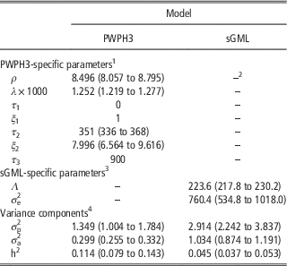
Mode (highest posterior density region at 95%) for model-specific parameters and variance components from the analysis of age at first lambing in the Ripollesa sheep breed under a skew-Gaussian mixed linear model (sGML) and a piecewise Weibull proportional hazard model with three cut points (PWPH3)

1 The baseline function was modeled within the context of a Weibull density with appropriate shape (ρ) and scale parameters (λ). Moreover, additional flexibility was gained by including a time-dependent effect defined between τ 1=0 and τ 3=900, and with magnitude ξ 1=1 and ξ 2 that changes at τ 2.
2 Not applicable.
3 The Gaussian mixed linear model included an extra parameter to accommodate skew-distributed residuals (Λ); note that σ e 2 was the residual variance.
4 Under model PWPH3, heritability (h2) was calculated on the original scale by applying h2=σ a 2/(σ a 2+σ p 2+1) as described by Yazdi et al. (Reference Yazdi, Visscher, Ducrocq and Thompson2002). On the other hand, the formula h2=σ a 2/[σ a 2+σ p 2+σ e 2+Λ 2(1–2/π)] can be applied to the sGML model (Sahu et al., Reference Sahu, Dey and Branco2003; Varona et al., Reference Varona, Ibáñez-Escriche, Quintanilla, Noguera and Casellas2008).
Focusing on PWPH parameterizations, model PWPH3 reached the smallest DIC estimate (Table 2), this being almost 1700 DIC units smaller than the following model (PWPH2). Moreover, models PWPH4 to PWPH8 revealed a progressive increase of DIC estimates, adding on average 262 DIC units for each extra change point in the model. This progressive penalization of more parameterized models suggested that marginal benefits of additional change points did not counterbalance model over-parameterization, and PWPH3 was a more parsimonious choice for AFL data from the Ripollesa breed.
Capturing skewness from AFL data
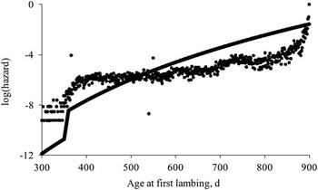
Both sGML and PWPH3 parameterizations evidenced the right-tail over-expressed distribution of AFL data in the Ripollesa sheep breed (Figure 1). Whereas sGML model provided a positive modal estimate of the skewness parameter (Λ) with its HPD95 clearly discarding the null estimate (217.8 to 230.2; Table 3), model PWPH3 smoothened out the slope of the Weibull baseline function after 351 days of age (HPD95, 336 to 368). This accommodated the rapid accumulation of ewes lambing short before their first birthday (Figure 1), accentuating the slope of the Weibull distribution characterized by the initial ρ and λ parameters; note that the magnitude of the time-dependent effect (ξ) on the baseline function raised from 1 (t⩽τ 2) to 7.996 (τ 2<t), and larger estimates from survival analysis must be interpreted as an increased risk of failure or, in our case, a higher probability of lambing in short. A graphical representation of the hazard function is shown in Figure 2 and compared with the non-parametric Kaplan–Meier estimate (Kaplan and Meier, Reference Kaplan and Meier1958). Note that both approaches provide similar estimates and departures must be partially attributable to the absence of systematic, permanent and genetic factors when computing the baseline hazard function under model PWPH3; the Kaplan–Meier estimate is computed from raw AFL data and all additional sources of variation are implicitly included. The need for this kind of additional modeling of the standard Weibull baseline function has been previously demonstrated on longevity (Tarrés et al., Reference Tarrés, Casellas and Piedrafita2005; Casellas et al., Reference Casellas, Varona, Ibáñez-Escriche, Quintanilla and Noguera2008) and fertility data (Casellas and Bach, Reference Casellas and Bach2012), although this should not be viewed as a weakness of the survival analysis techniques but a remarkable advantage in terms of flexibility of the PWPH (Casellas, Reference Casellas2007) model.
Logarithm of the hazard computed under modal estimates of baseline parameters from model PHPW3 (solid line) and the non-parametric Kaplan–Meier approach (Kaplan and Meier, Reference Kaplan and Meier1958; black dots).

Systematic and genetic influences on AFL
Although three systematic effects were included in the analytical model, only the season of birth of the ewe had relevant influences on the AFL under PWPH3 parameterization. Both birth type (single or multiple) and birth weight provided close-to-zero regression coefficients with their HPD95 clearly including the null estimate. This agreed with previous analyses in the Yankasa breed of sheep from Nigeria (Osuhor et al., Reference Osuhor, Osinowo, Nwagu, Dennar and Abdullahi-Adee1997), where the same systematic effects were also discarded. Focusing on the season of birth, spring-born ewes showed the longest AFL although regression coefficient for winter-born ewes did not differ (β=0.074; HPD95=−0.028 to 0.164) from spring-born ewes (this was fixed to 0 as reference). Summer- (β=0.159; HPD95=0.060 to 0.242) and fall-born ewes (β=0.394; HPD95=0.280 to 0.513) were more predisposed to shorter AFL. These estimates agreed with the pattern shown by the raw averages of AFL data from our data set for winter- (590±2 days), spring- (627±2 days), summer- (586±2 days) and fall-born ewes (580±2 days). It could be suggested that spring- and winter-born ewes were slightly penalized in terms of AFL because they were expected to give birth as a first time at counter-season; summer- and fall-born ewes-lambs took advantage of the natural breeding season, this providing better reproductive performances in terms of AFL.
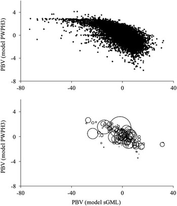
Models sGML and PWPH also showed remarkable departures from each other when capturing genetic and environmental random sources of variation. Whereas the mixed linear parameterization suggested that flock-year-season variance was almost three time that of the additive genetic variance, model PWPH provided even larger differences with a modal estimates of 0.299 for the additive genetic variance and 1.394 for the flock-year-season variance (Table 3). Heritability estimates from both parameterizations differed, this being clearly larger from PWPH3 (h2=0.114) than from sGML (h2=0.045). Unfortunately, there is shortage of heritability estimates for AFL in sheep in the scientific literature, and our estimate from the sGML model was slightly higher than the one obtained by Lôbo et al. (Reference Lôbo, Lôbo, Paiva, de Oliveira and Falcó2009) in a multibreed population (h2=0.04). Nevertheless, heritabilities form linear and proportional hazard models cannot be comparable at all. The advantage of proportional hazard models when capturing additive genetic variance from time-interval traits was previously reported by Caraviello et al. (Reference Caraviello, Weigel and Gianola2004) in dairy cattle and Casellas and Bach (Reference Casellas and Bach2012) in sheep, this potentially leading to more rapid genetic progress (Korsgaard et al., Reference Korsgaard, Andersen and Jensen2002). It is important to note that predicted breeding values from mixed linear and proportional hazard models cannot be directly compared because they are diametrically opposed. Shorter AFL intervals must be obtained by selecting those individuals with large and positive (model sGML) or large and negative (model PWPH3) predicted breeding values. Moreover, their magnitude can also differ because the sGML model assumes an additive structure for systematic and random effects (Sahu et al., Reference Sahu, Dey and Branco2003), whereas PHPW models rely on an exponential parameterization (Cox, Reference Cox1972). Within the context of the Ripollesa data set, departures in terms of predicted breeding values from sGML and PWPH3 are shown in Figure 3; as expected, the plot suggests a negative correlation of −0.636, even higher if only sires were considered (−0.694), and departures increased for genetic background predisposing to longer AFL. Within this context, differences between sGML and PWPH3 models in terms of response to selection must be larger if selecting for longer AFL than for shorter AFL. Although fertility-related traits have been historically considered as barely heritable (Fogarty, Reference Fogarty1995), the heritability under model PWPH3 endorses AFL as a candidate trait for current selection programs in sheep.
Plot of predicted breeding values (PBV) by the skew-Gaussian mixed linear model (sGML; x-axis) against PBV by piecewise Weibull proportional hazard model with three cut points in the baseline function (PWPH3) for all animals (upper panel) and sires (lower panel; the diameter of each spot characterized the number of evaluated daughters, from 1 to 45).

Acknowledgments
The author is indebted to the Ripollesa breed society (Associació Nacional de Criadors d'Oví de Raça Ripollesa, Monells, Spain) for contributing field data. The research contract of J. Casellas was partially financed by Spain’s Ministerio de Ciencia e Innovación (program Ramón y Cajal, reference RYC-2009-04049).