1 Introduction
Vertically distributed turbulent plumes, plumes in which the buoyancy source is distributed over some vertical distance
 $H$
, are ubiquitous in environmental fluid mechanics and occur over a very wide range of scales. Examples include thermal plumes that form around a standing person (Craven & Settles Reference Craven and Settles2006), melt plumes from icebergs (Wells & Worster Reference Wells and Worster2011; Kerr & McConnochie Reference Kerr and McConnochie2015) and thermal plumes that form next to a wall heated by the sun (Chen, Li & Mahoney Reference Chen, Li and Mahoney2001). Much prior research has focused on quantifying the rate of heat transfer from a vertical solid surface immersed in a fluid of different temperature such as a hot plate in air. Typically the heat flux is quantified in terms of a non-dimensional heat transfer coefficient (Nusselt number) correlated with the Rayleigh and Prandtl numbers, where the three non-dimensional parameters are given by
 $$\begin{eqnarray}Nu=\frac{hH}{k},\quad Ra=\frac{g^{\prime }H^{3}}{D\unicode[STIX]{x1D708}}\quad \text{and}\quad Pr=\frac{\unicode[STIX]{x1D708}}{D},\end{eqnarray}$$
respectively, where
 $h$
is a heat transfer coefficient,
 $H$
is the plate height,
 $k$
is the thermal conductivity of the fluid,
 $D$
is the fluid thermal diffusivity,
 $\unicode[STIX]{x1D708}$
is the fluid kinematic viscosity and
 $$\begin{eqnarray}g^{\prime }=g\frac{{\unicode[STIX]{x1D70C}_{a}-\unicode[STIX]{x1D70C}}_{W}}{\unicode[STIX]{x1D70C}_{a}}\end{eqnarray}$$
is the reduced gravity of the fluid at the wall relative to the ambient fluid, in which
 $\unicode[STIX]{x1D70C}_{a}$
is the ambient fluid density and
 $\unicode[STIX]{x1D70C}_{W}$
is the density of the fluid at the plate surface. The heat flux over the entire vertical wall is
 $P$
, given by
 $$\begin{eqnarray}P=hA\unicode[STIX]{x1D6FF}T,\end{eqnarray}$$
where
 $A$
is the plate area and
 $\unicode[STIX]{x1D6FF}T$
is the temperature difference between the plate and the ambient fluid. The Nusselt number
 $Nu$
is usually expressed in terms of powers of
 $Ra$
and
 $Pr$
. Different correlations are used depending on whether the natural convection boundary layer is laminar or turbulent, with the flow transitioning to turbulence at around
 $Ra=10^{9}$
– see for example Cengel & Ghajar (Reference Cengel and Ghajar2015), or other introductory heat transfer textbooks. Typically this work has focused on industrial-scale flows with application to, for example, cooling of electronics and refrigeration, though geophysical-scale flows have also been examined (Wells & Worster Reference Wells and Worster2008; Kerr & McConnochie Reference Kerr and McConnochie2015).
This approach has largely focused on heat (or mass) transfer rather than on the details of the wall plume flow induced by the buoyancy force (though it is this flow that drives the convective heat transfer so flow information is implicit in the Nusselt number correlations). Recent research into air flows in buildings has, however, focused on the induced plume flow, assuming that the heat flux is known (Chen et al. Reference Chen, Li and Mahoney2001; Cooper & Hunt Reference Cooper and Hunt2010 (CH); McConnochie & Kerr Reference McConnochie and Kerr2016 (MK); Bonnebaigt, Caulfield & Linden Reference Bonnebaigt, Caulfield and Linden2018 (BCL)). These papers, along with a similar paper by Gladstone & Woods (Reference Gladstone and Woods2014) (GW) that focused on a vertical line source rather than a vertical planar source, have used the plume theory of Morton, Taylor & Turner (Reference Morton, Taylor and Turner1956) to model the variation of volume flux and buoyancy in the plume as it develops vertically. This model is then used to examine the stratification that forms within an enclosure containing the plume using filling-box-type models (Baines & Turner Reference Baines and Turner1969).
One challenge to this approach is that it is very difficult to achieve a fully turbulent natural convection thermal boundary layer at laboratory scale. For example, an experiment run with a vertical flat plate immersed in water that is
 $50\,^{\circ }\text{C}$
hotter than the surrounding water will develop a thermal boundary layer that becomes turbulent approximately 14 cm from the base of the plate. Doubling the temperature difference (while avoiding boiling) only reduces this transition height to 11 cm. This height is often similar in order to the height of the experimental apparatus. For example, in the thermal experiments of Caudwell, Flór & Negretti (Reference Caudwell, Flór and Negretti2016), the wall thermal plume was laminar in the lower 20 cm of a 55 cm tank.
To overcome this problem, experimentalists working on air flows in buildings often use salt plumes (e.g. Linden, Lane-Serff & Smeed Reference Linden, Lane-Serff and Smeed1990). This has a number of advantages, including improved control over source and boundary conditions, significantly lower diffusivity
 $D$
, and the ability to create much larger density differences. For example, using a 10 % density difference salt solution will generate a buoyant boundary layer that is turbulent approximately 1 cm from the base of the plume. Therefore, using salt solution for the buoyancy source allows experimentalists to run experiments that are fully turbulent over a much greater percentage of the test rig height. Further, because buoyant fluid is forced into the plume through the wall source in the form of small horizontal jets, the flow is likely to trip to turbulence more easily and remain turbulent, as observed with round plumes that will remain turbulent over their whole height with source Reynolds numbers as low as 300 when tripped near the source (Huppert et al.
Reference Huppert, Sparks, Whitehead and Hallworth1986). However, these benefits come at the cost of a more complex experimental apparatus required to achieve an evenly distributed buoyancy source and the addition of a finite mass flux of salt water at the source. In the remainder of this paper, we assume that the laminar base of the plume is negligibly small compared to other vertical lengths.
Recently, MK have overcome some of these problems, producing a vertical planar plume by allowing ice to melt into a salt solution. This technique allowed them to achieve Rayleigh numbers approaching
 $10^{14}$
. In their experiments the boundary layer was observed to become turbulent around 10–15 cm from the base of their 1.2 m high wall plume. This experimental approach also significantly reduced any effects of mass added from the wall source on the plume flow, as the rate of retreat of the ice surface was negligible compared to typical plume velocity scales. Interestingly, this study exhibited quite different results for the plume vertical velocity compared to that assumed in other salt plume models (CH; BCL) with much higher shear near the wall. This high shear was also observed in the direct numerical simulations (DNS) of Gayen, Griffiths & Kerr (Reference Gayen, Griffiths and Kerr2016). Further, MK note that the filling-box density profiles they measured can only be modelled if a detrainment term is included (see BCL). They do not offer such a model and do not describe any experimental observations of detrainment, though this may be due to the use of the shadowgraph technique, which makes any detrainment hard to observe.
One other set of vertically distributed plume experiments in the literature (Chen et al. Reference Chen, Li and Mahoney2001) use a plume formed by the generation of hydrogen bubbles across the surface of a vertical wall in a ventilated enclosure. This approach results in very small source mass fluxes. However, it is unclear if the plume is directly analogous to a salt or ice melt plume as bubble plumes can have a strong inner core with a more diffuse outer core. This has resulted in constant flux bubble plumes being observed to exhibit detrainment in stratified environments (see Chen & Cardoso Reference Chen and Cardoso2000), a behaviour that has not been observed for salt plumes. In their model, a stepped linear stratification is produced in a ventilated enclosure based on plume detrainment at each step, though they only present measurements of the steady-state bottom layer height from their experiments. As it is unclear how to account for the differences between bubble and single-phase plumes, these experiments are not included in our analysis.
There are at least two differences between experiments on vertically distributed salt plumes within enclosures, whether they are generated from vertical planar (CH; BCL) or line (GW) sources, and their constant buoyancy flux analogue (horizontal-line-source planar plume and point-source round plume, respectively). First, plumes with vertically distributed buoyancy sources are observed to have a lower entrainment coefficient than the equivalent-geometry constant buoyancy flux plume. For example BCL estimate a top-hat entrainment coefficient for a wall plume of
 $\unicode[STIX]{x1D6FC}\approx 0.04$
compared to
 $\unicode[STIX]{x1D6FC}\approx 0.1$
for a horizontal-line-source plume. See Paillat & Kaminski (Reference Paillat and Kaminski2014) for a review of measured line plume values. The second, and possibly related, observation is that plume fluid ‘detrains’ into the stratified ambient beyond the first front. That is, the plume creates a stratification within the enclosure that it cannot itself fully penetrate. This is not observed for plumes with a finite source of buoyancy at the base of the enclosure (Baines & Turner Reference Baines and Turner1969; Linden et al.
Reference Linden, Lane-Serff and Smeed1990). It is, however, observed in constant buoyancy flux plume flows (typically called constant flux gravity currents) down a slope into a stratified ambient (Baines Reference Baines2005; Cortes, Rueda & Wells Reference Cortes, Rueda and Wells2014; Hogg et al.
Reference Hogg, Dalziel, Huppert and Imberger2017) and in recent experiments of a line plume in an initially strongly stratified environment (Ma, Flynn & Sutherland Reference Ma, Flynn and Sutherland2017). Caudwell et al. (Reference Caudwell, Flór and Negretti2016) also observed exchanges of fluid between their thermal wall plume and the enclosed ambient which increase with the development of the stratification and which they quantify in terms of a reduction in the entrainment coefficient over time.
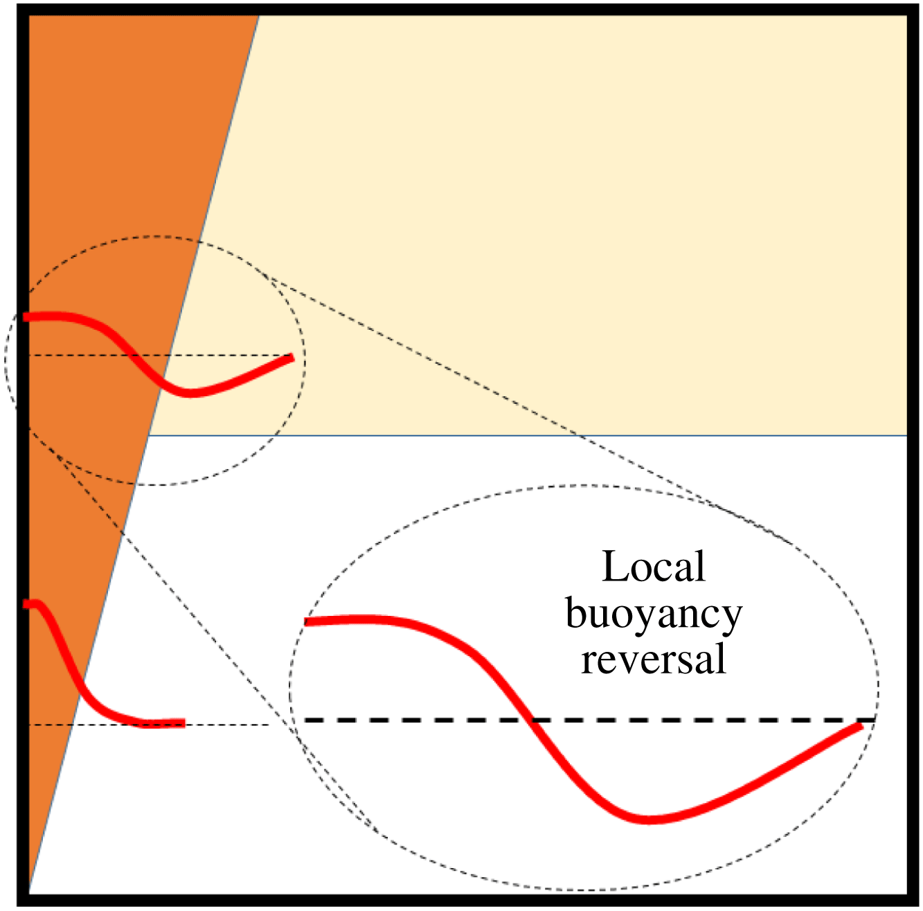
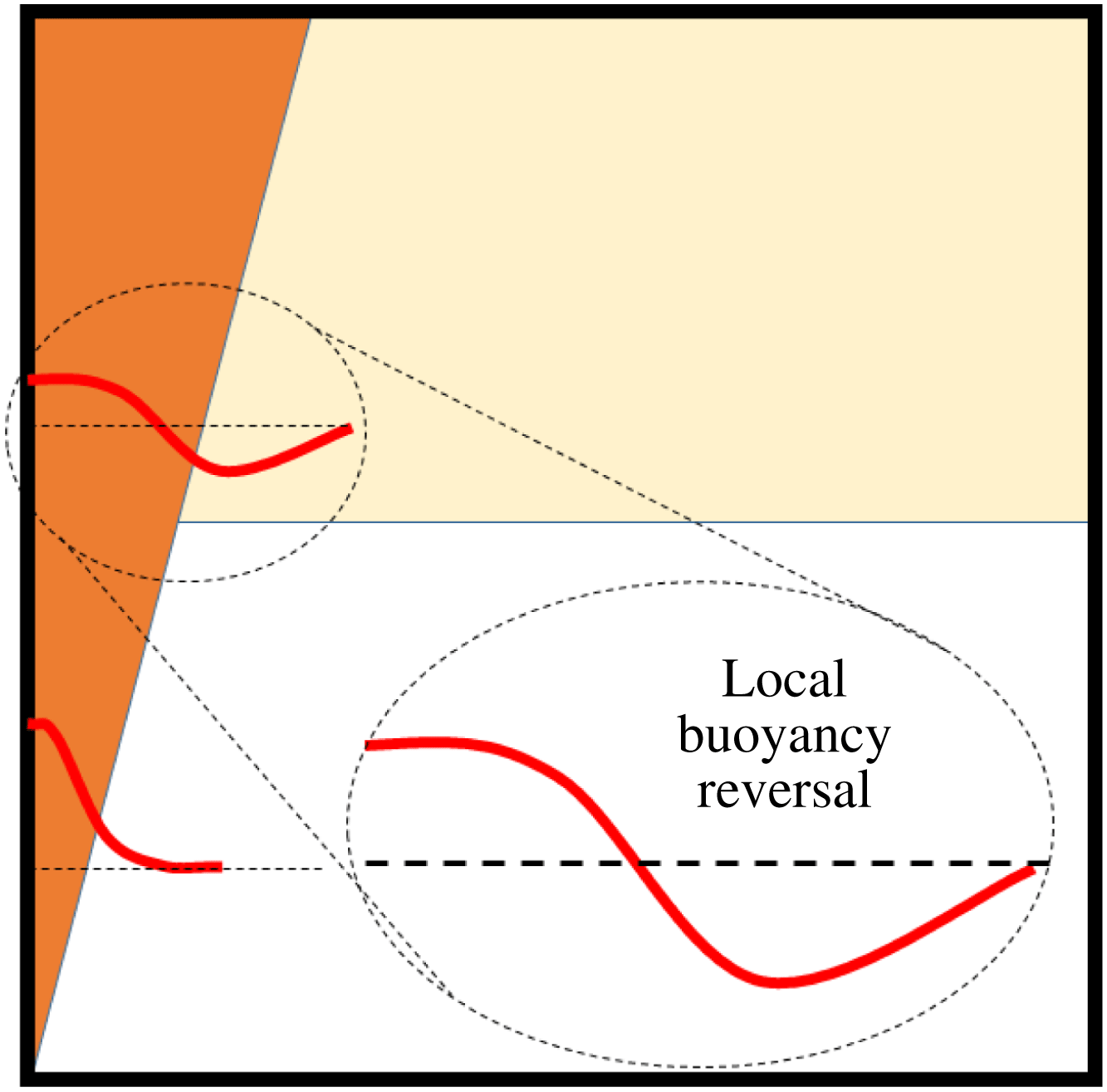
Typical models for detrainment under these circumstances examine the transverse distribution of buoyancy away from the plume or gravity current centreline. When the flow reaches a sharp density interface, some of the outer portion of the plume or gravity current flow is less buoyant than the fluid on the other side of the density step (so-called local buoyancy reversal) and is unable to penetrate the upper layer – see figure 1 in this paper or figure 4(a) in GW. For example, Cortes et al. (Reference Cortes, Rueda and Wells2014) predicted the portion of the gravity current that was unable to penetrate a density step by assuming that all of the flow that underwent local buoyancy reversal peeled off (detrained). This model agreed well with their experiments. However, the steady-state emptying filling-box model of Linden et al. (Reference Linden, Lane-Serff and Smeed1990) results in a vertical plume impinging on a density interface that has a buoyancy step equal to the average buoyancy of the plume at that height. In this case there is, therefore, substantial buoyancy reversal at this location but no detrainment is observed. It should also be noted that the flow of a gravity current down a slope through a horizontal density step is quantitatively different from that of a vertical plume passing through a similar density change. First, for a gravity current flowing down a slope, at the height of the density step the flow has a component of momentum that is parallel to the density interface whereas the vertical plume does not. Second, the buoyancy force driving the gravity current is only the component acting down the slope whereas the plume is vertical. Both of these differences will make the gravity current more susceptible to peeling due to local buoyancy reversal.
Schematic diagram showing a wall plume (on the left wall) crossing a density interface. Local buoyancy profiles are shown below and above the density step. The density step results in the sign of the plume buoyancy reversing locally at the outer edges of the plume.
It is the goal of this paper to examine the impact of the source mass flux and wall shear stress on the dynamics of a vertically distributed plume and its implications for the modelling of such plumes when they are located in a finite enclosure. The paper focuses on the salt plume experiments of CH, GW and BCL. The observations and results of MK’s ice-wall experiments and how they differ from salt plume experiments are also discussed. The remainder of the paper is structured as follows. In § 2 we present analysis of vertically distributed wall plumes. We review the plume equations for a vertically distributed planar source of mass and buoyancy, and examine the impact of the source mass flux on the plume development and its impact on the first front movement in a filling box. We then analyse the impact of these results on previously published experimental results that used the salt bath technique (CH; BCL). Finally we examine the role of the wall shear stress on the plume development. Vertically distributed line sources of buoyancy are discussed in § 3 covering the same topics as for wall plumes. The possible implications for plume entrainment and detrainment are discussed in § 4 and conclusions are drawn in § 5.
For clarity, the remainder of the paper will use the following terminology for the different plume geometries. For consistency, the geometry will describe the distribution of the source of buoyancy. Therefore, a wall plume is a planar plume with the buoyancy source distributed over a vertical plane (wall). A horizontal line plume is the equivalent planar plume with the source buoyancy concentrated along a horizontal line at the base of the plume. A vertical line plume is a round plume with the buoyancy source distributed vertically along a line; and a point-source plume is the analogous round plume with the buoyancy source concentrated at a point at the base of the plume.
2 Source and boundary condition effects on wall plumes
Herein we examine the impact of source volume flux and wall shear stress on the flow of a wall plume. We initially examine the role of source conditions on the flow of an unconfined wall plume followed by an analysis of confined wall plumes. The impact of non-ideal source conditions on previously published salt bath experiments on confined wall plumes is then discussed, followed by an analysis of the role of wall shear stress on the flow development.
2.1 Unconfined wall plumes
We consider a vertical wall of width
 $W$
with a uniformly distributed flux of buoyant fluid, that is a flux of both mass and buoyancy, in an unstratified quiescent ambient. The flux of buoyant fluid produces a vertical wall plume that rises and entrains ambient fluid. The buoyant fluid is added at a rate
 $q$
(
 $\text{m}^{3}~\text{s}^{-1}~\text{m}^{-2}$
) with a density
 $\unicode[STIX]{x1D70C}_{W}$
. We assume that the density ratio
 $\unicode[STIX]{x1D70C}_{a}/\unicode[STIX]{x1D70C}_{W}$
is small such that the Boussinesq assumption is valid. Therefore, without loss of generality, we assume that the fluid source density is less than the ambient density
 $\unicode[STIX]{x1D70C}_{a}$
. All density differences are parametrized in terms of a reduced gravity or buoyancy defined in (1.2). The wall buoyancy flux per unit area is given by
 $f=qg_{W}^{\prime }$
(
 $\text{m}^{4}~\text{s}^{-3}~\text{m}^{-2}$
). The subscript ‘
 $W$
’ denotes a wall-source value.
At any given height the plume can be characterized in terms of vertical fluxes per unit width of volume
 $Q$
, momentum per unit mass
 $M$
and buoyancy
 $F$
. Assuming top-hat profiles for velocity and buoyancy, the fluxes per unit width are given by
 $$\begin{eqnarray}Q=ub,\quad M=u^{2}b\quad \text{and}\quad F=g^{\prime }Q,\end{eqnarray}$$
where
 $u$
is the mean vertical velocity and
 $b$
is the plume width normal to the wall. (Top-hat profiles are used for mathematical convenience. The profiles of velocity and buoyancy are assumed to be uniform out to the plume edge and zero at greater distances from the plume axis – see for example Kaye (Reference Kaye1998, Reference Kaye2008).)
2.1.1 Equations of motion
At some arbitrary height
 $z$
we consider an infinitesimal control volume of width
 $b$
and height
 $\text{d}z$
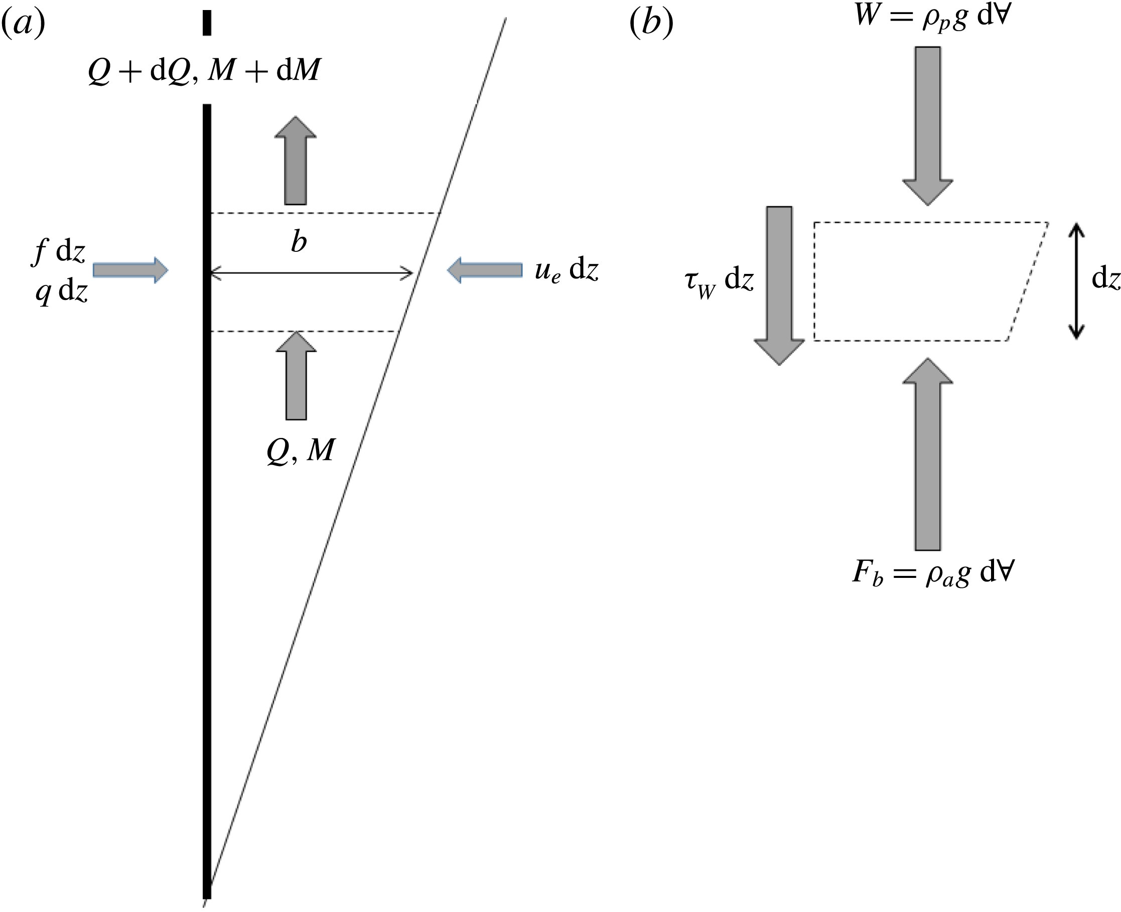
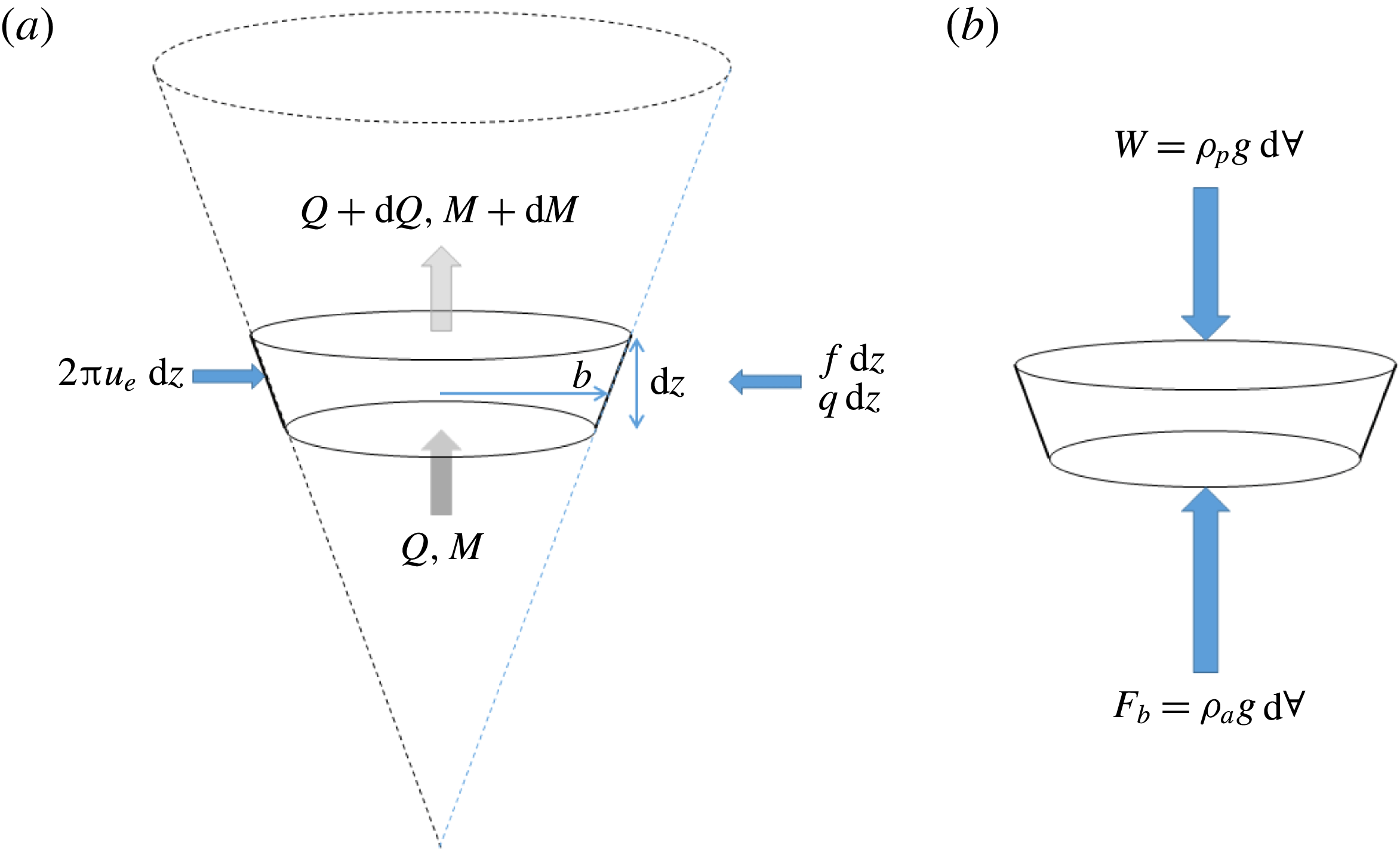
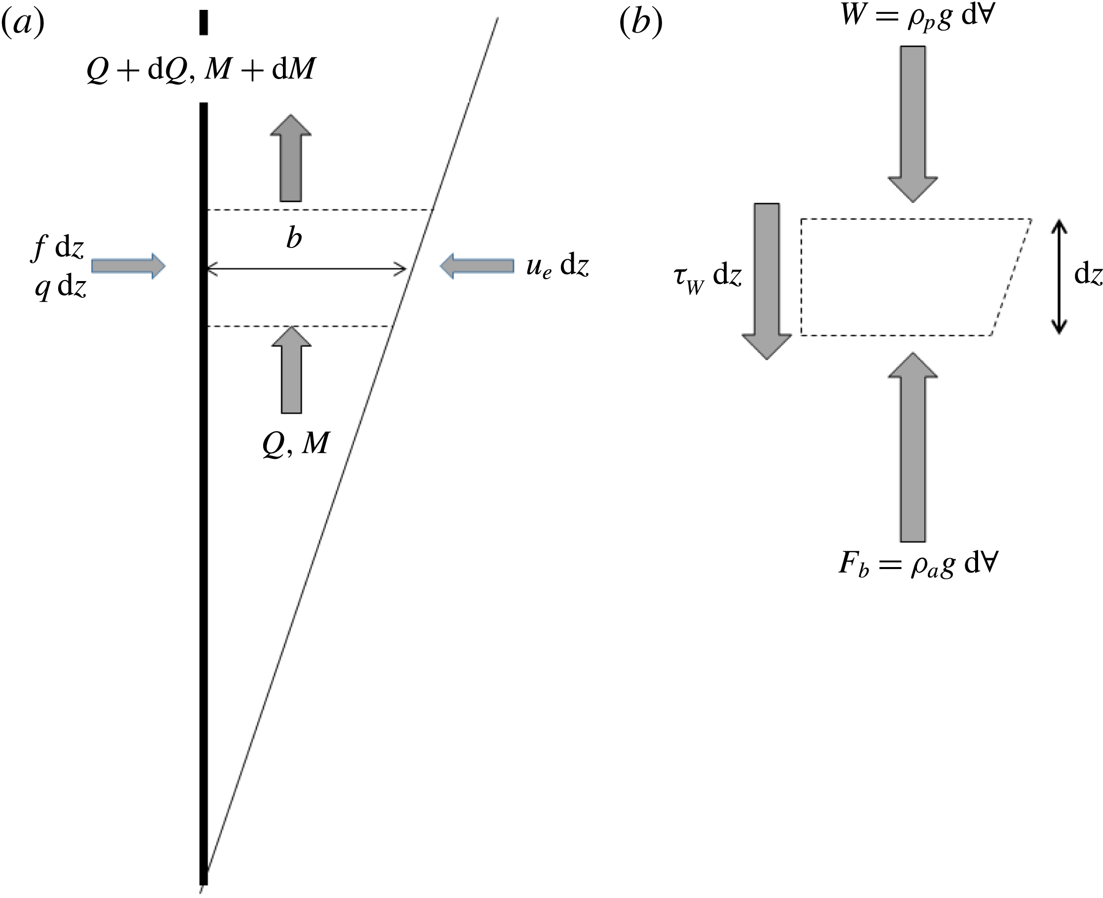
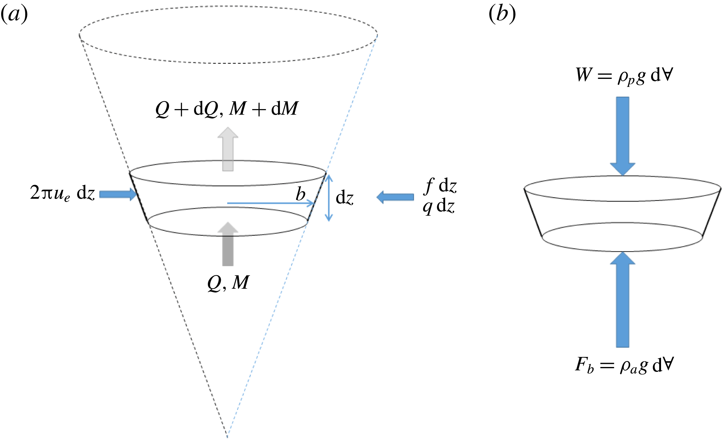
(see figure 2
a). The control volume is fixed in space in a steady flow such that conservation of volume implies that the change in plume volume flux over the control volume is due to the wall-source volume flux and entrainment of ambient fluid, which is taken to be
 $\unicode[STIX]{x1D6FC}u$
, where
 $\unicode[STIX]{x1D6FC}$
is the standard entrainment coefficient (Morton et al.
Reference Morton, Taylor and Turner1956). The change in momentum is due to the net force on the control volume, which, assuming that the plume is long and thin such that the pressure everywhere is hydrostatic, is the difference between the buoyancy force
 $F_{b}$
minus the weight
 $W$
and the wall shear stress
 $\unicode[STIX]{x1D70F}_{W}$
(see figure 2
b). The only change in buoyancy flux is due to the wall-source buoyancy flux.
(a) Schematic diagram of a vertically distributed wall plume showing a control volume of height
 $\text{d}z$
with the inflow of source volume (
 $q$
) and buoyancy (
 $f$
) from the wall and entrainment inflow from the ambient, where
 $u_{e}$
is the entrainment velocity. (b) Forces acting on the control volume (of volume per unit width
 $\text{d}\forall =b\,\text{d}z$
) assuming the pressure is everywhere hydrostatic.
Assuming uniformity in the transverse horizontal direction, the plume equations for the fluxes of volume, momentum and buoyancy flux per unit width are, therefore,
 $$\begin{eqnarray}\frac{\text{d}Q}{\text{d}z}=\unicode[STIX]{x1D6FC}u+q=\unicode[STIX]{x1D6FC}\frac{M}{Q}+q,\quad \frac{\text{d}M}{\text{d}z}=g^{\prime }b-\frac{\unicode[STIX]{x1D70F}_{W}}{\unicode[STIX]{x1D70C}_{a}}=\frac{QF}{M}-C_{f}\frac{M^{2}}{Q^{2}}\quad \text{and}\quad \frac{\text{d}F}{\text{d}z}=f,\end{eqnarray}$$
respectively, where
 $C_{f}$
is the local skin friction coefficient. Note that, while there is a source term included for the volume flux (2.2a
), there is no equivalent forcing term in the momentum equation, as it is assumed that any source momentum is only in the horizontal direction and has no influence on the vertical momentum flux. For the remainder of this subsection we ignore the wall shear stress term, which is considered in § 2.4.
2.1.2 Source conditions and length scales
At the base of the plume (
 $z=0$
) the plume fluxes are
 $Q_{o}=M_{o}=F_{o}=0$
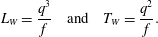
. Therefore, there are no source length scales associated with the base of the plume. However, there are length and time scales associated with the finite sources of volume (
 $q$
) and buoyancy (
 $f$
) along the wall. These are given by
 $$\begin{eqnarray}L_{W}=\frac{q^{3}}{f}\quad \text{and}\quad T_{W}=\frac{q^{2}}{f}.\end{eqnarray}$$
This allows for the definition of a set of non-dimensional fluxes of volume, momentum and buoyancy given by
 $$\begin{eqnarray}\unicode[STIX]{x1D703}=Q\frac{T_{W}}{L_{W}^{2}}=\frac{Q\,f}{q^{4}},\quad \unicode[STIX]{x1D707}=M\frac{T_{W}^{2}}{L_{W}^{3}}=\frac{Mf}{q^{5}}\quad \text{and}\quad \unicode[STIX]{x1D719}=F\frac{T_{W}^{3}}{L_{W}^{3}}=\frac{F}{q^{3}},\end{eqnarray}$$
respectively. The non-dimensional buoyancy, plume thickness, mean velocity and vertical coordinate are given by
 $$\begin{eqnarray}\unicode[STIX]{x1D6FE}=\frac{\unicode[STIX]{x1D719}}{\unicode[STIX]{x1D703}}=\frac{F}{Q}\frac{q}{f},\quad \unicode[STIX]{x1D6FD}=\frac{b}{L_{W}}=\frac{\unicode[STIX]{x1D703}^{2}}{\unicode[STIX]{x1D707}}=\frac{Q^{2}}{M}\frac{f}{q^{3}},\quad \unicode[STIX]{x1D710}=\frac{\unicode[STIX]{x1D707}}{\unicode[STIX]{x1D703}}=\frac{M}{Q}\frac{1}{q}\quad \text{and}\quad \unicode[STIX]{x1D701}=\frac{z}{L_{W}}=\frac{z\,f}{q^{3}},\qquad\end{eqnarray}$$
respectively. The non-dimensional plume equations for the fluxes of volume, momentum and buoyancy are given by
 $$\begin{eqnarray}\frac{\text{d}\unicode[STIX]{x1D703}}{\text{d}\unicode[STIX]{x1D701}}=\unicode[STIX]{x1D6FC}\frac{\unicode[STIX]{x1D707}}{\unicode[STIX]{x1D703}}+1,\quad \frac{\text{d}\unicode[STIX]{x1D707}}{\text{d}\unicode[STIX]{x1D701}}=\frac{\unicode[STIX]{x1D703}\unicode[STIX]{x1D719}}{\unicode[STIX]{x1D707}}\quad \text{and}\quad \frac{\text{d}\unicode[STIX]{x1D719}}{\text{d}\unicode[STIX]{x1D701}}=1,\end{eqnarray}$$
respectively.
The ideal plume fluxes, calculated assuming that the wall-source volume flux is negligible (that is, ignoring the second term on the right-hand side of (2.6a )), are given by
 $$\begin{eqnarray}\unicode[STIX]{x1D703}=\frac{5}{3}\left(\frac{27\unicode[STIX]{x1D6FC}}{100}\right)^{2/3}\unicode[STIX]{x1D701}^{4/3},\quad \unicode[STIX]{x1D707}=\left(\frac{27\unicode[STIX]{x1D6FC}}{100}\right)^{1/3}\unicode[STIX]{x1D701}^{5/3}\quad \text{and}\quad \unicode[STIX]{x1D719}=\unicode[STIX]{x1D701}.\end{eqnarray}$$
The power-law scaling of these fluxes with height differs from the scaling for a horizontal line plume in which the buoyancy flux is constant with height and all the buoyancy is released at the base of the plume. In this case the power-law exponents for the fluxes of volume, momentum and buoyancy are 1,
 $4/3$
and 0, respectively. This result is the same as presented in CH, though with different notation and non-dimensionalization.
The non-dimensional buoyancy, thickness and velocity are given by
 $$\begin{eqnarray}\unicode[STIX]{x1D6FE}=\frac{3}{5}\left(\frac{100}{27\unicode[STIX]{x1D6FC}}\right)^{2/3}\unicode[STIX]{x1D701}^{-1/3},\quad \unicode[STIX]{x1D6FD}=\frac{b}{L_{W}}=\frac{\unicode[STIX]{x1D703}^{2}}{\unicode[STIX]{x1D707}}=\frac{3\unicode[STIX]{x1D6FC}}{4}\unicode[STIX]{x1D701}\quad \text{and}\quad \unicode[STIX]{x1D710}=\frac{3}{5}\left(\frac{100}{27\unicode[STIX]{x1D6FC}}\right)^{1/3}\unicode[STIX]{x1D701}^{1/3},\end{eqnarray}$$
respectively. As with all far-field plume models, the plume thickness grows linearly with distance from the base of the wall source (see Kaye & Scase Reference Kaye and Scase2011).
2.1.3 Comparison with horizontal line plumes
We examine the difference in the variation in volume flux with height between a wall plume and an ideal horizontal line plume with the same total buoyancy flux. Equation (2.7a ) can be used to calculate the dimensional flow rate per unit width for a vertically distributed wall plume as
 $$\begin{eqnarray}Q_{w}=\frac{\unicode[STIX]{x1D703}q^{4}}{f}=\frac{5}{3}\left(\frac{27\unicode[STIX]{x1D6FC}}{100}\right)^{2/3}f^{1/3}z^{4/3}=C_{w}\,f^{1/3}z^{4/3},\end{eqnarray}$$
where
 $$\begin{eqnarray}C_{w}=\frac{5}{3}\left(\frac{27\unicode[STIX]{x1D6FC}}{100}\right)^{2/3}\approx 0.696\unicode[STIX]{x1D6FC}^{2/3}.\end{eqnarray}$$
Solution of (2.2) with
 $q=f=0$
, a constant source buoyancy flux
 $F$
and
 $Q=M=0$
at
 $z=0$
leads to the equivalent expression for the flow rate per unit width of a horizontal line plume. This is given by
 $$\begin{eqnarray}Q_{L}=C_{L}F^{1/3}z,\end{eqnarray}$$
where
 $$\begin{eqnarray}C_{L}=\frac{2\unicode[STIX]{x1D6FC}}{(4\unicode[STIX]{x1D6FC})^{1/3}}\approx 1.26\unicode[STIX]{x1D6FC}^{2/3}.\end{eqnarray}$$
The subscripts ‘
 $W$
’ and ‘
 $L$
’ denote wall and horizontal line plumes, respectively.
We consider two planar plumes, a wall plume and a horizontal line plume. The wall plume source has a height
 $H$
and, unlike the analysis above, forms a plume on both sides of the wall (so that the wall and horizontal line plume flows are qualitatively similar). The buoyancy flux per unit height on each side of the wall is taken to be
 $f=F/2H$
such that the total buoyancy flux in each plume is the same at the height
 $z=H$
. The volume flux for the vertically distributed plume will be twice that given in (2.9) for the prescribed
 $f$
. Assuming that the entrainment coefficient is the same for both plumes, the ratio of the line plume volume flux to the wall plume volume flux is
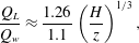 $$\begin{eqnarray}\frac{Q_{L}}{Q_{w}}\approx \frac{1.26}{1.1}\left(\frac{H}{z}\right)^{1/3},\end{eqnarray}$$
where the denominator
 $1.1=0.696\times 2^{2/3}$
. At the top of the plume (
 $z=H$
) the horizontal line plume volume flux is 15 % greater than that of the wall plume. This percentage difference is greater at lower heights. For example, at
 $z=H/2$
the horizontal line plume flow rate is 44 % larger than the wall plume’s. Equation (2.13) shows that, even though the wall plume volume flux scales on
 $z^{4/3}$
, which is greater than for a line plume (
 $z^{1}$
), the flow rate will always be lower in a wall plume due to the lower buoyancy flux at any given height, resulting in less vertical momentum generation and less entrainment.
As an aside, because the buoyancy flux varies with height, it is not possible to define a vertical virtual origin correction to account for the wall-source mass flux, as adding on a virtual origin distance would result in the plume buoyancy flux being incorrect at all heights.
2.1.4 Influence of source inflows
The wall-source volume flux and source fluid buoyancy are compared to the fluxes derived from the ideal plume flow that results from a pure source of buoyancy with no wall volume flux (2.7). As the velocity in the plume scales on height raised to the power of
 $1/3$
, the entrainment rate into the plume (
 $\unicode[STIX]{x1D6FC}u$
) also increases with height such that at large heights the entrainment velocity will be significantly greater than the wall-source volume flux
 $q$
. However, near the base of the plume the entrainment rate will be significantly less than
 $q$
. At any height
 $\unicode[STIX]{x1D701}$
the contribution of the wall source to the total non-dimensional volume flux in the plume will be
 $\unicode[STIX]{x1D703}=\unicode[STIX]{x1D701}$
. Therefore, assuming that (2.7a
) is approximately valid, the entrained volume flux will be of a similar order to the source volume flux when
 $$\begin{eqnarray}\unicode[STIX]{x1D701}=\frac{5}{3}\left(\frac{27\unicode[STIX]{x1D6FC}}{100}\right)^{2/3}\unicode[STIX]{x1D701}^{4/3}\quad \text{or}\quad \unicode[STIX]{x1D701}_{Q}=\frac{80/27}{\unicode[STIX]{x1D6FC}^{2}}\approx \frac{2.96}{\unicode[STIX]{x1D6FC}^{2}}.\end{eqnarray}$$
Therefore, the power-law solution (2.7) will only be valid at significantly greater distances above the source than
 $\unicode[STIX]{x1D701}_{Q}$
.
For a non-ideal source, both the buoyancy flux and the source fluid buoyancy are specified and constant. The non-dimensional buoyancy of the fluid supplied at the wall is
 $\unicode[STIX]{x1D6FE}_{W}=1$
. Therefore, above some height, the wall-source buoyancy for the non-ideal plume will be greater than that predicted by the idealized plume model (2.8a
). A scale estimate of the transition height at which the plume buoyancy (2.8a
) and wall-source buoyancy (
 $\unicode[STIX]{x1D6FE}_{W}=1$
) match will be when
 $$\begin{eqnarray}1=\frac{3}{5}\left(\frac{100}{27\unicode[STIX]{x1D6FC}}\right)^{2/3}\unicode[STIX]{x1D701}^{-1/3}\quad \text{or}\quad \unicode[STIX]{x1D701}_{g^{\prime }}\approx \frac{80/27}{\unicode[STIX]{x1D6FC}^{2}}\approx \frac{2.96}{\unicode[STIX]{x1D6FC}^{2}}.\end{eqnarray}$$
Unsurprisingly this is the same height below which the volume flux is dominated by the source volume flux. Therefore, for a physical source of both buoyancy and volume forming a vertically distributed plume, either the bulk of the plume volume flux is due to the source volume flux rather than from entrainment
 $(\unicode[STIX]{x1D701}<2.96/\unicode[STIX]{x1D6FC}^{2})$
or the wall-source buoyancy will be greater than the mean plume buoyancy
 $(\unicode[STIX]{x1D701}>2.96/\unicode[STIX]{x1D6FC}^{2})$
, potentially resulting in significant non-self-similarity in the horizontal buoyancy profiles of the plume. Both of these situations will influence the fluid mechanics of a confined or semi-confined vertically distributed plume and are discussed in later sections.
Below this transition height, the plume flux solution differs considerably from (2.7). Near the base of the plume, net entrainment is very small and the volume flux in the plume is dominated by the wall-source flux of volume such that the non-dimensional volume flux is given by
 $\unicode[STIX]{x1D703}=\unicode[STIX]{x1D701}$
and
 $\unicode[STIX]{x1D6FE}_{P}\approx \unicode[STIX]{x1D6FE}_{W}$
. The buoyancy flux also increases linearly with height such that
 $\unicode[STIX]{x1D719}=\unicode[STIX]{x1D701}$
. Substituting these values into (2.6) and ignoring the entrainment term in (2.6a
) allows calculation of the plume momentum flux, which is given by
 $$\begin{eqnarray}\unicode[STIX]{x1D707}=\sqrt{\frac{2}{3}}\unicode[STIX]{x1D701}^{3/2}.\end{eqnarray}$$
The plume buoyancy, velocity and thickness are given by
 $$\begin{eqnarray}\unicode[STIX]{x1D6FE}=1,\quad \unicode[STIX]{x1D710}=\sqrt{\frac{2}{3}}\unicode[STIX]{x1D701}^{1/2}\quad \text{and}\quad \unicode[STIX]{x1D6FD}=\sqrt{\frac{3}{2}}\unicode[STIX]{x1D701}^{1/2},\end{eqnarray}$$
respectively.
The non-dimensional equations (2.6) were solved numerically over the range
 $10^{-4}<\unicode[STIX]{x1D701}<10^{6}$
with
 $\unicode[STIX]{x1D6FC}=0.1$
using the MATLAB built-in ordinary differential equation (ODE) solver ode15s. Calculations were run for both the full set of equations and the idealized plume equations, that is, equations (2.6) with the source volume flux term neglected in (2.6a
). The initial conditions for the numerical integration of the full set of equations were calculated using the analytic solution for small
 $\unicode[STIX]{x1D701}$
given in (2.16) and (2.17). The initial conditions for the idealized numerical integration were calculated using (2.7). Results of the numerical integrations for the non-dimensional fluxes of momentum (
 $\unicode[STIX]{x1D707}$
) and volume (
 $\unicode[STIX]{x1D703}$
) and the mean plume buoyancy (
 $\unicode[STIX]{x1D6FE}$
) and velocity (
 $\unicode[STIX]{x1D710}$
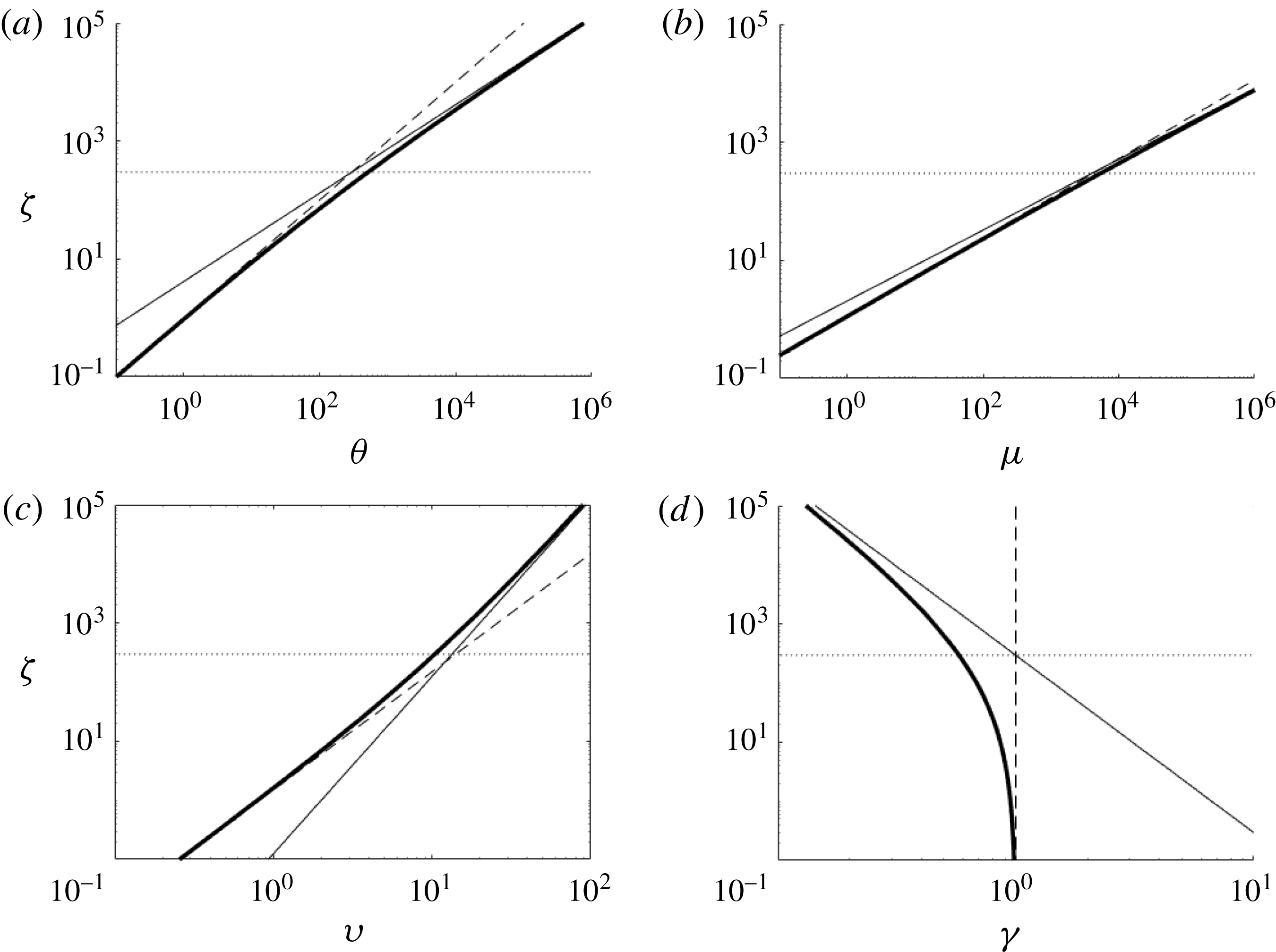
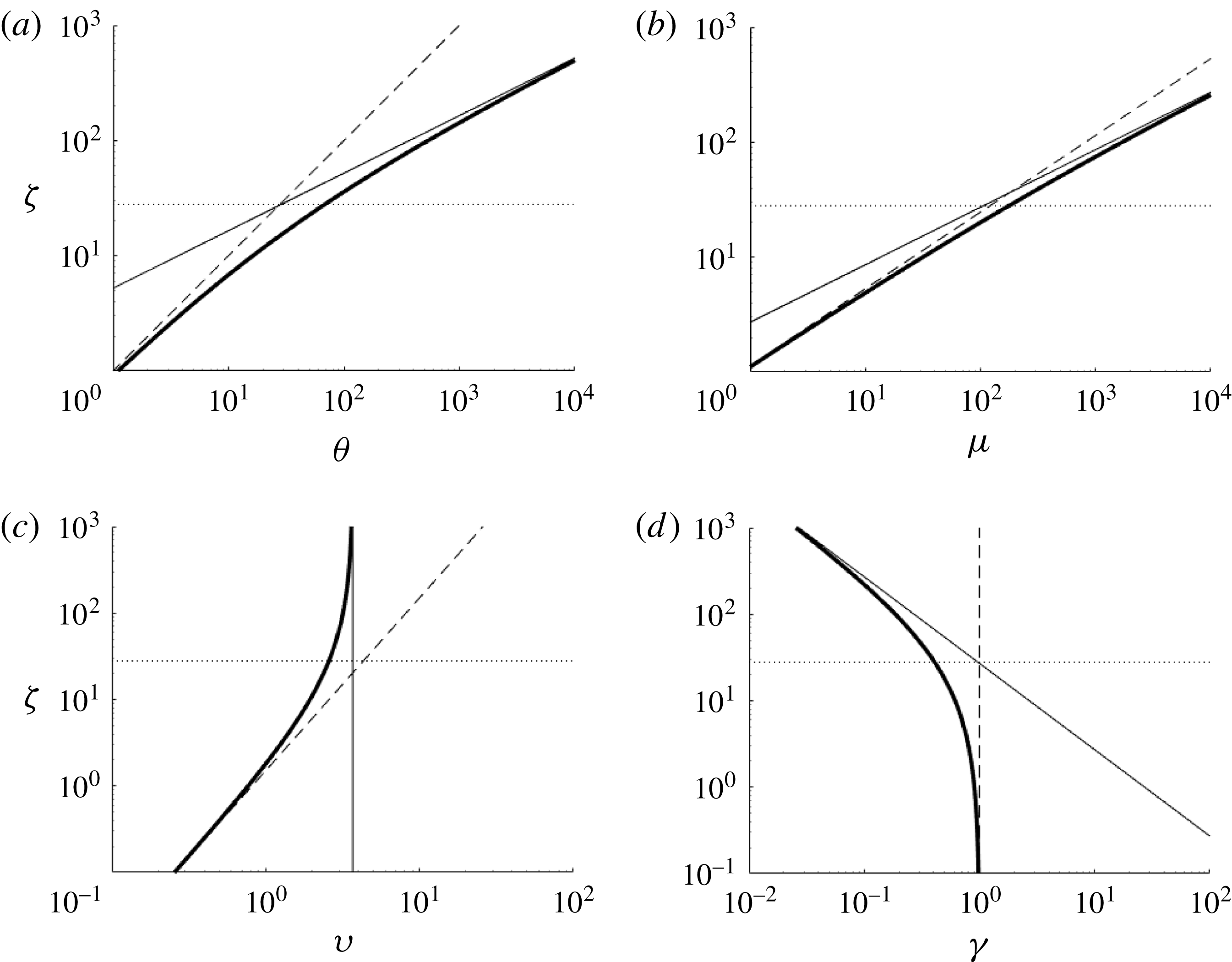
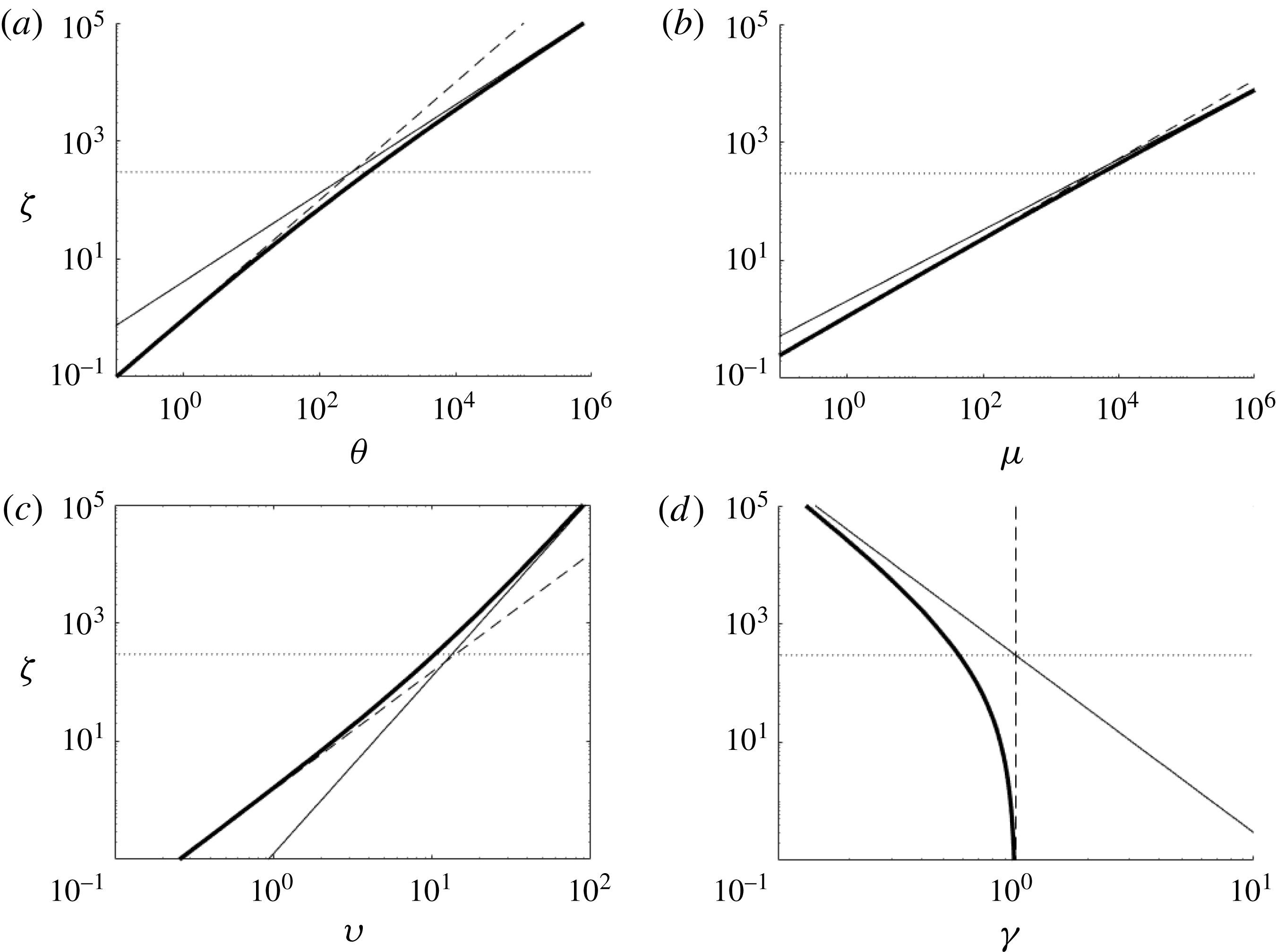
) are shown in figure 3 along with the analytical solution for the flow near the plume base (2.16) and (2.17). For small
 $\unicode[STIX]{x1D701}$
the non-ideal source solution (thick lines) matches the near-source solution in (2.16) and (2.17) (dashed lines). For larger heights the solution approaches the ideal source solution (2.7) and (2.8) (thick line).
Plots of plume parameters for an ideal (thin line) plume source, a non-ideal (thick line) plume source, and the solution for non-ideal flow near the base of the plume (dashed line) determined from (2.16) and (2.17). The horizontal dotted line is at a height
 $\unicode[STIX]{x1D701}_{Q}$
defined in (2.14). From top left they are (a) momentum flux, (b) volume flux, (c) mean velocity and (d) mean buoyancy, respectively. Solutions were calculated for
 $\unicode[STIX]{x1D6FC}=0.1$
and the initial conditions described directly below equation (2.17).
Eventually the solutions converge, as the rate at which ambient fluid is entrained into the plume increases with height and eventually dwarfs the rate at which it is added by the non-ideal source. For the entrainment coefficient considered in figure 3 (
 $\unicode[STIX]{x1D6FC}=0.1$
)
 $\unicode[STIX]{x1D701}_{g^{\prime }}=\unicode[STIX]{x1D701}_{Q}=296$
. (There are a broad range of values for the entrainment coefficient for planar plumes. The choice of
 $\unicode[STIX]{x1D6FC}=0.1$
is illustrative.) The numerical results shown in figure 3 indicate that at
 $\unicode[STIX]{x1D701}=296$
the non-ideal source plume volume and momentum fluxes are 73 % and 35 % larger than the respective fluxes in the ideal plume. Therefore, the length scales in (2.14) and (2.15) do provide a scale for which the two solutions are of equal order, but underestimate the height at which the plume behaves like an ideal wall plume with no wall-source volume flux (a so-called pure plume). To illustrate the height over which the transition to a pure plume occurs, we plot the ratio of the ideal source solution (subscript ‘
 $i$
’) to the finite volume flux solution (subscript ‘
 $f$
’) for the volume flux, momentum flux, plume buoyancy, and plume velocity denoted respectively as
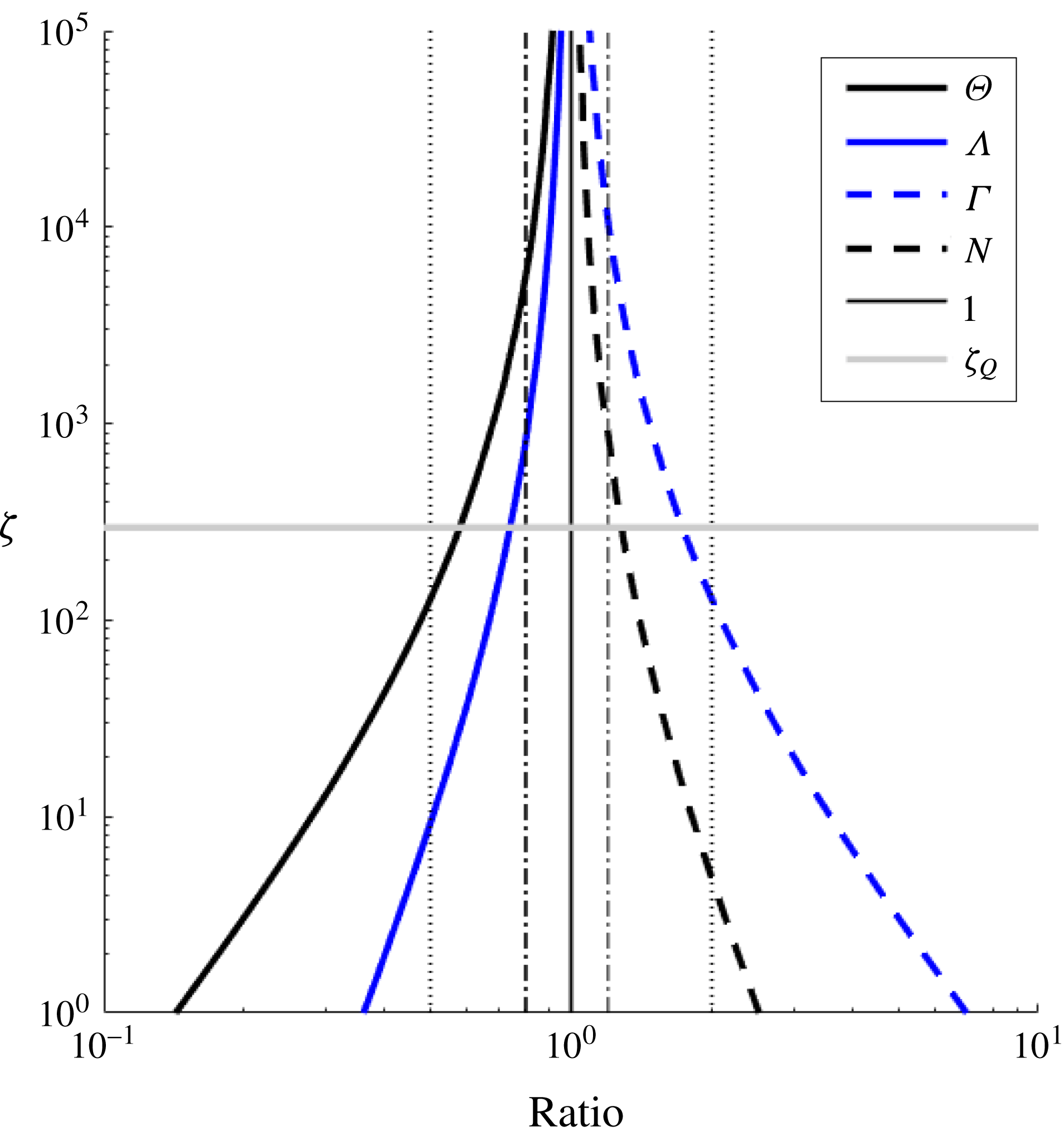
 $$\begin{eqnarray}\unicode[STIX]{x1D6E9}=\frac{\unicode[STIX]{x1D703}_{i}}{\unicode[STIX]{x1D703}_{f}},\quad \unicode[STIX]{x1D6EC}=\frac{\unicode[STIX]{x1D707}_{i}}{\unicode[STIX]{x1D707}_{f}},\quad \unicode[STIX]{x1D6E4}=\frac{\unicode[STIX]{x1D6FE}_{i}}{\unicode[STIX]{x1D6FE}_{f}}\quad \text{and}\quad N=\frac{\unicode[STIX]{x1D710}_{i}}{\unicode[STIX]{x1D710}_{f}}.\end{eqnarray}$$
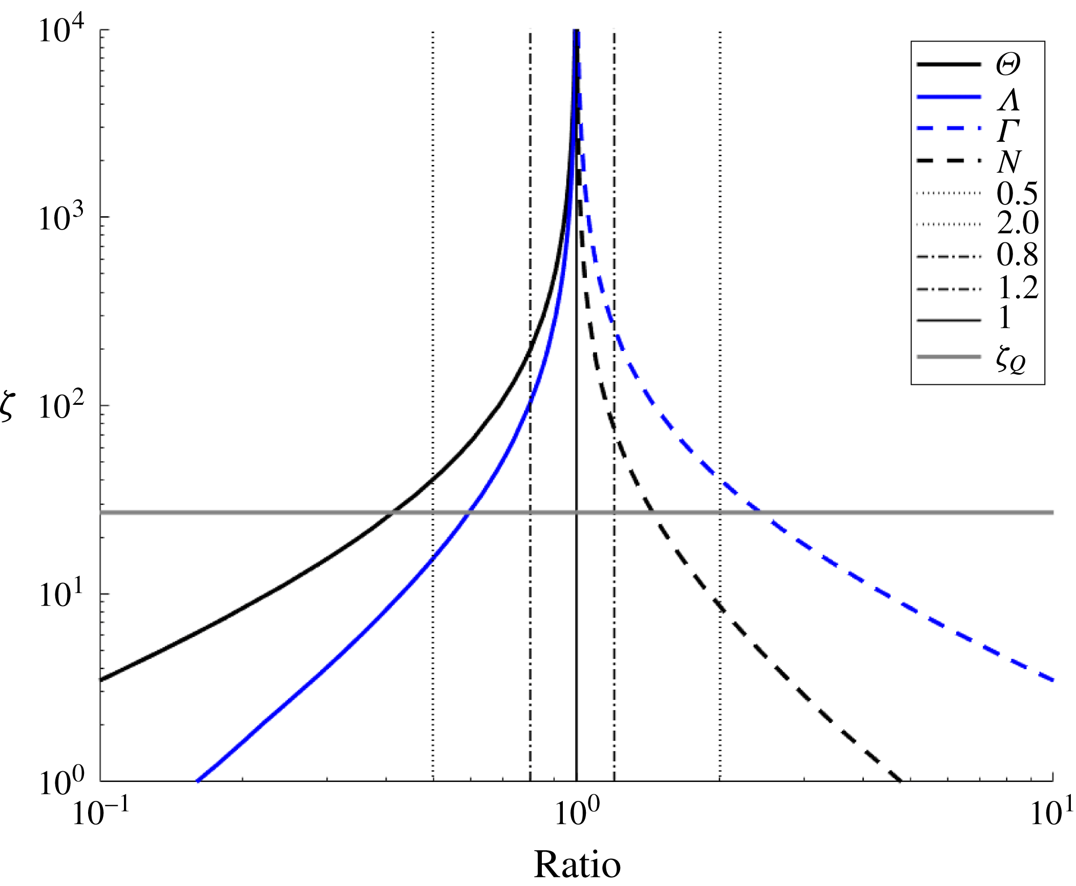
All these ratios will approach 1 as the solutions converge and the source volume flux no longer has any significant influence on the bulk flow properties. This is illustrated in figure 4 in which the ratios are plotted as a function of height. Also shown are vertical lines indicating ratios of 0.5, 0.8, 1.2 and 2 and a horizontal line at a height
 $\unicode[STIX]{x1D701}_{Q}$
.
Plot of the ratio of the ideal source solution (2.7) and (2.8) to the finite volume flux numerical solution to (2.6). Lines are shown for the volume flux, momentum flux, plume buoyancy and plume velocity. The vertical lines indicate ratios of 0.5, 0.8, 1.2 and 2. See (2.18) for definitions of the symbols used in the legend. The data used are from the same numerical integrations used for figure 3 with the same initial conditions.
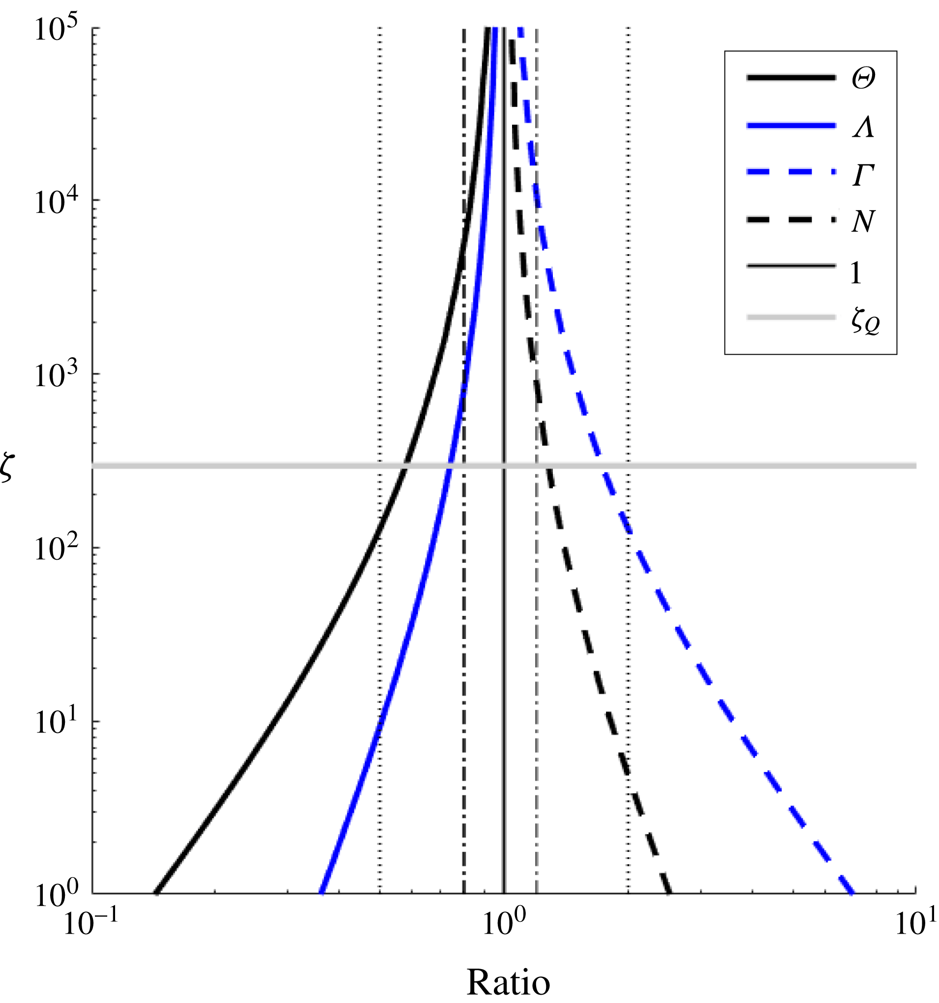
The momentum flux and plume velocity approach the pure plume solution more rapidly. For example, the non-ideal source momentum and velocity are within 20 % of the ideal solution for
 $\unicode[STIX]{x1D701}\approx 800$
whereas the buoyancy and volume fluxes do not achieve this until
 $\unicode[STIX]{x1D701}\approx 6\times 10^{3}$
or approximately
 $20\unicode[STIX]{x1D701}_{Q}$
. Therefore, even if the source length scale
 $L_{W}$
is small compared to other vertical length scales in a given experiment, there could still be significant divergence between the measured and modelled plume volume flux at heights up to
 $6\times 10^{3}\,L_{W}$
. This is particularly important for experiments with confined vertically distributed wall plumes, such as filling-box experiments, as the rate of change of the first front position is dependent on the local volume flux in the plume, which will diverge from ideal analysis as the first front approaches the base of the plume.
2.2 Confined vertically distributed wall plumes
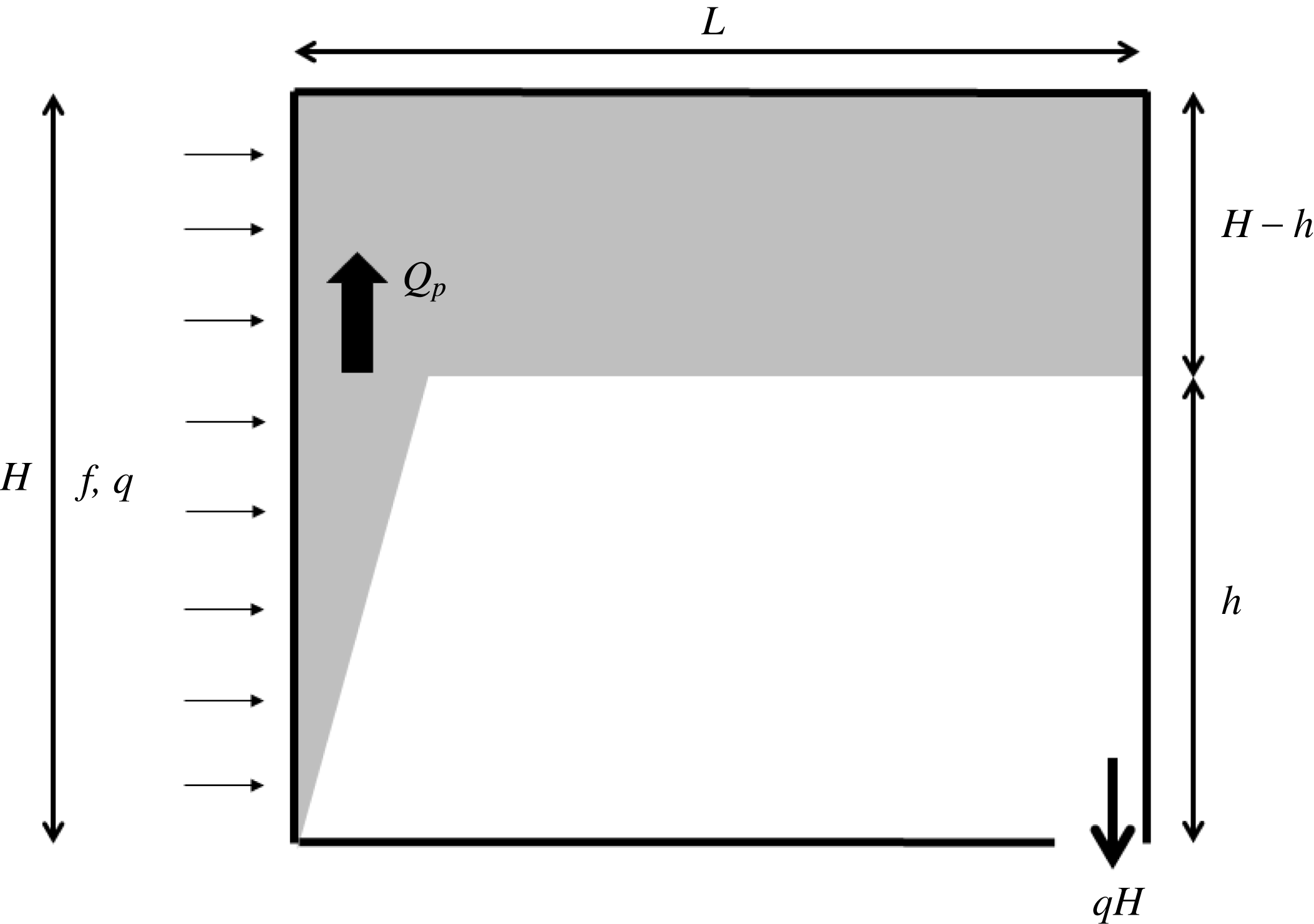
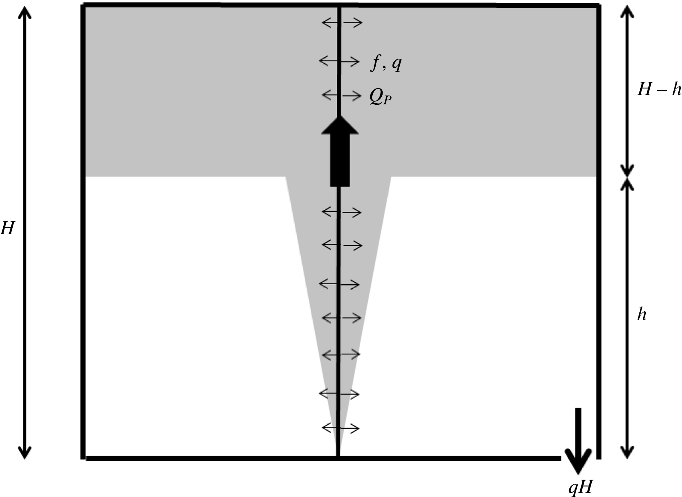
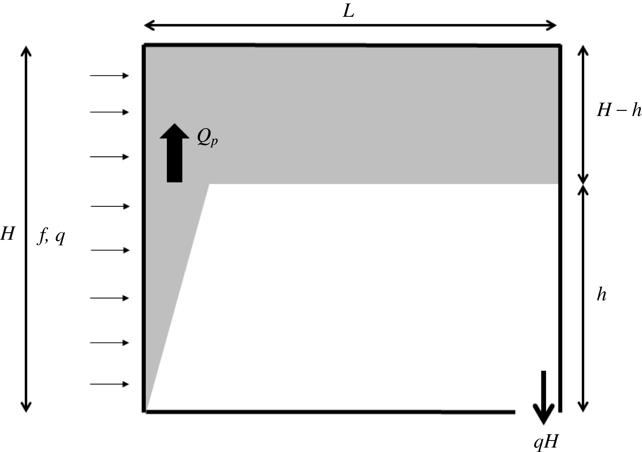
A vertically distributed wall plume placed in a confined region (such as a box) will rise to the top of the box and spread out. The plume fluid that spreads out forms a buoyant upper layer that thickens over time as more plume fluid is added to it. The position of the first front, the interface between the ambient fluid and the upper buoyant fluid layer, moves down over time, eventually approaching the base of the plume. This model for a filling box was first described by Baines & Turner (Reference Baines and Turner1969) for a constant buoyancy flux round plume and was developed as a conceptual model of a mechanism for stratification within a lake or sea. The model has since been extended to the problem of a semi-confined plume where the box is connected via vents to a larger ambient fluid volume. In this case there is an ambient flow through the box that results in a steady buoyant layer depth and stratification, a so-called emptying filling box (see Baines Reference Baines1983; Linden et al. Reference Linden, Lane-Serff and Smeed1990). A schematic of a vertically distributed wall plume in a filling box is shown in figure 5.
Schematic diagram of a confined vertically distributed wall plume showing the wall plume flow and upper buoyant layer that thickens over time as plume fluid is added. The outlet at the base drains a volume flux equivalent to the wall-source volume flux.
Recently, confined and semi-confined vertically distributed wall plumes have been examined theoretically and experimentally (CH; BCL). For a vertically distributed plume, the problem is slightly more complex because there are two sources of volume and buoyancy into the buoyant upper layer, namely the plume inflow at the interface and the wall-source fluxes above the interface height. This leads to more complicated buoyancy stratifications in ventilated boxes (see Linden et al. Reference Linden, Lane-Serff and Smeed1990). It has also led to observations of fluid detraining from the plume at different heights within the upper layer and not simply at the plume outflow along the top of the box. Such detrainment has not been observed in filling-box flows with point or horizontal line sources of buoyancy in which the buoyancy flux is constant with height. In this section we briefly review the theory for the first front movement for a vertically distributed wall plume in a filling box (see Baines & Turner (Reference Baines and Turner1969) on filling-box theory) and then examine the impact of a non-ideal source of buoyancy and volume on the front movement.
We consider a box of height
 $H$
, with a wall source of buoyancy of unit width and box length
 $L$
normal to the wall source. The volume of fluid per unit width in the upper buoyant layer is
 $L(H-h)$
, where
 $h$
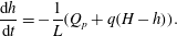
is the height of the interface above the base of the plume (see figure 5). The upper layer volume increases over time due to the inflow of plume fluid from below
 $Q_{p}$
and the inflow of fluid from the non-ideal source
 $q(H-h)$
. Therefore, conservation of volume for the upper layer leads to
 $$\begin{eqnarray}\frac{\text{d}h}{\text{d}t}=-\frac{1}{L}(Q_{p}+q(H-h)).\end{eqnarray}$$
For an ideal source (
 $q=0$
) this can be written, using (2.9), as
 $$\begin{eqnarray}\frac{\text{d}h}{\text{d}t}=-\frac{C_{w}\,f^{1/3}}{L}h^{4/3}.\end{eqnarray}$$
Taking
 $t=0$
as the moment the plume first strikes the top of the box (
 $t=0$
when
 $h=H$
) leads to the solution for the first front movement
 $$\begin{eqnarray}\frac{1}{h^{1/3}}=\frac{1}{H^{1/3}}+\frac{C_{w}\,f^{1/3}}{3L}t,\end{eqnarray}$$
where
 $C_{W}$
is defined in (2.10). This can be written in non-dimensional form as
 $$\begin{eqnarray}\frac{1}{\unicode[STIX]{x1D709}^{1/3}}-1=C_{w}\unicode[STIX]{x1D70F},\end{eqnarray}$$
where
 $$\begin{eqnarray}\unicode[STIX]{x1D709}=\frac{h}{H},\quad \unicode[STIX]{x1D70F}=\frac{t}{T_{F}}=\frac{H^{1/3}f^{1/3}}{3L}t\end{eqnarray}$$
and
 $T_{F}$
is the filling time scale. The solution in (2.22) will be valid, provided that
 $h$
is large enough such that the front movement is dominated by the plume volume flux at the interface, that is, provided
 $h\gg h_{F}$
, where
 $h_{F}$
is the height at which the two terms on the right-hand side of (2.19) are equal and is given by the solution to
 $$\begin{eqnarray}C_{w}\,f^{1/3}h_{F}^{4/3}=q(H-h_{F}).\end{eqnarray}$$
As an aside, there is an additional difficulty with running filling-box experiments with a vertically distributed plume, namely the delineation of the start time. For a point source or horizontal line source of buoyancy, the start time for the filling-box calculation is taken to be when the top of the plume strikes the top of the box. This is appropriate as the plume is fully developed immediately behind the plume head and the filling-box model assumes that the plume spreads out in an infinitesimally thin layer at the top of the box. However, for a wall or vertical line plume the start time is less clearly defined. When the plume is first turned on, the plume source fluid released near the top of the box will immediately strike the top of the box and begin to drive the first front downwards. However, at this time, the plume is not fully developed, as it is not influenced by the source fluid released at the base of the box. There is, therefore, an ambiguity in the start time definition equal to the time taken for plume fluid released near the base of the box to reach the top of the box.
2.3 Impact of source conditions on previously published experimental studies
We examine the impact of a non-ideal plume source (
 $q>0$
) on wall plume filling-box measurements using two examples of experiments in the literature (CH; BCL). These two papers present experimental results for the flow induced by a wall plume in an enclosure, though the papers used different approaches to create a vertically distributed wall plume. The goal of this section is to examine the impact of non-ideal source conditions on the first front movement and subsequent estimation of the plume entrainment coefficient in the papers.
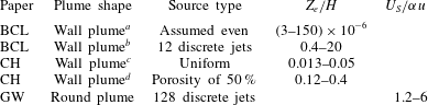
List of input experimental parameters for the experiments of CH and BCL.

a
The tank was filled to a depth of 0.3 m but the traverse only spanned 0.25 m. Further, calculations of
 $q$
based on
 $q=f/g^{\prime }$
and
 $q=Q/A$
imply a vertical distance of 0.25 m.
A wall plume was created by CH using a vertical porous plastic plate to divide their tank into two sections. The smaller section was then supplied with slightly pressurized dense salt solution that was driven through the porous plate, creating a vertical wall supply of dense fluid that was distributed over the entire vertical wall. However, as the flow through the plate was driven by the pressure difference across the plate and that pressure difference varied with height, the flow rate through the wall was not completely uniform. The vertically distributed plume in BCL was created by distributing a series of 12 point sources of buoyant fluid over the surface of one wall of a box. In this case the source flow was not evenly distributed. However, as the flow rate from each of the sources was carefully controlled, the density and flow rate were the same for each source. A summary of the experimental input parameters used in the two papers is given in table 1. In both papers the first front was tracked over time and either the first front position (CH) or the resulting buoyancy profile (BCL) was used to estimate the entrainment coefficient. The length scale
 $L_{W}$
was calculated for each paper using (2.3a
) for each test based on the data in table 1.
In order to assess the influence of experimental wall-source conditions in CH and BCL, numerical calculations were then run to calculate the plume volume flux with height using the full plume flux equations (2.6) and the idealized equations where the source mass flux was ignored. Calculations were run for the entrainment coefficient values presented in the original papers. The data from the numerical integration of the plume equations were then used to calculate the height at which the ideal plume volume flux (2.7a
) was 90 % of the full plume solution (2.6), denoted by
 $L_{90}$
. This length, along with the entrainment coefficient values and the height,
 $h_{F}$
, at which the finite volume flux will significantly influence the first front movement (2.24), are shown in table 2.
List of top-hat entrainment coefficient values and experimental length and time scales for the experiments of CH and BCL.

a
A value of
 $\unicode[STIX]{x1D6FC}=0.02$
was calculated based on a best fit of measured front position to the theoretical front position for an idealized plume source. The value in the table is based on a best fit to a simulation of the plume accounting for the wall volume flux and an estimate of the non-uniformity of the wall volume flux.
b This value is based on a best fit of the measured experimental stratification to the theoretical stratification for a horizontal line plume with constant buoyancy flux. However, the authors took this as appropriate for both the horizontal line plume and vertically distributed wall plume.
The values for the entrainment coefficient are considerably smaller than typical values measured in turbulent line plumes of
 $\unicode[STIX]{x1D6FC}\approx 0.1$
(Paillat & Kaminski Reference Paillat and Kaminski2014). There are a number of potential reasons for this difference. For example, BCL state that their value of
 $\unicode[STIX]{x1D6FC}\approx 0.04$
is likely to be an underestimate as their plume did not spread over the entire width of the source wall (this is not the case for CH, who cite an even lower value). See § 4 for a more detailed discussion of the entrainment coefficient.
CH measured their entrainment coefficient based on the first front movement in a filling-box experiment. They calculated the best fit to the front movement based on a model that was adjusted to include the different non-zero and non-uniform wall-source fluxes that applied in each of the six experiments used to determine
 $\unicode[STIX]{x1D6FC}$
. Their numerical approach, based on the method of Germeles (Reference Germeles1975), implicitly includes the wall-source mass flux above the first front and also accounted for the non-uniform wall mass flux in their experiments.
Simulations were run to replicate a typical experiment from CH and BCL for three different cases. These were (i) a pure plume of buoyancy only, (ii) a plume with a uniform finite wall volume flux but with the source volume flux not considered directly in the first front equation (2.19), and (iii) a uniform finite volume flux plume with the wall volume flux included in (2.19). The two experimental cases considered are test 3 from figure 8 of CH and test I from table 2 of BCL. For each case (2.6) was integrated numerically to calculate the plume volume flux as a function of height. These data were then used to integrate (2.19) to establish the movement of the first front position over time subject to
 $\unicode[STIX]{x1D709}=1$
at
 $\unicode[STIX]{x1D70F}=0$
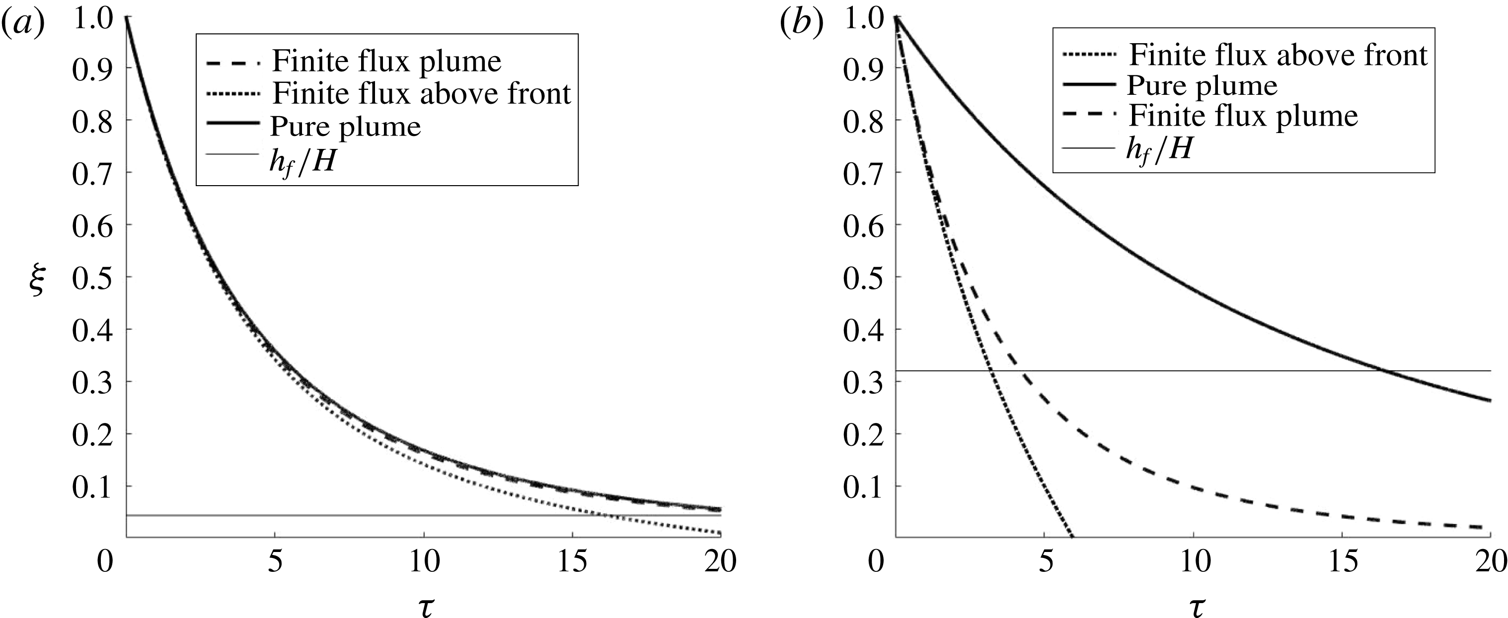
. Results of the non-dimensional front movement for the two experiments simulated for the three cases are shown in figure 6. The entrainment coefficients listed in table 2 were used in the simulations.
The experiments of CH show a much larger disparity between the three cases considered. Table 2 indicates that
 $L_{90}$
is always considerably greater than the box height such that the plume volume flux for the finite source plume is always significantly greater than the pure plume approximation. This is also true when the wall volume flux is included in the first front calculation. The transition height
 $h_{f}$
(defined in (2.24)) at which the wall volume flux contribution to the front movement equals that of the plume is around one-third of the box height.
For the experiments of BCL there is very little difference between the calculated front positions when the wall volume flux in the stratified region below the first front is ignored or included. This is consistent with the data in table 2 which indicate that the height at which the ideal and non-ideal plume fluxes have converged to within 10 % of each other (
 $L_{90}$
) is, at most, 5 % of their box height. However, when the wall volume flux is included in the equation for the first front movement (2.19) there is a slightly larger divergence. This can also be seen in table 2, which shows that the height at which the plume volume flux balances the wall volume flux above the plume (
 $h_{F}$
) is 5–12 % of the box height. Therefore, towards the base of the enclosure the first front will descend more rapidly than predicted if the wall-source volume flux is not included in the calculation.
Plots of the first front position over time for (a) BCL test I (
 $L_{90}/H=8\times 10^{-3}$
) and (b) CH test 3 (
 $L_{90}/H=5.5$
). The solid line is for a pure plume with zero wall-source volume flux, the dashed line includes the wall-source volume flux in the plume calculations only, and the dotted line includes the wall volume flux in both the plume and front movement equations. The thin horizontal line represents the height at which the volume flux in the plume is equal to the wall-source volume flux above the first front as defined in (2.24).
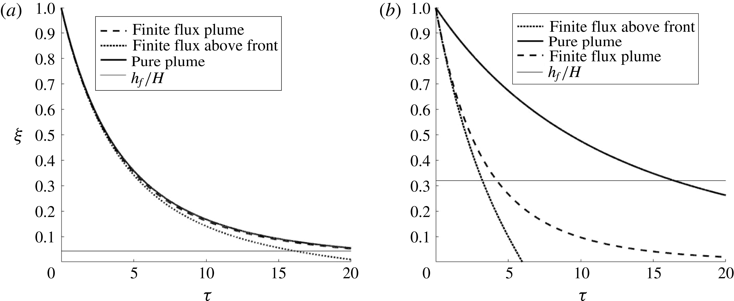
For a wall plume with a finite source volume flux the first front movement will be due to the plume volume flux crossing the first front and the flux of fluid added into the layer above the first front from the wall (2.19). For a finite wall-source volume flux the plume volume flux will be greater than that of a pure plume with no wall-source volume flux and the first front will descend more rapidly. If this is not accounted for in the front calculations and the plume is assumed to be pure, then the additional volume flux in the experimental plume will be erroneously attributed to entrainment and the entrainment coefficient calculated based on first front movement will be overestimated.
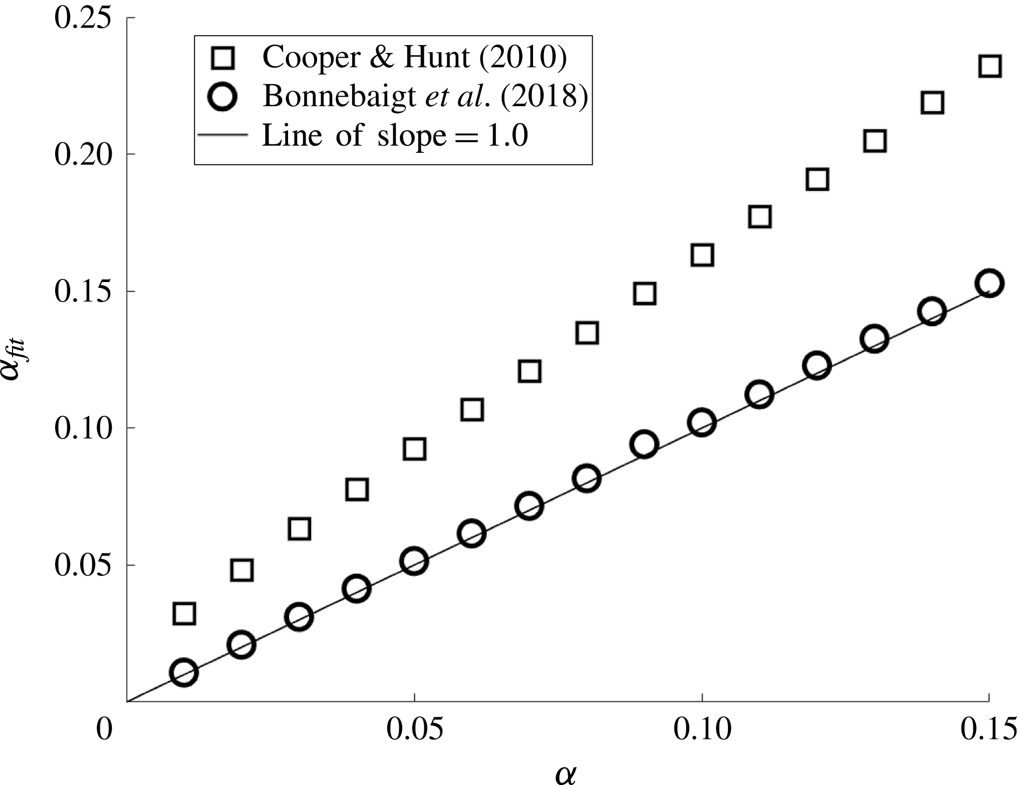
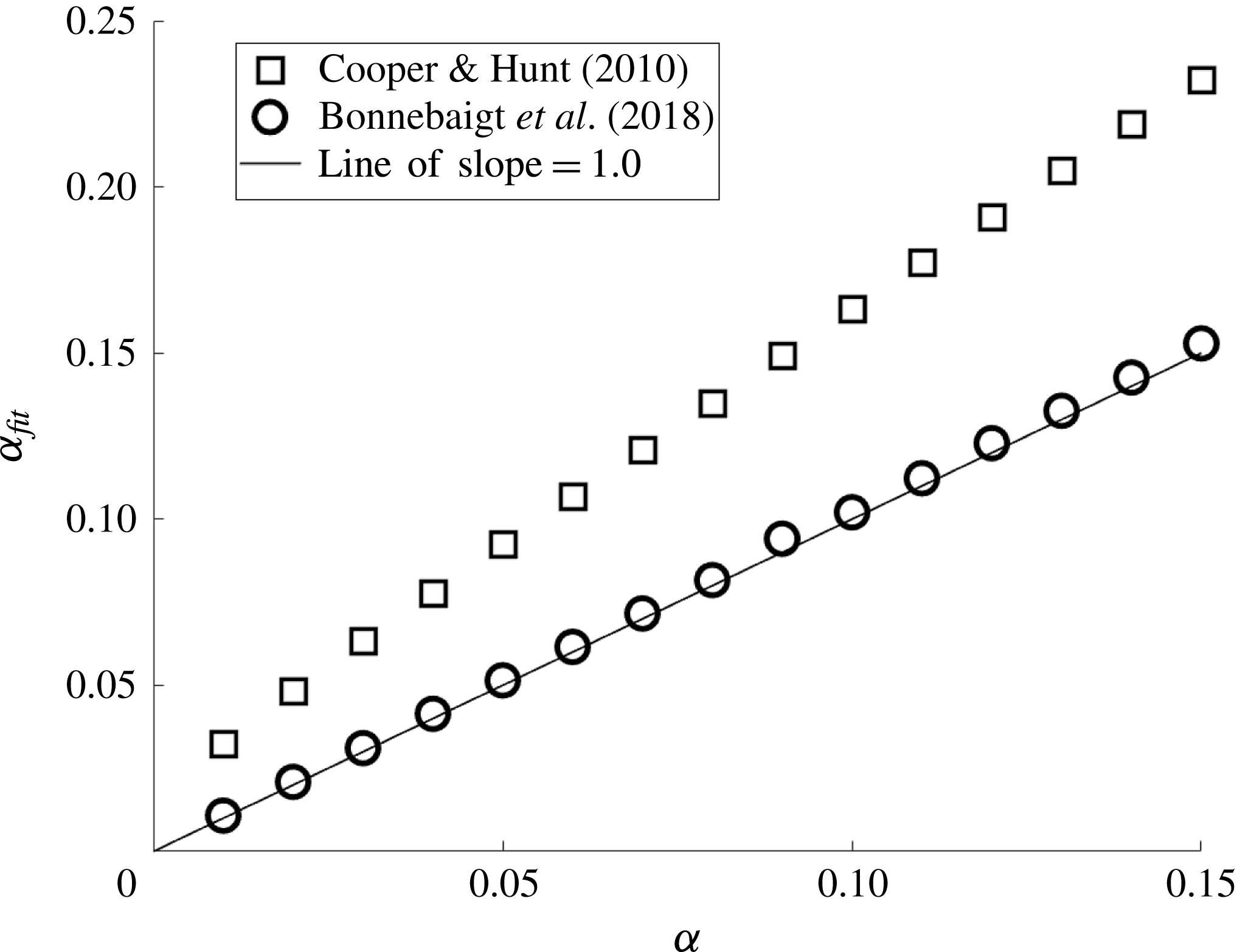
A second series of simulations were run to evaluate this potential impact of the wall volume flux on the experimental estimation of the plume entrainment coefficient. Simulations were run using a range of different entrainment coefficients and the experimental conditions described above. For a given assumed (input) entrainment coefficient, the first front movement was calculated and used to calculate an effective entrainment coefficient based on a fit to the first front data. This
 $\unicode[STIX]{x1D6FC}_{fit}$
is the entrainment coefficient that an experimentalist would calculate if they neglected wall-source volume flux and implicitly attributed that volume flux to entrainment of ambient fluid into the plume.
For each experimental case the entrainment coefficient was varied from 0.01 to 0.15. For each of these entrainment coefficients the plume volume flux was calculated for the case of a uniform finite wall volume flux. These data were then used to calculate the first front position over time. Simulations were run up to
 $\unicode[STIX]{x1D70F}=5$
and the resulting non-dimensional front position was used to calculate the left-hand side of (2.22). This value was then plotted against time, a straight line fitted to establish
 $C_{w}$
, and (2.10) was then used to back-calculate the apparent entrainment coefficient, that is, the entrainment coefficient that, for a pure plume, would give the same front movement. The goal of these calculations is to estimate the error caused by the non-ideal source conditions in the estimation of the plume entrainment coefficient obtained by tracking the first front movement.
The wall volume flux was ignored in the first front calculations (the
 $q(H-h)$
term in (2.19)) as, when it was included, the resulting plot was far from linear and could not be used to reasonably estimate an effective entrainment coefficient. However, qualitatively, the inclusion of this term would increase the value of the calculated entrainment coefficient based on first front movement as the front would descend more rapidly, which would then, erroneously, be attributed to a higher entrainment coefficient. The calculated entrainment coefficient was then plotted against the input entrainment coefficient to evaluate the error in
 $\unicode[STIX]{x1D6FC}$
associated with ignoring the wall volume flux in the plume volume flux. These data are shown in figure 7 using the experimental conditions of CH and BCL. Using this approach shows that the experiments of CH would result in an approximately 60 % overestimation of
 $\unicode[STIX]{x1D6FC}$
. This is consistent with their analysis that showed a 50 % change in
 $\unicode[STIX]{x1D6FC}$
when the wall-source volume flux was included in their plume volume flux calculations. As is expected, based on the length scales presented in table 2, the discrepancy between the input and calculated entrainment coefficients for the BCL simulations was less than 3 %.
Plot of the entrainment coefficient calculated using a best fit through the first front position over time against the entrainment coefficient used in the simulations. Divergence from the line of exact agreement (solid line) implies an error in the estimation of
 $\unicode[STIX]{x1D6FC}$
due to neglecting the finite wall-source volume flux and erroneously attributing this volume flux to plume entrainment.
Clearly the wall-source volume flux plays a significant role in the movement of the first front in a filling box, and the subsequent stratification that develops behind the front. Even for experiments in which the adjustment length scale is very small compared to the box height, as in the tests of BCL, the front movement can still diverge from the pure plume theory.
2.4 Impact of wall shear stress on wall plume flow
We consider the problem of a wall plume in a uniform quiescent ambient in which there is a turbulent wall shear stress retarding the flow. It is assumed that the wall shear stress coefficient (
 $C_{f}$
) is constant such that the stress is given by
 $$\begin{eqnarray}\unicode[STIX]{x1D70F}_{W}=C_{f}\unicode[STIX]{x1D70C}_{a}u^{2},\end{eqnarray}$$
where
 $u$
is the plume velocity. The simplifying assumption of a constant wall shear stress coefficient is consistent with the data presented in Gayen et al. (Reference Gayen, Griffiths and Kerr2016). Equations (2.2a–c
) can then be rewritten as
 $$\begin{eqnarray}\frac{\text{d}Q}{\text{d}z}=\unicode[STIX]{x1D6FC}\frac{M}{Q},\quad \frac{\text{d}M}{\text{d}z}=\frac{QF}{M}-C_{f}\frac{M^{2}}{Q^{2}}\quad \text{and}\quad \frac{\text{d}F}{\text{d}z}=f.\end{eqnarray}$$
For an ideal source with zero fluxes of volume and momentum, the solution to (2.26a–c ) is given by
 $$\begin{eqnarray}Q=\frac{5}{3}\left(\frac{27\unicode[STIX]{x1D6FC}}{100}\right)^{2/3}{\mathcal{F}}^{1/3}z^{4/3},\quad M=\left(\frac{27\unicode[STIX]{x1D6FC}}{100}\right)^{1/3}{\mathcal{F}}^{2/3}z^{5/3}\quad \text{and}\quad F=fz,\end{eqnarray}$$
where
 $$\begin{eqnarray}{\mathcal{F}}=\frac{f}{1+C_{f}{\displaystyle \frac{4}{5\unicode[STIX]{x1D6FC}}}}\end{eqnarray}$$
is the effective buoyancy flux of the plume. That is,
 ${\mathcal{F}}$
is the component of the buoyancy flux that generates vertical momentum and drives the plume, while
 $f-{\mathcal{F}}$
is the component of the buoyancy flux required to overcome the induced wall shear stress. The result in (2.27) is the dimensional equivalent of (2.7) with the effective buoyancy flux replacing the actual buoyancy flux. For the case of zero wall shear stress (
 $C_{f}=0$
) the solution presented in § 2.1 is recovered. This is again consistent with the simulation results of Gayen et al. (Reference Gayen, Griffiths and Kerr2016), who found that the friction and buoyancy forces scaled in the same manner with height.
Flow rate measurements in a plume at different heights that are used to calculate the prefactor in (2.27a
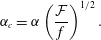
) and then calculate an entrainment coefficient without accounting for wall friction will underestimate the actual entrainment coefficient as predicted by MK. Denoting the entrainment coefficient calculated using the first front movement in a filling-box experiment as
 $\unicode[STIX]{x1D6FC}_{c}$
and equating the ideal (no wall shear stress) flow rate (2.9) with the flow rate calculated when the wall shear stress is modelled (2.27a
) we get
 $$\begin{eqnarray}\frac{5}{3}\left(\frac{27\unicode[STIX]{x1D6FC}}{100}\right)^{2/3}{\mathcal{F}}^{1/3}z^{4/3}=\frac{5}{3}\left(\frac{27\unicode[STIX]{x1D6FC}_{c}}{100}\right)^{2/3}f^{1/3}z^{4/3},\end{eqnarray}$$
which can be solved to give
 $$\begin{eqnarray}\unicode[STIX]{x1D6FC}_{c}=\unicode[STIX]{x1D6FC}\left(\frac{{\mathcal{F}}}{f}\right)^{1/2}.\end{eqnarray}$$
To examine the potential impact of wall shear stress on the estimation of the entrainment coefficient, we consider the ice-melt plume experiments of MK and the salt bath measurements of CH. MK give their entrainment coefficient for a wall plume as
 $\unicode[STIX]{x1D6FC}=0.048$
and provide an estimate of
 ${\mathcal{F}}/f=0.1$
based on their velocity measurements. Using these two values, the calculated entrainment coefficient based on the first front position measurement in which the wall shear stress was ignored would be
 $\unicode[STIX]{x1D6FC}_{c}=0.015$
or approximately half that measured by CH. That is, if MK had calculated their entrainment coefficient based on first front movement rather than direct measurement of the plume velocity, they would get a much lower value. Alternatively, taking the CH value of
 $\unicode[STIX]{x1D6FC}_{c}=0.03$
and the MK value of
 $\unicode[STIX]{x1D6FC}=0.048$
leads to
 ${\mathcal{F}}/f=0.4$
(four times that of MK), which means that only 60 % of the plume buoyancy flux is needed to overcome the wall shear stress for the experiments of CH compared to 90 % for the experiments of MK. This may in part be due to the convective nature of the wall-source condition in which the no-slip boundary condition is replaced with a constant inflow velocity. Clearly though, for wall-bounded flows the wall shear stress plays a role in the flow development and should be accounted for when measuring the plume entrainment coefficient.
3 Unconfined vertical line plumes
The analysis presented for a non-ideal wall plume is now applied to a round vertical line plume with a finite vertical source of buoyancy and volume. The presentation is abbreviated as the analysis is similar to that presented in § 2.
3.1 Unconfined vertical line plumes
We again consider a small control volume of height
 $\text{d}z$
at some arbitrary height
 $z$
above the plume base – see figure 8. In this case the shear stress along the centreline source of buoyancy and mass is neglected (see § 3.4). Invoking the entrainment assumption, the equations for the fluxes of volume, momentum and buoyancy are given by
 $$\begin{eqnarray}\frac{\text{d}Q}{\text{d}z}=2\unicode[STIX]{x1D6FC}\sqrt{M}+q,\quad \frac{\text{d}M}{\text{d}z}=\frac{QF}{M}\quad \text{and}\quad \frac{\text{d}F}{\text{d}z}=f,\end{eqnarray}$$
respectively. In this case
 $Q=ub^{2}$
,
 $M=u^{2}b^{2}$
and
 $F=g^{\prime }Q$
are the fluxes of volume, momentum and buoyancy each divided by
 $\unicode[STIX]{x03C0}$
. The vertical-line-source fluxes of volume and buoyancy are also divided by
 $\unicode[STIX]{x03C0}$
to give
 $q$
and
 $f$
, respectively. For the case when
 $Q_{o}=M_{o}=F_{o}=0$
at
 $z=0$
, there are no length scales associated with the flow at the base of the plume and the only imposed scales are
 $$\begin{eqnarray}L_{S}=\frac{q}{f^{1/3}}\quad \text{and}\quad T_{S}=\frac{q}{f^{2/3}}.\end{eqnarray}$$
The non-dimensional fluxes of volume, momentum and buoyancy can then be written as
 $$\begin{eqnarray}\unicode[STIX]{x1D703}=Q\frac{T_{S}}{L_{S}^{3}}=\frac{Q\,f^{1/3}}{q^{2}},\quad \unicode[STIX]{x1D707}=M\frac{T_{S}^{2}}{L_{S}^{4}}=\frac{M}{q^{2}}\quad \text{and}\quad \unicode[STIX]{x1D719}=F\frac{T_{S}^{3}}{L_{S}^{4}}=\frac{F}{q\,f^{2/3}},\end{eqnarray}$$
respectively. The other non-dimensional parameters (buoyancy, velocity, radius and vertical coordinate) are given by
 $$\begin{eqnarray}\unicode[STIX]{x1D6FE}=\frac{\unicode[STIX]{x1D719}}{\unicode[STIX]{x1D703}}=\frac{F}{Q}\frac{q}{f},\quad \unicode[STIX]{x1D710}=\frac{\unicode[STIX]{x1D707}}{\unicode[STIX]{x1D703}}=\frac{M}{Q}\frac{1}{f^{1/3}},\quad \unicode[STIX]{x1D6FD}=\frac{b}{L_{S}}=\frac{\unicode[STIX]{x1D703}}{\sqrt{\unicode[STIX]{x1D707}}}=\frac{Q}{\sqrt{M}}\frac{f^{1/3}}{q}\quad \text{and}\quad \unicode[STIX]{x1D701}=\frac{z}{L_{S}}=\frac{z\,f^{1/3}}{q},\end{eqnarray}$$
respectively. The non-dimensional flux equations are then written as
 $$\begin{eqnarray}\frac{\text{d}\unicode[STIX]{x1D703}}{\text{d}\unicode[STIX]{x1D701}}=2\unicode[STIX]{x1D6FC}\sqrt{\unicode[STIX]{x1D707}}+1,\quad \frac{\text{d}\unicode[STIX]{x1D707}}{\text{d}\unicode[STIX]{x1D701}}=\frac{\unicode[STIX]{x1D703}\unicode[STIX]{x1D719}}{\unicode[STIX]{x1D707}}\quad \text{and}\quad \frac{\text{d}\unicode[STIX]{x1D719}}{\text{d}\unicode[STIX]{x1D701}}=1.\end{eqnarray}$$
The solutions for the fluxes when
 $\unicode[STIX]{x1D703}_{o}=\unicode[STIX]{x1D707}_{o}=\unicode[STIX]{x1D719}_{o}=0$
at
 $\unicode[STIX]{x1D701}=0$
and the second term on the right-hand side of (3.5a
) is ignored (that is, for a plume with a pure source of buoyancy and no source mass flux) are
 $$\begin{eqnarray}\unicode[STIX]{x1D703}=2\left(\frac{\unicode[STIX]{x1D6FC}}{2}\right)^{4/3}\unicode[STIX]{x1D701}^{2},\quad \unicode[STIX]{x1D707}=\left(\frac{\unicode[STIX]{x1D6FC}}{2}\right)^{2/3}\unicode[STIX]{x1D701}^{2}\quad \text{and}\quad \unicode[STIX]{x1D719}=\unicode[STIX]{x1D701}.\end{eqnarray}$$
Solutions for the buoyancy, radius and plume velocity are given by
 $$\begin{eqnarray}\unicode[STIX]{x1D6FE}=\frac{1}{2}\left(\frac{2}{\unicode[STIX]{x1D6FC}}\right)^{4/3}\unicode[STIX]{x1D701}^{-1},\quad \unicode[STIX]{x1D6FD}=\frac{\unicode[STIX]{x1D703}}{\sqrt{\unicode[STIX]{x1D707}}}=2\unicode[STIX]{x1D6FC}\unicode[STIX]{x1D701}\quad \text{and}\quad \unicode[STIX]{x1D710}=\frac{1}{2}\left(\frac{2}{\unicode[STIX]{x1D6FC}}\right)^{2/3},\end{eqnarray}$$
respectively. This solution is the same as presented by GW, though with a different non-dimensional scheme.
(a) Schematic diagram of a vertical-line-source plume showing a control volume of height
 $\text{d}z$
with the inflow of source volume (
 $q$
) and buoyancy (
 $f$
) from the source (shown externally for convenience) and entrainment inflow from the ambient. (b) Forces acting on the control volume (of volume
 $\text{d}\forall =\unicode[STIX]{x03C0}b^{2}\,\text{d}z$
) assuming the pressure is everywhere hydrostatic.
3.1.1 Comparison with constant buoyancy flux round plume
As with the wall plume, the power-law exponents for the increase in volume and momentum fluxes with height are greater than for a round plume with constant buoyancy flux. For the vertically distributed plume, the volume and momentum fluxes both increase with height squared compared to exponents of
 $5/3$
and
 $4/3$
, respectively, for constant buoyancy flux plumes. The dimensional volume flux is given by
 $$\begin{eqnarray}Q_{VL}=\unicode[STIX]{x03C0}q^{2}f^{-1/3}\unicode[STIX]{x1D703}=\unicode[STIX]{x03C0}^{2/3}\unicode[STIX]{x1D6FC}^{4/3}2^{-1/3}\hat{f}^{1/3}z^{2}=C_{VL}\,\hat{f}^{1/3}z^{2},\end{eqnarray}$$
where the subscript ‘
 $VL$
’ indicates a vertical line plume,
 $\hat{f}=\unicode[STIX]{x03C0}f$
is the actual buoyancy flux per unit height, and
 $$\begin{eqnarray}C_{VL}=\unicode[STIX]{x03C0}^{2/3}\unicode[STIX]{x1D6FC}^{4/3}2^{-1/3}\approx 1.7\unicode[STIX]{x1D6FC}^{4/3}.\end{eqnarray}$$
For a pure constant buoyancy flux round plume the flow rate is given by
 $$\begin{eqnarray}Q_{P}\approx 2.5\unicode[STIX]{x1D6FC}^{4/3}F^{1/3}z^{5/3}\end{eqnarray}$$
(Kaye Reference Kaye2008), where the subscript ‘
 $P$
’ indicates an ideal point-source plume. For a plume with total buoyancy flux
 $F$
and height
 $H$
, the buoyancy flux per unit height for the vertically distributed plume is
 $\hat{f}=F/H$
. The ratio of the point-source plume volume flux to the vertical line plume volume flux and any height
 $z$
is
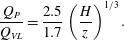 $$\begin{eqnarray}\frac{Q_{P}}{Q_{VL}}=\frac{2.5}{1.7}\left(\frac{H}{z}\right)^{1/3}.\end{eqnarray}$$
As with the horizontal line plume to wall plume comparison, the point-source plume has a significantly greater volume flux at all heights below
 $z=H$
compared with the vertical line plume.
3.1.2 Influence of source inflows
At any height
 $\unicode[STIX]{x1D701}$
the added non-dimensional volume flux will be
 $\unicode[STIX]{x1D703}=\unicode[STIX]{x1D701}$
and the entrained volume flux will be of a similar order to the source volume flux when
 $$\begin{eqnarray}\unicode[STIX]{x1D703}=\unicode[STIX]{x1D701}=2\left(\frac{\unicode[STIX]{x1D6FC}}{2}\right)^{4/3}\unicode[STIX]{x1D701}^{2}\quad \text{or}\quad \unicode[STIX]{x1D701}_{Q}\approx \frac{1.3}{\unicode[STIX]{x1D6FC}^{4/3}}.\end{eqnarray}$$
Therefore, the power-law solution (3.6) will only be valid at significantly greater distances. The non-dimensional buoyancy in the plume is given by (3.7a
), whereas the buoyancy supplied at the source is
 $\unicode[STIX]{x1D6FE}_{S}=1$
. Therefore, above some height, the wall-source buoyancy will be greater than that of the plume. Prior to that the vertical-line-source buoyancy will be less than that of the equivalent pure vertical line plume source of pure buoyancy. The transition height at which the plume buoyancy and wall-source buoyancy match will be when
 $\unicode[STIX]{x1D6FE}=1$
in (3.7a
), or
 $\unicode[STIX]{x1D701}_{g^{\prime }}\approx 1.3/\unicode[STIX]{x1D6FC}^{4/3}$
, which is the same transition height as for the flow rate (3.12).
For low heights in a finite volume flux vertical-line-source plume, the volume flux growth is dominated by the vertical-line-source inflow and is given by
 $\unicode[STIX]{x1D703}=\unicode[STIX]{x1D701}$
. Similarly, the plume buoyancy flux also increases linearly with height (
 $\unicode[STIX]{x1D719}=\unicode[STIX]{x1D701}$
). Substituting these relationships into (3.5b
) gives the momentum flux as
 $$\begin{eqnarray}\unicode[STIX]{x1D707}=\sqrt{\frac{2}{3}}\unicode[STIX]{x1D701}^{3/2},\end{eqnarray}$$
which is identical to the wall plume result in (2.16). The wall plume and the vertical-line-source plume are identical in this region because there is negligible entrainment and only the entrainment term in (3.5) is influenced by the geometry of the plume. As with the wall plume, the vertically distributed round plume with a non-ideal source has a lower power-law exponent for the momentum flux than the ideal source case (
 $3/2$
instead of 2). Solutions for the non-dimensional buoyancy, velocity and radius are also identical to those of the vertically distributed wall plume (2.17).
The non-dimensional equations (3.5) were solved numerically over the range
 $10^{-3}<\unicode[STIX]{x1D701}<3\times 10^{6}$
and
 $\unicode[STIX]{x1D6FC}=0.1$
using the MATLAB built-in ODE solver ode15s. Calculations were run for both the full set of equations and the idealized plume equations, that is, equations (3.5) with the volume flux source term neglected in (3.5a
). The initial conditions for the numerical integration of the full set of equations were calculated using the analytic solution for small
 $\unicode[STIX]{x1D701}$
given in (3.13). The initial conditions for the idealized numerical integration were calculated using (3.6). Results of the numerical integrations for the non-dimensional fluxes of momentum (
 $\unicode[STIX]{x1D707}$
) and volume (
 $\unicode[STIX]{x1D703}$
) and the mean plume buoyancy (
 $\unicode[STIX]{x1D6FE}$
) and velocity (
 $\unicode[STIX]{x1D710}$
) are shown in figure 9 along with the analytical solution for the flow near the plume base (3.13). For small
 $\unicode[STIX]{x1D701}$
the non-ideal source solution (thick lines) matches the near-source solution in (3.13) (dashed lines). For larger heights the solution approaches the ideal source solution (3.6) and (3.7) (thick line).
Plots of plume parameters for ideal (thin line) and non-ideal (thick line) plume sources. The horizontal dotted line is at a height
 $\unicode[STIX]{x1D701}_{Q}$
defined in (3.12). From top left they are (a) momentum flux, (b) volume flux, (c) mean velocity and (d) mean buoyancy, respectively. Solutions were calculated for
 $\unicode[STIX]{x1D6FC}=0.1$
and the initial conditions are described below equation (3.13).
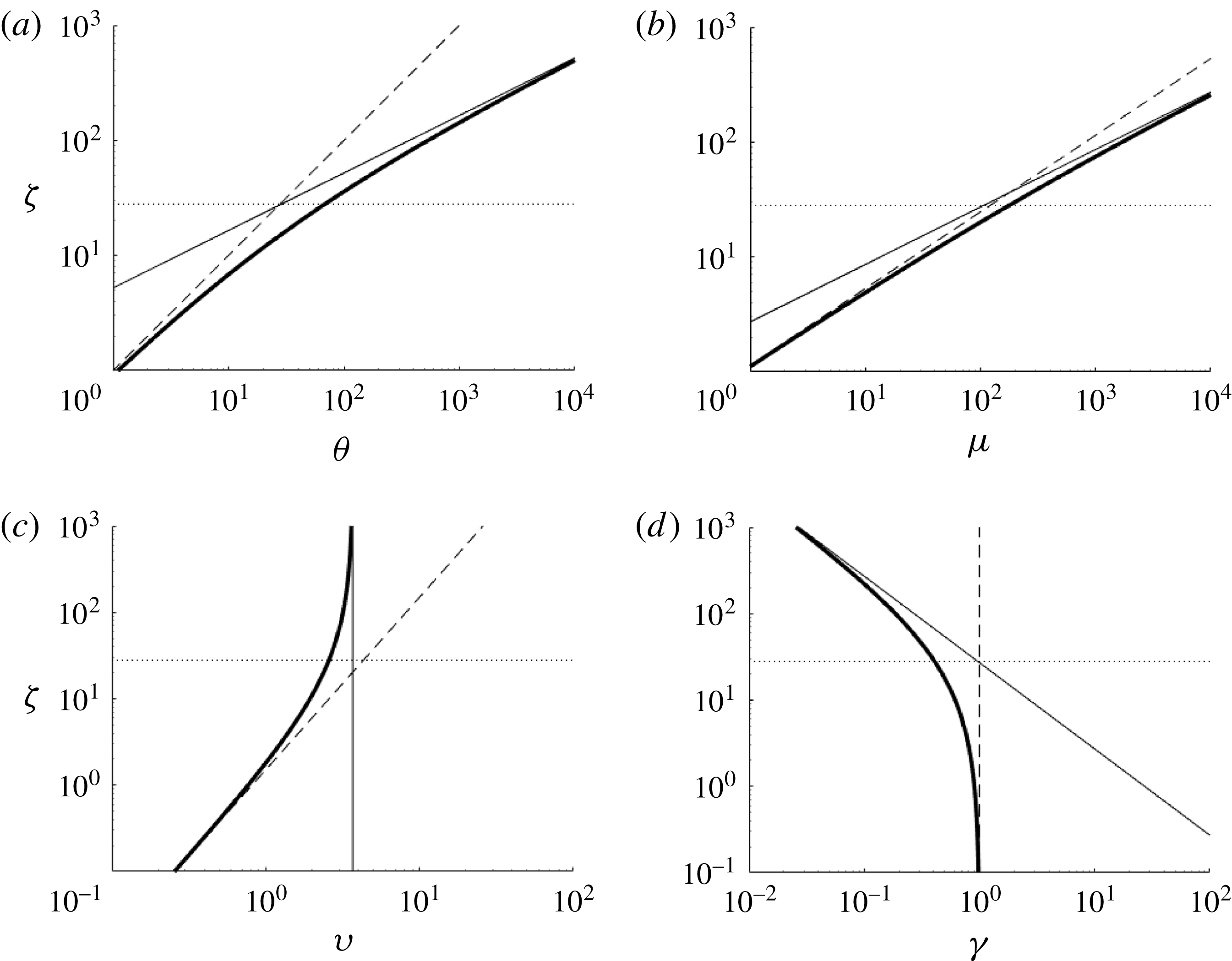
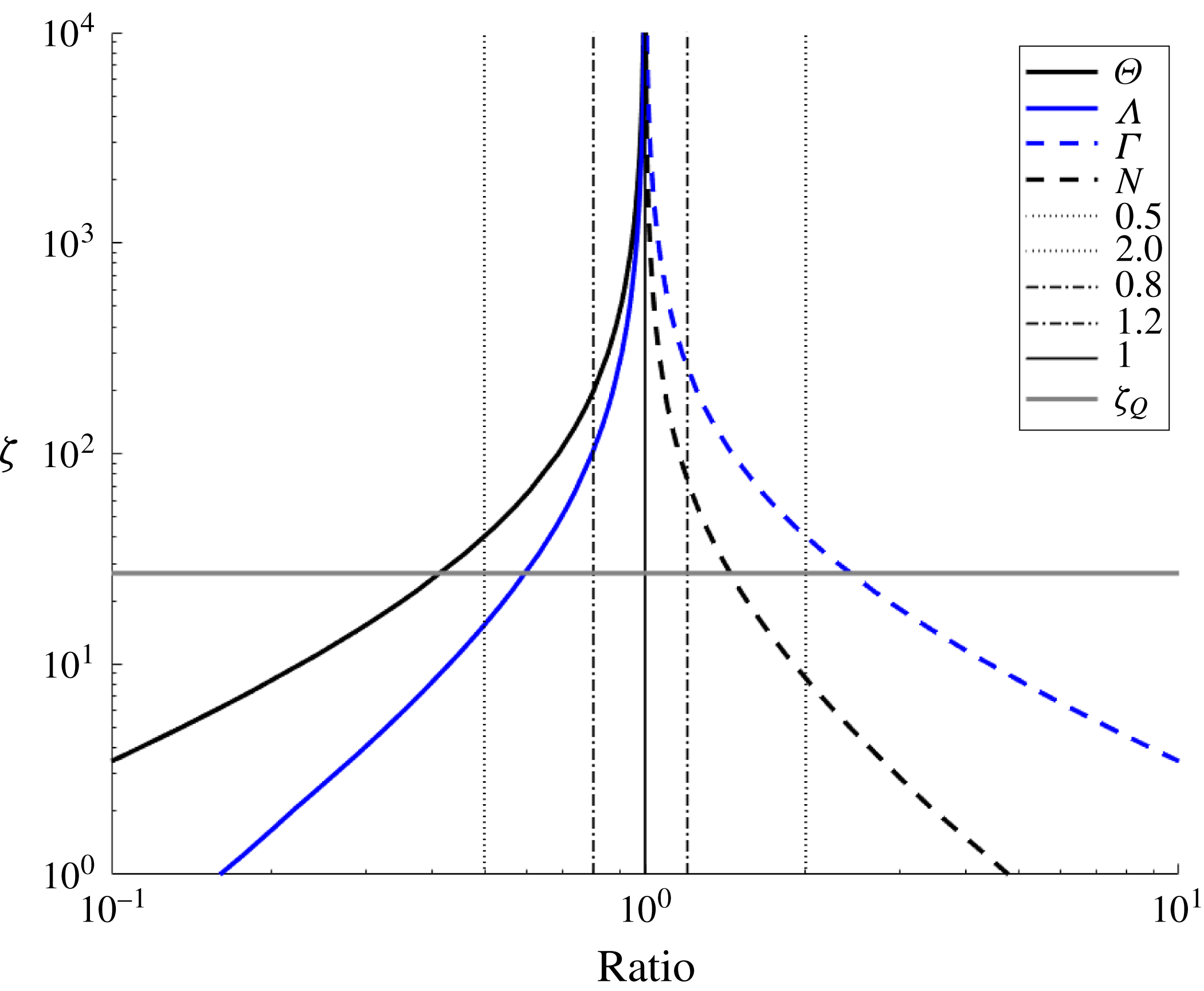
The transition towards the ideal plume solution occurs over a significant distance as shown in figure 10. As with the wall plume, the transition length
 $\unicode[STIX]{x1D701}_{Q}$
underestimates the point at which the plume fluxes are similar. For example, for
 $\unicode[STIX]{x1D6FC}=0.1$
,
 $\unicode[STIX]{x1D701}_{Q}=27$
, at which height the volume and momentum fluxes in a plume with finite source volume flux are, respectively, 2.4 and 1.7 times those of an ideal source plume (compared to 1.73 and 1.35 for the wall plume). This is a much larger disparity than for the wall plume as, in a round plume, the entrainment rate increases less rapidly with height as it is dependent on both the momentum flux and the plume circumference, both of which increase with height, whereas a wall plume has a constant width over which entrainment occurs.
However, as the circumference increases with height, the approach to the pure plume solution becomes more rapid with height compared to a wall plume in which perimeter is constant with height. For example, while the height at which the finite volume flux wall plume volume flux is within 20 % of the pure plume flux is
 $\unicode[STIX]{x1D701}\approx 6\times 10^{3}$
or approximately
 $20\unicode[STIX]{x1D701}_{Q}$
, for a round plume this value is
 $\unicode[STIX]{x1D701}\approx 260$
or approximately
 $9.6\unicode[STIX]{x1D701}_{Q}$
. The buoyancy in the ideal and non-ideal vertical line plumes match to within 20 % when
 $\unicode[STIX]{x1D701}\approx 201$
or approximately
 $7.4\unicode[STIX]{x1D701}_{Q}$
. Therefore, experiments to examine the behaviour of an ideal vertical line plume would need to extend to heights significantly greater than
 $200L_{S}$
(where
 $L_{S}$
is defined in (3.2a
)) in order to avoid the influence of a non-ideal vertical line source on major plume parameters.
Plot of the ratio of the ideal source solution to the finite volume flux solution for the plume volume flux, momentum flux, buoyancy and velocity. The data used are from the same numerical integrations used for figure 9 with the same initial conditions. See (2.18) for definitions of the symbols in the legend.
3.2 Confined vertically distributed round plume
We repeat the filling-box analysis of § 2.2 for the round plume case. The box geometry is similar to that of the wall plume except that the horizontal cross-sectional area of the box (
 $A$
) is used to quantify the horizontal extent of the box rather than the box length normal to the source wall (
 $L=\text{area}/\text{width}$
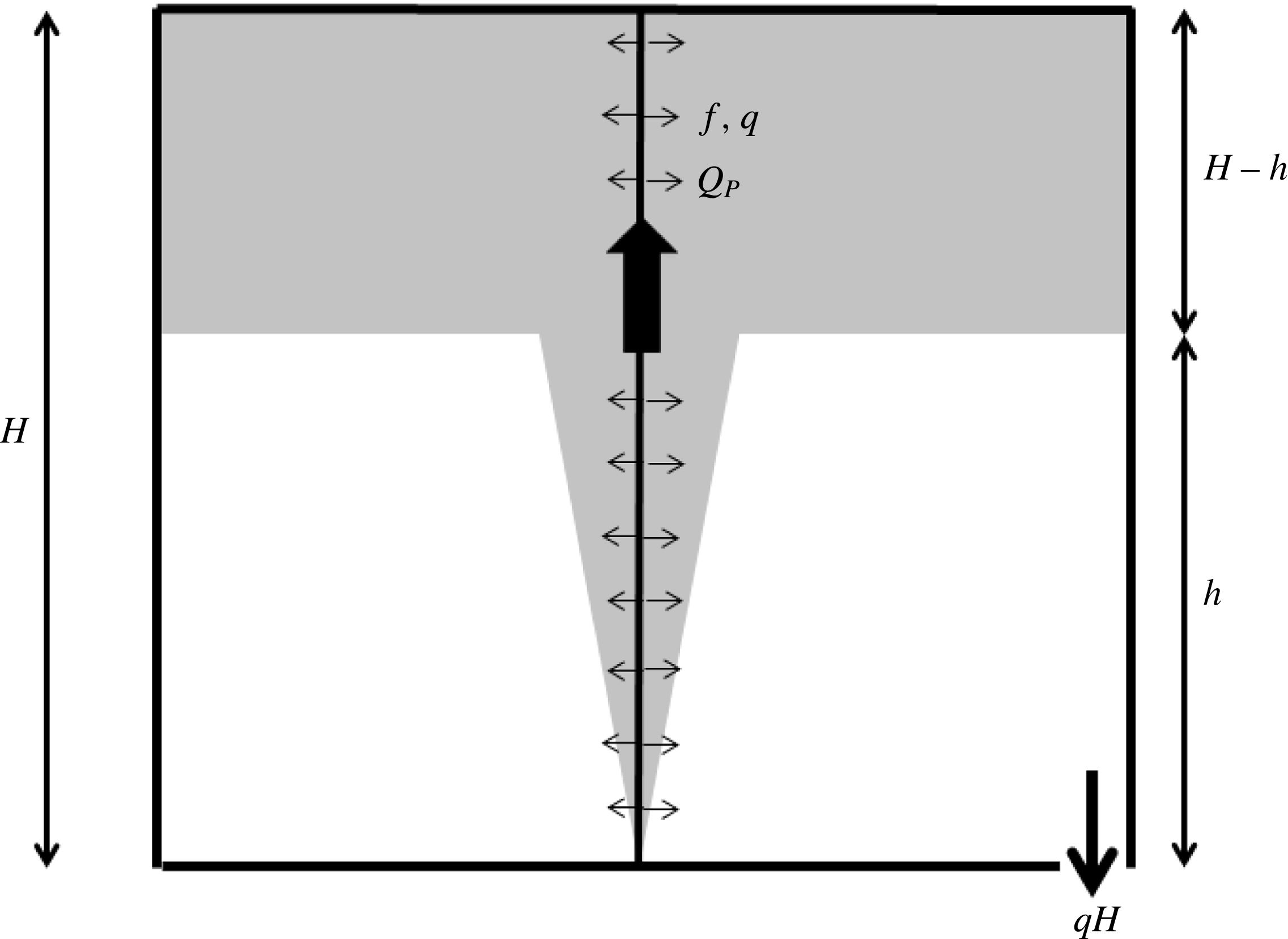
). A schematic diagram of this filling-box flow is shown in figure 11.
Schematic diagram of a confined vertically distributed wall plume showing the wall plume flow and upper buoyant layer that thickens over time as plume fluid is added. The outlet at the base drains a volume flux equivalent to the vertical-line-source volume flux.
Conservation of volume for the upper dense layer combined with the equation (3.8) for the plume volume flux (assumed ideal here) leads to
 $$\begin{eqnarray}\frac{\text{d}h}{\text{d}t}=-\frac{C_{VL}\,\hat{f}^{1/3}h^{2}+q(H-h)}{A}.\end{eqnarray}$$
Using the non-dimensional variables,
 $$\begin{eqnarray}\unicode[STIX]{x1D709}=\frac{h}{H}\quad \text{and}\quad \unicode[STIX]{x1D70F}=\frac{t}{T_{F}}=\frac{H\hat{f}^{1/3}}{A}t,\end{eqnarray}$$
(3.14) can be rewritten as
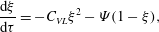 $$\begin{eqnarray}\frac{\text{d}\unicode[STIX]{x1D709}}{\text{d}\unicode[STIX]{x1D70F}}=-C_{VL}\unicode[STIX]{x1D709}^{2}-\unicode[STIX]{x1D6F9}(1-\unicode[STIX]{x1D709}),\end{eqnarray}$$
where
 $\unicode[STIX]{x1D6F9}=L_{s}/H$
is the ratio of the plume source length scale to the box height. Therefore, the assumption of an ideal plume source is only valid provided that
 $\unicode[STIX]{x1D6F9}$
is very small. However, even if
 $\unicode[STIX]{x1D6F9}$
is very small compared to
 $C_{VL}\unicode[STIX]{x1D709}^{2}$
such that the plume behaves as an ideal source plume over the bulk of the box height, there will be a height at which the first front is close enough to the floor that the second term on the right-hand side of (3.16) becomes greater than the first. This height is given by
 $$\begin{eqnarray}\unicode[STIX]{x1D709}_{F}=\frac{\sqrt{\unicode[STIX]{x1D6F9}^{2}+4C_{VL}\unicode[STIX]{x1D6F9}}-\unicode[STIX]{x1D6F9}}{2C_{VL}}.\end{eqnarray}$$
Provided
 $\unicode[STIX]{x1D709}_{F}\ll 1$
, the plume source volume flux above the first front will be relatively small, the second term on the right-hand side of (3.16) can be ignored, and (3.16) can be integrated, subject to
 $\unicode[STIX]{x1D709}=1$
at
 $\unicode[STIX]{x1D70F}=0$
, to give
 $$\begin{eqnarray}\frac{1}{\unicode[STIX]{x1D709}}-1=C_{VL}\unicode[STIX]{x1D70F}.\end{eqnarray}$$
3.3 Impact of source conditions on previously published experimental studies
We examine the impact of a non-ideal plume source (
 $q>0$
) on vertical line plume filling-box measurements using the experiments of GW. The goal of this section is to examine the impact of non-ideal source conditions on the first front movement and subsequent estimation of the vertical line plume entrainment coefficient.
The experiments of GW used a vertical segmented tube with rings of holes around each segment to allow plume fluid to flow out into the ambient. Each tube segment was supplied separately with a known flux of dense plume fluid. The experiments reported were not classic filling-box tests but rather forced emptying filling-box tests. That is, the vertically distributed round plume was released into an enclosure with an imposed flow rate added at the level of the base of the plume and extracted at the level of the top of the plume. This is effectively the same as the Baines (Reference Baines1983) experimental set-up used to measure the volume flux in a plume. In this case the first front will eventually stop when the flow through the interface due to the plume plus the source volume flux above the front balances the imposed ambient flow rate. However, this is simply the filling-box problem with a sink term on the right-hand side of (3.14) to account for the ambient outflow from the buoyant upper layer. This produces a steady version of the filling-box problem with all the other length and time scales unchanged. As with the wall plume experiments, GW observed detrainment from the plume above the first front. This is discussed in § 4.
The experiments of GW were run in a box of height
 $H=0.14{-}0.3~\text{m}$
and area
 $A=0.2025~\text{m}^{2}$
. A total of 26 tests were reported for different box heights and source fluxes. The source volume and buoyancy fluxes per unit height ranged over
 $q=(1.2{-}4.3)\times 10^{-6}~\text{m}^{2}~\text{s}^{-1}$
and
 $f=(0.98{-}6.2)\times 10^{-6}~\text{m}^{3}~\text{s}^{-3}$
, with the source buoyancy ranging over
 $g^{\prime }=0.7{-}1.7~\text{m}~\text{s}^{-2}$
. The source length scale ranged over
 $9.6\times 10^{-5}<L_{s}<2.3\times 10^{-4}~\text{m}$
such that the height at which the plume volume flux would be within 10 % of the equivalent ideal source plume ranged over
 $0.054<L_{90}<0.13~\text{m}$
, which, scaled on the box height, gives
 $0.18<L_{90}/H<0.62$
. The relative height at which the plume source volume flux above the first front equals the ideal plume volume flux at the front height ranged over
 $0.066<\unicode[STIX]{x1D709}_{F}<0.12$
. The reported entrainment coefficient was
 $\unicode[STIX]{x1D6FC}=0.09$
based on a fit through the flow rate versus height data from the Baines (Reference Baines1983) type experiments they conducted.
We consider a typical test (experiment P) from GW with
 $L_{90}/H=0.21$
and
 $\unicode[STIX]{x1D709}_{F}=0.07$
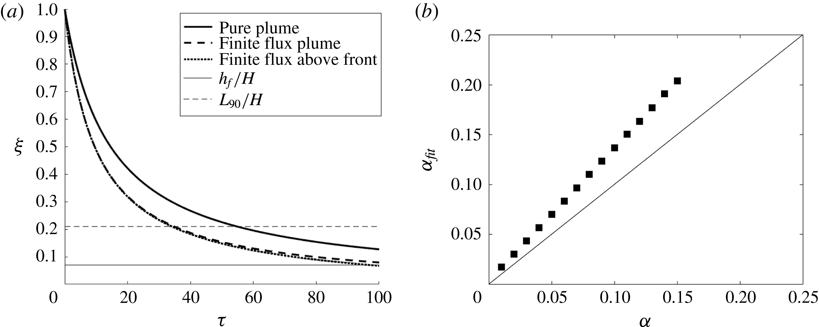
. As with the experiments of BCL and CH, the first front movement was calculated for three different cases. These were (i) the pure plume case given by (3.16), (ii) the finite source volume flux plume but with the volume flux above the front ignored (second term on right-hand side of (3.14)), and (iii) a full simulation in which the source volume flux is included both in the plume calculation and in (3.14). The results of these simulations are plotted in figure 12(a). As with the wall plume examples in figure 6, the inclusion of the source volume flux in the plume equations makes a significant difference to the front position over time. Even though
 $L_{90}/H$
is quite small, the divergence in the front position from the pure plume occurs fairly early in the simulation as small volume flux discrepancies integrated over time lead to large front position differences. In the test considered
 $\unicode[STIX]{x1D709}_{F}$
is very small, so that the plume source volume flux above the front makes very little difference to the front movement with the plotted lines overlapping until
 $\unicode[STIX]{x1D709}<0.2$
.
(a) Plot of the simulated first front from test P of GW for the same set of modelling assumptions as figure 6. The solid line represents the front movement for a pure plume with no source volume flux, the dashed line is for a plume with a source volume flux and the dotted line is for a plume with a source volume flux and in which the volume flux above the first front is included in the front movement equation. (b) Plot of the entrainment coefficient calculated based on a fit through the first front position over time against entrainment coefficient for the experimental conditions used in test P of GW for the case when the source volume flux is included in the plume fluxes but not the filling-box equations. The line represents exact agreement. A line of best fit through the data has a slope of 1.34, indicating that this approach would overestimate the entrainment coefficient by 34 %.

Using the same set of experimental conditions, the first front position for a filling-box experiment was calculated for different values of
 $\unicode[STIX]{x1D6FC}$
in the range 0.01–0.15. As
 $\unicode[STIX]{x1D709}_{F}$
is small for this set of conditions, the plume source volume flux was only included in the plume equations (3.1) and not in the front movement equation (3.14). The non-dimensional front position,
 $\unicode[STIX]{x1D709}$
, was then used to calculate the value of the left-hand side of (3.18). A linear fit to these data versus time was then calculated to establish a fitted value of
 $C$
. This, in turn, was used to calculate the apparent entrainment coefficient for the experiment
 $\unicode[STIX]{x1D6FC}_{fit}$
. This represents the value of
 $\unicode[STIX]{x1D6FC}$
that would have been calculated using a fit through the first front position over time given an actual entrainment coefficient
 $\unicode[STIX]{x1D6FC}$
. A plot of
 $\unicode[STIX]{x1D6FC}_{fit}$
versus
 $\unicode[STIX]{x1D6FC}$
is shown in figure 12(b) (analogous to figure 7 for wall plumes). As with the wall plume experiments, the filling-box front position entrainment coefficient is larger than the plume entrainment coefficient due to the source volume flux producing a plume flow rate greater than that of the ideal plume. For the example considered
 $\unicode[STIX]{x1D6FC}_{fit}$
was 34 % larger than
 $\unicode[STIX]{x1D6FC}$
. This would be typical of the experiments of GW as the values of
 $L_{90}/H=0.21$
and
 $\unicode[STIX]{x1D709}_{F}=0.07$
are close to the average values used. In their experiments
 $L_{90}/H=0.28$
and
 $\unicode[STIX]{x1D709}_{F}=0.08$
. Based on their reported value of
 $\unicode[STIX]{x1D6FC}=0.09$
, based on emptying filling-box measurements, the actual value would be closer to
 $\unicode[STIX]{x1D6FC}=0.07$
. This is smaller than many measurements for round point-source plumes of
 $\unicode[STIX]{x1D6FC}=0.12$
(see Fischer et al.
Reference Fischer, List, Koh, Imberger and Brooks1979). However, this lower value is consistent with the measurements for vertically distributed wall plumes (CH; BCL) that exhibit reduced entrainment relative to line plumes. This point is discussed further in § 4.
3.4 Impact of wall shear stress on a vertical line plume
For a vertical line source of buoyancy the buoyancy force per unit height increases linearly with height whereas the velocity is constant with height. Therefore, assuming that the wall shear stress scales on the velocity squared, as in (2.25), the shear stress on the wall will be constant and will eventually be negligible compared to the buoyancy force and, therefore, will not influence the flow. The calculations presented in § 3.3 suggest that the appropriate entrainment coefficient for the experiments of GW is
 $\unicode[STIX]{x1D6FC}=0.07$
, which is quite a bit smaller than the typical value of
 $\unicode[STIX]{x1D6FC}=0.12$
for a point-source plume (Fischer et al.
Reference Fischer, List, Koh, Imberger and Brooks1979). In this case the discrepancy cannot be attributed even in part to wall shear stresses, which suggests that the source velocity may play a role in reducing entrainment. This point is discussed in the next section.
4 Discussion of source and boundary condition impact on entrainment
Herein we discuss the potential impact of source and boundary conditions on the entrainment and detrainment processes in vertically distributed plumes. The discussion is motivated by two experimental observations that are consistent across the literature on vertically distributed plumes formed by the injection of salt water into a fresh quiescent ambient (CH; BCL; GW). These are as follows.
(1) The entrainment coefficient measured is considerably less than that observed for the equivalent-geometry localized source of buoyancy (horizontal line plume for a wall plume and point-source plume for a vertical line plume).
(2) In filling-box flows, the vertically distributed plumes may lose fluid through detrainment into the stratified environment beyond the first front. This is not observed in plumes with equivalent localized sources of buoyancy.
While these are distinct observations, they may be related as a weaker entrainment process may make the plume more susceptible to detrainment beyond the first front in a filling-box. The following discussion reviews a number of possible explanations for the reduced entrainment coefficient and detrainment observations, and examines how the source and boundary conditions may play a role in these processes. The discussion is mainly focused on wall plumes, as there is a greater body of work on such plumes involving both salt injection techniques (CH; BCL) and other approaches (MK; Caudwell et al. Reference Caudwell, Flór and Negretti2016).
4.1 Reduced entrainment coefficient
There are a number of possible explanations for the reduced entrainment coefficient observed in salt bath experiments. These include (1) reduced momentum due to the presence of wall shear stresses, (2) physical constraint on the growth of the largest eddies and suppression of plume meandering due to the presence of the wall, and (3) the injection of mass and horizontal momentum through the wall source. Each of these possibilities are discussed in turn.
It was shown in § 2.4 that the presence of a wall shear stress will reduce the plume momentum flux at any given height as some of the plume buoyancy force must overcome the wall shear stress and, therefore, is not generating momentum. The net result is that a plume entrainment model that does not account for this wall shear stress will overestimate the plume momentum for a given flow rate and, therefore, underestimate the entrainment coefficient. This almost certainly contributes to the reduced entrainment coefficients observed by CH (
 $\unicode[STIX]{x1D6FC}=0.03$
) and BCL (
 $\unicode[STIX]{x1D6FC}=0.04$
), though it is hard to quantify the extent of the underestimation as there are no shear stress measurements for wall plumes with a convective wall mass flux. Measurements of the entrainment coefficient in plumes with more diffusive boundary conditions such as the ice-melt experiments of MK or the thermal experiments of Caudwell et al. (Reference Caudwell, Flór and Negretti2016) exhibit higher entrainment coefficients. Caudwell et al. (Reference Caudwell, Flór and Negretti2016) and MK report values of
 $\unicode[STIX]{x1D6FC}=0.08$
and
 $\unicode[STIX]{x1D6FC}=0.048$
, respectively. Nevertheless, these are still less than reported entrainment coefficients for a planar horizontal line plume of
 $\unicode[STIX]{x1D6FC}=0.1$
(Paillat & Kaminski Reference Paillat and Kaminski2014).
The presence of the wall along the source of a wall plume provides a physical barrier that constrains the growth of eddies compared to the equivalent horizontal-line-source planar plume. This may reduce the rate of engulfment of ambient fluid into the plume. However, the eddies are predominantly generated by shear and baroclinic torque (Kaye Reference Kaye2008), which are driven by the respective velocity and buoyancy gradients across the width of the plume. This implies that there is no significant driver to produce eddies significantly larger than the plume half-width regardless of the presence or not of the wall. Further, this barrier will have a significantly smaller role in vertical line plumes where similar reductions in
 $\unicode[STIX]{x1D6FC}$
are observed. The suppression of plume meandering by the wall is a more complex problem. Free plumes are observed to meander about their mean centreline or plane of symmetry. This meandering will clearly increase the mean radial extent of the plume at any given height, though it is not obvious that it will induce additional mixing with ambient fluid. A review of experimental measurements of entrainment coefficients for point-source plumes by Kaye & Linden (Reference Kaye and Linden2004) indicated that entrainment coefficients calculated using the radial spread of the plume were larger (
 $\unicode[STIX]{x1D6FC}=0.14$
) than those entrainment coefficients calculated using volume flow rate measurements (
 $\unicode[STIX]{x1D6FC}=0.12$
). This suggests that plume meandering is likely to widen the plume but does not increase the rate of entrainment. This was confirmed by Hubner (Reference Hubner2004), who measured the radial extent of plume meandering and showed that, if the meandering contribution to the radial growth of the plume was subtracted from the total radial growth, then the entrainment coefficient calculated from the volume flux and from the radial growth rate matched. Therefore, it is unlikely that the suppression of wall plume meandering due to the presence of the wall will significantly reduce the plume entrainment coefficient.
Finally, it is possible that the outlet velocity of the wall source overwhelms, or in some way interferes with or suppresses, the entrainment process. The mean plume velocity,
 $u$
, decreases with height in a point-source plume and is constant for a horizontal line plume. In vertically distributed plumes the velocity is constant in a vertical line plume and increases with height in a wall plume. Therefore, for a wall plume with a finite source volume flux there will be a height, denoted by
 $Z_{e}$
, below which the velocity of the source will be greater than the entrainment velocity of the plume,
 $\unicode[STIX]{x1D6FC}u$
. In this region the horizontal source momentum flux may interfere with the entrainment process, suppressing the inflow of ambient fluid. For a vertical line plume the ratio of the source velocity to entrainment velocity will be constant with height, assuming a uniformly distributed vertical source and a fully developed plume.
The conditions under which the source velocity is greater than or equal to the entrainment velocity in the experiments discussed above are summarized in table 3. The calculations used to derive the values in table 3 are based on the experimental descriptions in the papers and the quoted entrainment coefficients for those experiments (see tables 1 and 2). Two ranges for
 $Z_{e}/H$
are quoted for the experiments of BCL and CH based on the average source velocity (
 $q$
) and the physical source exit velocity from the discrete tubes used to create the wall plume in BCL and the pore velocity in the experiments of CH.
Summary of conditions under which the plume source velocity exceeds the plume entrainment velocity. The entrainment velocity is calculated assuming ideal plume flow (equations (2.6c ) and (3.5c )) and the quoted entrainment coefficient from each paper.
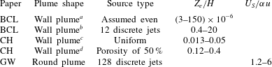
a Calculation based on source volume flux being uniformly distributed over the entire wall.
b Calculation based on exit velocity from the source tubes and assuming a tube diameter of 10 mm (unstated in the paper, but the largest tubes that fit the pump described).
c Calculation made assuming a uniformly distributed source volume flux.
d Calculation made using an estimated outlet pore velocity based on a typical porous PTFE porosity of 50 %.
Of the 20 experiments run by BCL, 17 have the wall-source velocity greater than the entrainment velocity over the entire height of their box, suggesting that there may be regions near the discrete wall-source outlets where the entrainment process may be overwhelmed by the plume source velocity. This is less true for the experiments of CH where the entrainment velocity is greater than the wall-source velocity for between 60 % and 90 % of the box height based on the exit pore velocity from the porous polytetrafluoroethylene (PTFE) plate. The round plume tests of GW always have a source velocity greater than the idealized entrainment velocity despite using 128 discrete inlets in their plume source. It is, therefore, likely that the source horizontal momentum injected into these vertically distributed plumes will inhibit or interfere with the entrainment process, reducing the entrainment coefficient of the plume.
In summary, there are a number of possible causes for the reduced entrainment coefficient measured in vertically distributed plumes relative to their equivalent constant buoyancy flux plumes. While it is likely that the physical constraint on the lateral growth and meandering presented by the presence of a wall will contribute to this reduction, this does not explain the reduction in
 $\unicode[STIX]{x1D6FC}$
for vertical line plumes. The presence of a wall shear stress will reduce the entrainment rate into a wall plume but it is less clear that it will reduce
 $\unicode[STIX]{x1D6FC}$
. The injection of horizontal momentum of a similar scale as the entrainment inflow may well contribute to reducing
 $\unicode[STIX]{x1D6FC}$
and may explain why entrainment coefficient measurements in salt bath plumes (where there is significant horizontal momentum injection) are lower than in the equivalent thermal and ice-melt measurements.
4.2 Plume fluid detrainment
The flow description that has been used most frequently to explain this partial detrainment is the ‘peeling plume’ model. This model is based on the observation that, because the plume has decreasing buoyancy with increasing distance from the wall or line source, there will be some distance from the plume centre at which the local plume buoyancy is less than the ambient buoyancy after the plume crosses the density interface. Therefore, there is a local rather than global buoyancy reversal that drives outer plume fluid to detach from the plume and enter the ambient stratification. See for example figures 1 and 4 of GW and the peeling plume models of BCL, Cortes et al. (Reference Cortes, Rueda and Wells2014) and Hogg et al. (Reference Hogg, Dalziel, Huppert and Imberger2017).
Although this explanation makes physical sense and can be used to develop models for the stratification that match experiments (see BCL), it is not a sufficient criterion for detrainment. Local buoyancy reversal also occurs in point-source plumes in ventilated enclosures (Linden et al. Reference Linden, Lane-Serff and Smeed1990) with no observations of plume peeling recorded in the literature. This observation raises the question: Why is this detrainment seen in vertically distributed plumes but not evident in constant buoyancy flux plumes in a stratified environment when the same local buoyancy flux reversal occurs without detrainment? (Detrainment is observed in point-source plumes in a stratified environment only once the plume has passed the neutral height, that is, once total buoyancy reversal has occurred.) In particular, is this detrainment either influenced by, or even an artefact of, the use of finite volume flux salt plumes in the vertically distributed plume experiments discussed above (CH; BCL; GW)? Three possible mechanisms could lead to the finite source mass flux used in salt bath plumes driving detrainment, namely:
(a) the buoyancy of the fluid at the vertically distributed source is greater than would be expected assuming a self-similar plume buoyancy profile, which in turn results in much larger lateral buoyancy gradients, more buoyant fluid spreading out at the top of the box and a stronger stratification in the filling box;
(b) the finite inflow velocity from the source volume flux drives detrainment; and/or
(c) the stronger horizontal gradients of velocity and buoyancy within the plume make the outer edges more susceptible to detrainment in regions of local buoyancy reversal.
The first possibility is that source fluid is being added to the plume centreline that is significantly more buoyant than the mean plume fluid (see figure 3 d). When this more buoyant fluid spreads out at the top of the box, it will create a buoyancy stratification in the ambient that will be stronger than that produced by an ideal source of pure buoyancy. For example, the source fluid supplied in the experiments of BCL was an order of magnitude more buoyant than that of the equivalent ideal plume at the top of the enclosure. The late-stage density profiles measured by BCL do have larger buoyancy at the top of the enclosure compared to the ideal filling-box model predictions by approximately 25–50 % (figure 9 of BCL). However, this difference is substantially less than would be measured if the wall-source fluid had not partially mixed with the other plume fluid as it spread out at the top of the enclosure. This underprediction of the measured buoyancy at the top of the box is not observed in the stratification measurements of the line plume that exhibit very small differences between measurement and model at larger times (figure 6 of BCL). However, the difference between the measured and modelled enclosure buoyancy profiles were not observed across the entire profile, rather only at the profile top where the plume spread out. That is, the fact that the wall-source buoyancy was significantly greater than the mean plume buoyancy at the top of the enclosure did not significantly alter the enclosure stratification over most of the enclosure height and, therefore, it is unlikely that the wall-source fluid buoyancy contributes significantly to creating a stratification that induces peeling.
The impact of the wall-source velocity on the entrainment process was discussed in § 4.1, where it was shown that, for the vertically distributed plume experiments in the literature that used salt water injection for their plume source, the majority of the experiments used injection velocities that were equal to or greater than the entrainment velocity of the plume. Having the source velocity exceed the entrainment velocity at any given height does not necessarily mean that the entrainment process has broken down and the plume will peel. The individual source jets will rapidly entrain plume fluid, slow down and be swept upwards by the plume (though the horizontal momentum flux will be conserved). Furthermore, in the experiments described above, peeling and detrainment are only observed above the density interface in the stratified portion of the enclosure. This suggests that perhaps a combination of the source momentum flux interfering with or suppressing entrainment combined with local buoyancy reversal may make the outer regions of the plume more susceptible to the peeling process.
The third possibility is that the stronger horizontal gradients of buoyancy and/or velocity observed in vertically distributed plumes compared to constant buoyancy flux plumes means that the local buoyancy reversal will be greater. This, in turn, may make them more susceptible to detrainment than constant buoyancy flux plumes are. This would be consistent with the observations of Baines (Reference Baines2005) for plumes flowing down a slope where there is a lower stable layer overlaid with a more diffuse upper layer that mixes with the ambient and may ultimately detrain. The introduction of dense fluid at the wall will, as discussed above, lead to a higher peak buoyancy in the plume profile. Velocity profiles measured in wall plumes have also shown a thin region of high velocity with a slower outer region. If both the buoyancy and velocity profiles have higher peaks and thinner tails compared to the free plume equivalent profile, then buoyancy reversal will be more extensive and the vertical momentum in the region of buoyancy reversal will be less than for plumes from localized sources of buoyancy. This would induce detrainment not only in the salt bath plumes but also in the thermal (Caudwell et al. Reference Caudwell, Flór and Negretti2016) and ice-melt (MK) plumes which also exhibited detrainment or exchange flows between the plume and the surrounding ambient fluid. Further, the experiments of Caudwell et al. (Reference Caudwell, Flór and Negretti2016) indicated that the entrainment coefficient reduced over time as the enclosure became more strongly stratified. The stronger stratification will lead to stronger local buoyancy reversal as the plume fluid passes into increasingly buoyant fluid leading to a great propensity for fluid packets to detrain from the plume, thus reducing the net inflow of ambient fluid into the plume and the time-averaged entrainment coefficient. The increasing stratification will also reduce the net buoyancy of the plume reducing the potential for buoyancy-induced overturning and mixing with the ambient (see Kaye Reference Kaye2008).
5 Conclusions
Vertically distributed plumes, that is, wall and vertical line plumes, formed by the injection of buoyant fluid at the buoyancy source will result in source effects at all heights in the plume. Near the base of the plume the flow rate in the plume will be dominated by the source volume flux. Further up the plume the buoyancy of the fluid injected will be substantially more buoyant than the equivalent pure plume buoyancy leading to larger buoyancy gradients across the plume width. The presence of source effects at all heights is fundamentally different from that of the equivalent constant buoyancy flux plumes (horizontal line and point-source plumes). For constant buoyancy flux plumes the non-ideal nature of the plume resulting from a source mass flux can be accounted for using a virtual origin correction (Hunt & Kaye Reference Hunt and Kaye2001) and the plume approaches an ideal plume (pure plume) at large distances from the source.
The use of a finite source of mass and buoyancy distributed vertically, whether along a line (GW) or across a plane (CH; BCL), will influence the development of the stratification within a filling box. If the mass flux is too large (
 $L_{S,W}/H\sim O(1)$
) then the plume will not behave as a pure plume over the height of the enclosure. Further, the mass flux added to the plume above the first front will result in the upper buoyant layer thickening more rapidly than predicted. This can lead to a miscalculation of the resulting entrainment coefficient for the plume, as the additional mass flux in the plume, due to the source volume flux both above and below the first front, is included in the entrained mass calculation (see figures 7 and 12
b). If the source mass flux is kept low, such that
 $L_{S,W}/H\ll 1$
, this problem is less significant.
However, a second difficulty then arises in that, for much of the plume height, the source fluid buoyancy is much greater than the mean plume buoyancy. For example, in the experiments of BCL, the plume source fluid density is 14–50 times the modelled mean plume density at the top of the plume. Although the plume buoyancy averaged across the whole plume width is likely to be as modelled, the horizontal distribution of buoyancy within the plume will have much greater gradients than a typical self-similar Gaussian profile, often assumed in the literature.
The use of a finite mass flux at the source may also alter the velocity distribution within the plume. The ice melt plume of MK exhibited high velocity gradients with a peak velocity very close to the wall. Their calculations indicated that of the order of 90 % of the buoyancy force is required to overcome the wall shear stress and, therefore, the average plume velocity is much less than that predicted by models that ignore this shear. This meant that the plume entrainment coefficient they calculate by direct measurement of the velocity profiles is much higher than predicted by tracking the first front movement and ignoring wall shear stress losses. The inclusion of a turbulent wall shear stress in the plume equations does not however alter the power-law behaviour of the plume parameters. It is, however, possible that both the salt and ice techniques calculate accurate entrainment coefficients and that the difference in the measurement is because the entrainment process differs between plumes generated by the two methods. As MK point out, salt plume experiments have a convective wall source whereas the ice wall experiments have a predominantly diffusive wall source with some convection due to melt water release. Therefore, it is conceivable that salt plume experiments have much lower wall shear stress compared to the experiments of MK and that the mass flux injection process inhibits the plume entrainment process.
It is clear that, unlike point-source or horizontal-line-source plumes, source effects in vertically distributed finite volume flux plumes exist at all heights. Either the source volume flux exceeds the entrainment volume flux and/or the source buoyancy exceeds the plume buoyancy. This can lead to more rapid first-front movement in a filling box or the development of stratifications that are stronger than predicted. Additional complications arise when discrete plume sources are used, as the outlet velocity may exceed the entrainment velocity of the plume. It is not clear that all these issues can be avoided in a given experimental set-up, particularly given the difficulty of generating evenly distributed plume sources. It is, therefore, perhaps a problem that more lends itself to computational analysis where zero volume flux source conditions could be examined with high-resolution flow visualization.