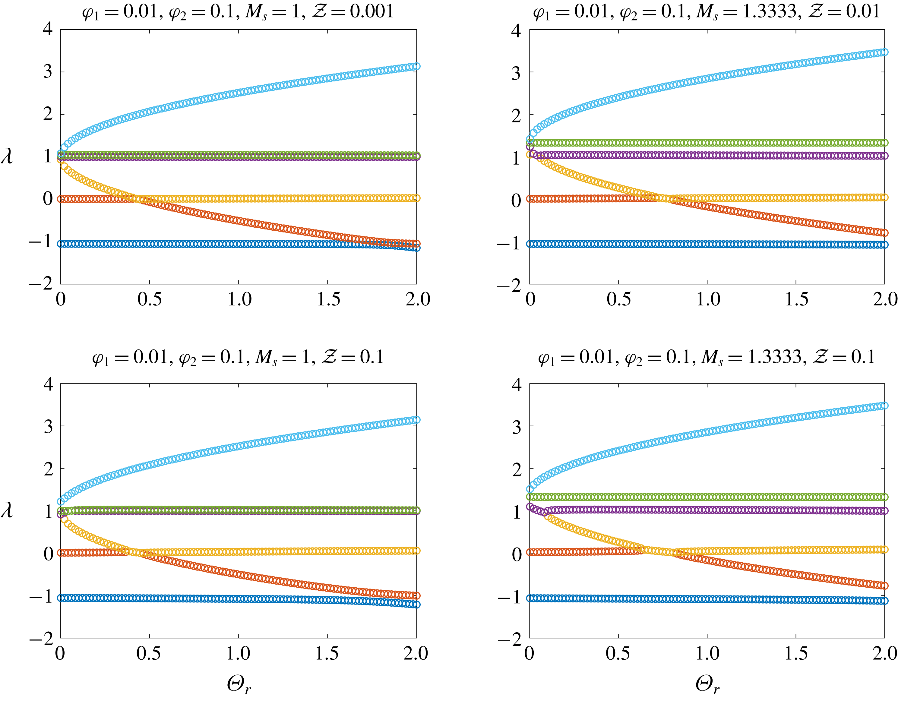
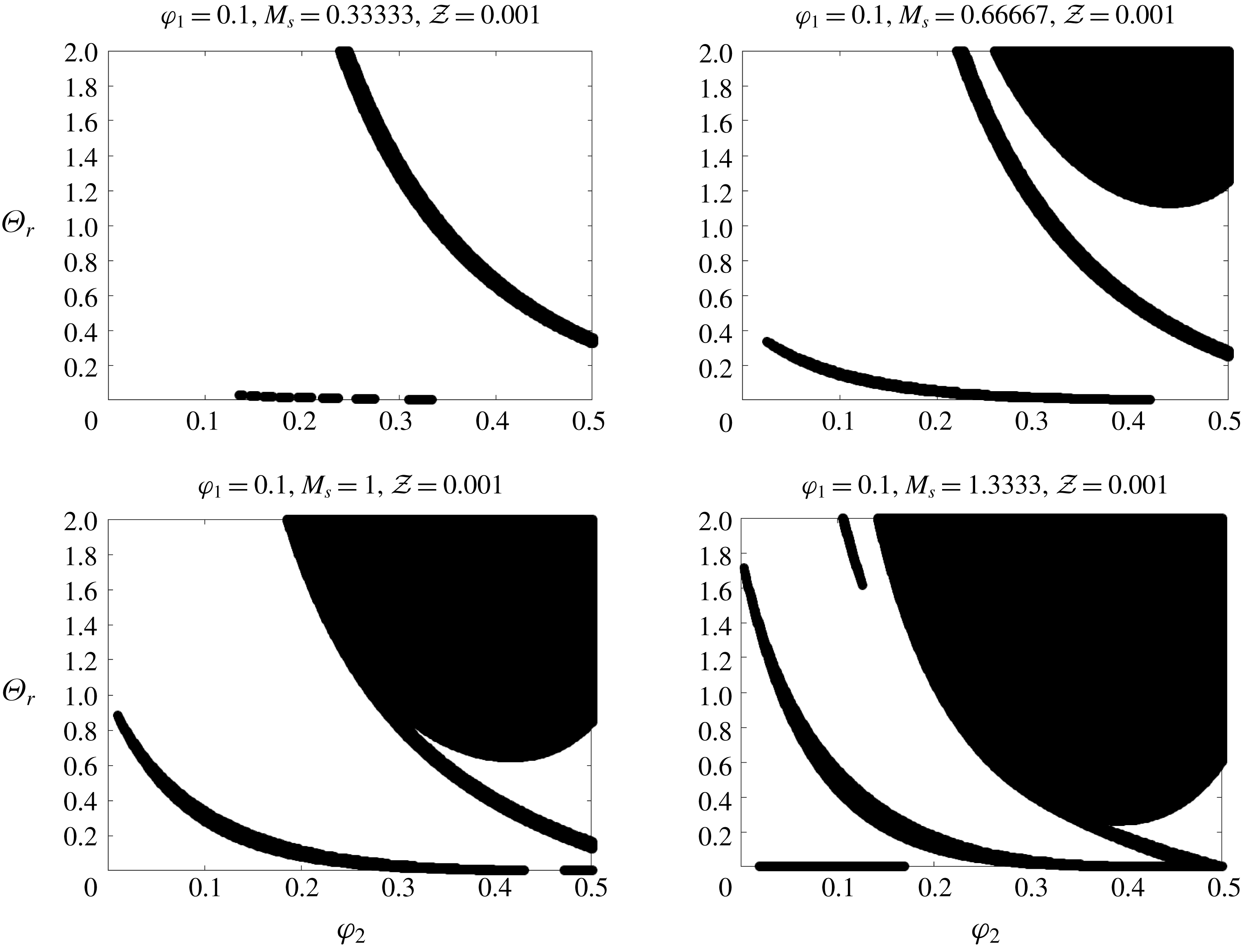
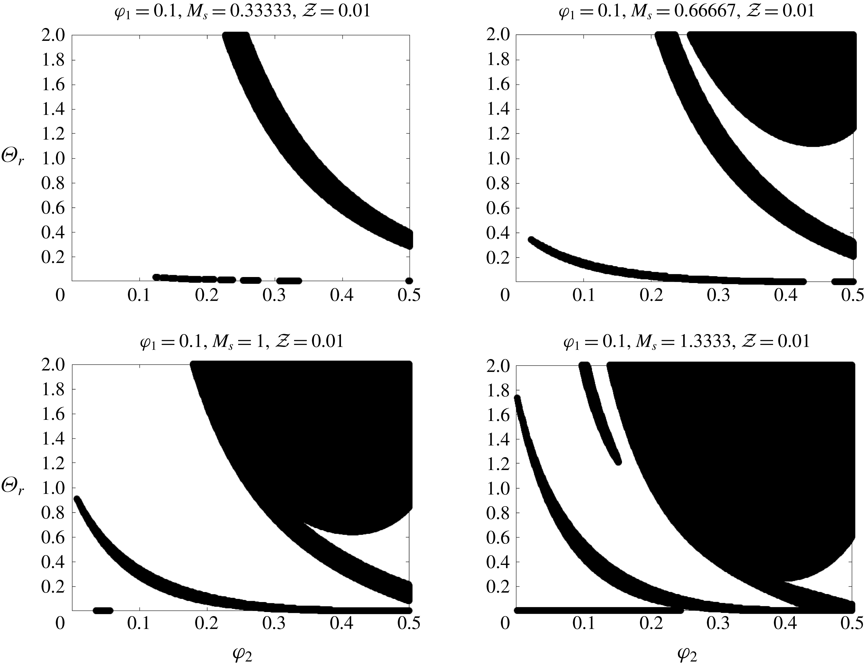
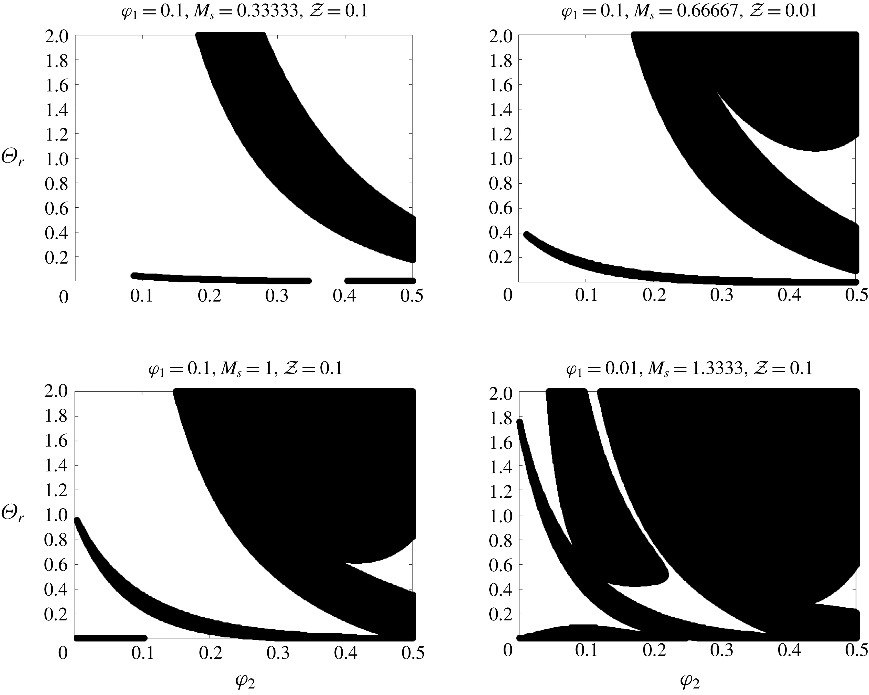
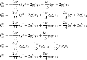
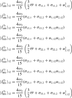
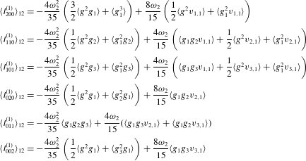
1 Introduction
The long history, and numerous difficulties, of the development of hyperbolic two-fluid models for disperse multiphase systems has been reviewed by Lhuillier, Chang & Theofanous (Reference Lhuillier, Chang and Theofanous2013). These authors note that most, if not all, of the models that have been proposed in the literature suffer from being mathematically ill posed (see Drew & Passman (Reference Drew and Passman1998), Vazquez-Gonzalez, Llor & Fochesato (Reference Vazquez-Gonzalez, Llor and Fochesato2016) for other discussions of this topic). Moreover, well posedness of nonlinear multiphase flow models implies hyperbolicity of the underlying Cauchy problem (Métivier Reference Métivier2005). In practice, numerical simulations with non-hyperbolic two-fluid models diverge under grid refinement due to the complex eigenvalues in the continuum limit (see, e.g. Ndjinga Reference Ndjinga2007; Kumbaro & Ndjinga Reference Kumbaro and Ndjinga2011). To remediate this problem, various ad hoc correction terms have been added to make the models well posed (see, e.g. Panicker, Passalacqua & Fox Reference Panicker, Passalacqua and Fox2018), albeit with dubious physical justification (Lhuillier et al. Reference Lhuillier, Chang and Theofanous2013). In particular, many authors have resorted to neglecting the Archimedes force (see, e.g. Hank, Saurel & Le Metayer Reference Hank, Saurel and Le Metayer2011), which is the root cause of non-hyperbolicity. In their review, Lhuillier et al. (Reference Lhuillier, Chang and Theofanous2013) demonstrate that (i) it is critical to account for the kinetic energies of each phase and (ii) the hyperbolicity is linked to the relation between the forces and stresses (referred to hereinafter as the spatial fluxes) in the momentum and energy balances. In the context of this work, the two-fluid modelling described in Lhuillier et al. (Reference Lhuillier, Chang and Theofanous2013) is done at the macroscopic level. In other words, the forces and fluxes are added at the level of the mass, momentum and energy balances without an underlying microscale model. Related approaches have been used by many other authors (see, e.g. Buyevich & Shchelchkova Reference Buyevich and Shchelchkova1978; Nigmatulin Reference Nigmatulin1979; Jackson Reference Jackson1997; Lhuillier & Theofanous Reference Lhuillier, Theofanous and Cacuci2010; McGrath II, St. Clair & Balachandar Reference McGrath II, St. Clair and Balachandar2016; Saurel, Chinnayya & Carmouze Reference Saurel, Chinnayya and Carmouze2017).
Similar to the kinetic-based approach used in this work, the works of Zhang & Prosperetti (Reference Zhang and Prosperetti1994) and Zhang, Ma & Rauenzahn (Reference Zhang, Ma and Rauenzahn2006) treat the particle phase using a kinetic description in terms of the
 $N$
-particle distribution function. In Zhang & Prosperetti (Reference Zhang and Prosperetti1994), the particles evolve in an Euler fluid and averaged equations are derived for the mass and momentum of each phase. These authors demonstrate that interphase momentum interactions due to the fluid pressure at the particle surfaces generates an additional stress tensor (
 $\unicode[STIX]{x1D64F}_{C}$
in their notation, see (10.9) in their article) in the fluid-phase momentum balance. In Zhang et al. (Reference Zhang, Ma and Rauenzahn2006), the
 $N$
-particle distribution function for a dense, binary particulate system is employed to derive the averaged equations for mass and momentum, and the interspecies stress tensor
 $\unicode[STIX]{x1D748}^{(21)}$
is shown to arise from the binary interaction forces between particles of different types. By choosing a specific interaction force (i.e. binary hard-sphere collisions), in the present work explicit expressions are derived for the intra- and interspecies stress tensors and interaction forces in the momentum balances. In addition, closed forms for the total energy equations for each particulate type are derived, allowing us to investigate the hyperbolicity of the resulting two-fluid model. Here, the interaction force is specified to be hard-sphere collisions, allowing us to derive closed expressions for the inter- and intra-species stress tensors, as well as the total energy equations for each species. Because binary hard-sphere collisions are a particular form of binary interactions, the mass and momentum balances derived in the present work have the same structure as in Zhang et al. (Reference Zhang, Ma and Rauenzahn2006). Most notably the momentum equations contain an interspecies stress tensor that plays a significant role is the hyperbolicity of the system.
Given the difficulties described in Lhuillier et al. (Reference Lhuillier, Chang and Theofanous2013) that are faced when formulating a generic two-fluid model for disperse multiphase systems, it would seem judicious to first derive a model for a specific system starting from a microscale description with simple, well-defined physics. Such a system is a binary mixture of elastic hard spheres with dissimilar properties, which has been widely analysed in the context of the kinetic theory of gas dynamics (Enskog Reference Enskog1911a ,Reference Enskog b ; Chapman Reference Chapman1912; Chapman & Cowling Reference Chapman and Cowling1952; Kolodner Reference Kolodner1957; Sirovich Reference Sirovich1962; Morse Reference Morse1963; Hamel Reference Hamel1966; Goldman & Sirovich Reference Goldman and Sirovich1967; Barajas, Garcia-Colin & Pinã Reference Barajas, Garcia-Colin and Pinã1973; Santos, Yuste & López de Haro Reference Santos, Yuste and López de Haro1999). Starting from the Boltzmann–Enskog (BE) kinetic equations for a binary system, the principal objective of this work is to derive a two-fluid model for the mass, momentum and kinetic energy of each phase for a hard-sphere mixture that includes the Archimedes force, as well as other forces depending on spatial gradients (e.g. lift). Then, by going to the limit where the volume and mass for type-1 particles is very much smaller than for type-2 particles, we wish to develop a two-fluid model for fully compressible fluid–particle flow wherein all of the fluxes and forces are derived exactly from the microscale description. (The two-fluid model is compressible in the sense that each phase is governed by the gas-dynamic equations for mass, momentum and energy in the absence of the other phase.) The main limitation of this approach is that it accounts only for spatial gradients up to first order (Barajas et al. Reference Barajas, Garcia-Colin and Pinã1973); however, this is exactly what is required for the spatial fluxes and the Archimedes force. Note that unlike in the ‘classical’ kinetic theory for gas dynamics (see, e.g. Sirovich Reference Sirovich1962; Hamel Reference Hamel1966), in the context of two-fluid models we do not make use the Chapman–Enskog expansion (Chapman & Cowling Reference Chapman and Cowling1952; Garzó, Dufty & Hrenya Reference Garzó, Dufty and Hrenya2007) about the system’s mean velocity and temperature. Instead, the two-fluid model is written in terms of the velocity moments for each phase up to second order for a non-dissipative system. Remarkably, we shall see that the terms in the two-fluid model that determine whether the system is hyperbolic can all be expressed in closed form, thereby removing any ambiguity in the definition of the model. Thus, while the application of the two-fluid model derived in this work is limited to a specific system (i.e. binary, hard-sphere mixture), it should be possible to arrive at some general conclusions concerning the relationship between the fluxes and forces in hyperbolic two-fluid models. As noted above, our results for the mathematical form of the momentum equations agree with Zhang et al. (Reference Zhang, Ma and Rauenzahn2006) whose derivation is based on a Liouville equation for dense binary mixtures with an interaction force between particles.
Starting with the seminal work of Cravath (Reference Cravath1930), many authors have investigated the kinetic theory of molecular-scale hard spheres with disparate masses (e.g. Kolodner Reference Kolodner1957; Sirovich Reference Sirovich1962, Reference Sirovich1963; Morse Reference Morse1963, Reference Morse1964; Hamel Reference Hamel1965, Reference Hamel1966; Goldman & Sirovich Reference Goldman and Sirovich1967, Reference Goldman and Sirovich1969). In these works, the Boltzmann collision operator (i.e. neglecting two-particle correlations) is applied to binary systems with nearly equal mole fractions (such as in a plasma). The primary focus of these works is to investigate the epochal-relaxation scenario introduced by Grad (Reference Grad and Devienne1960). Denoting the mean velocity of each species by
 $\boldsymbol{u}_{\unicode[STIX]{x1D6FC}}$
and the temperature by
 $\unicode[STIX]{x1D6E9}_{\unicode[STIX]{x1D6FC}}$
(see § 2 for details), in a binary system at equilibrium
 $\boldsymbol{u}_{1}=\boldsymbol{u}_{2}$
and
 $m_{1}\unicode[STIX]{x1D6E9}_{1}=m_{2}\unicode[STIX]{x1D6E9}_{2}$
, where
 $m_{\unicode[STIX]{x1D6FC}}$
is the species mass. Epochal relaxation towards this equilibrium applies when
 $m_{1}\ll m_{2}$
(see, e.g. Morse Reference Morse1963), and predicts that the ‘diffusion velocity’
 $|\boldsymbol{u}_{12}|=|\boldsymbol{u}_{1}-\boldsymbol{u}_{2}|$
approaches zero much faster than the temperature difference
 $|m_{1}\unicode[STIX]{x1D6E9}_{1}-m_{2}\unicode[STIX]{x1D6E9}_{2}|$
. In practice, this implies that the mixture can be described by one momentum and two energy equations (i.e. the well-known two-temperature model for plasmas) (Sirovich Reference Sirovich1962; Morse Reference Morse1963; Hamel Reference Hamel1965). For hard-sphere collisions, Morse (Reference Morse1963) introduced a ‘diffusion’ Mach number
 $M_{d}=|\boldsymbol{u}_{12}|/\sqrt{\unicode[STIX]{x1D6E9}_{1}+\unicode[STIX]{x1D6E9}_{2}}$
and derived the relaxation time scales valid for spatially homogeneous systems with
 $M_{d}<0.32$
. In subsequent work on spatially inhomogeneous systems, Hamel (Reference Hamel1966) distinguished between an equal-molar mixture and a system in which the heavy species is a trace component (i.e. when its mole fraction is negligible). The latter occurs, for example, when the diameters
 $d_{\unicode[STIX]{x1D6FC}}$
are related by
 $d_{1}\ll d_{2}$
(which is the case considered in this work). For such cases, Hamel (Reference Hamel1966) demonstrated that epochal relaxation does not occur and, hence, two momentum equations are needed to describe the binary system. In summary, the works of Hamel (Reference Hamel1966) and Goldman & Sirovich (Reference Goldman and Sirovich1967) were the first complete kinetic-based derivations of a two-fluid model for gas mixtures. Interestingly, not much use has been made of these models in the gas-dynamics or granular flow literature. For the former, most practical system have
 $M_{d}\ll 1$
so that the ‘diffusion velocity’ can be replaced with a gradient-diffusion model. For the latter, the Boltzmann collision operator must be replaced by a BE kinetic model to account for the finite size of the particles. As we shall see in § 3, the BE collision model modifies both the relaxation time scales towards equilibrium and the spatial fluxes (and, hence, the hyperbolicity) of the two-fluid model.
For gas–particle flows with heavy particles (e.g. Sinclair & Jackson Reference Sinclair and Jackson1989; Wagner et al. Reference Wagner, Beresh, Kearney, Trott, Castaneda, Pruett and Bear2012), the dominant exchange term is drag (Maxey Reference Maxey2017) (see, e.g. Capecelatro, Desjardins & Fox Reference Capecelatro, Desjardins and Fox2016a , for an analysis of the relative magnitudes of the different forces). Nonetheless, the Archimedes (or buoyancy) force is included in Euler–Lagrange (EL) simulations (Capecelatro & Desjardins Reference Capecelatro and Desjardins2013). The coupling of the Lagrangian particles with the Eulerian fluid is done with a filter that smooths out the small scales of the order of the particle diameter. This explicit filtering will likely eliminate any small-scale instabilities present in non-hyperbolic two-fluid models (Ndjinga Reference Ndjinga2007; Kumbaro & Ndjinga Reference Kumbaro and Ndjinga2011; Panicker et al. Reference Panicker, Passalacqua and Fox2018). From EL simulations, it has been found that the particle-phase granular temperature is significant due to two-way coupling (Capecelatro, Desjardins & Fox Reference Capecelatro, Desjardins and Fox2015; Capecelatro et al. Reference Capecelatro, Desjardins and Fox2016a ; Capecelatro, Desjardins & Fox Reference Capecelatro, Desjardins and Fox2016b ) and/or boundary conditions (Vié, Doisneau & Massot Reference Vié, Doisneau and Massot2015; Chalons et al. Reference Chalons, Fox, Laurent, Massot and Vié2017; Fox, Laurent & Vié Reference Fox, Laurent and Vié2018). Indeed, for strong two-way coupling particle clusters are produced with even the simplest drag model (Agrawal et al. Reference Agrawal, Loezos, Syamlal and Sundaresan2001; Capecelatro et al. Reference Capecelatro, Desjardins and Fox2015; Capecelatro, Desjardins & Fox Reference Capecelatro, Desjardins and Fox2018). The corresponding two-fluid model for collisional particles should be able to account for the anisotropy of the particle-phase pressure tensor (Fox Reference Fox2014; Vié et al. Reference Vié, Doisneau and Massot2015; Kong & Fox Reference Kong and Fox2017). In applications of the two-fluid model with a compressible fluid, the particle-phase fluctuating energy is usually either neglected (see, e.g. Theofanous & Chang Reference Theofanous and Chang2017), or treated in an ad hoc manner (see, e.g. Hank et al. Reference Hank, Saurel and Le Metayer2011). Only the two-fluid model developed by Houim & Oran (Reference Houim and Oran2016) contains a complete description of the coupling between the phases. As we shall see later, the model developed in this work has a similar form to their model, but with more complex expressions for the fluxes and momentum/energy-exchange terms. For compressible gas–particle flow applications (Ling et al. Reference Ling, Wagner, Beresh, Kearney and Balachandar2012; Wagner et al. Reference Wagner, Beresh, Kearney, Trott, Castaneda, Pruett and Bear2012; Theofanous, Mitkin & Chang Reference Theofanous, Mitkin and Chang2016, Reference Theofanous, Mitkin and Chang2018), the two-fluid model developed in this work could be employed; however, additional terms would be required to account for specific physics of such flows. For example, a key open point for such applications is the drag model, which must account for the fluid Mach number (see Ling et al. (Reference Ling, Wagner, Beresh, Kearney and Balachandar2012), Theofanous & Chang (Reference Theofanous and Chang2017) for examples).
When developing two-fluid models for gas–particle flows, it is important to recognize that bi-modal velocity distribution functions cannot be captured by a moment closure for the particle phase that does not include at least the third-order velocity moments (see, e.g. Desjardins, Fox & Villedieu Reference Desjardins, Fox and Villedieu2008; Fox Reference Fox2008, Reference Fox2009, Reference Fox2012; Marchisio & Fox Reference Marchisio and Fox2013; Vié et al. Reference Vié, Doisneau and Massot2015). Thus, the particle-phase description developed in this work based on the anisotropic Gaussian, which closes at second order, should not be used for very dilute flows where particle–particle collisions are rare. Instead, closure at fourth order using a quadrature-based model such as the multi-Gaussian model (Chalons et al. Reference Chalons, Fox, Laurent, Massot and Vié2017) or the hyperbolic quadrature method of moments (Fox et al. Reference Fox, Laurent and Vié2018; Patel, Desjardins & Fox Reference Patel, Desjardins and Fox2019) should be preferred. In any case, the moment equations for the particle phase are derived from the BE kinetic equation. Thus, the main difference with the anisotropic Gaussian model is the assumed form of the particle-phase velocity distribution function (VDF) used to close the higher-order moments. For the fluid phase, closure at second order, as done here, should be sufficient unless the fluid is a rarefied gas (Struchtrup Reference Struchtrup2005; Torrilhon Reference Torrilhon2016). In principle, extension beyond an Euler-level description of the fluid is possible using a Chapman–Enskog expansion as done by Levermore (Reference Levermore1996).
The remainder of this work is organized as follows. In § 2, we describe the BE kinetic model for binary, hard-sphere mixtures, leaving the detailed calculations involving the collision integrals to appendix A, but including a model for the particle-pair distribution function that produces the Archimedes force that was lacking in previous kinetic theory derivations. In § 3 we present the conservation equations for the velocity moments up to second order in various equivalent forms. The fluid limit, found by letting the volume of type-1 particles become very small while increasing their number with fixed mass concentration, is discussed in § 4. Next, in § 5 we use Sturm’s Theorem to analyse the eigenvalues of the one-dimensional (1-D) fluid–particle model for all physically realistic values of the five model parameters. Finally, in § 6 we discuss the principal findings from the two-fluid model derived from the BE kinetic equation, and, from these, draw some general conclusions concerning the formulation of hyperbolic two-fluid models.
2 Kinetic model for binary mixture
2.1 Boltzmann–Enskog kinetic equations
We begin by introducing the VDFs
 $f_{\unicode[STIX]{x1D6FC}}(t,\boldsymbol{x},\boldsymbol{v})$
for each type of particle
 $\unicode[STIX]{x1D6FC}=1,2$
with spatial location
 $\boldsymbol{x}\in \mathbb{R}^{3}$
, and velocity
 $\boldsymbol{v}\in \mathbb{R}^{3}$
. The integration of the VDFs over velocity phase space yields the total mass of particles of type
 $\unicode[STIX]{x1D6FC}$
per unit volume (i.e. the mass concentration), which we denote by
 $\unicode[STIX]{x1D71A}_{\unicode[STIX]{x1D6FC}}(t,\boldsymbol{x})$
. These VDFs are assumed to obey the following coupled BE kinetic equations (Chapman & Cowling Reference Chapman and Cowling1952; Tham & Gubbins Reference Tham and Gubbins1971; Barajas et al.
Reference Barajas, Garcia-Colin and Pinã1973; Marchisio & Fox Reference Marchisio and Fox2013) (the same equations are used with the Boltzmann collision operator (Grad Reference Grad and Devienne1960; Sirovich Reference Sirovich1962; Hamel Reference Hamel1966), but with a simpler definition for
 ${\mathcal{C}}_{\unicode[STIX]{x1D6FC}}$
. The
 $N$
-particle probability function used in Zhang et al. (Reference Zhang, Ma and Rauenzahn2006) can be used to derive (2.1) for the one-particle VDF for binary interactions. Nonetheless, the closure of the collision terms requires a model for the two-particle VDF expressed in terms of the one-particle VDF)
 $$\begin{eqnarray}\unicode[STIX]{x2202}_{t}\,f_{1}+\boldsymbol{v}\boldsymbol{\cdot }\unicode[STIX]{x2202}_{\boldsymbol{x}}\,f_{1}={\mathcal{C}}_{1},\quad \unicode[STIX]{x2202}_{t}\,f_{2}+\boldsymbol{v}\boldsymbol{\cdot }\unicode[STIX]{x2202}_{\boldsymbol{x}}\,f_{2}={\mathcal{C}}_{2}.\end{eqnarray}$$
The first two terms on the left-hand sides are accumulation and free transport, respectively. The terms
 ${\mathcal{C}}_{\unicode[STIX]{x1D6FC}}$
on the right-hand sides correspond to particle–particle collisions, and include contributions due to like and unlike particles. In the model equations below, all collisions are assumed to be elastic so that the total energy of the system is conserved. The exact forms of the (inelastic) collision terms are given in appendix A, along with the derivation of the collisional contributions to the moment equations starting from (2.1). The inelastic forms of the collision terms can be used to describe granular flows, but a thermal energy balance would then be required to account for the loss of kinetic energy due to collisions. (Alternatively, in the fluid–particle limit, the kinetic energy dissipated in particle–particle collisions could be included as a source term in the fluid energy balance.) Results for the moment equations with the Boltzmann collision operator can be found in the literature (Grad Reference Grad and Devienne1960; Sirovich Reference Sirovich1962; Hamel Reference Hamel1966). Here, it suffices to remark that the BE model accounts for the finite size of the particles and these additional terms are the primary focus of the present work. For clarity, in the moment equations these terms will be identified using the subscript
 $\text{}_{BE}$
.
2.2 Definition of hard-sphere model parameters
In the following sections, we consider the case where
 $d_{1}\leqslant d_{2}$
(and eventually
 $d_{1}\ll d_{2}$
, corresponding to the fluid–particle limit). Hereinafter,
 $V_{\unicode[STIX]{x1D6FC}}=(\unicode[STIX]{x03C0}/6)d_{\unicode[STIX]{x1D6FC}}^{3}$
and
 $m_{\unicode[STIX]{x1D6FC}}$
are the volume and mass, respectively, of a single particle of type
 $\unicode[STIX]{x1D6FC}$
. Note that the total volume of particles of type
 $\unicode[STIX]{x1D6FC}$
per unit volume is
 $\unicode[STIX]{x1D711}_{\unicode[STIX]{x1D6FC}}:=(V_{\unicode[STIX]{x1D6FC}}/m_{\unicode[STIX]{x1D6FC}})\unicode[STIX]{x1D71A}_{\unicode[STIX]{x1D6FC}}$
. Thus,
 $0<\unicode[STIX]{x1D711}_{1}+\unicode[STIX]{x1D711}_{2}\,<\,1$
, i.e. the sum of the particle volume concentrations do not sum to unity. The particles are assumed to have no internal degrees of freedom and, hence, (2.1) will conserve the total mass, momentum and energy of the particles. Body forces are not included in (2.1) (see appendix B for details on how to add them) because they do not change the spatial fluxes. The definitions of the other parameters appearing in the kinetic model are as follows. The collisional cross-section diameter for unlike collisions is
 $$\begin{eqnarray}d:={\textstyle \frac{1}{2}}(d_{1}+d_{2}),\end{eqnarray}$$
from which we define the geometric parameter
 $\unicode[STIX]{x1D712}_{\unicode[STIX]{x1D6FC}}:=d/d_{\unicode[STIX]{x1D6FC}}$
. The mass ratios are defined by
 $$\begin{eqnarray}\unicode[STIX]{x1D707}_{\unicode[STIX]{x1D6FC}}:=\frac{2m_{\unicode[STIX]{x1D6FC}}}{m_{1}+m_{2}},\end{eqnarray}$$
and the material densities of the particles by
 $\unicode[STIX]{x1D70C}_{\unicode[STIX]{x1D6FC}}$
. Because these densities are assumed constant, we have
 $m_{\unicode[STIX]{x1D6FC}}=\unicode[STIX]{x1D70C}_{\unicode[STIX]{x1D6FC}}V_{\unicode[STIX]{x1D6FC}}$
. By definition,
 $$\begin{eqnarray}\unicode[STIX]{x1D707}_{1}+\unicode[STIX]{x1D707}_{2}=2,\quad \text{and}\quad \unicode[STIX]{x1D70C}^{\star }:=\unicode[STIX]{x1D70C}_{1}\unicode[STIX]{x1D712}_{2}^{3}\unicode[STIX]{x1D707}_{2}=\unicode[STIX]{x1D70C}_{2}\unicode[STIX]{x1D712}_{1}^{3}\unicode[STIX]{x1D707}_{1}={\displaystyle \frac{\unicode[STIX]{x1D70C}_{1}\unicode[STIX]{x1D70C}_{2}(d_{1}+d_{2})^{3}}{4(\unicode[STIX]{x1D70C}_{1}d_{1}^{3}+\unicode[STIX]{x1D70C}_{2}d_{2}^{3})}},\end{eqnarray}$$
which can be used to demonstrate the conservation of momentum and energy. The mean velocities
 $\boldsymbol{u}_{\unicode[STIX]{x1D6FC}}$
and velocity covariance tensors
 $\unicode[STIX]{x1D748}_{\unicode[STIX]{x1D6FC}}$
are found from
 $f_{\unicode[STIX]{x1D6FC}}$
as described in § 3. The phase temperatures are then defined in terms of the trace
 $\unicode[STIX]{x1D6E9}_{\unicode[STIX]{x1D6FC}}:=\frac{1}{3}\text{tr}(\unicode[STIX]{x1D748}_{\unicode[STIX]{x1D6FC}})$
, and the ‘mixture’ temperature by
 $$\begin{eqnarray}\unicode[STIX]{x1D6E9}:=\unicode[STIX]{x1D6E9}_{1}+\unicode[STIX]{x1D6E9}_{2}+{\textstyle \frac{1}{3}}|\boldsymbol{u}_{12}|^{2},\end{eqnarray}$$
where the mean-slip velocity is defined by
 $\boldsymbol{u}_{12}:=\boldsymbol{u}_{1}-\boldsymbol{u}_{2}=-\boldsymbol{u}_{21}$
.
2.3 Definition of particle-pair distribution function
In the BE kinetic theory of hard-sphere mixtures with finite-size particles, the particle-pair distribution function appearing in the collision integrals (see appendix A for more details) plays a key role as it determines which forces and fluxes beyond the perfect-gas description will appear in the two-fluid model. Thus, in order to produce the Archimedes force in the fluid–particle limit, we propose the following approximation for the particle-pair distribution function with the geometric parameter
 $\frac{1}{2}\leqslant y\leqslant 1$
(aside from the factors
 $h_{\unicode[STIX]{x1D6FC}}$
and
 ${\mathcal{V}}_{\unicode[STIX]{x1D6FC}\unicode[STIX]{x1D6FD}}$
, this model is essentially the same as the truncated series expansion for dense gases proposed by Enskog (Reference Enskog1911a
); see chap. 16 in Chapman & Cowling (Reference Chapman and Cowling1952) for details)
 $$\begin{eqnarray}\displaystyle & & \displaystyle f^{(2)}(\boldsymbol{x}-yd\,\boldsymbol{x}_{12},m_{1},\boldsymbol{v}_{1};\boldsymbol{x}+(1-y)d\,\boldsymbol{x}_{12},m_{2},\boldsymbol{v}_{2})\nonumber\\ \displaystyle & & \displaystyle \quad \approx g_{12}\,f_{1}\,f_{2}+{\displaystyle \frac{d}{{\mathcal{V}}_{12}}}\,\boldsymbol{x}_{12}\boldsymbol{\cdot }[(1-y)\unicode[STIX]{x1D71A}_{1}\,f_{1}^{\star }\unicode[STIX]{x2202}_{\boldsymbol{x}}(h_{2}\,f_{2})-y\unicode[STIX]{x1D71A}_{2}\,f_{2}^{\star }\unicode[STIX]{x2202}_{\boldsymbol{x}}(h_{1}\,f_{1})],\end{eqnarray}$$
where the volume ratio is defined by (
 ${\mathcal{V}}_{\unicode[STIX]{x1D6FC}\unicode[STIX]{x1D6FC}}=4$
)
 $$\begin{eqnarray}{\mathcal{V}}_{\unicode[STIX]{x1D6FC}\unicode[STIX]{x1D6FD}}:={\displaystyle \frac{(d_{\unicode[STIX]{x1D6FC}}+d_{\unicode[STIX]{x1D6FD}})^{3}}{d_{\unicode[STIX]{x1D6FC}}^{3}+d_{\unicode[STIX]{x1D6FD}}^{3}}}={\displaystyle \frac{\text{collision volume}}{\text{sum of particle volumes}}}.\end{eqnarray}$$
In (2.6),
 $f_{\unicode[STIX]{x1D6FC}}(\boldsymbol{x},\boldsymbol{v}_{\unicode[STIX]{x1D6FC}})=\unicode[STIX]{x1D71A}_{\unicode[STIX]{x1D6FC}}(\boldsymbol{x})f_{\unicode[STIX]{x1D6FC}}^{\star }(\boldsymbol{x},\boldsymbol{v}_{\unicode[STIX]{x1D6FC}})$
defines the normalized VDF
 $f_{\unicode[STIX]{x1D6FC}}^{\star }$
and the unit vector
 $\boldsymbol{x}_{12}$
between particle centres is defined in (A 1). The model in (2.6) is mathematically consistent in the sense that it treats both types of particles in the same manner, i.e. it obeys the indifferentiability principle (Garzó, Santos & Brey Reference Garzó, Santos and Brey1989; Andries, Aoki & Perthame Reference Andries, Aoki and Perthame2002). When applied to like particles (i.e.
 $m_{1}=m_{2}$
and
 $d_{1}=d_{2}$
), the gradient terms reduce to expressions involving
 $\boldsymbol{x}_{12}\boldsymbol{\cdot }\unicode[STIX]{x2202}_{\boldsymbol{x}}h_{\unicode[STIX]{x1D6FC}}\unicode[STIX]{x1D711}_{\unicode[STIX]{x1D6FC}}$
. The indifferentiability principle also holds for the collision integrals in appendix A, and is thus inherited from the hard-sphere collision operator.
The first term on the right-hand side of (2.6) is the classical Boltzmann approximation where spatial gradients are neglected. The second term on the right-hand side accounts for spatial gradients at the particle scale. In particular, in the fluid limit where
 $y\rightarrow 1$
, equation (2.6) models how the spatial gradients in fluid properties vary on the scale of the particle diameter
 $d_{2}$
. Obviously, equation (2.6) neglects higher-order terms in the expansion about the point
 $\boldsymbol{x}$
. However, this is consistent with the observations in Barajas et al. (Reference Barajas, Garcia-Colin and Pinã1973). Nonetheless, we must emphasize that the form of the first-order derivative term in (2.6) is chosen to capture the limit where
 $y\rightarrow 1$
and, hence, it may not be physically accurate for equal-size particles where
 $y=1/2$
, but with different densities.
As will be discussed in § 3.6, the functions
 $h_{1}$
and
 $h_{2}$
are chosen such that the isotropic flux pressure and the buoyancy pressure are identical for each phase. This specification yields
 $$\begin{eqnarray}h_{1}:=1+{\mathcal{V}}_{11}\unicode[STIX]{x1D711}_{1}g_{0}+{\mathcal{V}}_{12}\unicode[STIX]{x1D711}_{2}g_{12},\quad h_{2}:=1+{\mathcal{V}}_{22}\unicode[STIX]{x1D711}_{2}g_{0}+{\mathcal{V}}_{21}\unicode[STIX]{x1D711}_{1}g_{12}.\end{eqnarray}$$
In order to arrive at this definition for
 $h_{\unicode[STIX]{x1D6FC}}$
, the expansion point in the BE collision integral, defined by the choice of
 $y$
, must be chosen such that the indifferentiability principle holds (these definitions provide alternative expressions for
 $\unicode[STIX]{x1D70C}^{\star }=({\mathcal{V}}_{12}\unicode[STIX]{x1D70C}_{1}\unicode[STIX]{x1D707}_{2}/8y)=({\mathcal{V}}_{12}\unicode[STIX]{x1D70C}_{2}\unicode[STIX]{x1D707}_{1}/8(1-y))$
, which we use to eliminate
 $\unicode[STIX]{x1D70C}^{\star }$
and
 $y$
in the moment equations in § 3. Note that specifying
 $y$
fixes the interspecies stress tensor contribution in both phases, and thus overcomes the symmetry issue discussed in Zhang et al. (Reference Zhang, Ma and Rauenzahn2006))
 $$\begin{eqnarray}y:={\displaystyle \frac{d_{2}^{3}}{d_{1}^{3}+d_{2}^{3}}}={\displaystyle \frac{\text{volume of particle 2}}{\text{sum of particle volumes}}}\quad \Longrightarrow \quad {\mathcal{V}}_{12}=8y\unicode[STIX]{x1D712}_{2}^{3}=8(1-y)\unicode[STIX]{x1D712}_{1}^{3}={\mathcal{V}}_{21}.\end{eqnarray}$$
Note that
 $y$
depends only on the particle diameters and the
 $h_{\unicode[STIX]{x1D6FC}}$
are symmetric with respect to
 $\unicode[STIX]{x1D6FC}=1,2$
. Furthermore,
 ${\mathcal{V}}_{\unicode[STIX]{x1D6FC}\unicode[STIX]{x1D6FD}}$
,
 $y$
and
 $h_{\unicode[STIX]{x1D6FC}}$
are purely geometrical and do not depend on the particle masses. The first contribution to
 $h_{\unicode[STIX]{x1D6FC}}$
is from the Boltzmann approximation for a perfect gas. The second is the Enskog correction due to the excluded volume from particles of the same type, while the third arises from the excluded volume of the other particles. For equal-size particles, equation (2.8) yields
 $h_{1}=h_{2}=1+4\unicode[STIX]{x1D711}g_{0}$
(i.e. the indifferentiability principle holds); and for a perfect gas (see § 4)
 $h_{1}=1/(1-\unicode[STIX]{x1D711}_{2})=1/\unicode[STIX]{x1D6FC}_{f}$
so that
 $\unicode[STIX]{x1D71A}_{1}h_{1}=\unicode[STIX]{x1D70C}_{f}$
is the gas-phase density (which should not be confused with
 $\unicode[STIX]{x1D70C}_{1}$
or
 $\unicode[STIX]{x1D70C}_{2}$
). For any other choice of
 $y$
than (2.9), the indifferentiability principle will not be satisfied for equal-sized particles. Thus, equation (2.9) is unique given the assumption of equality between the flux and buoyancy pressures.
In the limit where
 $d_{1}\ll d_{2}$
,
 ${\mathcal{V}}_{12}\rightarrow 1$
and
 $y\rightarrow 1$
, whereas
 ${\mathcal{V}}_{12}=4$
and
 $y\rightarrow 1/2$
when
 $d_{1}=d_{2}$
. In the fluid–particle limit introduced in § 4, (2.6) reduces to
 $$\begin{eqnarray}f^{(2)}(\boldsymbol{x}-d\,\boldsymbol{x}_{12},m_{1},\boldsymbol{v}_{1};\boldsymbol{x},m_{2},\boldsymbol{v}_{2})\approx g_{12}\,f_{1}\,f_{2}-{\textstyle \frac{1}{2}}d_{2}\,\boldsymbol{x}_{12}\boldsymbol{\cdot }\unicode[STIX]{x1D71A}_{2}\,f_{2}^{\star }\unicode[STIX]{x2202}_{\boldsymbol{ x}}(h_{1}\,f_{1}).\end{eqnarray}$$
The first term on the right-hand side of (2.10) is the molecular chaos hypothesis (Cercignani Reference Cercignani1988) with the excluded volume correction, while the second accounts for the spatial gradient of
 $h_{1}\,f_{1}$
across a particle of diameter
 $d_{2}$
. (For the Boltzmann collision operator,
 $f^{(2)}=f_{1}\,f_{2}$
and, hence,
 $g_{12}$
and the gradient term arise due to the finite particle size.) Note that when evaluating the collision integral
 $\int _{\mathbb{S}^{+}}$
, the surface
 $\mathbb{S}^{+}$
corresponds to the surface of type-2 particles in the fluid–particle limit. In other words, the last term in (2.10) models the changes in
 $h_{1}\,f_{1}$
(i.e. the fluid-particles’ VDF) on the surface of type-2 particles. In principle, additional forces such as virtual mass could be accounted for by modifying (2.6), but this is very challenging to do based on physical arguments (Chliamovitch, Malaspinas & Chopard Reference Chliamovitch, Malaspinas and Chopard2017). Nonetheless, as is well known (Lhuillier et al.
Reference Lhuillier, Chang and Theofanous2013), inclusion of the Archimedes force often leads to non-hyperbolic two-fluid models, so we restrict our hyperbolicity analysis to (2.10) in this work.
Furthermore, it is important to note that when applied to like particles of type-2 (i.e. macroscale particles), equation (2.10) completely neglects particle–particle velocity correlations mediated by the fluid phase (sometimes referred to as three-way coupling), which are known to be very important, for example, in dense inertial suspensions (Blanc et al.
Reference Blanc, Lemaire, Muenier and Peters2013; Guazzelli & Pouliquen Reference Guazzelli and Pouliquen2018). Thus, the resulting two-fluid model will at best be accurate for gas–solid flows where the material density of the solid phase is much larger than that of the fluid phase. In such systems, the forms of the inter- and intra-particle stress tensors are largely determined by particle–particle collisions with the fluid playing a negligible role (e.g. modifying the coefficient of restitution). In principle, the
 $N$
-particle probability function in Zhang et al. (Reference Zhang, Ma and Rauenzahn2006) overcomes this limitation, but appropriate (closed) forms for the particle–particle interaction force must be postulated to close the moment system arising from the Liouville equation. An alternative approach could be to modify the stress tensors and interaction forces to account for the presence of the fluid phase as suggested in Zhang & Prosperetti (Reference Zhang and Prosperetti1994). Particle-resolved direction-numerical simulations could a useful tool for validating such closures (see, e.g. Tenneti & Subramaniam Reference Tenneti and Subramaniam2014, for examples). However, care must be taken to ensure that the resulting two-fluid model is hyperbolic when developing such closures.
2.4 Definition of radial distribution function
The radial distribution function
 $g_{12}$
depends on the total volume concentration
 $\unicode[STIX]{x1D711}:=\unicode[STIX]{x1D711}_{1}+\unicode[STIX]{x1D711}_{2}$
. For a binary, hard-sphere mixture
 $g_{12}$
can be approximated as (Santos et al.
Reference Santos, Yuste and López de Haro1999; Hansen-Goos & Roth Reference Hansen-Goos and Roth2006)
 $$\begin{eqnarray}g_{12}={\displaystyle \frac{1}{1-\unicode[STIX]{x1D711}}}+\left(g_{0}-{\displaystyle \frac{1}{1-\unicode[STIX]{x1D711}}}\right){\displaystyle \frac{\langle d^{2}\rangle }{\langle d^{3}\rangle }}{\displaystyle \frac{d_{1}d_{2}}{d}},\end{eqnarray}$$
wherein
 $g_{0}$
is modelled as (Carnahan & Starling Reference Carnahan and Starling1969)
 $$\begin{eqnarray}g_{0}={\displaystyle \frac{2-\unicode[STIX]{x1D711}}{2(1-\unicode[STIX]{x1D711})^{3}}}.\end{eqnarray}$$
In (2.11),
 $\langle d^{n}\rangle :=x_{1}d_{1}^{n}+x_{2}d_{2}^{n}$
where
 $x_{\unicode[STIX]{x1D6FC}}:=(\unicode[STIX]{x1D71A}_{\unicode[STIX]{x1D6FC}}/m_{\unicode[STIX]{x1D6FC}})/(\unicode[STIX]{x1D71A}_{1}/m_{1}+\unicode[STIX]{x1D71A}_{2}/m_{2})$
is the number (or mole) fraction of particles of type
 $\unicode[STIX]{x1D6FC}$
. This model for
 $g_{12}$
is a linear interpolation between the limit
 $d_{1}=d_{2}$
where
 $g_{12}=g_{0}$
, and the limit
 $d_{1}\ll d_{2}$
where
 $g_{12}=(1/1-\unicode[STIX]{x1D711})$
accounts for the excluded volume occupied by the large particles. In Santos et al. (Reference Santos, Yuste and López de Haro1999), the model is validated for diameter ratios down to 0.05 against molecular dynamic simulations. It should be noted that (2.11) does not include non-equilibrium effects due, for example, to a mean-slip velocity in fluid–particle systems, quantified by the mean-slip Mach number
 $Ma_{s}:=\boldsymbol{u}_{12}/\sqrt{5\unicode[STIX]{x1D6E9}_{1}/3}$
. As discussed in appendix A, it is possible to include corrections to
 $g_{12}$
that depend on
 $Ma_{s}$
but further research is needed to validate such corrections.
In this work, we consider only kinetic models with moments up to second order, which is appropriate for collisional flows (Fox Reference Fox2014). The higher-order moments are closed using the anisotropic Gaussian (AG) approximation (Levermore & Morokoff Reference Levermore and Morokoff1996; Vié et al.
Reference Vié, Doisneau and Massot2015); most notably the third-order central moments
 $\unicode[STIX]{x1D64C}$
are null. To go beyond this assumption, it is possible to a derive transport equation for
 $\unicode[STIX]{x1D64C}$
(and higher-order moments) (Fox et al.
Reference Fox, Laurent and Vié2018), or to employ a Chapman–Enskog expansion (Chapman & Cowling Reference Chapman and Cowling1952; Levermore & Morokoff Reference Levermore and Morokoff1996) to express
 $\unicode[STIX]{x1D64C}$
in terms of the spatial gradients of lower-order moments. However, as such terms do not change the hyperbolicity of the two-fluid model, the AG approximation suffices for our purposes. Finally, we should note that the moment equations derived in § 3 can be applied to polydisperse rapid granular and gas–particle flows with minimal modifications (Kong & Fox Reference Kong and Fox2019).
3 Moment equations
Starting from (2.1) and using the closure in (2.6), we first find the transport equations for the velocity moments up to second order defined by
 $$\begin{eqnarray}\unicode[STIX]{x1D71A}_{\unicode[STIX]{x1D6FC}}:=\int _{\mathbb{R}^{3}}f_{\unicode[STIX]{x1D6FC}}\,\text{d}\boldsymbol{v},\quad \unicode[STIX]{x1D71A}_{\unicode[STIX]{x1D6FC}}\boldsymbol{u}_{\unicode[STIX]{x1D6FC}}:=\int _{\mathbb{R}^{3}}f_{\unicode[STIX]{x1D6FC}}\boldsymbol{v}\,\text{d}\boldsymbol{v},\quad \unicode[STIX]{x1D71A}_{\unicode[STIX]{x1D6FC}}\unicode[STIX]{x1D640}_{\unicode[STIX]{x1D6FC}}:=\frac{1}{2}\int _{\mathbb{R}^{3}}f_{\unicode[STIX]{x1D6FC}}\boldsymbol{v}\otimes \boldsymbol{v}\,\text{d}\boldsymbol{v}.\end{eqnarray}$$
The symmetric, second-order tensor
 $\unicode[STIX]{x1D640}_{k}$
can be decomposed as
 $$\begin{eqnarray}\unicode[STIX]{x1D640}_{\unicode[STIX]{x1D6FC}}={\textstyle \frac{1}{2}}(\boldsymbol{u}_{\unicode[STIX]{x1D6FC}}\otimes \boldsymbol{u}_{\unicode[STIX]{x1D6FC}}+\unicode[STIX]{x1D748}_{\unicode[STIX]{x1D6FC}}).\end{eqnarray}$$
The trace of
 $\unicode[STIX]{x1D71A}_{\unicode[STIX]{x1D6FC}}\unicode[STIX]{x1D640}_{\unicode[STIX]{x1D6FC}}$
, denoted by
 $\unicode[STIX]{x1D71A}_{\unicode[STIX]{x1D6FC}}E_{\unicode[STIX]{x1D6FC}}$
, corresponds to the total energy in phase
 $\unicode[STIX]{x1D6FC}$
. Note that the primitive variables for the phases are
 $\unicode[STIX]{x1D71A}_{\unicode[STIX]{x1D6FC}}$
,
 $\boldsymbol{u}_{\unicode[STIX]{x1D6FC}}$
and
 $\unicode[STIX]{x1D748}_{\unicode[STIX]{x1D6FC}}$
; and all other quantities appearing in the model can be written in terms of these variables. The (classical but tedious) mathematical details of the derivation of the BE collisional contributions to the moment equations are provided in appendix A. Hereinafter, we will limit our comments to the physical interpretation of these terms. As noted earlier, particular attention should be paid to the BE terms, which do not appear in previous derivations (e.g. Sirovich Reference Sirovich1962; Hamel Reference Hamel1966).
3.1 Mass balances
The balance equations for mass found from (2.1) are
 $$\begin{eqnarray}\unicode[STIX]{x2202}_{t}\unicode[STIX]{x1D71A}_{1}+\unicode[STIX]{x2202}_{\boldsymbol{x}}\boldsymbol{\cdot }\unicode[STIX]{x1D71A}_{1}\boldsymbol{u}_{1}=0,\quad \unicode[STIX]{x2202}_{t}\unicode[STIX]{x1D71A}_{2}+\unicode[STIX]{x2202}_{\boldsymbol{x}}\boldsymbol{\cdot }\unicode[STIX]{x1D71A}_{2}\boldsymbol{u}_{2}=0.\end{eqnarray}$$
Here we have used
 $\int {\mathcal{C}}_{\unicode[STIX]{x1D6FC}}\,\text{d}\boldsymbol{v}=0$
, i.e. the collisions do not change the particle masses. The system density
 $\unicode[STIX]{x1D71A}:=\unicode[STIX]{x1D71A}_{1}+\unicode[STIX]{x1D71A}_{2}$
is a conserved quantity.
3.2 Momentum balances
The balance equations for mean momentum are
 $$\begin{eqnarray}\left.\begin{array}{@{}c@{}}\unicode[STIX]{x2202}_{t}\unicode[STIX]{x1D71A}_{1}\boldsymbol{u}_{1}+\unicode[STIX]{x2202}_{\boldsymbol{x}}\boldsymbol{\cdot }(\unicode[STIX]{x1D71A}_{1}\boldsymbol{u}_{1}\otimes \boldsymbol{u}_{1}+\unicode[STIX]{x1D71A}_{1}\unicode[STIX]{x1D748}_{1}+\unicode[STIX]{x1D64B}_{1}+\unicode[STIX]{x1D64B}_{12})=\boldsymbol{C}-K\boldsymbol{u}_{12},\\ \unicode[STIX]{x2202}_{t}\unicode[STIX]{x1D71A}_{2}\boldsymbol{u}_{2}+\unicode[STIX]{x2202}_{\boldsymbol{x}}\boldsymbol{\cdot }(\unicode[STIX]{x1D71A}_{2}\boldsymbol{u}_{2}\otimes \boldsymbol{u}_{2}+\unicode[STIX]{x1D71A}_{2}\unicode[STIX]{x1D748}_{2}+\unicode[STIX]{x1D64B}_{2}+\unicode[STIX]{x1D64B}_{21})=-\boldsymbol{C}+K\boldsymbol{u}_{12}.\end{array}\right\}\end{eqnarray}$$
The collisional pressure tensors (e.g.
 $\unicode[STIX]{x1D64B}_{1}$
and
 $\unicode[STIX]{x1D64B}_{12}$
) and the source terms on the right-hand side of (3.4) are presented below. It is important to recognize that the collisional pressure tensors for like and unlike collisions arise from the same physical mechanisms and, therefore, must both be included in the momentum balances. Moreover, for hard-sphere collisions these pressure tensors are exact (i.e. they do not depend on the form of the velocity VDF). For mono-disperse granular flows,
 $\unicode[STIX]{x1D64B}_{\unicode[STIX]{x1D6FC}}$
is the same as in previous derivations (see, e.g. Jenkins & Savage Reference Jenkins and Savage1983). From (3.4), we can observe that the system momentum
 $\unicode[STIX]{x1D71A}\boldsymbol{u}:=\unicode[STIX]{x1D71A}_{1}\boldsymbol{u}_{1}+\unicode[STIX]{x1D71A}_{2}\boldsymbol{u}_{2}$
is a conserved quantity. As discussed in Zhang et al. (Reference Zhang, Ma and Rauenzahn2006), the interspecies stress
 $\unicode[STIX]{x1D748}^{(12)}=-(\unicode[STIX]{x1D64B}_{12}+\unicode[STIX]{x1D64B}_{21})/\unicode[STIX]{x1D711}_{1}$
is non-zero and contributes to the total mixture stress, as it should to satisfy the indifferentiability principle. However, the expression for
 $\unicode[STIX]{x1D64F}_{C}$
(
 $=\unicode[STIX]{x1D748}^{(21)}$
) in (10.9) of Zhang & Prosperetti (Reference Zhang and Prosperetti1994) has positive trace, which implies a negative contribution to the mixture pressure. In contrast, the trace of
 $\unicode[STIX]{x1D64B}_{\unicode[STIX]{x1D6FC}\unicode[STIX]{x1D6FD}}$
is always non-negative, implying a positive contribution to the mixture pressure. In terms of the hyperbolicity of the system, a negative pressure contribution increases the likelihood of having complex eigenvalues.
The drag coefficient on the right-hand side of (3.4), which results directly from the unclosed collision integral in (A 30), is approximated by (Gross & Krook Reference Gross and Krook1956; Morse Reference Morse1963; Andries et al. Reference Andries, Aoki and Perthame2002; Marchisio & Fox Reference Marchisio and Fox2013)
 $$\begin{eqnarray}K=\unicode[STIX]{x03C0}g_{12}\unicode[STIX]{x1D71A}_{1}\unicode[STIX]{x1D71A}_{2}\sqrt{{\displaystyle \frac{\unicode[STIX]{x1D6E9}}{2}}}{\displaystyle \frac{(d_{1}+d_{2})^{2}}{m_{1}+m_{2}}}=6g_{12}\unicode[STIX]{x1D71A}_{1}\unicode[STIX]{x1D71A}_{2}\sqrt{{\displaystyle \frac{\unicode[STIX]{x1D6E9}}{2}}}{\displaystyle \frac{(d_{1}+d_{2})^{2}}{\unicode[STIX]{x1D70C}_{1}d_{1}^{3}+\unicode[STIX]{x1D70C}_{2}d_{2}^{3}}}.\end{eqnarray}$$
As drag does not contribute to the spatial fluxes, the exact form of
 $K$
will not be important when determining whether the two-fluid model is hyperbolic. However,
 $g_{12}$
and
 $g_{0}$
appear in the collisional pressure tensors below, so it is important to keep in mind that the model in (2.11) is limited to small
 $Ma_{s}$
.
In contrast to the drag term, the collisional pressure tensors for like (
 $\unicode[STIX]{x1D64B}_{1}$
,
 $\unicode[STIX]{x1D64B}_{2}$
) and unlike (
 $\unicode[STIX]{x1D64B}_{12}$
,
 $\unicode[STIX]{x1D64B}_{21}$
) particles directly affect the system eigenvalues. As shown in appendix A, these symmetric second-order tensors can be computed exactly and are defined by
 $$\begin{eqnarray}\left.\begin{array}{@{}c@{}}\unicode[STIX]{x1D64B}_{1}:={\textstyle \frac{1}{5}}{\mathcal{V}}_{11}\unicode[STIX]{x1D71A}_{1}\unicode[STIX]{x1D711}_{1}g_{0}(3\unicode[STIX]{x1D6E9}_{1}\unicode[STIX]{x1D644}+2\unicode[STIX]{x1D748}_{1}),\quad \unicode[STIX]{x1D64B}_{2}:={\textstyle \frac{1}{5}}{\mathcal{V}}_{22}\unicode[STIX]{x1D71A}_{2}\unicode[STIX]{x1D711}_{2}g_{0}(3\unicode[STIX]{x1D6E9}_{2}\unicode[STIX]{x1D644}+2\unicode[STIX]{x1D748}_{2}),\\ \unicode[STIX]{x1D64B}_{12}:={\textstyle \frac{1}{5}}{\mathcal{V}}_{12}\unicode[STIX]{x1D707}_{2}\unicode[STIX]{x1D71A}_{1}\unicode[STIX]{x1D711}_{2}g_{12}\unicode[STIX]{x1D64B}_{BE},\quad \unicode[STIX]{x1D64B}_{21}:={\textstyle \frac{1}{5}}{\mathcal{V}}_{12}\unicode[STIX]{x1D707}_{1}\unicode[STIX]{x1D71A}_{2}\unicode[STIX]{x1D711}_{1}g_{12}\unicode[STIX]{x1D64B}_{BE},\end{array}\right\}\end{eqnarray}$$
where the BE contribution from unlike collisions is
 $$\begin{eqnarray}\unicode[STIX]{x1D64B}_{BE}:={\textstyle \frac{3}{2}}\unicode[STIX]{x1D6E9}\unicode[STIX]{x1D644}+\unicode[STIX]{x1D748}_{1}+\unicode[STIX]{x1D748}_{2}+\boldsymbol{u}_{12}\otimes \boldsymbol{u}_{12}.\end{eqnarray}$$
As shown in appendix A, the relations in (3.6) and (3.7) are exact in the sense that they do not depend on the shapes of the VDFs. The same is true for the momentum-exchange terms on the right-hand side of (3.4), defined by
 $$\begin{eqnarray}\boldsymbol{C}:={\textstyle \frac{1}{5}}\unicode[STIX]{x1D707}_{2}\unicode[STIX]{x1D711}_{2}(\unicode[STIX]{x2202}_{\boldsymbol{x}}-\unicode[STIX]{x2202}_{\boldsymbol{x}}^{(2)})\boldsymbol{\cdot }\unicode[STIX]{x1D71A}_{1}h_{1}\unicode[STIX]{x1D64B}_{BE}-{\textstyle \frac{1}{5}}\unicode[STIX]{x1D707}_{1}\unicode[STIX]{x1D711}_{1}(\unicode[STIX]{x2202}_{\boldsymbol{x}}-\unicode[STIX]{x2202}_{\boldsymbol{x}}^{(1)})\boldsymbol{\cdot }\unicode[STIX]{x1D71A}_{2}h_{2}\unicode[STIX]{x1D64B}_{BE},\end{eqnarray}$$
where the gradient operator
 $\unicode[STIX]{x2202}_{\boldsymbol{x}}^{(\unicode[STIX]{x1D6FC})}$
acts only on velocity statistics of type-
 $\unicode[STIX]{x1D6FC}$
particles (e.g.
 $\unicode[STIX]{x2202}_{\boldsymbol{x}}^{(1)}\boldsymbol{u}_{1}=\unicode[STIX]{x2202}_{\boldsymbol{x}}\boldsymbol{u}_{1}$
but
 $\unicode[STIX]{x2202}_{\boldsymbol{x}}^{(1)}\boldsymbol{u}_{2}=\mathbf{0}$
). Note that
 $\unicode[STIX]{x1D64B}_{BE}$
involves only velocity statistics (and not
 $\unicode[STIX]{x1D71A}_{\unicode[STIX]{x1D6FC}}$
). Thus, for example, we have the identity
 $$\begin{eqnarray}(\unicode[STIX]{x2202}_{\boldsymbol{x}}-\unicode[STIX]{x2202}_{\boldsymbol{x}}^{(2)})\boldsymbol{\cdot }\unicode[STIX]{x1D71A}_{1}h_{1}\unicode[STIX]{x1D64B}_{BE}=\unicode[STIX]{x1D71A}_{1}h_{1}\unicode[STIX]{x2202}_{\boldsymbol{x}}^{(1)}\boldsymbol{\cdot }\unicode[STIX]{x1D64B}_{BE}+\unicode[STIX]{x1D64B}_{BE}\boldsymbol{\cdot }\unicode[STIX]{x2202}_{\boldsymbol{x}}\unicode[STIX]{x1D71A}_{1}h_{1},\end{eqnarray}$$
which can be used to evaluate the terms in
 $\boldsymbol{C}$
when required. Similar identities hold for the BE tensors in the energy balances below.
Comparing the momentum balances in (3.4) to those derived by Zhang et al. (Reference Zhang, Ma and Rauenzahn2006), we see that the interaction force densities, denoted by
 $n^{(i)}\overline{\boldsymbol{f}^{(ij)}}$
, have the following definitions for hard-sphere collisions:
 $$\begin{eqnarray}\left.\begin{array}{@{}c@{}}n^{(1)}\overline{\boldsymbol{f}^{(11)}}=\unicode[STIX]{x2202}_{\boldsymbol{x}}\boldsymbol{\cdot }\unicode[STIX]{x1D711}_{1}\unicode[STIX]{x1D748}^{(11)}=-\unicode[STIX]{x2202}_{\boldsymbol{x}}\boldsymbol{\cdot }\unicode[STIX]{x1D64B}_{1},\quad n^{(1)}\overline{\boldsymbol{f}^{(12)}}=-\unicode[STIX]{x2202}_{\boldsymbol{x}}\boldsymbol{\cdot }\unicode[STIX]{x1D64B}_{12}+\boldsymbol{C}-K\boldsymbol{u}_{12},\\ ~n^{(2)}\overline{\boldsymbol{f}^{(22)}}=\unicode[STIX]{x2202}_{\boldsymbol{x}}\boldsymbol{\cdot }\unicode[STIX]{x1D711}_{2}\unicode[STIX]{x1D748}^{(22)}=-\unicode[STIX]{x2202}_{\boldsymbol{x}}\boldsymbol{\cdot }\unicode[STIX]{x1D64B}_{2},\quad n^{(2)}\overline{\boldsymbol{f}^{(21)}}=-\unicode[STIX]{x2202}_{\boldsymbol{x}}\boldsymbol{\cdot }\unicode[STIX]{x1D64B}_{21}-\boldsymbol{C}+K\boldsymbol{u}_{12}.\end{array}\right\}\end{eqnarray}$$
The intraphase stress tensors
 $\unicode[STIX]{x1D748}^{(ii)}$
are thus related to the like-particle pressure tensors
 $\unicode[STIX]{x1D64B}_{i}$
, while the interphase stress tensors can be expressed as
 $\unicode[STIX]{x1D748}^{(ij)}=-\unicode[STIX]{x1D711}_{j}(\unicode[STIX]{x1D70C}_{2}\unicode[STIX]{x1D707}_{1}+\unicode[STIX]{x1D70C}_{1}\unicode[STIX]{x1D707}_{2})\frac{1}{5}{\mathcal{V}}_{12}g_{12}\unicode[STIX]{x1D64B}_{BE}$
where
 $\unicode[STIX]{x1D711}_{i}\unicode[STIX]{x1D748}^{(ij)}=\unicode[STIX]{x1D711}_{j}\unicode[STIX]{x1D748}^{(ji)}$
(Zhang et al.
Reference Zhang, Ma and Rauenzahn2006). As discussed in Zhang et al. (Reference Zhang, Ma and Rauenzahn2006), the sum of the interspecies force densities is not equal to zero because they are calculated for different particle configurations, thereby giving rise to the interspecies stress tensor. For hard-sphere collisions of finite-size particles, this stress is proportional to
 $\unicode[STIX]{x1D64B}_{BE}$
.
The momentum-exchange term in (3.8) produces the Archimedes force of phase 1 on phase 2 when
 $d_{1}\ll d_{2}$
(i.e.
 $\unicode[STIX]{x1D707}_{1}=0$
), as well as other contributions due to density and velocity gradients. As shown by Barajas et al. (Reference Barajas, Garcia-Colin and Pinã1973), the mixture pressure contribution from unlike collisions (
 $\unicode[STIX]{x1D64B}_{12}+\unicode[STIX]{x1D64B}_{21}$
) does not depend on
 $y$
. However, as seen above, the phase pressure tensors do depend on the choice of
 $y$
. Finally, it is remarkable that
 $\unicode[STIX]{x1D64B}_{BE}$
is always anisotropic due to the mean-slip velocity. Momentum-exchange terms involving gradients of the mean-slip-velocity kinetic energy are known to result in a hyperbolic system under certain conditions (see Syamlal Reference Syamlal2011, in the context of a simpler two-fluid model).
3.3 Energy tensor balances
Neglecting the third-order central moments
 $\unicode[STIX]{x1D64C}$
, the balance equations for the total energy tensors
 $\unicode[STIX]{x1D71A}_{\unicode[STIX]{x1D6FC}}\unicode[STIX]{x1D640}_{\unicode[STIX]{x1D6FC}}$
found from (2.1) are
 $$\begin{eqnarray}\left.\begin{array}{@{}c@{}}\unicode[STIX]{x2202}_{t}\unicode[STIX]{x1D71A}_{1}\unicode[STIX]{x1D640}_{1}+\unicode[STIX]{x2202}_{\boldsymbol{x}}\boldsymbol{\cdot }(\boldsymbol{u}_{1}\otimes \unicode[STIX]{x1D71A}_{1}\unicode[STIX]{x1D640}_{1}+(\unicode[STIX]{x1D71A}_{1}\unicode[STIX]{x1D748}_{1}\otimes \boldsymbol{u}_{1})^{\ast }+\unicode[STIX]{x1D642}_{1}+\unicode[STIX]{x1D642}_{12})=\boldsymbol{D}_{1}+\boldsymbol{D}_{0,12}+\boldsymbol{D}_{1,12},\\ \unicode[STIX]{x2202}_{t}\unicode[STIX]{x1D71A}_{2}\unicode[STIX]{x1D640}_{2}+\unicode[STIX]{x2202}_{\boldsymbol{x}}\boldsymbol{\cdot }(\boldsymbol{u}_{2}\otimes \unicode[STIX]{x1D71A}_{2}\unicode[STIX]{x1D640}_{2}+(\unicode[STIX]{x1D71A}_{2}\unicode[STIX]{x1D748}_{2}\otimes \boldsymbol{u}_{2})^{\ast }+\unicode[STIX]{x1D642}_{2}+\unicode[STIX]{x1D642}_{21})=\boldsymbol{D}_{2}+\boldsymbol{D}_{0,21}+\boldsymbol{D}_{1,21},\end{array}\right\}\end{eqnarray}$$
where
 $X_{ijk}^{\ast }:=\frac{1}{2}(\unicode[STIX]{x1D61F}_{ijk}+\unicode[STIX]{x1D61F}_{ikj})$
for the third-order tensor
 $\unicode[STIX]{x1D653}$
with component
 $\unicode[STIX]{x1D61F}_{ijk}$
. On the right-hand side of (3.11), the traceless isotropization terms, which result directly from the unclosed collision integral due to like collisions, are defined by
 $$\begin{eqnarray}\boldsymbol{D}_{\unicode[STIX]{x1D6FC}}:={\displaystyle \frac{6g_{0}\unicode[STIX]{x1D71A}_{\unicode[STIX]{x1D6FC}}\unicode[STIX]{x1D711}_{\unicode[STIX]{x1D6FC}}\sqrt{\unicode[STIX]{x1D6E9}_{\unicode[STIX]{x1D6FC}}}}{\sqrt{\unicode[STIX]{x03C0}}d_{\unicode[STIX]{x1D6FC}}}}(\unicode[STIX]{x1D6E9}_{\unicode[STIX]{x1D6FC}}\unicode[STIX]{x1D644}-\unicode[STIX]{x1D748}_{\unicode[STIX]{x1D6FC}}).\end{eqnarray}$$
In the limit
 $d_{1}\ll d_{2}$
,
 $\boldsymbol{D}_{1}$
will drive
 $\unicode[STIX]{x1D748}_{1}$
towards isotropy despite the other anisotropic source terms, in which case it suffices to solve for the scalar energy
 $E_{1}$
.
The exchange terms in (3.11) due to unlike collisions have two parts. The first part does not involve spatial gradients
 $$\begin{eqnarray}\left.\begin{array}{@{}c@{}}\boldsymbol{D}_{0,12}:=K[\frac{1}{4}\unicode[STIX]{x1D707}_{2}(\unicode[STIX]{x1D6E9}\unicode[STIX]{x1D644}+\unicode[STIX]{x1D748}_{1}+\unicode[STIX]{x1D748}_{2}+\boldsymbol{u}_{12}\otimes \boldsymbol{u}_{12})-\unicode[STIX]{x1D748}_{1}-(\boldsymbol{u}_{1}\otimes \boldsymbol{u}_{12})^{\dagger }],\\ \boldsymbol{D}_{0,21}:=K[\frac{1}{4}\unicode[STIX]{x1D707}_{1}(\unicode[STIX]{x1D6E9}\unicode[STIX]{x1D644}+\unicode[STIX]{x1D748}_{1}+\unicode[STIX]{x1D748}_{2}+\boldsymbol{u}_{12}\otimes \boldsymbol{u}_{12})-\unicode[STIX]{x1D748}_{2}+(\boldsymbol{u}_{2}\otimes \boldsymbol{u}_{12})^{\dagger }],\end{array}\right\}\end{eqnarray}$$
where
 $\unicode[STIX]{x1D653}^{\dagger }:=\frac{1}{2}(\unicode[STIX]{x1D653}+\unicode[STIX]{x1D653}^{\text{t}})$
is the symmetric second-order tensor formed from
 $\unicode[STIX]{x1D653}$
. Note that
 $\boldsymbol{D}_{0,12}+\boldsymbol{D}_{0,21}=\frac{1}{2}K(\unicode[STIX]{x1D6E9}\unicode[STIX]{x1D644}-\unicode[STIX]{x1D748}_{1}-\unicode[STIX]{x1D748}_{2}-\boldsymbol{u}_{12}\otimes \boldsymbol{u}_{12})$
has zero trace, and thus these terms do not alter the total energy of the system. Furthermore, they do not directly affect the hyperbolic nature of the two-fluid model.
As shown in appendix A, the third-order collisional flux tensors in (3.11) have the forms
 $$\begin{eqnarray}\left.\begin{array}{@{}c@{}}\unicode[STIX]{x1D642}_{1}:=(\unicode[STIX]{x1D64B}_{1}\otimes \boldsymbol{u}_{1})^{\ast },\quad \unicode[STIX]{x1D642}_{2}:=(\unicode[STIX]{x1D64B}_{2}\otimes \boldsymbol{u}_{2})^{\ast },\\ \unicode[STIX]{x1D642}_{12}:=\frac{1}{5}{\mathcal{V}}_{12}\unicode[STIX]{x1D707}_{2}\unicode[STIX]{x1D71A}_{1}\unicode[STIX]{x1D711}_{2}g_{12}\unicode[STIX]{x1D642}_{BE,12},\quad \unicode[STIX]{x1D642}_{21}:=\frac{1}{5}{\mathcal{V}}_{12}\unicode[STIX]{x1D707}_{1}\unicode[STIX]{x1D71A}_{2}\unicode[STIX]{x1D711}_{1}g_{12}\unicode[STIX]{x1D642}_{BE,21},\end{array}\right\}\end{eqnarray}$$
where the third-order tensors
 $\unicode[STIX]{x1D642}_{BE}$
due to the BE contribution (given in table 1) are expressed exactly in terms of the velocity moments. As expected, the components of
 $\unicode[STIX]{x1D642}_{BE}$
have the property
 $\unicode[STIX]{x1D60E}_{BE,ijk}=\unicode[STIX]{x1D60E}_{BE,ikj}$
. In terms of these tensors, the gradient-dependent contributions to the energy-exchange terms are
 $$\begin{eqnarray}\left.\begin{array}{@{}c@{}}\boldsymbol{D}_{1,12}:=\frac{1}{5}\unicode[STIX]{x1D707}_{2}\unicode[STIX]{x1D711}_{2}(\unicode[STIX]{x2202}_{\boldsymbol{x}}-\unicode[STIX]{x2202}_{\boldsymbol{x}}^{(2)})\boldsymbol{\cdot }\unicode[STIX]{x1D71A}_{1}h_{1}\unicode[STIX]{x1D642}_{BE,12}-\frac{1}{5}\unicode[STIX]{x1D707}_{1}\unicode[STIX]{x1D711}_{1}(\unicode[STIX]{x2202}_{\boldsymbol{x}}-\unicode[STIX]{x2202}_{\boldsymbol{x}}^{(1)})\boldsymbol{\cdot }\unicode[STIX]{x1D71A}_{2}h_{2}\unicode[STIX]{x1D642}_{BE,12},\\ ~\boldsymbol{D}_{1,21}:=\frac{1}{5}\unicode[STIX]{x1D707}_{2}\unicode[STIX]{x1D711}_{2}(\unicode[STIX]{x2202}_{\boldsymbol{x}}-\unicode[STIX]{x2202}_{\boldsymbol{x}}^{(2)})\boldsymbol{\cdot }\unicode[STIX]{x1D71A}_{1}h_{1}\unicode[STIX]{x1D642}_{BE,21}-\frac{1}{5}\unicode[STIX]{x1D707}_{1}\unicode[STIX]{x1D711}_{1}(\unicode[STIX]{x2202}_{\boldsymbol{x}}-\unicode[STIX]{x2202}_{\boldsymbol{x}}^{(1)})\boldsymbol{\cdot }\unicode[STIX]{x1D71A}_{2}h_{2}\unicode[STIX]{x1D642}_{BE,21}.\end{array}\right\}\end{eqnarray}$$
Using the definition of
 $\unicode[STIX]{x1D642}_{BE}$
, it can be shown that
 $\text{tr}(\boldsymbol{D}_{1,12})+\text{tr}(\boldsymbol{D}_{1,21})=0$
so that the total energy of the system is conserved.
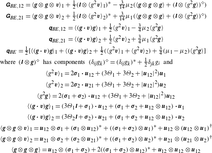
Third-order tensors
 $\unicode[STIX]{x1D642}_{BE}$
and contracted first-order tensor
 $\unicode[STIX]{x1D666}_{BE}$
appearing in the energy conservation equations. In these expressions, the vectors
 $\boldsymbol{u}_{1}$
,
 $\boldsymbol{u}_{2}$
,
 $\boldsymbol{u}_{12}$
and
 $\boldsymbol{u}_{21}=-\boldsymbol{u}_{12}$
, and the velocity covariance tensors
 $\unicode[STIX]{x1D748}_{1}$
and
 $\unicode[STIX]{x1D748}_{2}$
appear. For isotropic systems,
 $\unicode[STIX]{x1D748}_{\unicode[STIX]{x1D6FC}}=\unicode[STIX]{x1D6E9}_{\unicode[STIX]{x1D6FC}}\unicode[STIX]{x1D644}$
and the formulae simplify considerably. The third-order tensors have the symmetry property
 $\unicode[STIX]{x1D60E}_{ijk}=\unicode[STIX]{x1D60E}_{ikj}$
. Using these definitions and
 $\unicode[STIX]{x1D707}_{1}+\unicode[STIX]{x1D707}_{2}=2$
, it is straightforward to prove that
 $\unicode[STIX]{x1D666}_{BE,12}=\unicode[STIX]{x1D666}_{BE,21}$
. Thus, we define
 $\unicode[STIX]{x1D666}_{BE}:=\frac{1}{2}(\unicode[STIX]{x1D666}_{BE,12}+\unicode[STIX]{x1D666}_{BE,21})$
. As a corollary,
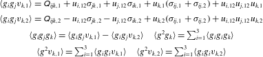
 $\unicode[STIX]{x1D642}_{BE,12}-\unicode[STIX]{x1D642}_{BE,21}=\frac{1}{14}[8\langle \boldsymbol{g}\otimes \boldsymbol{g}\otimes \boldsymbol{g}\rangle +(\unicode[STIX]{x1D644}\otimes \langle g^{2}\boldsymbol{g}\rangle )^{\ast }-3\langle g^{2}\boldsymbol{g}\rangle \otimes \unicode[STIX]{x1D644}]$
and contraction of the difference is null. Finally, note that
 $\langle g^{2}\boldsymbol{g}\rangle +|\boldsymbol{u}_{12}|^{2}\boldsymbol{u}_{21}$
is proportional to
 $\unicode[STIX]{x1D64B}_{BE}\boldsymbol{\cdot }\boldsymbol{u}_{12}$
, which can be used to re-express
 $\unicode[STIX]{x1D666}_{BE}$
with terms involving
 $\unicode[STIX]{x1D64B}_{BE}$
.

3.4 Total energy balances
Balances for the total energy in each phase,
 $\unicode[STIX]{x1D71A}_{\unicode[STIX]{x1D6FC}}E_{\unicode[STIX]{x1D6FC}}:=\unicode[STIX]{x1D71A}_{\unicode[STIX]{x1D6FC}}\text{tr}(\unicode[STIX]{x1D640}_{\unicode[STIX]{x1D6FC}})$
, can be found by taking the trace of (3.11). This leads to
 $$\begin{eqnarray}\left.\begin{array}{@{}c@{}}\unicode[STIX]{x2202}_{t}\unicode[STIX]{x1D71A}_{1}E_{1}+\unicode[STIX]{x2202}_{\boldsymbol{x}}\boldsymbol{\cdot }(\unicode[STIX]{x1D71A}_{1}\boldsymbol{u}_{1}E_{1}+\unicode[STIX]{x1D71A}_{1}\unicode[STIX]{x1D748}_{1}\boldsymbol{\cdot }\boldsymbol{u}_{1}+\unicode[STIX]{x1D64B}_{1}\boldsymbol{\cdot }\boldsymbol{u}_{1}+\unicode[STIX]{x1D666}_{12})=C_{E}+D_{E},\\ ~\unicode[STIX]{x2202}_{t}\unicode[STIX]{x1D71A}_{2}E_{2}+\unicode[STIX]{x2202}_{\boldsymbol{x}}\boldsymbol{\cdot }(\unicode[STIX]{x1D71A}_{2}\boldsymbol{u}_{2}E_{2}+\unicode[STIX]{x1D71A}_{2}\unicode[STIX]{x1D748}_{2}\boldsymbol{\cdot }\boldsymbol{u}_{2}+\unicode[STIX]{x1D64B}_{2}\boldsymbol{\cdot }\boldsymbol{u}_{2}+\unicode[STIX]{x1D666}_{21})=-C_{E}-D_{E},\end{array}\right\}\end{eqnarray}$$
where the drag exchange term is given by (as done for
 $\unicode[STIX]{x1D666}_{BE}$
in table 1, we use the symmetric form for
 $D_{E}$
)
 $$\begin{eqnarray}D_{E}:={\textstyle \frac{1}{2}}(\text{tr}(\boldsymbol{D}_{0,12})-\text{tr}(\boldsymbol{D}_{0,21}))={\textstyle \frac{3}{2}}K[\unicode[STIX]{x1D707}_{2}\unicode[STIX]{x1D6E9}_{2}-\unicode[STIX]{x1D707}_{1}\unicode[STIX]{x1D6E9}_{1}-{\textstyle \frac{1}{3}}(\unicode[STIX]{x1D707}_{2}\boldsymbol{u}_{2}+\unicode[STIX]{x1D707}_{1}\boldsymbol{u}_{1})\boldsymbol{\cdot }\boldsymbol{u}_{12}],\end{eqnarray}$$
and the energy fluxes by
 $$\begin{eqnarray}\unicode[STIX]{x1D666}_{12}:={\textstyle \frac{1}{5}}{\mathcal{V}}_{12}\unicode[STIX]{x1D707}_{2}\unicode[STIX]{x1D71A}_{1}\unicode[STIX]{x1D711}_{2}g_{12}\unicode[STIX]{x1D666}_{BE},\quad \unicode[STIX]{x1D666}_{21}:={\textstyle \frac{1}{5}}{\mathcal{V}}_{12}\unicode[STIX]{x1D707}_{1}\unicode[STIX]{x1D71A}_{2}\unicode[STIX]{x1D711}_{1}g_{12}\unicode[STIX]{x1D666}_{BE}.\end{eqnarray}$$
The BE collisional correction to the energy flux
 $\unicode[STIX]{x1D666}_{BE}$
has components
 $\unicode[STIX]{x1D632}_{BE,i}:=\sum _{j}\unicode[STIX]{x1D60E}_{BE,ijj}$
(see table 1). The total-energy-exchange term is given by
 $$\begin{eqnarray}C_{E}:=\text{tr}(\boldsymbol{D}_{1,12})={\textstyle \frac{1}{5}}\unicode[STIX]{x1D707}_{2}\unicode[STIX]{x1D711}_{2}(\unicode[STIX]{x2202}_{\boldsymbol{x}}-\unicode[STIX]{x2202}_{\boldsymbol{x}}^{(2)})\boldsymbol{\cdot }\unicode[STIX]{x1D71A}_{1}h_{1}\unicode[STIX]{x1D666}_{BE}-{\textstyle \frac{1}{5}}\unicode[STIX]{x1D707}_{1}\unicode[STIX]{x1D711}_{1}(\unicode[STIX]{x2202}_{\boldsymbol{x}}-\unicode[STIX]{x2202}_{\boldsymbol{x}}^{(1)})\boldsymbol{\cdot }\unicode[STIX]{x1D71A}_{2}h_{2}\unicode[STIX]{x1D666}_{BE}.\end{eqnarray}$$
Thus, we can observe that the system total energy
 $\unicode[STIX]{x1D71A}E:=\unicode[STIX]{x1D71A}_{1}E_{1}+\unicode[STIX]{x1D71A}_{2}E_{2}$
is a conserved quantity. It is worth noting the important contribution of the relative velocity
 $\boldsymbol{u}_{12}$
in the production and exchange of energy between the two phases. At equilibrium, the mass ratios
 $\unicode[STIX]{x1D707}_{\unicode[STIX]{x1D6FC}}$
determine the energy distribution between the two phases.
3.5 Covariance tensors and fluctuating energy
Balance equations for the covariance tensors can be derived by subtracting off the contributions from the mean kinetic energy tensor
 $\unicode[STIX]{x1D71A}_{\unicode[STIX]{x1D6FC}}\unicode[STIX]{x1D646}_{\unicode[STIX]{x1D6FC}}:=\frac{1}{2}\unicode[STIX]{x1D71A}_{\unicode[STIX]{x1D6FC}}\boldsymbol{u}_{\unicode[STIX]{x1D6FC}}\otimes \boldsymbol{u}_{\unicode[STIX]{x1D6FC}}$
in (3.11). First, starting from the mean momentum balances, we derive balances for the mean kinetic energy tensors
 $$\begin{eqnarray}\left.\begin{array}{@{}l@{}}\unicode[STIX]{x2202}_{t}\unicode[STIX]{x1D71A}_{1}\unicode[STIX]{x1D646}_{1}+\unicode[STIX]{x2202}_{\boldsymbol{x}}\boldsymbol{\cdot }\unicode[STIX]{x1D71A}_{1}\boldsymbol{u}_{1}\otimes \unicode[STIX]{x1D646}_{1}+(\boldsymbol{u}_{1}\otimes \unicode[STIX]{x2202}_{\boldsymbol{x}}\boldsymbol{\cdot }(\unicode[STIX]{x1D71A}_{1}\unicode[STIX]{x1D748}_{1}+\unicode[STIX]{x1D64B}_{1}+\unicode[STIX]{x1D64B}_{12}))^{\dagger }~\\ \quad =(\boldsymbol{u}_{1}\otimes \boldsymbol{C}-K\boldsymbol{u}_{1}\otimes \boldsymbol{u}_{12})^{\dagger },~\\ \unicode[STIX]{x2202}_{t}\unicode[STIX]{x1D71A}_{p}\unicode[STIX]{x1D646}_{2}+\unicode[STIX]{x2202}_{\boldsymbol{x}}\boldsymbol{\cdot }\unicode[STIX]{x1D71A}_{2}\boldsymbol{u}_{2}\otimes \unicode[STIX]{x1D646}_{2}+(\boldsymbol{u}_{2}\otimes \unicode[STIX]{x2202}_{\boldsymbol{x}}\boldsymbol{\cdot }(\unicode[STIX]{x1D71A}_{2}\unicode[STIX]{x1D748}_{2}+\unicode[STIX]{x1D64B}_{2}+\unicode[STIX]{x1D64B}_{21}))^{\dagger }\\ ~\quad =-(\boldsymbol{u}_{2}\otimes \boldsymbol{C}-K\boldsymbol{u}_{2}\otimes \boldsymbol{u}_{12})^{\dagger }.\end{array}\right\}\end{eqnarray}$$
We then subtract these expressions from the total energy tensor balances to find
 $$\begin{eqnarray}\left.\begin{array}{@{}l@{}}{\textstyle \frac{1}{2}}\unicode[STIX]{x2202}_{t}\unicode[STIX]{x1D71A}_{1}\unicode[STIX]{x1D748}_{1}+{\textstyle \frac{1}{2}}\unicode[STIX]{x2202}_{\boldsymbol{x}}\boldsymbol{\cdot }\unicode[STIX]{x1D71A}_{1}\boldsymbol{u}_{1}\otimes \unicode[STIX]{x1D748}_{1}+((\unicode[STIX]{x1D71A}_{1}\unicode[STIX]{x1D748}_{1}+\unicode[STIX]{x1D64B}_{1})\boldsymbol{\cdot }\unicode[STIX]{x2202}_{\boldsymbol{x}}\boldsymbol{u}_{1})^{\dagger }+\unicode[STIX]{x2202}_{\boldsymbol{ x}}\boldsymbol{\cdot }\unicode[STIX]{x1D642}_{12}-(\boldsymbol{u}_{1}\otimes \unicode[STIX]{x2202}_{\boldsymbol{x}}\boldsymbol{\cdot }\unicode[STIX]{x1D64B}_{12})^{\dagger }\\ ~\quad =\boldsymbol{D}_{1}+\boldsymbol{D}_{0,12}+K(\boldsymbol{u}_{1}\otimes \boldsymbol{u}_{12})^{\dagger }+\boldsymbol{D}_{1,12}-(\boldsymbol{u}_{1}\otimes \boldsymbol{C})^{\dagger },\\ ~{\textstyle \frac{1}{2}}\unicode[STIX]{x2202}_{t}\unicode[STIX]{x1D71A}_{2}\unicode[STIX]{x1D748}_{2}+{\textstyle \frac{1}{2}}\unicode[STIX]{x2202}_{\boldsymbol{x}}\boldsymbol{\cdot }\unicode[STIX]{x1D71A}_{2}\boldsymbol{u}_{2}\otimes \unicode[STIX]{x1D748}_{2}+((\unicode[STIX]{x1D71A}_{2}\unicode[STIX]{x1D748}_{2}+\unicode[STIX]{x1D64B}_{2})\boldsymbol{\cdot }\unicode[STIX]{x2202}_{\boldsymbol{x}}\boldsymbol{u}_{2})^{\dagger }+\unicode[STIX]{x2202}_{\boldsymbol{ x}}\boldsymbol{\cdot }\unicode[STIX]{x1D642}_{21}-(\boldsymbol{u}_{2}\otimes \unicode[STIX]{x2202}_{\boldsymbol{x}}\boldsymbol{\cdot }\unicode[STIX]{x1D64B}_{21})^{\dagger }\\ ~\quad =\boldsymbol{D}_{2}+\boldsymbol{D}_{0,21}-K(\boldsymbol{u}_{2}\otimes \boldsymbol{u}_{12})^{\dagger }+\boldsymbol{D}_{1,21}+(\boldsymbol{u}_{2}\otimes \boldsymbol{C})^{\dagger }.\end{array}\right\}\end{eqnarray}$$
The velocity covariance tensors will be non-zero if there is a non-zero mean-slip velocity. Also, in general, they will be anisotropic due to the anisotropy of their source terms.
The traces of the velocity covariance tensors in (3.21) lead to the fluctuating energy balance equations
 $$\begin{eqnarray}\left.\begin{array}{@{}l@{}}\frac{3}{2}\unicode[STIX]{x2202}_{t}\unicode[STIX]{x1D71A}_{1}\unicode[STIX]{x1D6E9}_{1}+\frac{3}{2}\unicode[STIX]{x2202}_{\boldsymbol{x}}\boldsymbol{\cdot }\unicode[STIX]{x1D71A}_{1}\boldsymbol{u}_{1}\unicode[STIX]{x1D6E9}_{1}+(\unicode[STIX]{x1D71A}_{1}\unicode[STIX]{x1D748}_{1}+\unicode[STIX]{x1D64B}_{1})\boldsymbol{ : }\unicode[STIX]{x2202}_{\boldsymbol{x}}\boldsymbol{u}_{1}+\unicode[STIX]{x2202}_{\boldsymbol{x}}\boldsymbol{\cdot }\unicode[STIX]{x1D666}_{12}-\boldsymbol{u}_{1}\boldsymbol{\cdot }(\unicode[STIX]{x2202}_{\boldsymbol{x}}\boldsymbol{\cdot }\unicode[STIX]{x1D64B}_{12})\\[3.0pt] \quad =D_{E}+K\boldsymbol{u}_{1}\boldsymbol{\cdot }\boldsymbol{u}_{12}+C_{E}-\boldsymbol{u}_{1}\boldsymbol{\cdot }\boldsymbol{C},\\[3.0pt] \frac{3}{2}\unicode[STIX]{x2202}_{t}\unicode[STIX]{x1D71A}_{2}\unicode[STIX]{x1D6E9}_{2}+\frac{3}{2}\unicode[STIX]{x2202}_{\boldsymbol{x}}\boldsymbol{\cdot }\unicode[STIX]{x1D71A}_{2}\boldsymbol{u}_{2}\unicode[STIX]{x1D6E9}_{2}+(\unicode[STIX]{x1D71A}_{2}\unicode[STIX]{x1D748}_{2}+\unicode[STIX]{x1D64B}_{2})\boldsymbol{ : }\unicode[STIX]{x2202}_{\boldsymbol{x}}\boldsymbol{u}_{2}+\unicode[STIX]{x2202}_{\boldsymbol{x}}\boldsymbol{\cdot }\unicode[STIX]{x1D666}_{21}-\boldsymbol{u}_{2}\boldsymbol{\cdot }(\unicode[STIX]{x2202}_{\boldsymbol{x}}\boldsymbol{\cdot }\unicode[STIX]{x1D64B}_{21})\\[3.0pt] \quad =-D_{E}-K\boldsymbol{u}_{2}\boldsymbol{\cdot }\boldsymbol{u}_{12}-C_{E}+\boldsymbol{u}_{2}\boldsymbol{\cdot }\boldsymbol{C},\end{array}\right\}\end{eqnarray}$$
which govern the phase temperatures. The terms on the left-hand sides involving the phase pressure tensors correspond to compression heating. The other terms on the right-hand side are production/redistribution of fluctuating energy between phases. The sum of the two balances in (3.22) is the total fluctuating energy. For the latter, we can observe that there is a source term
 $K|\boldsymbol{u}_{12}|^{2}$
due to the transfer of mean kinetic energy to fluctuations when the phases have a mean-slip velocity. On the other hand,
 $\boldsymbol{u}_{21}\boldsymbol{\cdot }\boldsymbol{C}$
can function as a source or sink of fluctuating energy depending on the signs of the gradients appearing in
 $\boldsymbol{C}$
. These observations imply that even in the absence of mean gradients, the phase temperatures will be non-zero if the phases are initially in relative mean motion. Finally, using the momentum balances in (3.4) and (3.22), it is possible to derive the balance equation for the ‘mixture’ temperature
 $\unicode[STIX]{x1D6E9}$
.
3.6 Equilibrium state
The equilibrium state for a homogeneous, binary system is
 $\boldsymbol{u}_{1}=\boldsymbol{u}_{2}$
,
 $\unicode[STIX]{x1D707}_{1}\unicode[STIX]{x1D6E9}_{1}=\unicode[STIX]{x1D707}_{2}\unicode[STIX]{x1D6E9}_{2}$
and
 $\unicode[STIX]{x1D748}_{\unicode[STIX]{x1D6FC}}=\unicode[STIX]{x1D6E9}_{\unicode[STIX]{x1D6FC}}\unicode[STIX]{x1D644}$
(see, e.g. Kolodner Reference Kolodner1957; Grad Reference Grad and Devienne1960; Morse Reference Morse1963; Goldman & Sirovich Reference Goldman and Sirovich1967), and the densities, velocities and temperatures are spatially uniform. The functions
 $h_{1}$
and
 $h_{2}$
introduced in (2.6) are chosen such that the isotropic flux pressure, i.e. for type-1 particles
 $$\begin{eqnarray}\unicode[STIX]{x1D71A}_{1}\unicode[STIX]{x1D748}_{1}+\unicode[STIX]{x1D64B}_{1}+\unicode[STIX]{x1D64B}_{12}=\unicode[STIX]{x1D71A}_{1}\unicode[STIX]{x1D6E9}_{1}(1+{\mathcal{V}}_{11}\unicode[STIX]{x1D711}_{1}g_{0}+{\mathcal{V}}_{12}\unicode[STIX]{x1D711}_{2}g_{12})\unicode[STIX]{x1D644}=p_{1}\unicode[STIX]{x1D644},\end{eqnarray}$$
and the buoyancy pressure, defined to be the non-zero term in
 $\boldsymbol{C}$
at equilibrium, i.e. for type-1 particles (the other terms in
 $\boldsymbol{C}$
depend on gradients in density and velocity and correspond to forces other than the buoyancy force)
 $$\begin{eqnarray}{\textstyle \frac{1}{5}}\unicode[STIX]{x1D707}_{2}\unicode[STIX]{x1D71A}_{1}h_{1}\unicode[STIX]{x1D64B}_{BE}|_{eq}=\unicode[STIX]{x1D71A}_{1}\unicode[STIX]{x1D6E9}_{1}h_{1}\unicode[STIX]{x1D644}=p_{1}\unicode[STIX]{x1D644},\end{eqnarray}$$
are identical for each particle type. In equilibrium, the phase pressures are isotropic and the momentum balances reduce to
 $$\begin{eqnarray}\unicode[STIX]{x2202}_{\boldsymbol{x}}p_{1}=\unicode[STIX]{x1D711}_{2}\unicode[STIX]{x2202}_{\boldsymbol{x}}p_{1}-\unicode[STIX]{x1D711}_{1}\unicode[STIX]{x2202}_{\boldsymbol{x}}p_{2},\quad \unicode[STIX]{x2202}_{\boldsymbol{x}}p_{2}=\unicode[STIX]{x1D711}_{1}\unicode[STIX]{x2202}_{\boldsymbol{x}}p_{2}-\unicode[STIX]{x1D711}_{2}\unicode[STIX]{x2202}_{\boldsymbol{x}}p_{1}.\end{eqnarray}$$
Thus,
 $\unicode[STIX]{x2202}_{\boldsymbol{x}}(p_{1}+p_{2})=\mathbf{0}$
, i.e. the mixture pressure is uniform, and hence
 $\unicode[STIX]{x2202}_{\boldsymbol{x}}p_{1}=-\unicode[STIX]{x2202}_{\boldsymbol{x}}p_{2}$
. It then follows that in order for the above momentum balances to hold,
 $\unicode[STIX]{x2202}_{\boldsymbol{x}}p_{\unicode[STIX]{x1D6FC}}=\mathbf{0}$
at equilibrium, i.e. the phase pressures must be uniform.
If the mean momentum is initially null,
 $\unicode[STIX]{x1D71A}_{1}\boldsymbol{u}_{1}+\unicode[STIX]{x1D71A}_{2}\boldsymbol{u}_{2}=\mathbf{0}$
but
 $\boldsymbol{u}_{1}\neq \boldsymbol{u}_{2}$
, then at equilibrium
 $\boldsymbol{u}_{1}=\boldsymbol{u}_{2}=\mathbf{0}$
and the mean kinetic energy will be transferred to
 $\unicode[STIX]{x1D6E9}_{\unicode[STIX]{x1D6FC}}$
through collisions. Thus, in the limit where
 $\unicode[STIX]{x1D707}_{1}\ll \unicode[STIX]{x1D707}_{2}$
, the phase temperatures will be very different at equilibrium with
 $\unicode[STIX]{x1D6E9}_{2}\ll \unicode[STIX]{x1D6E9}_{1}$
. (For systems in motion,
 $\unicode[STIX]{x1D6E9}_{2}$
has a source term due to phase compression and, hence, can be much larger than its equilibrium value. For fluid–particle systems in § 4, the equilibrium value of
 $\unicode[STIX]{x1D6E9}_{2}$
is essentially zero.) As the particles are assumed to have no internal degrees of freedom, their internal energies are null. In the absence of external forces (e.g. gravity), the mean momentum and total energy of the system are conserved. As first described by Grad (Reference Grad and Devienne1960), the rates of relaxation to equilibrium for the mean velocities and granular temperatures can be very different for components with disparate masses. For example, under certain conditions (e.g. plasmas) the mean velocities will rapidly equilibrate so that only the two temperatures differ (i.e. the so-called two-temperature model (Sirovich Reference Sirovich1962)). Hereinafter, we will focus on cases for which a two-fluid description is required, i.e. the heavy component is a trace component with very small molar concentration as first described in Hamel (Reference Hamel1966).
4 The fluid–particle limit
The balances derived in the previous section hold for any binary, non-dissipative, hard-sphere mixture. We now want to consider the case where
 $d_{1}\ll d_{2}$
and
 $\unicode[STIX]{x1D707}_{1}\ll \unicode[STIX]{x1D707}_{2}$
, which corresponds to phase 1 being a molecular hard-sphere fluid and phase 2 composed of macroscopic particles. (See Zhang et al. (Reference Zhang, Ma and Rauenzahn2006) for a discussion of this limit for arbitrary binary interaction forces.) Furthermore, we will assume that the VDFs are Maxwellian, i.e.
 $\unicode[STIX]{x1D748}_{\unicode[STIX]{x1D6FC}}=\unicode[STIX]{x1D6E9}_{\unicode[STIX]{x1D6FC}}\unicode[STIX]{x1D644}$
. This assumption decreases significantly the number of variables in the two-fluid model (Levermore & Morokoff Reference Levermore and Morokoff1996). However, with finite-size (type-2) particles, it is more accurate to solve for
 $\unicode[STIX]{x1D748}_{2}$
using the anisotropic Gaussian model (Levermore & Morokoff Reference Levermore and Morokoff1996; Vié et al.
Reference Vié, Doisneau and Massot2015; Kong et al.
Reference Kong, Fox, Feng, Capecelatro, Patel and Desjardins2017; Patel et al.
Reference Patel, Desjardins, Kong, Capecelatro and Fox2017). By definition, the volume fraction occupied by type-
 $\unicode[STIX]{x1D6FC}$
particles is
 $\unicode[STIX]{x1D711}_{\unicode[STIX]{x1D6FC}}=\unicode[STIX]{x1D71A}_{\unicode[STIX]{x1D6FC}}/\unicode[STIX]{x1D70C}_{\unicode[STIX]{x1D6FC}}$
, and the total occupied volume fraction is
 $\unicode[STIX]{x1D711}=\unicode[STIX]{x1D711}_{1}+\unicode[STIX]{x1D711}_{2}$
. Thus, when
 $\unicode[STIX]{x1D711}_{1}$
is negligibly small relative to
 $\unicode[STIX]{x1D711}_{2}$
, the fluid phase will be a perfect gas and terms involving
 $\unicode[STIX]{x1D71A}_{1}\unicode[STIX]{x1D711}_{1}$
can be dropped. Otherwise, the fluid phase will be a non-ideal gas (i.e. a hard-sphere fluid). In terms of the mole fractions, that of phase 2 is negligible because the number of type-1 particles is allowed to go to infinity as
 $d_{1}$
goes to zero such that
 $\unicode[STIX]{x1D711}_{1}$
remains constant. Thus, type-2 particles are a trace component in the sense of Hamel (Reference Hamel1966). Finally, the Maxwellian assumption for the fluid phase implies that the fluid is inviscid and hence governed by the Euler equation in the absence of particles.
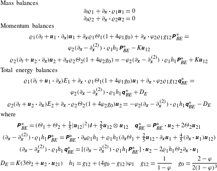
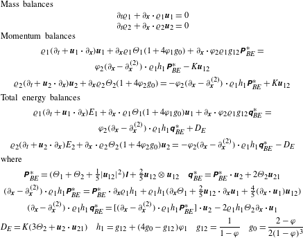
Fluid–particle model for a binary, hard-sphere mixture with independent variables (
 $\unicode[STIX]{x1D71A}_{\unicode[STIX]{x1D6FC}},\boldsymbol{u}_{\unicode[STIX]{x1D6FC}},E_{\unicode[STIX]{x1D6FC}}$
). The operator
 $(\unicode[STIX]{x2202}_{\boldsymbol{x}}-\unicode[STIX]{x2202}_{\boldsymbol{x}}^{(2)})$
produces gradients of the variables (
 $\unicode[STIX]{x1D71A}_{1},\boldsymbol{u}_{1},E_{1},\unicode[STIX]{x1D71A}_{2}$
), i.e.
 $(\unicode[STIX]{x2202}_{\boldsymbol{x}}-\unicode[STIX]{x2202}_{\boldsymbol{x}}^{(2)})\boldsymbol{\cdot }\boldsymbol{u}_{2}=0$
and
 $(\unicode[STIX]{x2202}_{\boldsymbol{x}}-\unicode[STIX]{x2202}_{\boldsymbol{x}}^{(2)})E_{2}=0$
. In this two-fluid model, the material densities
 $\unicode[STIX]{x1D70C}_{1}$
and
 $\unicode[STIX]{x1D70C}_{2}$
are constant and the volume fractions
 $\unicode[STIX]{x1D711}_{\unicode[STIX]{x1D6FC}}$
are found from
 $\unicode[STIX]{x1D71A}_{\unicode[STIX]{x1D6FC}}=\unicode[STIX]{x1D70C}_{\unicode[STIX]{x1D6FC}}\unicode[STIX]{x1D711}_{\unicode[STIX]{x1D6FC}}$
. The other variables appearing in the model are
 $\unicode[STIX]{x1D711}=\unicode[STIX]{x1D711}_{1}+\unicode[STIX]{x1D711}_{2}$
,
 $\boldsymbol{u}_{12}=-\boldsymbol{u}_{21}=\boldsymbol{u}_{1}-\boldsymbol{u}_{2}$
, and
 $\unicode[STIX]{x1D6E9}_{\unicode[STIX]{x1D6FC}}=\frac{2}{3}(E_{\unicode[STIX]{x1D6FC}}-\frac{1}{2}|\boldsymbol{u}_{\unicode[STIX]{x1D6FC}}|^{2})$
. Note that
 $\unicode[STIX]{x1D64B}_{BE}^{\ast }:=\frac{2}{5}\unicode[STIX]{x1D64B}_{BE}$
and
 $\unicode[STIX]{x1D666}_{BE}^{\ast }:=\frac{2}{5}\unicode[STIX]{x1D666}_{BE}$
. For a perfect gas,
 $\unicode[STIX]{x1D71A}_{1}=\unicode[STIX]{x1D70C}_{1}\unicode[STIX]{x1D711}_{1}=\unicode[STIX]{x1D70C}_{f}(1-\unicode[STIX]{x1D711}_{2})$
is finite in the limit
 $\unicode[STIX]{x1D711}_{1}\rightarrow 0$
with fluid density
 $\unicode[STIX]{x1D70C}_{f}$
and void fraction
 $\unicode[STIX]{x1D6FC}_{f}:=1-\unicode[STIX]{x1D711}_{2}$
, in which case
 $p_{f}:=\unicode[STIX]{x1D70C}_{f}\unicode[STIX]{x1D6E9}_{1}$
is the fluid pressure.
In the fluid limit where
 $d_{1}\ll d_{2}$
, the parameters appearing in the balance equations can be approximated as follows:
 $$\begin{eqnarray}\left.\begin{array}{@{}c@{}}{\mathcal{V}}_{12}=1,~g_{12}={\displaystyle \frac{1}{1-\unicode[STIX]{x1D711}}},\unicode[STIX]{x1D707}_{1}=0,\unicode[STIX]{x1D707}_{2}=2,\quad K={\displaystyle \frac{6\unicode[STIX]{x1D71A}_{1}\unicode[STIX]{x1D711}_{2}\sqrt{\unicode[STIX]{x1D6E9}/2}}{d_{2}(1-\unicode[STIX]{x1D711})}},\\[5.0pt] h_{1}={\displaystyle \frac{1-\unicode[STIX]{x1D711}_{1}}{1-\unicode[STIX]{x1D711}}}+4\unicode[STIX]{x1D711}_{1}g_{0},\quad h_{2}={\displaystyle \frac{1-\unicode[STIX]{x1D711}_{2}}{1-\unicode[STIX]{x1D711}}}+4\unicode[STIX]{x1D711}_{2}g_{0}.\end{array}\right\}\end{eqnarray}$$
The parameters,
 $\unicode[STIX]{x1D70C}_{1}$
,
 $\unicode[STIX]{x1D70C}_{2}$
and
 $d_{2}$
are constants. The fluid–particle model solves for state variables:
 $(\unicode[STIX]{x1D71A}_{1},\unicode[STIX]{x1D71A}_{2},\boldsymbol{u}_{1},\boldsymbol{u}_{2},E_{1},E_{2})$
. For completeness, we provide the complete three-dimensional (3-D) two-fluid model written in these variables in table 2. In § 5, we investigate the hyperbolicity of the one-dimensional (1-D) model for various sets of parameters, including for a perfect gas. For clarity, in the remainder of this section, we will consider only the case where the fluid is a perfect gas. This corresponds to neglecting
 $\unicode[STIX]{x1D711}_{1}$
and replacing
 $\unicode[STIX]{x1D71A}_{1}=\unicode[STIX]{x1D70C}_{f}\unicode[STIX]{x1D6FC}_{f}$
and
 $\unicode[STIX]{x1D71A}_{2}=\unicode[STIX]{x1D70C}_{p}\unicode[STIX]{x1D6FC}_{p}$
. By definition,
 $\unicode[STIX]{x1D6FC}_{f}:=1-\unicode[STIX]{x1D6FC}_{p}$
and
 $\unicode[STIX]{x1D6FC}_{p}:=\unicode[STIX]{x1D711}_{2}$
, and
 $\unicode[STIX]{x1D6FC}_{f}g_{12}=\unicode[STIX]{x1D6FC}_{f}h_{1}=1$
. The fluid pressure is then defined as
 $p_{f}=\unicode[STIX]{x1D70C}_{f}\unicode[STIX]{x1D6E9}_{f}$
and
 $p_{p}=\unicode[STIX]{x1D70C}_{p}\unicode[STIX]{x1D6FC}_{p}\unicode[STIX]{x1D6E9}_{p}(1+4\unicode[STIX]{x1D6FC}_{p}g_{0})$
is the granular pressure. In general, the subscript
 $\text{}_{f}$
denotes type-1 particles and
 $\text{}_{p}$
denotes type-2 particles.
Compressible gas–particle two-fluid model for elastic hard-sphere particles in an ideal gas with
 $\unicode[STIX]{x1D70C}_{f}\ll \unicode[STIX]{x1D70C}_{p}$
. The particle material density
 $\unicode[STIX]{x1D70C}_{p}$
is constant and the specific heat ratios are
 $\unicode[STIX]{x1D6FE}_{f}$
and
 $\unicode[STIX]{x1D6FE}_{p}=5/3$
. The stress tensor
 $\unicode[STIX]{x1D64D}$
, energy flux
 $\boldsymbol{r}$
, momentum exchange
 $\unicode[STIX]{x1D641}_{pf}$
and energy exchange
 $D_{pf}$
arise due to the finite-size particles. For constant fluid density, only the term involving
 $\unicode[STIX]{x1D64E}$
is significant in
 $\unicode[STIX]{x1D641}_{pf}$
, providing a model for the lift force.
 $K$
is the drag coefficient that depends on the particle Reynolds number, Mach number and volume fraction. The second term in
 $\unicode[STIX]{x1D641}_{pf}$
, resulting from fluid compressibility, can be combined with the drag force. The first term in
 $\unicode[STIX]{x1D641}_{pf}$
has the form of a dispersion force, but resulting here from fluid-density gradients. A constant body force
 $\boldsymbol{g}$
is included for completeness (see appendix B).

For convenience, the model equations for the ideal-gas case are provided in table 3 and have the form employed in ‘classical’ two-fluid models for compressible gas–particle flows, albeit with additional terms due to fluid compressibility and fluid-velocity gradients arising from the BE tensors for finite-size particles. Note, as expected, that for
 $\unicode[STIX]{x1D6FC}_{p}=0$
the fluid phase reduces to the Euler equation of gas dynamics. The BE tensors depend on
 $$\begin{eqnarray}(\unicode[STIX]{x2202}_{\boldsymbol{x}}-\unicode[STIX]{x2202}_{\boldsymbol{x}}^{(2)})\boldsymbol{\cdot }\unicode[STIX]{x1D70C}_{f}\unicode[STIX]{x1D64D}=\unicode[STIX]{x1D64D}\boldsymbol{\cdot }\unicode[STIX]{x2202}_{\boldsymbol{x}}\unicode[STIX]{x1D70C}_{f}+\unicode[STIX]{x1D70C}_{f}\unicode[STIX]{x2202}_{\boldsymbol{x}}^{(1)}\boldsymbol{\cdot }\unicode[STIX]{x1D64D},\end{eqnarray}$$
where
 $\unicode[STIX]{x2202}_{\boldsymbol{x}}^{(1)}\boldsymbol{\cdot }\unicode[STIX]{x1D64D}=\frac{4}{5}\boldsymbol{u}_{fp}\boldsymbol{\cdot }\unicode[STIX]{x1D71E}+\frac{2}{5}\text{tr}(\unicode[STIX]{x1D71E})\boldsymbol{u}_{fp}$
and
 $\unicode[STIX]{x1D71E}$
is the rate-of-deformation tensor for the fluid phase. In (4.2),
 $\unicode[STIX]{x2202}_{\boldsymbol{x}}^{(1)}\boldsymbol{\cdot }\unicode[STIX]{x1D64D}$
can be further decomposed into an isotropic and a traceless component, yielding the second and third terms, respectively, in the exchange force
 $$\begin{eqnarray}\unicode[STIX]{x1D641}_{pf}=\unicode[STIX]{x1D6FC}_{p}\unicode[STIX]{x1D64D}\boldsymbol{\cdot }\unicode[STIX]{x2202}_{\boldsymbol{x}}\unicode[STIX]{x1D70C}_{f}+{\textstyle \frac{2}{3}}\unicode[STIX]{x1D6FC}_{p}\unicode[STIX]{x1D70C}_{f}(\unicode[STIX]{x2202}_{\boldsymbol{x}}\boldsymbol{\cdot }\boldsymbol{u}_{f})\boldsymbol{u}_{fp}+{\textstyle \frac{4}{5}}\unicode[STIX]{x1D6FC}_{p}\unicode[STIX]{x1D70C}_{f}\unicode[STIX]{x1D64E}\boldsymbol{\cdot }\boldsymbol{u}_{fp}.\end{eqnarray}$$
Analogous manipulations on
 $\unicode[STIX]{x1D70C}_{f}\boldsymbol{r}$
lead to
 $D_{pf}$
. It is important to notice that the buoyancy force due to
 $p_{f}=\unicode[STIX]{x1D70C}_{f}\unicode[STIX]{x1D6E9}_{f}$
is not included among the exchange forces in (4.3), as it appears separately on the left-hand side of the momentum balances. When the fluid density is constant, the first two terms on the right-hand side of (4.3) will be null or negligible. (Aside from
 $g_{0}$
in
 $p_{p}$
, the kinetic-theory model does not account for nonlinear terms in
 $\unicode[STIX]{x1D6FC}_{p}$
. Thus, when
 $\unicode[STIX]{x1D70C}_{f}$
is constant,
 $\unicode[STIX]{x2202}_{\boldsymbol{x}}\boldsymbol{\cdot }\boldsymbol{u}_{f}=0$
up to first order in
 $\unicode[STIX]{x1D6FC}_{p}$
. For a perfect gas, non-zero
 $\unicode[STIX]{x2202}_{\boldsymbol{x}}\unicode[STIX]{x1D70C}_{f}$
at constant
 $p_{f}=\unicode[STIX]{x1D70C}_{f}\unicode[STIX]{x1D6E9}_{f}$
implies that a fluid temperature gradient exists.) The third term involving the fluid strain-rate tensor
 $\unicode[STIX]{x1D64E}$
can be further decomposed into a force component in the direction
 $\boldsymbol{u}_{fp}$
and a tangential force. The former can be combined with the drag force, while the latter represents a lift force. Furthermore, from the point of view of hyperbolicity, the terms involving
 $\unicode[STIX]{x1D6E9}_{p}$
in
 $\unicode[STIX]{x1D64D}$
and
 $\boldsymbol{r}$
can be dropped when
 $\unicode[STIX]{x1D6E9}_{p}$
, scaled by the speed of sound in the fluid, is small. (The eigenvalues of the particle phase depend on
 $\unicode[STIX]{x1D6E9}_{p}$
through
 $p_{p}$
.) Indeed, dropping the contribution in
 $\boldsymbol{r}$
significantly simplifies the characteristic equation discussed in § 5.3 and slightly increases the region of hyperbolicity. In practice, all of the terms (including those in
 $\unicode[STIX]{x1D64D}$
) in the direction
 $\boldsymbol{u}_{fp}$
can be combined with the drag force. Then, as is done for the drag coefficient
 $K$
, the lift-force definition can be modified to account for viscous flow physics without changing the hyperbolicity of the two-fluid model. Except perhaps across a shock wave, the forces in (4.3) arising due to fluid compressibility will most likely be negligible in actual applications. Likewise, the lift force will be negligible when the density ratio
 $\unicode[STIX]{x1D70C}_{f}/\unicode[STIX]{x1D70C}_{p}$
is small.
The fluid momentum balance in table 3 can be rewritten in a more familiar form (Lhuillier et al. Reference Lhuillier, Chang and Theofanous2013):
 $$\begin{eqnarray}\unicode[STIX]{x1D70C}_{f}\unicode[STIX]{x1D6FC}_{f}(\unicode[STIX]{x2202}_{t}+\boldsymbol{u}_{f}\boldsymbol{\cdot }\unicode[STIX]{x2202}_{\boldsymbol{x}})\boldsymbol{u}_{f}+\unicode[STIX]{x2202}_{\boldsymbol{x}}\boldsymbol{\cdot }\unicode[STIX]{x1D72B}_{f}+\unicode[STIX]{x1D6FC}_{f}\unicode[STIX]{x2202}_{\boldsymbol{x}}p_{f}=\unicode[STIX]{x1D641},\end{eqnarray}$$
where
 $\unicode[STIX]{x1D72B}_{f}:=\unicode[STIX]{x1D6FC}_{p}\unicode[STIX]{x1D70C}_{f}\unicode[STIX]{x1D64D}$
is the fluid-phase stress tensor arising due to the presence of finite-size particles. The exchange force
 $\unicode[STIX]{x1D641}=\unicode[STIX]{x1D641}_{pf}+K\boldsymbol{u}_{pf}$
has the combined effects of fluid compressibility, drag, and lift due to a mean fluid-velocity gradient. As shall be seen in § 5, this combination of fluid-phase stress tensor and exchange force is sufficient to restore hyperbolicity to the two-fluid model. By summing the two momentum (energy) equations, the mixture pressure tensor and energy flux are, respectively,
 $$\begin{eqnarray}\unicode[STIX]{x1D64B}=(p_{f}+p_{p})\unicode[STIX]{x1D644}+\unicode[STIX]{x1D6FC}_{p}\unicode[STIX]{x1D70C}_{f}\unicode[STIX]{x1D64D},\quad \text{and}\quad \unicode[STIX]{x1D666}=\unicode[STIX]{x1D6FC}_{f}p_{f}\boldsymbol{u}_{f}+(p_{p}+\unicode[STIX]{x1D6FC}_{p}p_{f})\boldsymbol{u}_{p}+\unicode[STIX]{x1D6FC}_{p}\unicode[STIX]{x1D70C}_{f}\boldsymbol{r},\end{eqnarray}$$
wherein
 $\unicode[STIX]{x1D64D}$
always increases the mixture pressure (i.e. the trace of
 $\unicode[STIX]{x1D64B}$
). Moreover, the mixture balance equations have the form of hyperbolic conservation laws. Thus, as discussed in Chu & Prosperetti (Reference Chu and Prosperetti2016) for volume averaging, the kinetic-theory derivation provides a unique distribution of
 $\unicode[STIX]{x1D64B}$
and
 $\unicode[STIX]{x1D666}$
between the two phases. In addition, it uniquely defines the contribution of the stress tensor
 $\unicode[STIX]{x1D64D}$
, the energy flux
 $\boldsymbol{r}$
, and the momentum/energy-exchange terms, which must be modelled (or neglected) in a volume-averaging approach. Also, it is interesting to note that the term
 $\unicode[STIX]{x1D6FC}_{p}\unicode[STIX]{x1D64D}\boldsymbol{\cdot }\unicode[STIX]{x2202}_{\boldsymbol{x}}\unicode[STIX]{x1D70C}_{f}$
in
 $\unicode[STIX]{x1D641}_{pf}$
has the form of a dispersion force, which is known to make the system hyperbolic under certain conditions on
 $\unicode[STIX]{x1D64D}$
(see discussion in Lhuillier et al.
Reference Lhuillier, Chang and Theofanous2013). However, here the dispersion force is due to fluid-density gradients and not volume-fraction gradients as is usually the case (see Panicker et al.
Reference Panicker, Passalacqua and Fox2018). Thus, this dispersion force will be null in flows with constant fluid density and, therefore, must play a minor role in determining the hyperbolicity of the two-fluid model. Nonetheless, one cannot entirely rule out the existence of a dispersion force proportional to
 $\unicode[STIX]{x2202}_{\boldsymbol{x}}\unicode[STIX]{x1D6FC}_{f}$
. For example, if in (2.10) the model for
 $f^{(2)}$
had
 $h_{1}\unicode[STIX]{x2202}_{\boldsymbol{x}}\,f_{1}$
in place of
 $\unicode[STIX]{x2202}_{\boldsymbol{x}}(h_{1}\,f_{1})$
then such a force would be present in
 $\unicode[STIX]{x1D641}_{pf}$
for a perfect gas where
 $h_{1}=g_{12}=1/\unicode[STIX]{x1D6FC}_{f}$
. (Writing
 $h_{1}\unicode[STIX]{x2202}_{\boldsymbol{x}}\,f_{1}=\unicode[STIX]{x2202}_{\boldsymbol{x}}(h_{1}\,f_{1})-h_{1}\,f_{1}\unicode[STIX]{x2202}_{\boldsymbol{x}}\ln h_{1}$
, for a perfect gas the dispersion force would take the form
 $\unicode[STIX]{x1D6FC}_{p}\unicode[STIX]{x1D70C}_{f}\unicode[STIX]{x1D64D}\boldsymbol{\cdot }\unicode[STIX]{x2202}_{\boldsymbol{x}}\unicode[STIX]{x1D6FC}_{f}$
and would be added to
 $\unicode[STIX]{x1D641}_{pf}$
in (4.3).) However, as
 $g_{12}\,f_{1}$
represents the probability of a type-1 particle to be located at the surface of a type-2 particle (Chapman & Cowling Reference Chapman and Cowling1952), experimentally verifiable physical arguments would be needed to justify inclusion of a dispersion force in the two-fluid model in table 3.
The total energy balances in table 3 can be replaced by the fluctuating energy balances (written here for
 $\unicode[STIX]{x1D6FE}_{f}=\unicode[STIX]{x1D6FE}_{p}=5/3$
)
 $$\begin{eqnarray}\left.\begin{array}{@{}c@{}}\frac{3}{2}\unicode[STIX]{x1D70C}_{f}\unicode[STIX]{x1D6FC}_{f}(\unicode[STIX]{x2202}_{t}+\boldsymbol{u}_{f}\boldsymbol{\cdot }\unicode[STIX]{x2202}_{\boldsymbol{x}})\unicode[STIX]{x1D6E9}_{f}+p_{f}\unicode[STIX]{x2202}_{\boldsymbol{x}}\boldsymbol{\cdot }(\unicode[STIX]{x1D6FC}_{f}\boldsymbol{u}_{f}+\unicode[STIX]{x1D6FC}_{p}\boldsymbol{u}_{p})+\unicode[STIX]{x2202}_{\boldsymbol{x}}\boldsymbol{\cdot }(\unicode[STIX]{x1D6FC}_{p}\unicode[STIX]{x1D70C}_{f}\boldsymbol{r})-\boldsymbol{u}_{f}\boldsymbol{\cdot }(\unicode[STIX]{x2202}_{\boldsymbol{x}}\boldsymbol{\cdot }\unicode[STIX]{x1D6FC}_{p}\unicode[STIX]{x1D70C}_{f}\unicode[STIX]{x1D64D})\\ =D_{pf}-\boldsymbol{u}_{f}\boldsymbol{\cdot }\unicode[STIX]{x1D641}_{pf}+K(3\unicode[STIX]{x1D6E9}_{p}+|\boldsymbol{u}_{fp}|^{2}),\\ \frac{3}{2}\unicode[STIX]{x1D70C}_{p}\unicode[STIX]{x1D6FC}_{p}(\unicode[STIX]{x2202}_{t}+\boldsymbol{u}_{p}\boldsymbol{\cdot }\unicode[STIX]{x2202}_{\boldsymbol{x}})\unicode[STIX]{x1D6E9}_{p}+p_{p}\unicode[STIX]{x2202}_{\boldsymbol{x}}\boldsymbol{\cdot }\boldsymbol{u}_{p}=D_{fp}+\boldsymbol{u}_{p}\boldsymbol{\cdot }\unicode[STIX]{x1D641}_{pf}-3K\unicode[STIX]{x1D6E9}_{p},\end{array}\right\}\end{eqnarray}$$
where the source terms due to compression heating are evident on the left-hand sides. Compression heating in the particle phase is transferred to the fluid phase by drag (i.e.
 $K$
). This model with six equations and six variables (i.e.
 $\unicode[STIX]{x1D70C}_{f}\unicode[STIX]{x1D6FC}_{f},\boldsymbol{u}_{f},\unicode[STIX]{x1D6E9}_{f},\unicode[STIX]{x1D70C}_{p}\unicode[STIX]{x1D6FC}_{p},\boldsymbol{u}_{p},\unicode[STIX]{x1D6E9}_{p}$
) is the simplest possible two-fluid model that accounts for fluctuating energy in both phases. It is worth noting that this model is reminiscent of the so-called turbulent dilute two-phase flow model proposed by Hank et al. (Reference Hank, Saurel and Le Metayer2011). In that work, the particle pressure is found by invoking turbulence, while in this work it naturally arises from the microscopic description employed in the kinetic-theory model due, for example, to bi-modal velocity distribution functions (see Février, Simonin & Squires Reference Février, Simonin and Squires2005; Desjardins et al.
Reference Desjardins, Fox and Villedieu2008; Fox, Laurent & Massot Reference Fox, Laurent and Massot2008; Fox Reference Fox2009; Vié et al.
Reference Vié, Chalons, Fox, Laurent and Massot2011; Fox Reference Fox2012, Reference Fox2014; Vié et al.
Reference Vié, Doisneau and Massot2015, for complete discussions of this topic).
Finally, note that the BE term in the fluid-phase momentum equation removes the need for a posteriori corrections to describe the ‘nozzling effect’ discussed in Saurel & Abgrall (Reference Saurel and Abgrall1999), which arises in a perfect gas (
 $\unicode[STIX]{x1D711}_{1}\rightarrow 0$
) due to a spatial gradient in
 $\unicode[STIX]{x1D6FC}_{p}$
when
 $p_{f}$
is uniform, the velocities are null and
 $\unicode[STIX]{x1D6E9}_{p}=0$
. Likewise, for the same conditions, the fluid-phase equations in table 3 are nearly the same as in Houim & Oran (Reference Houim and Oran2016), but with the additional BE terms
 $\unicode[STIX]{x1D64D}$
and
 $\boldsymbol{r}$
. In Houim & Oran (Reference Houim and Oran2016), they define
 $E_{s}=\frac{3}{2}\unicode[STIX]{x1D6E9}_{s}$
, i.e. the fluctuating instead of the total energy, which corresponds to (4.6) for
 $\unicode[STIX]{x1D6E9}_{p}$
in this work. Again, except for the BE terms, their particle-phase equations are the same as in table 3. Thus, any differences in the region of hyperbolicity for a perfect gas from their work will be due to the BE terms. Finally, unlike in Houim & Oran (Reference Houim and Oran2016), the phase entropies will have source/exchange terms that arise to due to
 $\unicode[STIX]{x1D64D}$
and
 $\boldsymbol{r}$
, which makes the characteristic polynomial used to check with hyperbolicity in § 5 significantly more complex.
5 Hyperbolicity of 1-D model
One-dimensional two-fluid model with six independent variables
 $\unicode[STIX]{x1D653}:=(\unicode[STIX]{x1D711}_{1},u_{1},E_{1},\unicode[STIX]{x1D711}_{2},u_{2},E_{2})^{\text{t}}$
. Material densities
 $\unicode[STIX]{x1D70C}_{1}$
and
 $\unicode[STIX]{x1D70C}_{2}$
are constant and
 $Z=\unicode[STIX]{x1D70C}_{1}/\unicode[STIX]{x1D70C}_{2}$
. The other variables are
 $\unicode[STIX]{x1D711}=\unicode[STIX]{x1D711}_{1}+\unicode[STIX]{x1D711}_{2}$
,
 $u_{12}=-u_{21}=u_{1}-u_{2}$
and
 $\unicode[STIX]{x1D6E9}_{\unicode[STIX]{x1D6FC}}=\frac{2}{3}(E_{\unicode[STIX]{x1D6FC}}-\frac{1}{2}u_{\unicode[STIX]{x1D6FC}}^{2})$
. Note that
 $P^{\ast }:=P_{BE}^{\ast }/\unicode[STIX]{x1D70C}_{1}$
,
 $K^{\ast }:=K/\unicode[STIX]{x1D70C}_{1}$
and
 $q^{\ast }:=q_{BE}^{\ast }/\unicode[STIX]{x1D70C}_{1}$
.

In order to determine whether the full 3-D model in table 2 is hyperbolic with respect to the spatial fluxes, it suffices to consider a system with one spatial direction (see, e.g. Ndjinga Reference Ndjinga2007; Kumbaro & Ndjinga Reference Kumbaro and Ndjinga2011; Lhuillier et al.
Reference Lhuillier, Chang and Theofanous2013). This 1-D model is given in table 4, written in terms of the six independent variables
 $\unicode[STIX]{x1D653}=(\unicode[STIX]{x1D711}_{1},u_{1},E_{1},\unicode[STIX]{x1D711}_{2},u_{2},E_{2})^{\text{t}}$
. Here, we are interested in whether the 1-D model is hyperbolic (i.e. the flux matrix has real and distinct eigenvalues). The terms on the right-hand side (e.g. drag) do not contain gradients in time nor space, and therefore do not play any role in the hyperbolicity of the system. As a reference, we begin with the uncoupled model wherein the eigenvalues for one phase are uncoupled from the other phase.
5.1 Uncoupled model
Formally, the 1-D model can be rewritten as
 $$\begin{eqnarray}\unicode[STIX]{x1D63C}(\unicode[STIX]{x1D653})\unicode[STIX]{x2202}_{t}\unicode[STIX]{x1D653}+\unicode[STIX]{x1D63D}(\unicode[STIX]{x1D653})\unicode[STIX]{x2202}_{x}\unicode[STIX]{x1D653}=\boldsymbol{C}(\unicode[STIX]{x1D653}),\end{eqnarray}$$
where the coefficient matrices
 $\unicode[STIX]{x1D63C}$
and
 $\unicode[STIX]{x1D63D}:=\unicode[STIX]{x1D63D}^{\ast }+\unicode[STIX]{x1D63D}_{0}$
yield the flux matrix
 $\unicode[STIX]{x1D641}:=\unicode[STIX]{x1D63C}^{-1}\unicode[STIX]{x1D63D}$
. The matrix
 $\unicode[STIX]{x1D63D}_{0}$
is the contribution due to the coupled behaviour, and its form is complicated due to the nonlinear dependencies of
 $g_{0}$
and
 $g_{12}$
on
 $\unicode[STIX]{x1D711}_{\unicode[STIX]{x1D6FC}}$
. However, as done here,
 $\unicode[STIX]{x1D63D}_{0}$
can be easily computed using symbolic software.
 $\unicode[STIX]{x1D63C}$
and
 $\unicode[STIX]{x1D63D}^{\ast }$
are from the uncoupled system with only drag (i.e.
 $K>0$
and
 $P^{\ast }=q^{\ast }=g_{0}=0$
). Written in terms of the components of
 $\unicode[STIX]{x1D653}$
, the latter are
 $$\begin{eqnarray}\unicode[STIX]{x1D63C}:=\left[\begin{array}{@{}cccccc@{}}1 & 0 & 0 & 0 & 0 & 0\\ 0 & \unicode[STIX]{x1D711}_{1} & 0 & 0 & 0 & 0\\ 0 & 0 & \unicode[STIX]{x1D711}_{1} & 0 & 0 & 0\\ 0 & 0 & 0 & 1 & 0 & 0\\ 0 & 0 & 0 & 0 & \unicode[STIX]{x1D711}_{2} & 0\\ 0 & 0 & 0 & 0 & 0 & \unicode[STIX]{x1D711}_{2}\end{array}\right],\end{eqnarray}$$
and
 $$\begin{eqnarray}\unicode[STIX]{x1D63D}^{\ast }:=\left[\begin{array}{@{}cc@{}}\unicode[STIX]{x1D63D}_{1} & 0\\ 0 & \unicode[STIX]{x1D63D}_{2}\end{array}\right],\end{eqnarray}$$
with
 $$\begin{eqnarray}\unicode[STIX]{x1D63D}_{1}:=\left[\begin{array}{@{}ccc@{}}u_{1} & \unicode[STIX]{x1D711}_{1} & 0\\[4.0pt] \frac{2}{3}E_{1}-\frac{1}{3}u_{1}^{2} & \frac{1}{3}\unicode[STIX]{x1D711}_{1}u_{1} & \frac{2}{3}\unicode[STIX]{x1D711}_{1}\\[4.0pt] u_{1}\left(\frac{2}{3}E_{1}-\frac{1}{3}u_{1}^{2}\right) & \unicode[STIX]{x1D711}_{1}\left(\frac{2}{3}E_{1}-u_{1}^{2}\right) & \frac{5}{3}\unicode[STIX]{x1D711}_{1}u_{1}\end{array}\right],\end{eqnarray}$$
and
 $$\begin{eqnarray}\unicode[STIX]{x1D63D}_{2}:=\left[\begin{array}{@{}ccc@{}}u_{2} & \unicode[STIX]{x1D711}_{2} & 0\\[4.0pt] \frac{2}{3}E_{2}-\frac{1}{3}u_{2}^{2} & \frac{1}{3}\unicode[STIX]{x1D711}_{2}u_{2} & \frac{2}{3}\unicode[STIX]{x1D711}_{2}\\[4.0pt] u_{2}\left(\frac{2}{3}E_{2}-\frac{1}{3}u_{2}^{2}\right) & \unicode[STIX]{x1D711}_{2}\left(\frac{2}{3}E_{2}-u_{2}^{2}\right) & \frac{5}{3}\unicode[STIX]{x1D711}_{2}u_{2}\end{array}\right].\end{eqnarray}$$
Given the form of (5.3), we observe that the fluid- and particle-phase fluxes are uncoupled and have an identical structure. The six eigenvalues for the flux matrix of the uncoupled model are
 $$\begin{eqnarray}u_{1},u_{1}\pm \sqrt{{\textstyle \frac{5}{3}}\unicode[STIX]{x1D6E9}_{1}},\quad u_{2},u_{2}\pm \sqrt{{\textstyle \frac{5}{3}}\unicode[STIX]{x1D6E9}_{2}},\end{eqnarray}$$
and hence the uncoupled model is hyperbolic if
 $0<\unicode[STIX]{x1D6E9}_{1}$
and
 $0<\unicode[STIX]{x1D6E9}_{2}$
. Given that the mass ratio between the particles and fluid molecules is very large, we expect to have
 $\unicode[STIX]{x1D6E9}_{2}\ll \unicode[STIX]{x1D6E9}_{1}$
(i.e. the speed of sound in the fluid phase is much larger than in the particle phase). As expected (Marble Reference Marble1970), with only drag, the flux matrix for a very dilute system (i.e.
 $\unicode[STIX]{x1D711}\ll 1$
) has the form of two uncoupled compressible (i.e. perfect gas) systems with independent eigenvalues. Recall, however, that when
 $\unicode[STIX]{x1D711}_{2}\ll 1$
, particle–particle collisions will be rare, and therefore second-order models for the particle phase will be inaccurate unless the particle Stokes number is very small (see discussion in Vié et al.
Reference Vié, Doisneau and Massot2015).
5.2 Application of Sturm’s theorem
The eigenvalues of the complete 1-D model depend on the following five parameters:
 $$\begin{eqnarray}Ma_{s}={\displaystyle \frac{u_{2}-u_{1}}{\sqrt{5\unicode[STIX]{x1D6E9}_{1}/3}}},\quad \unicode[STIX]{x1D6E9}_{r}={\displaystyle \frac{\unicode[STIX]{x1D6E9}_{2}}{\unicode[STIX]{x1D6E9}_{1}}},\quad {\mathcal{Z}}={\displaystyle \frac{\unicode[STIX]{x1D70C}_{f}}{\unicode[STIX]{x1D70C}_{p}}}={\displaystyle \frac{\unicode[STIX]{x1D70C}_{1}\unicode[STIX]{x1D711}_{1}}{\unicode[STIX]{x1D70C}_{2}(1-\unicode[STIX]{x1D711}_{2})}},\quad \unicode[STIX]{x1D711}_{1},\quad \unicode[STIX]{x1D711}_{2}.\end{eqnarray}$$
Because the model is Galilean invariant, in the frame of reference of the fluid, we can choose
 $u_{1}=0$
in the characteristic polynomial for the eigenvalues. Using this frame of reference, the six eigenvalues of the uncoupled model are
 $$\begin{eqnarray}0,\pm 1,Ma_{s},Ma_{s}\pm \sqrt{\unicode[STIX]{x1D6E9}_{r}},\end{eqnarray}$$
and will be used to compare with the eigenvalues of the complete model. For the latter, the flux matrix
 $\unicode[STIX]{x1D641}$
and the characteristic polynomial
 $p_{0}(x)$
can be computed using symbolic software, and depend on the five parameters above. In order to determine whether this sixth-degree polynomial has real roots, we make use of Sturm’s theorem (Sturm Reference Sturm1829) for the interval
 $(-\infty ,+\infty )$
. For this purpose, we compute symbolically the Sturm chain
 $p_{0}(x),p_{1}(x),\ldots ,p_{6}(x)$
using polynomial long division (https://fr.wikipedia.org/wiki/Théorème_de_Sturm). This sequence of polynomials has decreasing degree such that
 $p_{6}$
is zero-degree. According to Sturm’s theorem, it suffices that the coefficient of the highest-order term in each of these polynomials be positive to prove that all six eigenvalues are real valued. For the 1-D model, it is found that only
 $p_{5}$
and
 $p_{6}$
are needed to determine whether the system is hyperbolic for a given choice of (
 $Ma_{s},\unicode[STIX]{x1D6E9}_{r},{\mathcal{Z}},\unicode[STIX]{x1D711}_{1},\unicode[STIX]{x1D711}_{2}$
). While these two coefficients can be computed analytically using symbolic software, they are too complicated to analyse directly to find the constraints on the five parameters. However, they are easily computed numerically for a given set of parameters. In the analysis below, we define a test function
 $f(\unicode[STIX]{x1D711}_{2},\unicode[STIX]{x1D6E9}_{r})$
equal to the minimum of the Sturm coefficients for fixed parameters (
 $Ma_{s},{\mathcal{Z}},\unicode[STIX]{x1D711}_{1}$
). According to Sturm’s theorem, if
 $f(\unicode[STIX]{x1D711}_{2},\unicode[STIX]{x1D6E9}_{r})<0$
, then at least two eigenvalues are complex. Note that the maximum of
 $f$
is unity due to the normalization of
 $p_{0}$
. Below, we will use hyperbolicity plots in the
 $\unicode[STIX]{x1D711}_{2}$
–
 $\unicode[STIX]{x1D6E9}_{r}$
plane to show where the Sturm test function is non-negative for fixed values of (
 $\unicode[STIX]{x1D711}_{1},Ma_{s},{\mathcal{Z}}$
).
In general, as will be shown in detail below, the hyperbolic region of the two-fluid model in table 4 is similar to that found by Houim & Oran (Reference Houim and Oran2016). In analogy to their notation,
 $Ma_{s}$
corresponds to
 $M_{slip}$
,
 $\unicode[STIX]{x1D6E9}_{r}$
to
 $C_{r}$
, and (roughly)
 ${\mathcal{Z}}$
to
 $z$
. However, the present model depends separately on
 ${\mathcal{Z}},\unicode[STIX]{x1D711}_{1},\unicode[STIX]{x1D711}_{2}$
, while, written in our notation,
 $z={\mathcal{Z}}\unicode[STIX]{x1D711}_{2}/(1-\unicode[STIX]{x1D711}_{2})$
and
 $\unicode[STIX]{x1D711}_{1}\rightarrow 0$
in Houim & Oran (Reference Houim and Oran2016), i.e. the two parameters are equal for a perfect gas when
 $\unicode[STIX]{x1D6FC}_{p}=\frac{1}{2}$
; otherwise, in most physically relevant cases,
 $z<{\mathcal{Z}}$
. For
 $Ma_{s}=0$
or
 ${\mathcal{Z}}=0$
, both models are strictly hyperbolic. However, as shown below, in contrast to the model in Houim & Oran (Reference Houim and Oran2016), the two-fluid model in table 4 is hyperbolic for all values of the other parameters if
 $Ma_{s}$
is small enough, including
 ${\mathcal{Z}}\geqslant 0.1$
. For larger
 $Ma_{s}$
, the model is hyperbolic except for certain combinations of
 $\unicode[STIX]{x1D6E9}_{r}$
and
 $\unicode[STIX]{x1D711}_{\unicode[STIX]{x1D6FC}}$
. Note that in a gas–particle flow, we expect physically that
 ${\mathcal{Z}}\ll 1$
, i.e. the density of the gas will be (much) smaller than that of the solid. Having values of
 ${\mathcal{Z}}\geqslant 1$
can only occur when the fluid is a liquid (or with
 $\unicode[STIX]{x1D70C}_{1}\gg \unicode[STIX]{x1D70C}_{2}$
), in which case
 $\unicode[STIX]{x1D711}_{1}\approx 0.63$
for a pure fluid. For a pure liquid,
 $\unicode[STIX]{x1D711}_{1}$
could be chosen to produce the correct speed of sound. For the hard-sphere fluid, the speed of sound increases due to
 $g_{0}$
as
 $\unicode[STIX]{x1D711}$
approaches unity. Nevertheless, a stiffened gas model, coupled with an added-mass model, may be a better choice for representing a compressible liquid. Thus, any complex eigenvalues observed when
 ${\mathcal{Z}}\geqslant 0.1$
and
 $\unicode[STIX]{x1D711}_{1}\ll 0.63$
are unphysical because of the unphysical choice of parameters. Moreover, when
 ${\mathcal{Z}}\geqslant 0.1$
, the drag force will quickly damp out
 $\unicode[STIX]{x1D6E9}_{2}$
so that only small values of
 $\unicode[STIX]{x1D6E9}_{r}$
are physically relevant. For practical applications, we will mainly be interested in the perfect gas model, which corresponds to the two-fluid model in table 3. Nonetheless, for completeness, we will consider all mathematically relevant values when testing the system for real eigenvalues.
Hyperbolicity plot for perfect gas (
 $\unicode[STIX]{x1D711}_{1}=0$
) with
 ${\mathcal{Z}}=0.001$
and varying
 $Ma_{s}$
. The Sturm test function is negative in black regions, indicating that the 1-D model has complex eigenvalues.

5.3 Perfect gas
For a perfect gas (
 $\unicode[STIX]{x1D711}_{1}\rightarrow 0$
), the regions where the Sturm test function is negative are shown in figures 1–4 for
 ${\mathcal{Z}}=0.001$
, 0.01 and 0.1, respectively. As noted above, the Sturm test function is non-negative for
 ${\mathcal{Z}}=0$
. In figure 1, we observe that the Sturm test function is non-negative for
 $M_{s}\leqslant 1/3$
for all values of
 $\unicode[STIX]{x1D711}_{2}$
. For
 $Ma_{s}\geqslant 2/3$
, a curve exists for which the Sturm test function is negative. In figure 1(c), this curve extends to lower values of
 $\unicode[STIX]{x1D719}_{2}$
. Similarly, in figure 1(d), a second curve is evident along which the 1-D model loses hyperbolicity. In order to understand the behaviour of the eigenvalues when the Sturm test function is negative, we plot them against
 $\unicode[STIX]{x1D6E9}_{r}$
in figure 2. In this figure, the ‘gas-phase’ eigenvalues correspond to (
 $-1$
, 0, 1), while two of the ‘particle-phase’ eigenvalues grow in magnitude with increasing
 $\unicode[STIX]{x1D6E9}_{r}$
. The complex eigenvalues, when they exist, occur when one of these two eigenvalues overlap with the gas-phase eigenvalues. From figure 2, the complex eigenvalues occur at a single point (which is consistent with figure 1). Thus, for
 ${\mathcal{Z}}$
values typical of gas–particle flows we can expect that the loss of hyperbolicity will not be issue in numerical simulations, even if
 $M_{s}$
is larger than unity. Moreover, in applications to real particles, we expect
 $0<\unicode[STIX]{x1D6E9}_{r}\ll 1$
(see Tavenashad et al.
Reference Tavenashad, Passalacqua, Fox and Subramaniam2019, for examples) and, hence, the particle-phase eigenvalue will only interact with the gas-phase eigenvalue located at 0.
Real part of eigenvalues versus
 $\unicode[STIX]{x1D6E9}_{r}$
for perfect gas (
 $\unicode[STIX]{x1D711}_{1}=0$
) with
 ${\mathcal{Z}}=0.001$
. Values of
 $Ma_{s}$
and
 $\unicode[STIX]{x1D711}_{2}$
are chosen to cross curves with a negative Sturm test function in figure 1.

The results for larger
 ${\mathcal{Z}}$
are given in figures 3–5, where it can be seen that the non-hyperbolic regions grow larger as
 ${\mathcal{Z}}$
increases. For
 $Ma_{s}\leqslant 1/3$
, the system is hyperbolic for all physically relevant values of
 $\unicode[STIX]{x1D711}_{2}$
and
 $\unicode[STIX]{x1D6E9}_{f}$
. When
 $Ma_{s}\geqslant 2/3$
, the system can have a pair of complex eigenvalues in larger regions of
 $\unicode[STIX]{x1D711}_{2}$
–
 $\unicode[STIX]{x1D6E9}_{r}$
space, which are significantly larger for
 ${\mathcal{Z}}=0.1$
. Houim & Oran (Reference Houim and Oran2016) found similar behaviour for their model, but in their case complex eigenvalues were found for
 $\unicode[STIX]{x1D6E9}_{r}=0$
for all values of
 $Ma_{s}$
. Having complex eigenvalues with
 $\unicode[STIX]{x1D6E9}_{r}=0$
is particularly troublesome as this corresponds to the equilibrium value of
 $\unicode[STIX]{x1D6E9}_{2}$
. However, tests with a kinetic-based added-mass term (not shown here) indicate that the system recovers hyperbolicity for small
 $\unicode[STIX]{x1D6E9}_{r}$
because with added mass the three particle-phase eigenvalues are no longer equal at
 $\unicode[STIX]{x1D6E9}_{r}=0$
. In figure 5 the eigenvalues are plotted for parameter sets that exhibit non-hyperbolic behaviour. We can observe from figure 5 that the Sturm test function correctly predicts the values of
 $\unicode[STIX]{x1D6E9}_{r}$
where two eigenvalues have the same real parts (i.e. complex conjugates).
Hyperbolicity plot for perfect gas (
 $\unicode[STIX]{x1D711}_{1}=0$
) with
 ${\mathcal{Z}}=0.01$
and varying
 $Ma_{s}$
. The Sturm test function is negative in black regions, indicating that 1-D model has complex eigenvalues.

Hyperbolicity plot for perfect gas (
 $\unicode[STIX]{x1D711}_{1}=0$
) with
 ${\mathcal{Z}}=0.1$
and varying
 $Ma_{s}$
. The Sturm test function is negative in black regions, indicating that 1-D model has complex eigenvalues.


In summary, for a perfect gas the two-fluid model is strictly hyperbolic for all physically realistic values of the parameters if
 $Ma_{s}$
and
 ${\mathcal{Z}}$
are not too large. The value of
 $Ma_{s}\leqslant 1/3$
is not a rigorous upper bound for hyperbolicity; however, as discussed in the derivation of the model, one should not expect the pair distribution function
 $g_{12}$
in (2.11) to be accurate for larger values of
 $Ma_{s}$
. Thus, the non-hyperbolic regions seen in the figures above for
 $Ma_{s}>1/3$
should not be encountered in gas–particle simulations for which the proposed two-fluid model is physically applicable. In appendix C a simpler system with
 $g_{0}=0$
is investigated and confirms these conclusions. Indeed, with
 $g_{0}=0$
the hyperbolic region is much larger than when the particle phase has a non-ideal pressure model, which would seem counter-intuitive vis-a-vis the coupling with the gas phase.
5.4 Non-ideal gas
By setting
 $\unicode[STIX]{x1D711}=0.01$
, the gas becomes non-ideal and the gas-phase eigenvalues (with
 ${\mathcal{Z}}=0$
) depend on
 $g_{0}$
and thus are slightly larger than for the perfect gas. The hyperbolicity plots found from the Sturm test functions are given in figures 6–8, and example eigenvalues in figure 9. In these figures, all other parameters are treated in the same manner as done for the perfect gas. Qualitatively, the non-ideal gas behaves very similarly to the perfect gas. The regions in parameter space where the system is hyperbolic are slightly modified by increasing
 $\unicode[STIX]{x1D711}_{1}$
. Quantitatively, the eigenvalues have larger magnitudes due to the higher gas-phase speed of sound. In addition, when
 $M_{s}>1/3$
there is a region with large
 $\unicode[STIX]{x1D711}_{2}$
and
 $\unicode[STIX]{x1D6E9}_{r}$
that has complex eigenvalues, and this region moves to smaller
 $\unicode[STIX]{x1D711}_{2}$
as
 ${\mathcal{Z}}$
increase. Overall, the two-fluid model with a non-ideal gas is again hyperbolic for physically realistic values of the parameters if
 $Ma_{s}$
and
 ${\mathcal{Z}}$
are not too large.
Hyperbolicity plot for non-ideal gas (
 $\unicode[STIX]{x1D711}_{1}=0.01$
) with
 ${\mathcal{Z}}=0.001$
and varying
 $Ma_{s}$
and
 $\unicode[STIX]{x1D711}_{2}$
. The Sturm test function is negative in black regions, indicating that the 1-D model has complex eigenvalues.

Hyperbolicity plot for non-ideal gas (
 $\unicode[STIX]{x1D711}_{1}=0.01$
) with
 ${\mathcal{Z}}=0.01$
and varying
 $Ma_{s}$
and
 $\unicode[STIX]{x1D711}_{2}$
. The Sturm test function is negative in black regions, indicating that the 1-D model has complex eigenvalues.

Hyperbolicity plot for non-ideal gas (
 $\unicode[STIX]{x1D711}_{1}=0.01$
) with
 ${\mathcal{Z}}=0.1$
and varying
 $Ma_{s}$
and
 $\unicode[STIX]{x1D711}_{2}$
. The Sturm test function is negative in black regions, indicating that the 1-D model has complex eigenvalues.

Real part of eigenvalues versus
 $\unicode[STIX]{x1D6E9}_{r}$
for non-ideal gas (
 $\unicode[STIX]{x1D711}_{1}=0.01$
) with
 ${\mathcal{Z}}=0.001$
, 0.01, 0.1 and
 $Ma_{s}=1$
and
 $4/3$
. Values of
 $Ma_{s}$
and
 $\unicode[STIX]{x1D711}_{2}$
are chosen to cross curves with a negative Sturm test function in figures 6–8.

5.5 Dense gas
With
 $\unicode[STIX]{x1D711}_{1}=0.1$
, the gas is dense, i.e. the fluid molecular volume fraction is as large as the particle volume fraction
 $\unicode[STIX]{x1D711}_{2}$
. The Sturm test function plots for this case are given in figures 10–12, and example eigenvalues in figure 13. In these figures, all other parameters are treated in the same manner as done for the perfect and non-ideal gases. As expected, the effect of
 $g_{0}$
is to push the two ‘gas-phase’ eigenvalues further from the origin. From the hyperbolicity plots, we can observe that the dense gas generally makes the system less hyperbolic for a given value of
 $\unicode[STIX]{x1D711}_{2}$
. For example, comparing figure 10 to figure 1, we can observe that for
 $M_{s}>2/3$
the non-hyperbolic regions found with
 $\unicode[STIX]{x1D711}_{2}=0.1$
occur at larger
 $\unicode[STIX]{x1D6E9}_{r}$
in figure 10. Furthermore, in figure 12 we see that for the dense gas the non-hyperbolic region at
 $\unicode[STIX]{x1D6E9}_{r}=0$
is no longer present. In summary, the two-fluid model with a dense gas is hyperbolic for physically realistic values of the parameters if
 $Ma_{s}$
is not too large.
Hyperbolicity plot for dense gas (
 $\unicode[STIX]{x1D711}_{1}=0.1$
) with
 ${\mathcal{Z}}=0.001$
and varying
 $Ma_{s}$
and
 $\unicode[STIX]{x1D711}_{2}$
. The Sturm test function is negative in black regions, indicating that the 1-D model has complex eigenvalues.

Hyperbolicity plot for dense gas (
 $\unicode[STIX]{x1D711}_{1}=0.1$
) with
 ${\mathcal{Z}}=0.01$
and varying
 $Ma_{s}$
and
 $\unicode[STIX]{x1D711}_{2}$
. The Sturm test function is negative in black regions, indicating that the 1-D model has complex eigenvalues.

Hyperbolicity plot for dense gas (
 $\unicode[STIX]{x1D711}_{1}=0.1$
) with
 ${\mathcal{Z}}=0.1$
and varying
 $Ma_{s}$
and
 $\unicode[STIX]{x1D711}_{2}$
. The Sturm test function is negative in black regions, indicating that the 1-D model has complex eigenvalues.

Real part of eigenvalues versus
 $\unicode[STIX]{x1D6E9}_{r}$
for dense gas (
 $\unicode[STIX]{x1D711}_{1}=0.1$
) with
 ${\mathcal{Z}}=0.010$
, 0.01, 0.1 and
 $Ma_{s}=2/3$
, 1 and
 $4/3$
. Values of
 $Ma_{s}$
and
 $\unicode[STIX]{x1D711}_{2}$
are chosen to cross curves with a negative Sturm test function in figures 10–12.

6 Discussion and conclusions
As stated in § 1, the principal objective of this work is to provide a rigorous derivation of a two-fluid model for a particular system, namely a binary, hard-sphere mixture in the limit where the particle diameters are widely separated in size, but including the Archimedes force. To attain this objective, we make use of the Boltzmann–Enskog kinetic theory for hard spheres. In appendix A we demonstrate that by keeping terms up to first order in the spatial gradients in the BE collision model, the collisional fluxes and collisional source terms can be evaluated analytically for the velocity moments appearing in the two-fluid model. Remarkably, the BE contributions to the pressure tensors
 $\unicode[STIX]{x1D64B}_{BE}$
and to the energy fluxes
 $\unicode[STIX]{x1D642}_{BE}$
appear in closed form, giving rise to closed expressions for the momentum/energy-exchange terms in the momentum and energy balances. By invoking the anisotropic Gaussian model wherein the third-order central velocity moments
 $\unicode[STIX]{x1D64C}$
are null, the six-equation two-fluid model for a binary, hard-sphere mixture is completely defined in terms of the mass concentrations
 $\unicode[STIX]{x1D71A}_{\unicode[STIX]{x1D6FC}}$
, the phase momenta
 $\unicode[STIX]{x1D71A}_{\unicode[STIX]{x1D6FC}}\boldsymbol{u}_{\unicode[STIX]{x1D6FC}}$
and the phase energy tensors
 $\unicode[STIX]{x1D71A}_{\unicode[STIX]{x1D6FC}}\unicode[STIX]{x1D640}_{\unicode[STIX]{x1D6FC}}$
for
 $\unicode[STIX]{x1D6FC}=1,2$
.
The BE tensors
 $\unicode[STIX]{x1D64B}_{BE}$
and
 $\unicode[STIX]{x1D642}_{BE}$
arise due to finite-size particles, but were neglected in previous derivations (e.g. Hamel Reference Hamel1966; Goldman & Sirovich Reference Goldman and Sirovich1967). It is notable that these tensors are exact (i.e. they do not depend on the form of the velocity distribution functions) and that they depend on the variables from both phases (e.g. the mean-slip velocity). In contrast to previous two-fluid models (with the exception of Zhang et al.
Reference Zhang, Ma and Rauenzahn2006) for compressible particle-laden flows wherein the fluxes depend only on the variables for a given phase, the mass, momentum and energy fluxes in the two-fluid model in table 3 appear in closed form and depend on the variables from both phases. We should recall here that in ‘classical’ derivations of transport equations for binary hard-sphere mixtures (see, e.g. Hamel Reference Hamel1966; Goldman & Sirovich Reference Goldman and Sirovich1967; Barajas et al.
Reference Barajas, Garcia-Colin and Pinã1973; Garzó et al.
Reference Garzó, Dufty and Hrenya2007, Reference Garzó, Tenneti, Subramaniam and Hrenya2012), the mixture velocity and energy are employed instead of the phase variables (i.e. three, instead of six equations). For this reason, the ‘classical’ derivation requires closures for transport coefficients that will not be valid when the mean-slip velocity is significant (i.e. far from the equilibrium state). Thus, the price to be paid for using the two-fluid model in table 3 is that the fluxes for each phase are coupled to the variables in the other phase. Finally, it is also noteworthy that
 $\unicode[STIX]{x1D64B}_{BE}$
and
 $\unicode[STIX]{x1D642}_{BE}$
modify the fluxes and introduce a source term coupling the two phases. Thus, one can speculate that this would also be true for other source terms involving gradients in space and time. In other words, the addition of a source term will imply that the exact two-fluid model should have additional fluxes involving the variables from both phases, which is consistent with the results in Zhang et al. (Reference Zhang, Ma and Rauenzahn2006).
As discussed in § 1, binary hard-sphere collisions are a particular case for the general kinetic-based framework developed in Zhang et al. (Reference Zhang, Ma and Rauenzahn2006), as are the averaged equations studied in Zhang & Prosperetti (Reference Zhang and Prosperetti1994). Indeed, the momentum equations in the fluid–particle limit have a common form with the interspecies stress term appearing in the fluid momentum equation (i.e.
 $\unicode[STIX]{x1D748}^{(21)}$
in Zhang et al. (Reference Zhang, Ma and Rauenzahn2006),
 $\unicode[STIX]{x1D64F}_{C}$
in Zhang & Prosperetti (Reference Zhang and Prosperetti1994) and
 $-\unicode[STIX]{x1D70C}_{f}\unicode[STIX]{x1D64D}$
in table 3). The formal definition of this tensor is given by equation (7) in Zhang et al. (Reference Zhang, Ma and Rauenzahn2006) and depends on the forces applied by particles of type-2 on particles of type-1. Therefore, the resulting expression for
 $\unicode[STIX]{x1D748}^{(21)}$
depends on the choice of these forces. Zhang & Prosperetti (Reference Zhang and Prosperetti1994) computed
 $\unicode[STIX]{x1D64F}_{C}$
from the pressure field exerted on the surface of a particle (type-2) by an Euler fluid (type-1) and found
 $$\begin{eqnarray}\unicode[STIX]{x1D64F}_{C}={\textstyle \frac{1}{5}}\unicode[STIX]{x1D70C}_{f}\left[2(u_{fp}^{2}+3\unicode[STIX]{x1D6E9}_{p})\unicode[STIX]{x1D644}-{\textstyle \frac{9}{4}}(\boldsymbol{u}_{fp}\otimes \boldsymbol{u}_{fp}+\unicode[STIX]{x1D748}_{p})\right],\end{eqnarray}$$
which has
 $\text{tr}(\unicode[STIX]{x1D64F}_{C})\geqslant 0$
, i.e. their interspecies stress term reduces the mixture pressure. In contrast, with hard-sphere collisions we find that
 $\text{tr}(\unicode[STIX]{x1D64D})\geqslant 0$
so that the interspecies stress term increases the mixture pressure. For both choices, the tensorial components are the same (i.e.
 $\unicode[STIX]{x1D644}$
,
 $\boldsymbol{u}_{fp}\otimes \boldsymbol{u}_{fp}$
and
 $\unicode[STIX]{x1D748}_{p}$
), but multiplied by different coefficients. From the standpoint of hyperbolicity, decreasing the mixture pressure will favour complex eigenvalues. Thus, from this standpoint, the hard-sphere expression for
 $\unicode[STIX]{x1D748}^{(21)}$
is preferable. However, the Euler fluid also produces an added-mass force that is not present in the hard-sphere model. Analysis of the hyperbolicity region for the Zhang & Prosperetti model would be needed before conclusions can be drawn concerning the relative merits of the two models. Nevertheless, it is likely that due to the starting point of their derivations (e.g. Euler fluid versus hard-sphere mixture) the two models are applicable to different regimes (i.e. bubbly flow versus compressible gas–solid flow, respectively).
The complete model in § 3 for a binary, hard-sphere mixture involves 20 variables: two mass densities, six velocity components and the 12 components of the (symmetric) energy tensors. In principle, this system could be solved using numerical methods developed for the anisotropic Gaussian model (Vié et al.
Reference Vié, Doisneau and Massot2015; Kong et al.
Reference Kong, Fox, Feng, Capecelatro, Patel and Desjardins2017; Kong & Fox Reference Kong and Fox2019). However, in the fluid limit where one particle diameter is very much smaller than the other, it should suffice to replace the energy tensors by their traces, assuming as a consequence that the velocity covariance tensors are isotropic. The resulting fluid–particle model employs ten variables and the BE tensors only modify the momentum and energy fluxes in the fluid phase (see table 3). The 1-D version of the complete model (see table 4) has been analysed using Sturm’s Theorem to determine under what conditions the system is hyperbolic. The overall conclusion from this analysis is that the 1-D model is hyperbolic for physically realistic model parameters, provided that the Mach number based on the mean-slip velocity
 $Ma_{s}$
is not too large. Nonetheless, we must remind the reader that because the fluid–particle model derived from the BE kinetic equation only accounts for buoyancy, drag and lift terms, this model is unlikely to provide realistic predictions for larger
 ${\mathcal{Z}}$
where added-mass effects will be important.
In future work, the two-fluid model could be further developed in several directions. First, the extension to an
 $N$
-component hard-sphere system with binary collisions follows immediately from the derivation of the collision integrals in appendix A (Kong & Fox Reference Kong and Fox2019). For multi-component systems, the definition of
 $y$
will depend on the collision partners
 $\unicode[STIX]{x1D6FC}$
and
 $\unicode[STIX]{x1D6FD}$
, as will parameters such as
 $\unicode[STIX]{x1D712}_{\unicode[STIX]{x1D6FC}}$
and
 $\unicode[STIX]{x1D707}_{\unicode[STIX]{x1D6FC}}$
. The formulae in appendix A apply for
 $d_{\unicode[STIX]{x1D6FC}}\leqslant d_{\unicode[STIX]{x1D6FD}}$
; however, they can be used for
 $d_{\unicode[STIX]{x1D6FC}}\geqslant d_{\unicode[STIX]{x1D6FD}}$
if
 $y$
and
 $1-y$
are replaced by
 $1-y$
and
 $y$
, respectively. Second, the two-fluid model can be modified to account for inelastic collisions by employing the formulae in appendix A with
 $\unicode[STIX]{x1D714}_{\unicode[STIX]{x1D6FC}}=\frac{1}{2}(1+e)\unicode[STIX]{x1D707}_{\unicode[STIX]{x1D6FC}}$
and
 $e<1$
. Again, care should be taken to use the restitution coefficient
 $e$
appropriate for the collision pair. However, in order to account for the loss of kinetic energy due to inelastic collisions, it will be necessary to model the thermal energy of the particles, and then heat transfer between the fluid and particle phases (see Houim & Oran (Reference Houim and Oran2016) for an example). Third, in order to treat finite-size particles with
 $\unicode[STIX]{x1D711}_{2}>0.5$
, it will be necessary to add a frictional pressure term in the particle-phase momentum balance, as well as a frictional damping term in the particle-phase energy equation (see Kong & Fox (Reference Kong and Fox2017) for an example). Fourth, the two-fluid model in table 3 could be modified to account for added mass with a stiffened gas equation of state to handle the fluid phase. In this manner, it may be possible to investigate bubbly flows where
 $\unicode[STIX]{x1D70C}_{f}\gg \unicode[STIX]{x1D70C}_{p}$
. Fifth, in order to model multi-species reacting flows, transport equations for the species mass fractions must be included for both phases, which will result in mass, momentum and energy-exchange terms between phases, as well as chemical reaction terms in each phase (see Houim & Oran (Reference Houim and Oran2016) for an example). Finally, it would be enlightening to extend the Euler-level model in table 3 to the Navier–Stokes level using a Chapman–Enskog expansion (Chapman & Cowling Reference Chapman and Cowling1952) to determine the effective fluid- and particle-phase viscous stress tensors. These results could then be compared to those derived using volume averaging by Chu & Prosperetti (Reference Chu and Prosperetti2016).
Another aspect that merits further investigation is the description of kinetic-energy transfer from the finite-size particles to the fluid phase. From the two-fluid model equations in table 3, we can observe that the fluid-phase kinetic energy is transferred from the particles to the fluid by drag, i.e.
 $K(3\unicode[STIX]{x1D6E9}_{p}+|\boldsymbol{u}_{fp}|^{2})$
. As a result of this energy transfer, for finite-size particles pseudo-turbulent Reynolds stresses are generated in the fluid phase (Zhang et al.
Reference Zhang, Ma and Rauenzahn2006; Tenneti & Subramaniam Reference Tenneti and Subramaniam2014; Mehrabadi et al.
Reference Mehrabadi, Tenneti, Garg and Subramaniam2015; Maxey Reference Maxey2017; Risso Reference Risso2018). With this mechanism in mind, it would be interesting (see Fox Reference Fox2014, for a detailed discussion of how this is done at the macroscale) to derive a transport equation for the pseudo-turbulent Reynolds stresses. For the limiting case where the pseudo-turbulent Reynolds stresses are in dynamic equilibrium, an algebraic model could be employed (Shallcross, Fox & Capecelatro Reference Shallcross, Fox and Capecelatro2019). In any case, such a mesoscale transport model would have the potential to describe the anisotropic transport in 3-D compressible particle-laden flows due to pseudo-turbulence as observed experimentally (Ling et al.
Reference Ling, Wagner, Beresh, Kearney and Balachandar2012; Wagner et al.
Reference Wagner, Beresh, Kearney, Trott, Castaneda, Pruett and Bear2012; Theofanous et al.
Reference Theofanous, Mitkin and Chang2016, Reference Theofanous, Mitkin and Chang2018) and in direct-numerical simulations (Mehta, Jackson & Balachandar Reference Mehta, Jackson and Balachandar2019; Osnes et al.
Reference Osnes, Vartdal, Omang and Reif2019).
In summary, the main conclusion that can be drawn from this work is that, starting from a well-defined microscale description, it is possible to derive a hyperbolic two-fluid model wherein the fluxes and source terms have unambiguous definitions. The ramifications in the more general context of two-fluid modelling are manifold (see, for example, Zhang et al. Reference Zhang, Ma and Rauenzahn2006; Minier Reference Minier2015, for an overview of other approaches). However, the most significant may be that ‘generic’ two-fluid models with simple definitions of the spatial fluxes and source terms do not exist, but rather the flow-specific microscale physics must be taken into account for each system. From a modelling perspective, the inclusion of physics-based source terms in two-fluid models is likely to be relatively straightforward (e.g. using correlations found from direct-numerical simulations (Tenneti & Subramaniam Reference Tenneti and Subramaniam2014)). Thus, the greater challenge in the formulation of two-fluid models for other disperse systems will be to find consistent (non-equilibrium) flux models, which, as shown here and in Zhang et al. (Reference Zhang, Ma and Rauenzahn2006), can potentially depend on all of the phase variables.
Acknowledgements
This research was supported by grants from the U.S. National Science Foundation (CBET-1437865 and ACI-1440443). The author gratefully acknowledges the Francqui Foundation, Belgium, for support as an International Francqui Professor, for the period during which this research was initiated.
Appendix A. Boltzmann–Enskog kinetic theory for hard spheres
In this appendix, we describe how the collisional flux and source terms in the moment equations are derived starting from the Boltzmann–Enskog kinetic equation. The reader interested in more details (particularly on the method to evaluate the collision integrals) should consult Fox & Vedula (Reference Fox and Vedula2010) and chap. 6 in Marchisio & Fox (Reference Marchisio and Fox2013). In addition to the notation introduced in § 2, we define the unit vector (see figure 14)
 $$\begin{eqnarray}\boldsymbol{x}_{12}:={\displaystyle \frac{\boldsymbol{x}_{2}-\boldsymbol{x}_{1}}{|\boldsymbol{x}_{2}-\boldsymbol{x}_{1}|}},\end{eqnarray}$$
in the direction between the particle centres (i.e. the collision vector), and
 $\boldsymbol{v}_{12}=\boldsymbol{v}_{1}-\boldsymbol{v}_{2}$
(with magnitude
 $v_{12}$
), which is the velocity difference before a direct collision. The surface
 $\mathbb{S}^{+}$
is the unit half-sphere on which
 $\boldsymbol{v}_{12}\boldsymbol{\cdot }\boldsymbol{x}_{12}=v_{12}\cos \unicode[STIX]{x1D703}>0$
(i.e. velocity differences that result in collisions), where
 $\unicode[STIX]{x1D703}$
is the collision angle (whose value is such that
 $\cos \unicode[STIX]{x1D703}$
is positive when collisions occur). Allowing for inelastic collisions, we define
 $\unicode[STIX]{x1D714}_{\unicode[STIX]{x1D6FC}}=\frac{1}{2}(1+e)\unicode[STIX]{x1D707}_{\unicode[STIX]{x1D6FC}}$
where
 $0\leqslant e\leqslant 1$
is the coefficient of restitution, taken to be independent of the collision velocity. For the elastic collisions in the main text
 $e=1$
so that
 $\unicode[STIX]{x1D714}_{\unicode[STIX]{x1D6FC}}=\unicode[STIX]{x1D707}_{\unicode[STIX]{x1D6FC}}$
. In general,
 $e$
depends on the properties of the particle pair.
In order to write the formulae for the collision integral, we introduce the particle-pair distribution function
 $f^{(2)}(\boldsymbol{x}_{1},m_{1},\boldsymbol{v}_{1};\boldsymbol{x}_{2},m_{2},\boldsymbol{v}_{2})$
, which is proportional to the probability of finding a particle of type-1 at location
 $\boldsymbol{x}_{1}$
with velocity
 $\boldsymbol{v}_{1}$
and a particle of type-2 at location
 $\boldsymbol{x}_{2}$
with velocity
 $\boldsymbol{v}_{2}$
. (The particle masses
 $m_{\unicode[STIX]{x1D6FC}}$
do not change during collisions. We include them in the definition of
 $f^{(2)}$
to indicate dependence on the particle types.) As is well known (Chapman & Cowling Reference Chapman and Cowling1952; Cercignani Reference Cercignani1988), in the kinetic theory of hard-sphere collisions the closure of
 $f^{(2)}$
in terms of the one-particle VDFs
 $f_{\unicode[STIX]{x1D6FC}}$
in (2.1) is the principal challenge, especially for finite-size particles. In the approach used here, first the model for
 $f^{(2)}$
is specified, then the integral over
 $\mathbb{S}^{+}$
is performed for an arbitrary form for
 $f_{\unicode[STIX]{x1D6FC}}$
. In some cases, the integrals with respect to the velocity can be performed exactly (e.g. the spatial fluxes), while for others (e.g. the source terms) these integrals must be approximated using classical methods (see, e.g. Morse Reference Morse1963; Andries et al.
Reference Andries, Aoki and Perthame2002). As noted in the main text, of primary interest are the Boltzmann–Enskog terms arising due to finite-size particles.
Direct collision between two hard spheres with diameters
 $d_{1}<d_{2}$
. At contact, the sphere centres are located at
 $\boldsymbol{x}_{1}$
and
 $\boldsymbol{x}_{2}$
, and the relative velocity is
 $\boldsymbol{v}_{12}=\boldsymbol{v}_{1}-\boldsymbol{v}_{2}$
.

A.1 Collision integrals in BE kinetic equation
The hard-sphere collision model for the change of
 $f_{1}(t,\boldsymbol{x},\boldsymbol{v}_{1})$
in (2.1) is given by
 ${\mathcal{C}}_{1}={\mathcal{C}}_{11}+{\mathcal{C}}_{12}$
for like collisions (the particle masses
 $m_{\unicode[STIX]{x1D6FC}}$
appear in these expressions because
 $f_{\unicode[STIX]{x1D6FC}}$
is defined to be the mass VDF, as opposed to the number VDF, in the main text)
 $$\begin{eqnarray}\displaystyle {\mathcal{C}}_{11}(\boldsymbol{x},\boldsymbol{v}_{1}) & := & \displaystyle {\displaystyle \frac{d_{1}^{2}}{m_{1}}}\int _{\mathbb{R}^{3}}\int _{\mathbb{S}^{+}}\left[{\displaystyle \frac{1}{e^{2}}}f^{(2)}(\boldsymbol{x},m_{1},\boldsymbol{v}_{1}^{\prime \prime };\boldsymbol{x}-d_{1}\,\boldsymbol{x}_{12},m_{1},\boldsymbol{v}_{2}^{\prime \prime })\right.\nonumber\\ \displaystyle & & \displaystyle \left.-f^{(2)}(\boldsymbol{x},m_{1},\boldsymbol{v}_{1};\boldsymbol{x}+d_{1}\,\boldsymbol{x}_{12},m_{1},\boldsymbol{v}_{2})\vphantom{{\displaystyle \frac{1}{e^{2}}}}\right]|\boldsymbol{v}_{12}\boldsymbol{\cdot }\boldsymbol{x}_{12}|\text{d}\,\boldsymbol{x}_{12}\,\text{d}\boldsymbol{v}_{2},\end{eqnarray}$$
and unlike collisions
 $$\begin{eqnarray}\displaystyle {\mathcal{C}}_{12}(\boldsymbol{x},\boldsymbol{v}_{1}):={\displaystyle \frac{d^{2}}{m_{2}}}\int _{\mathbb{R}^{3}}\int _{\mathbb{S}^{+}}\left[{\displaystyle \frac{1}{e^{2}}}f^{(2)}(\boldsymbol{x},m_{1},\boldsymbol{v}_{1}^{\prime \prime };\boldsymbol{x}-d\,\boldsymbol{x}_{12},m_{2},\boldsymbol{v}_{2}^{\prime \prime })\right. & & \displaystyle \nonumber\\ \displaystyle \left.-f^{(2)}(\boldsymbol{x},m_{1},\boldsymbol{v}_{1};\boldsymbol{x}+d\,\boldsymbol{x}_{12},m_{2},\boldsymbol{v}_{2})\vphantom{{\displaystyle \frac{1}{e^{2}}}}\right]|\boldsymbol{v}_{12}\boldsymbol{\cdot }\boldsymbol{x}_{12}|\text{d}\,\boldsymbol{x}_{12}\,\text{d}\boldsymbol{v}_{2}, & & \displaystyle\end{eqnarray}$$
where
 $1/e^{2}$
is a factor relating the pre-collision velocities for direct collisions (
 $\boldsymbol{v}_{1},\boldsymbol{v}_{2}$
) to those for inverse collisions (
 $\boldsymbol{v}_{1}^{\prime \prime },\boldsymbol{v}_{2}^{\prime \prime }$
). The collision integral over
 $\mathbb{S}^{+}$
accounts for all initial positions leading to a binary collision for given values of
 $\boldsymbol{v}_{1}$
and
 $\boldsymbol{v}_{2}$
. The positive term in the collision model corresponds to collisions that produce a particle of type-1 with velocity
 $\boldsymbol{v}_{1}$
, while the negative term corresponds to particles of type-1 changing velocity due to a collision.
The pre-collision velocities are related by
 $$\begin{eqnarray}\left.\begin{array}{@{}c@{}}\boldsymbol{v}_{1}=\boldsymbol{v}_{1}^{\prime \prime }-\unicode[STIX]{x1D714}_{\unicode[STIX]{x1D6FC}}(\boldsymbol{v}_{12}^{\prime \prime }\boldsymbol{\cdot }\boldsymbol{x}_{12})\boldsymbol{x}_{12},\\[3.0pt] \boldsymbol{v}_{2}=\boldsymbol{v}_{2}^{\prime \prime }+\unicode[STIX]{x1D714}_{\unicode[STIX]{x1D6FC}}(\boldsymbol{v}_{12}^{\prime \prime }\boldsymbol{\cdot }\boldsymbol{x}_{12})\boldsymbol{x}_{12},\end{array}\right\}\end{eqnarray}$$
where
 $\boldsymbol{v}_{12}^{\prime \prime }=\boldsymbol{v}_{1}^{\prime \prime }-\boldsymbol{v}_{2}^{\prime \prime }$
(with magnitude
 $v_{12}^{\prime \prime }$
) is the velocity difference before an inverse collision. Note that the post-collision velocities after direct collisions are given by
 $$\begin{eqnarray}\left.\begin{array}{@{}c@{}}\boldsymbol{v}_{1}^{\prime }=\boldsymbol{v}_{1}-\unicode[STIX]{x1D714}_{\unicode[STIX]{x1D6FC}}(\boldsymbol{v}_{12}\boldsymbol{\cdot }\boldsymbol{x}_{12})\boldsymbol{x}_{12},\\ \boldsymbol{v}_{2}^{\prime }=\boldsymbol{v}_{2}+\unicode[STIX]{x1D714}_{\unicode[STIX]{x1D6FC}}(\boldsymbol{v}_{12}\boldsymbol{\cdot }\boldsymbol{x}_{12})\boldsymbol{x}_{12}.\end{array}\right\}\end{eqnarray}$$
Thus, each direct collision can result in a loss of energy, the amount of which depends on
 $e$
 $$\begin{eqnarray}m_{1}\boldsymbol{v}_{1}\boldsymbol{\cdot }\boldsymbol{v}_{1}+m_{2}\boldsymbol{v}_{2}\boldsymbol{\cdot }\boldsymbol{v}_{2}\geqslant m_{1}\boldsymbol{v}_{1}^{\prime }\boldsymbol{\cdot }\boldsymbol{v}_{1}^{\prime }+m_{2}\boldsymbol{v}_{2}^{\prime }\boldsymbol{\cdot }\boldsymbol{v}_{2}^{\prime },\end{eqnarray}$$
where (as in the main text) the equality holds for
 $e=1$
. On the other hand, both mass and momentum are conserved during collisions. In any case, it is necessary to provide a closure for the particle-pair distribution function appearing in (A 2) and (A 3) in order to evaluate the collision integrals.
A.2 Collision terms for moments
We express (2.1) as
 $$\begin{eqnarray}\unicode[STIX]{x2202}_{t}\,f_{1}+\boldsymbol{v}\boldsymbol{\cdot }\unicode[STIX]{x2202}_{\boldsymbol{x}}\,f_{1}={\mathcal{C}}_{11}+{\mathcal{C}}_{12},\quad \unicode[STIX]{x2202}_{t}\,f_{2}+\boldsymbol{v}\boldsymbol{\cdot }\unicode[STIX]{x2202}_{\boldsymbol{x}}\,f_{2}={\mathcal{C}}_{22}+{\mathcal{C}}_{21},\end{eqnarray}$$
where
 ${\mathcal{C}}_{\unicode[STIX]{x1D6FC}\unicode[STIX]{x1D6FD}}$
denotes a collision integral of the form given in § A.1. As in the main text, we are interested in moments of the VDF, which can be expressed in terms of the functional (for moments up to second order, the relevant functions are
 $\unicode[STIX]{x1D713}=1$
,
 $\unicode[STIX]{x1D713}=\boldsymbol{v}$
and
 $\unicode[STIX]{x1D713}=\boldsymbol{v}\otimes \boldsymbol{v}$
. The mathematical manipulations can be done with these definitions in place of (A 8), directly yielding the tensor forms for the collisional fluxes and source terms)
 $$\begin{eqnarray}\unicode[STIX]{x1D713}(\boldsymbol{v}):=v_{1}^{l_{1}}v_{2}^{l_{2}}v_{3}^{l_{3}},\end{eqnarray}$$
where (
 $l_{1},l_{2},l_{3}$
) are non-negative integers dependent of the order of the moment of interest. In particular, we will need
 $l_{1}+l_{2}+l_{3}=0$
,
 $l_{1}+l_{2}+l_{3}=1$
, and
 $l_{1}+l_{2}+l_{3}=2$
, corresponding to mass, momentum and energy. The rate of change of the moments due to collisions is
 $$\begin{eqnarray}\mathbb{C}_{\unicode[STIX]{x1D6FC}\unicode[STIX]{x1D6FD}}(\unicode[STIX]{x1D713}):=\int _{\mathbb{R}^{3}}\unicode[STIX]{x1D713}(\boldsymbol{v}_{\unicode[STIX]{x1D6FC}}){\mathcal{C}}_{\unicode[STIX]{x1D6FC}\unicode[STIX]{x1D6FD}}(\boldsymbol{x},\boldsymbol{v}_{\unicode[STIX]{x1D6FC}})\,\text{d}\boldsymbol{v}_{\unicode[STIX]{x1D6FC}},\end{eqnarray}$$
for like (
 $\unicode[STIX]{x1D6FC}=\unicode[STIX]{x1D6FD}$
) and unlike (
 $\unicode[STIX]{x1D6FC}\neq \unicode[STIX]{x1D6FD}$
) particles.
For an arbitrary functional
 $\unicode[STIX]{x1D713}(\boldsymbol{v})$
, the unlike collision terms can be written as (see Fox & Vedula (Reference Fox and Vedula2010) and Marchisio & Fox (Reference Marchisio and Fox2013) for details)
 $$\begin{eqnarray}\displaystyle \mathbb{C}_{12}(\unicode[STIX]{x1D713}) & = & \displaystyle {\displaystyle \frac{6\unicode[STIX]{x1D712}_{2}^{3}}{\unicode[STIX]{x03C0}\unicode[STIX]{x1D70C}_{2}d}}\int _{\mathbb{R}^{6}}\int _{\mathbb{S}^{+}}[\unicode[STIX]{x1D713}(\boldsymbol{v}_{1}^{\prime })-\unicode[STIX]{x1D713}(\boldsymbol{v}_{1})]\nonumber\\ \displaystyle & & \displaystyle \times \,f^{(2)}(\boldsymbol{x},m_{1},\boldsymbol{v}_{1};\boldsymbol{x}+d\,\boldsymbol{x}_{12},m_{2},\boldsymbol{v}_{2})|\boldsymbol{v}_{12}\boldsymbol{\cdot }\boldsymbol{x}_{12}|\text{d}\,\boldsymbol{x}_{12}\,\text{d}\boldsymbol{v}_{2}\,\text{d}\boldsymbol{v}_{1},\end{eqnarray}$$
and
 $$\begin{eqnarray}\displaystyle \mathbb{C}_{21}(\unicode[STIX]{x1D713}) & = & \displaystyle {\displaystyle \frac{6\unicode[STIX]{x1D712}_{1}^{3}}{\unicode[STIX]{x03C0}\unicode[STIX]{x1D70C}_{1}d}}\int _{\mathbb{R}^{6}}\int _{\mathbb{S}^{+}}[\unicode[STIX]{x1D713}(\boldsymbol{v}_{2}^{\prime })-\unicode[STIX]{x1D713}(\boldsymbol{v}_{2})]\nonumber\\ \displaystyle & & \displaystyle \times \,f^{(2)}(\boldsymbol{x}-d\,\boldsymbol{x}_{12},m_{1},\boldsymbol{v}_{1};\boldsymbol{x},m_{2},\boldsymbol{v}_{2})|\boldsymbol{v}_{12}\boldsymbol{\cdot }\boldsymbol{x}_{12}|\text{d}\,\boldsymbol{x}_{12}\,\text{d}\boldsymbol{v}_{2}\,\text{d}\boldsymbol{v}_{1}.\end{eqnarray}$$
Note that the same formulae hold for like collisions (i.e.
 $d\rightarrow d_{\unicode[STIX]{x1D6FC}}$
and
 $\unicode[STIX]{x1D712}_{\unicode[STIX]{x1D6FC}}=1$
). In (A 10) and (A 11), the primed velocities are related to the unprimed velocities by (A 5). Using a Taylor series, we can write
 $$\begin{eqnarray}\left.\begin{array}{@{}c@{}}\unicode[STIX]{x1D713}(\boldsymbol{v}_{1}^{\prime })-\unicode[STIX]{x1D713}(\boldsymbol{v}_{1})=\mathop{\sum }_{n=1}^{\infty }{\displaystyle \frac{(-\unicode[STIX]{x1D714}_{2})^{n}}{n!}}(\boldsymbol{v}_{12}\boldsymbol{\cdot }\boldsymbol{x}_{12})^{n}(\boldsymbol{x}_{12}\boldsymbol{\cdot }\unicode[STIX]{x1D735}_{v})^{n}\unicode[STIX]{x1D713}(\boldsymbol{v}_{1}),\\[6.0pt] \unicode[STIX]{x1D713}(\boldsymbol{v}_{2}^{\prime })-\unicode[STIX]{x1D713}(\boldsymbol{v}_{2})=\mathop{\sum }_{n=1}^{\infty }{\displaystyle \frac{(\unicode[STIX]{x1D714}_{1})^{n}}{n!}}(\boldsymbol{v}_{12}\boldsymbol{\cdot }\boldsymbol{x}_{12})^{n}(\boldsymbol{x}_{12}\boldsymbol{\cdot }\unicode[STIX]{x1D735}_{v})^{n}\unicode[STIX]{x1D713}(\boldsymbol{v}_{2}),\end{array}\right\}\end{eqnarray}$$
where
 $\unicode[STIX]{x1D735}_{v}$
is the gradient operator with respect to
 $\boldsymbol{v}$
. For integer moments, the summations on the right-hand side are finite (i.e. for
 $n>l_{1}+l_{2}+l_{3}$
the gradients are null). As shown in detail in chap. 6 of Marchisio & Fox (Reference Marchisio and Fox2013), the integrals over the collision angles
 $\mathbb{S}^{+}$
in (A 10) and (A 11) can be evaluated exactly after a closure is provided for the particle-pair distribution function.
A.3 BE expansion for collisional sources and fluxes
In the next step, the collision integrals are expanded around a point between
 $\boldsymbol{x}_{1}$
and
 $\boldsymbol{x}_{2}$
. This procedure yields collisional source terms and collisional fluxes in the moment equations of the form (Chapman & Cowling Reference Chapman and Cowling1952; Fox & Vedula Reference Fox and Vedula2010):
 $$\begin{eqnarray}\mathbb{C}_{\unicode[STIX]{x1D6FC}\unicode[STIX]{x1D6FD}}(\unicode[STIX]{x1D713})=C_{\unicode[STIX]{x1D6FC}\unicode[STIX]{x1D6FD}}(\unicode[STIX]{x1D713})-\unicode[STIX]{x2202}_{\boldsymbol{x}}\boldsymbol{\cdot }\unicode[STIX]{x1D642}_{\unicode[STIX]{x1D6FC}\unicode[STIX]{x1D6FD}}(\unicode[STIX]{x1D713}).\end{eqnarray}$$
As is strictly valid for hard-sphere systems (Barajas et al.
Reference Barajas, Garcia-Colin and Pinã1973), only the zero- and first-order terms are kept in (A 13) (see chap. 6 in Marchisio & Fox Reference Marchisio and Fox2013, for the complete expansion). The expansion point
 $\boldsymbol{x}$
is determined using a geometric parameter
 $y$
, whose definition is provided by (2.9) in the main text. Hereinafter, we assume that
 $d_{1}\leqslant d_{2}$
so that at contact the particle centres are related to the expansion point by
 $\boldsymbol{x}_{1}=\boldsymbol{x}-yd\,\boldsymbol{x}_{12}$
and
 $\boldsymbol{x}_{2}=\boldsymbol{x}+(1-y)d\,\boldsymbol{x}_{12}$
. The resulting collisional source terms are
 $$\begin{eqnarray}\displaystyle \hspace{-24.0pt} & & \displaystyle C_{12}(\unicode[STIX]{x1D713})={\displaystyle \frac{6\unicode[STIX]{x1D712}_{2}^{3}}{\unicode[STIX]{x03C0}\unicode[STIX]{x1D70C}_{2}d}}\int _{\mathbb{R}^{6}}\int _{\mathbb{S}^{+}}[\unicode[STIX]{x1D713}(\boldsymbol{v}_{1}^{\prime })-\unicode[STIX]{x1D713}(\boldsymbol{v}_{1})]\nonumber\\ \displaystyle \hspace{-24.0pt} & & \displaystyle \quad \times \,f^{(2)}(\boldsymbol{x}-yd\,\boldsymbol{x}_{12},m_{1},\boldsymbol{v}_{1};\boldsymbol{x}+(1-y)d\,\boldsymbol{x}_{12},m_{2},\boldsymbol{v}_{2})|\boldsymbol{v}_{12}\boldsymbol{\cdot }\boldsymbol{x}_{12}|\text{d}\,\boldsymbol{x}_{12}\,\text{d}\boldsymbol{v}_{2}\,\text{d}\boldsymbol{v}_{1},\end{eqnarray}$$
and
 $$\begin{eqnarray}\displaystyle \hspace{-24.0pt} & & \displaystyle C_{21}(\unicode[STIX]{x1D713})={\displaystyle \frac{6\unicode[STIX]{x1D712}_{1}^{3}}{\unicode[STIX]{x03C0}\unicode[STIX]{x1D70C}_{1}d}}\int _{\mathbb{R}^{6}}\int _{\mathbb{S}^{+}}[\unicode[STIX]{x1D713}(\boldsymbol{v}_{2}^{\prime })-\unicode[STIX]{x1D713}(\boldsymbol{v}_{2})]\nonumber\\ \displaystyle \hspace{-24.0pt} & & \displaystyle \quad \times \,f^{(2)}(\boldsymbol{x}-yd\,\boldsymbol{x}_{12},m_{1},\boldsymbol{v}_{1};\boldsymbol{x}+(1-y)d\,\boldsymbol{x}_{12},m_{2},\boldsymbol{v}_{2})|\boldsymbol{v}_{12}\boldsymbol{\cdot }\boldsymbol{x}_{12}|\text{d}\,\boldsymbol{x}_{12}\,\text{d}\boldsymbol{v}_{2}\,\text{d}\boldsymbol{v}_{1};\end{eqnarray}$$
the collisional fluxes are
 $$\begin{eqnarray}\displaystyle \hspace{-24.0pt} & & \displaystyle \unicode[STIX]{x1D642}_{12}(\unicode[STIX]{x1D713})=-{\displaystyle \frac{6\unicode[STIX]{x1D712}_{2}^{3}y}{\unicode[STIX]{x03C0}\unicode[STIX]{x1D70C}_{2}}}\int _{\mathbb{R}^{6}}\int _{\mathbb{S}^{+}}\boldsymbol{x}_{12}[\unicode[STIX]{x1D713}(\boldsymbol{v}_{1}^{\prime })-\unicode[STIX]{x1D713}(\boldsymbol{v}_{1})]\nonumber\\ \displaystyle \hspace{-24.0pt} & & \displaystyle \quad \times \,f^{(2)}(\boldsymbol{x}-yd\,\boldsymbol{x}_{12},m_{1},\boldsymbol{v}_{1};\boldsymbol{x}+(1-y)d\,\boldsymbol{x}_{12},m_{2},\boldsymbol{v}_{2})|\boldsymbol{v}_{12}\boldsymbol{\cdot }\boldsymbol{x}_{12}|\text{d}\,\boldsymbol{x}_{12}\,\text{d}\boldsymbol{v}_{2}\,\text{d}\boldsymbol{v}_{1},\end{eqnarray}$$
and
 $$\begin{eqnarray}\displaystyle \hspace{-24.0pt} & & \displaystyle \unicode[STIX]{x1D642}_{21}(\unicode[STIX]{x1D713})={\displaystyle \frac{6\unicode[STIX]{x1D712}_{1}^{3}(1-y)}{\unicode[STIX]{x03C0}\unicode[STIX]{x1D70C}_{1}}}\int _{\mathbb{R}^{6}}\int _{\mathbb{S}^{+}}\boldsymbol{x}_{12}[\unicode[STIX]{x1D713}(\boldsymbol{v}_{2}^{\prime })-\unicode[STIX]{x1D713}(\boldsymbol{v}_{2})]\nonumber\\ \displaystyle \hspace{-24.0pt} & & \displaystyle \quad \times \,f^{(2)}(\boldsymbol{x}-yd\,\boldsymbol{x}_{12},m_{1},\boldsymbol{v}_{1};\boldsymbol{x}+(1-y)d\,\boldsymbol{x}_{12},m_{2},\boldsymbol{v}_{2})|\boldsymbol{v}_{12}\boldsymbol{\cdot }\boldsymbol{x}_{12}|\text{d}\,\boldsymbol{x}_{12}\,\text{d}\boldsymbol{v}_{2}\,\text{d}\boldsymbol{v}_{1}.\end{eqnarray}$$
Note that although these terms are exact, they remain unclosed until we have related
 $f^{(2)}$
to the one-particle VDFs.
A.4 Model for particle-pair distribution function
The next step needed to close the moment equations is to provide a model for the particle-pair distribution function. Keeping terms up to first order, we propose the model in (2.6). The functions
 $h_{1}$
and
 $h_{2}$
are chosen such that the isotropic flux pressure and the buoyancy pressure are identical for each phase. For a binary hard-sphere fluid with no mean slip,
 $g_{12}$
is well described by the approximation in (2.11) (Santos et al.
Reference Santos, Yuste and López de Haro1999; Hansen-Goos & Roth Reference Hansen-Goos and Roth2006). However, in the presence of significant mean slip, one could expect a higher collision frequency on the upstream side of the slower particles. For example, to describe this situation, one might use a function of the form
 $$\begin{eqnarray}g_{12}=g_{0,12}\left(1-{\displaystyle \frac{\unicode[STIX]{x1D705}}{\sqrt{\unicode[STIX]{x1D6E9}}}}\boldsymbol{u}_{12}\boldsymbol{\cdot }\boldsymbol{x}_{12}\right),\end{eqnarray}$$
where
 $\boldsymbol{u}_{12}$
is the mean-slip velocity defined in the main text. More generally,
 $g_{12}$
must be a non-negative scalar function of (possibly)
 $\boldsymbol{x}_{12}$
and of the moments of the VDFs. Hereinafter, we will employ the model in (2.11), but keep in mind that it has limited accuracy when the mean-slip velocity is large relative to
 $\sqrt{\unicode[STIX]{x1D6E9}}$
. Furthermore, this model does not include terms to model other forces, such as added mass or particle–particle interactions mediated by the other component; hence, the resulting two-fluid model will be limited to gas–solid flows wherein such forces are negligible.
A.5 Collisional source terms and fluxes for integer moments
Having defined all of the models needed to close the BE collision terms, we can now write the collisional source term in two parts corresponding to the two terms in (2.6)
 $$\begin{eqnarray}C_{12}(\unicode[STIX]{x1D713})=C_{12}^{(0)}(\unicode[STIX]{x1D713})+C_{12}^{(1)}(\unicode[STIX]{x1D713}),\end{eqnarray}$$
where the ‘drag’ contribution is
 $$\begin{eqnarray}\displaystyle C_{12}^{(0)}(\unicode[STIX]{x1D713}) & = & \displaystyle {\displaystyle \frac{6\unicode[STIX]{x1D712}_{2}^{3}g_{12}}{\unicode[STIX]{x03C0}\unicode[STIX]{x1D70C}_{2}d}}\mathop{\sum }_{n=1}^{\infty }{\displaystyle \frac{(-\unicode[STIX]{x1D714}_{2})^{n}}{n!}}\int _{\mathbb{R}^{6}}\left(\int _{\mathbb{S}^{+}}(\boldsymbol{v}_{12}\boldsymbol{\cdot }\boldsymbol{x}_{12})^{n+1}(\boldsymbol{x}_{12}\boldsymbol{\cdot }\unicode[STIX]{x1D735}_{v})^{n}\unicode[STIX]{x1D713}(\boldsymbol{v}_{1})\,\text{d}\boldsymbol{x}_{12}\right)\nonumber\\ \displaystyle & & \displaystyle \times \,f_{1}\,f_{2}\,\text{d}\boldsymbol{v}_{2}\,\text{d}\boldsymbol{v}_{1},\end{eqnarray}$$
and the gradient contribution is
 $$\begin{eqnarray}\displaystyle C_{12}^{(1)}(\unicode[STIX]{x1D713}) & = & \displaystyle {\displaystyle \frac{6\unicode[STIX]{x1D712}_{2}^{3}}{\unicode[STIX]{x03C0}\unicode[STIX]{x1D70C}_{2}}}\mathop{\sum }_{n=1}^{\infty }{\displaystyle \frac{(-\unicode[STIX]{x1D714}_{2})^{n}}{n!}}\int _{\mathbb{R}^{6}}\left(\int _{\mathbb{S}^{+}}\boldsymbol{x}_{12}\,(\boldsymbol{v}_{12}\boldsymbol{\cdot }\boldsymbol{x}_{12})^{n+1}(\boldsymbol{x}_{12}\boldsymbol{\cdot }\unicode[STIX]{x1D735}_{v})^{n}\unicode[STIX]{x1D713}(\boldsymbol{v}_{1})\,\text{d}\boldsymbol{x}_{12}\right)\nonumber\\ \displaystyle & & \displaystyle \boldsymbol{\cdot }\left[{\displaystyle \frac{(1-y)}{{\mathcal{V}}_{12}}}\unicode[STIX]{x1D71A}_{1}\,f_{1}^{\star }\unicode[STIX]{x2202}_{\boldsymbol{x}}(h_{2}\,f_{2})-{\displaystyle \frac{y}{{\mathcal{V}}_{12}}}\unicode[STIX]{x1D71A}_{2}\,f_{2}^{\star }\unicode[STIX]{x2202}_{\boldsymbol{x}}(h_{1}\,f_{1})\right]\,\text{d}\boldsymbol{v}_{2}\,\text{d}\boldsymbol{v}_{1}.\end{eqnarray}$$
Likewise, the collisional flux term is
 $$\begin{eqnarray}\displaystyle \unicode[STIX]{x1D642}_{12}(\unicode[STIX]{x1D713}) & = & \displaystyle -{\displaystyle \frac{6\unicode[STIX]{x1D712}_{2}^{3}g_{12}y}{\unicode[STIX]{x03C0}\unicode[STIX]{x1D70C}_{2}}}\mathop{\sum }_{n=1}^{\infty }{\displaystyle \frac{(-\unicode[STIX]{x1D714}_{2})^{n}}{n!}}\nonumber\\ \displaystyle & & \displaystyle \times \int _{\mathbb{R}^{6}}\left(\int _{\mathbb{S}^{+}}\boldsymbol{x}_{12}\,(\boldsymbol{v}_{12}\boldsymbol{\cdot }\boldsymbol{x}_{12})^{n+1}(\boldsymbol{x}_{12}\boldsymbol{\cdot }\unicode[STIX]{x1D735}_{v})^{n}\unicode[STIX]{x1D713}(\boldsymbol{v}_{1})\,\text{d}\boldsymbol{x}_{12}\right)f_{1}\,f_{2}\,\text{d}\boldsymbol{v}_{2}\,\text{d}\boldsymbol{v}_{1}.\qquad\end{eqnarray}$$
Similar expressions are found for
 $C_{21}$
and
 $\unicode[STIX]{x1D642}_{21}$
. It is interesting to note that the gradient contribution and the collisional flux both arise from the same collision integral in the BE approximation. This would imply that adding exchange forces to a consistent two-fluid model may require corresponding changes to the spatial fluxes.
The two integrals in parenthesis in (A 20) and (A 21) over the collision angles
 $\mathbb{S}^{+}$
can be done analytically (see chap. 16 in Chapman & Cowling (Reference Chapman and Cowling1952) for examples). (These two integrals differ by the presence of the vector
 $\boldsymbol{x}_{12}$
in the second, which is dotted with the spatial gradient. In general, adding more terms in the BE expansions will add more vector products of
 $\boldsymbol{x}_{12}$
. In Marchisio & Fox (Reference Marchisio and Fox2013) results for the next collision integral involving
 $\boldsymbol{x}_{12}\otimes \boldsymbol{x}_{12}$
are provided.) (The same integral appears in (A 21) and (A 22).) The detailed manipulations are given in Marchisio & Fox (Reference Marchisio and Fox2013). For the results below, we make use of the identities
 $$\begin{eqnarray}f_{1}^{\star }\unicode[STIX]{x2202}_{\boldsymbol{ x}}(h_{2}\,f_{2})=\unicode[STIX]{x2202}_{\boldsymbol{x}}(h_{2}\,f_{2}\,f_{1}^{\star })-h_{2}\,f_{2}\unicode[STIX]{x2202}_{\boldsymbol{x}}\,f_{1}^{\star },\quad f_{2}^{\star }\unicode[STIX]{x2202}_{\boldsymbol{ x}}(h_{1}\,f_{1})=\unicode[STIX]{x2202}_{\boldsymbol{x}}(h_{1}\,f_{1}\,f_{2}^{\star })-h_{1}\,f_{1}\unicode[STIX]{x2202}_{\boldsymbol{x}}\,f_{2}^{\star }.\end{eqnarray}$$
For integer moments with
 $\unicode[STIX]{x1D713}$
defined by (A 8), the final results are
 $$\begin{eqnarray}\displaystyle & \displaystyle C_{l_{1}l_{2}l_{3},12}^{(0)}={\displaystyle \frac{6\unicode[STIX]{x1D70C}_{1}\unicode[STIX]{x1D712}_{2}^{3}g_{12}\unicode[STIX]{x1D711}_{1}\unicode[STIX]{x1D711}_{2}}{d}}\int _{\mathbb{R}^{6}}\unicode[STIX]{x1D610}_{l_{1}l_{2}l_{3}}^{(0)}(\unicode[STIX]{x1D714}_{2},\boldsymbol{v}_{1},\boldsymbol{v}_{1}-\boldsymbol{v}_{2})|\boldsymbol{v}_{1}-\boldsymbol{v}_{2}|f_{1}^{\star }\,f_{2}^{\star }\,\text{d}\boldsymbol{v}_{1}\,\text{d}\boldsymbol{v}_{2}, & \displaystyle\end{eqnarray}$$
 $$\begin{eqnarray}\displaystyle & \displaystyle C_{l_{1}l_{2}l_{3},21}^{(0)}={\displaystyle \frac{6\unicode[STIX]{x1D70C}_{2}\unicode[STIX]{x1D712}_{1}^{3}g_{12}\unicode[STIX]{x1D711}_{1}\unicode[STIX]{x1D711}_{2}}{d}}\int _{\mathbb{R}^{6}}\unicode[STIX]{x1D610}_{l_{1}l_{2}l_{3}}^{(0)}(-\unicode[STIX]{x1D714}_{1},\boldsymbol{v}_{2},\boldsymbol{v}_{1}-\boldsymbol{v}_{2})|\boldsymbol{v}_{1}-\boldsymbol{v}_{2}|f_{1}^{\star }\,f_{2}^{\star }\,\text{d}\boldsymbol{v}_{1}\,\text{d}\boldsymbol{v}_{2}, & \displaystyle\end{eqnarray}$$
 $$\begin{eqnarray}\displaystyle C_{l_{1}l_{2}l_{3},12}^{(1)} & = & \displaystyle {\displaystyle \frac{3\unicode[STIX]{x1D70C}_{1}}{4y}}\mathop{\sum }_{m=1}^{3}\int _{\mathbb{R}^{6}}\unicode[STIX]{x1D610}_{l_{1}l_{2}l_{3}}^{(m)}(\unicode[STIX]{x1D714}_{2},\boldsymbol{v}_{1},\boldsymbol{v}_{1}-\boldsymbol{v}_{2})\nonumber\\ \displaystyle & & \displaystyle \quad \times \left[y\unicode[STIX]{x1D711}_{2}{\displaystyle \frac{\unicode[STIX]{x2202}}{\unicode[STIX]{x2202}x_{m}}}(h_{1}\unicode[STIX]{x1D711}_{1}\,f_{1}^{\star }\,f_{2}^{\star })-(1-y)\unicode[STIX]{x1D711}_{1}{\displaystyle \frac{\unicode[STIX]{x2202}}{\unicode[STIX]{x2202}x_{m}}}(h_{2}\unicode[STIX]{x1D711}_{2}\,f_{1}^{\star }\,f_{2}^{\star })\right]\,\text{d}\boldsymbol{v}_{1}\,\text{d}\boldsymbol{v}_{2}\nonumber\\ \displaystyle & & \displaystyle -\,{\displaystyle \frac{3\unicode[STIX]{x1D70C}_{1}}{4y}}\mathop{\sum }_{m=1}^{3}\int _{\mathbb{R}^{6}}\unicode[STIX]{x1D610}_{l_{1}l_{2}l_{3}}^{(m)}(\unicode[STIX]{x1D714}_{2},\boldsymbol{v}_{1},\boldsymbol{v}_{1}-\boldsymbol{v}_{2})\nonumber\\ \displaystyle & & \displaystyle \quad \times \left[y\unicode[STIX]{x1D711}_{2}h_{1}\unicode[STIX]{x1D711}_{1}\,f_{1}^{\star }{\displaystyle \frac{\unicode[STIX]{x2202}f_{2}^{\star }}{\unicode[STIX]{x2202}x_{m}}}-(1-y)\unicode[STIX]{x1D711}_{1}h_{2}\unicode[STIX]{x1D711}_{2}\,f_{2}^{\star }{\displaystyle \frac{\unicode[STIX]{x2202}f_{1}^{\star }}{\unicode[STIX]{x2202}x_{m}}}\right]\,\text{d}\boldsymbol{v}_{1}\,\text{d}\boldsymbol{v}_{2},\end{eqnarray}$$
 $$\begin{eqnarray}\displaystyle C_{l_{1}l_{2}l_{3},21}^{(1)} & = & \displaystyle {\displaystyle \frac{3\unicode[STIX]{x1D70C}_{2}}{4(1-y)}}\mathop{\sum }_{m=1}^{3}\int _{\mathbb{R}^{6}}\unicode[STIX]{x1D610}_{l_{1}l_{2}l_{3}}^{(m)}(-\unicode[STIX]{x1D714}_{1},\boldsymbol{v}_{2},\boldsymbol{v}_{1}-\boldsymbol{v}_{2})\nonumber\\ \displaystyle & & \displaystyle \quad \times \left[y\unicode[STIX]{x1D711}_{2}{\displaystyle \frac{\unicode[STIX]{x2202}}{\unicode[STIX]{x2202}x_{m}}}(h_{1}\unicode[STIX]{x1D711}_{1}\,f_{1}^{\star }\,f_{2}^{\star })-(1-y)\unicode[STIX]{x1D711}_{1}{\displaystyle \frac{\unicode[STIX]{x2202}}{\unicode[STIX]{x2202}x_{m}}}(h_{2}\unicode[STIX]{x1D711}_{2}\,f_{1}^{\star }\,f_{2}^{\star })\right]\,\text{d}\boldsymbol{v}_{1}\,\text{d}\boldsymbol{v}_{2}\nonumber\\ \displaystyle & & \displaystyle -\,{\displaystyle \frac{3\unicode[STIX]{x1D70C}_{2}}{4(1-y)}}\mathop{\sum }_{m=1}^{3}\int _{\mathbb{R}^{6}}\unicode[STIX]{x1D610}_{l_{1}l_{2}l_{3}}^{(m)}(-\unicode[STIX]{x1D714}_{1},\boldsymbol{v}_{2},\boldsymbol{v}_{1}-\boldsymbol{v}_{2})\nonumber\\ \displaystyle & & \displaystyle \quad \times \left[y\unicode[STIX]{x1D711}_{2}h_{1}\unicode[STIX]{x1D711}_{1}\,f_{1}^{\star }{\displaystyle \frac{\unicode[STIX]{x2202}f_{2}^{\star }}{\unicode[STIX]{x2202}x_{m}}}-(1-y)\unicode[STIX]{x1D711}_{1}h_{2}\unicode[STIX]{x1D711}_{2}\,f_{2}^{\star }{\displaystyle \frac{\unicode[STIX]{x2202}f_{1}^{\star }}{\unicode[STIX]{x2202}x_{m}}}\right]\,\text{d}\boldsymbol{v}_{1}\,\text{d}\boldsymbol{v}_{2},\end{eqnarray}$$
and, for the
 $m$
th component of
 $\unicode[STIX]{x1D642}$
,
 $$\begin{eqnarray}\displaystyle & \displaystyle \unicode[STIX]{x1D60E}_{m,l_{1}l_{2}l_{3},12}=6\unicode[STIX]{x1D70C}_{1}\unicode[STIX]{x1D712}_{2}^{3}g_{12}y\unicode[STIX]{x1D711}_{1}\unicode[STIX]{x1D711}_{2}\int _{\mathbb{R}^{6}}\unicode[STIX]{x1D610}_{l_{1}l_{2}l_{3}}^{(m)}(\unicode[STIX]{x1D714}_{2},\boldsymbol{v}_{1},\boldsymbol{v}_{1}-\boldsymbol{v}_{2})f_{1}^{\star }\,f_{2}^{\star }\,\text{d}\boldsymbol{v}_{1}\,\text{d}\boldsymbol{v}_{2}, & \displaystyle\end{eqnarray}$$
 $$\begin{eqnarray}\displaystyle & \displaystyle \unicode[STIX]{x1D60E}_{m,l_{1}l_{2}l_{3},21}=6\unicode[STIX]{x1D70C}_{2}\unicode[STIX]{x1D712}_{1}^{3}g_{12}(y-1)\unicode[STIX]{x1D711}_{1}\unicode[STIX]{x1D711}_{2}\int _{\mathbb{R}^{6}}\unicode[STIX]{x1D610}_{l_{1}l_{2}l_{3}}^{(m)}(-\unicode[STIX]{x1D714}_{1},\boldsymbol{v}_{2},\boldsymbol{v}_{1}-\boldsymbol{v}_{2})f_{1}^{\star }\,f_{2}^{\star }\,\text{d}\boldsymbol{v}_{1}\,\text{d}\boldsymbol{v}_{2}. & \displaystyle\end{eqnarray}$$
The first contribution in (A 26) and (A 27) has the same phase-space integral as in (A 28) and (A 29), while the second contribution involving the spatial derivative of the VDF is more complicated to evaluate. Nonetheless, both contributions can be computed analytically and do not depend on the form of the VDF. In the main text, the second contribution leads to the terms involving the operator
 $\unicode[STIX]{x2202}_{\boldsymbol{x}}^{(\unicode[STIX]{x1D6FC})}$
. The expressions for
 $\unicode[STIX]{x1D610}_{l_{1}l_{2}l_{3}}^{(m)}$
for moments up to second order are provided in tables 5–7 (by definition,
 $\unicode[STIX]{x1D610}_{000}^{(m)}=0$
). Results for moments up to fifth order are available in Marchisio & Fox (Reference Marchisio and Fox2013).
A.6 Integrals over velocity phase space
The final step needed to arrive at the equations in the main text is to integrate over velocity phase space. The four integrals that must be evaluated are
 $$\begin{eqnarray}\displaystyle & \displaystyle \langle \unicode[STIX]{x1D610}_{l_{1}l_{2}l_{3}}^{(0)}\rangle _{12}=\int _{\mathbb{R}^{6}}\unicode[STIX]{x1D610}_{l_{1}l_{2}l_{3}}^{(0)}(\unicode[STIX]{x1D714}_{2},\boldsymbol{v}_{1},\boldsymbol{v}_{1}-\boldsymbol{v}_{2})|\boldsymbol{v}_{1}-\boldsymbol{v}_{2}|f_{1}^{\star }\,f_{2}^{\star }\,\text{d}\boldsymbol{v}_{1}\,\text{d}\boldsymbol{v}_{2}, & \displaystyle\end{eqnarray}$$
 $$\begin{eqnarray}\displaystyle & \displaystyle \langle \unicode[STIX]{x1D610}_{l_{1}l_{2}l_{3}}^{(0)}\rangle _{21}=\int _{\mathbb{R}^{6}}\unicode[STIX]{x1D610}_{l_{1}l_{2}l_{3}}^{(0)}(-\unicode[STIX]{x1D714}_{1},\boldsymbol{v}_{2},\boldsymbol{v}_{1}-\boldsymbol{v}_{2})|\boldsymbol{v}_{1}-\boldsymbol{v}_{2}|f_{1}^{\star }\,f_{2}^{\star }\,\text{d}\boldsymbol{v}_{1}\,\text{d}\boldsymbol{v}_{2}, & \displaystyle\end{eqnarray}$$
 $$\begin{eqnarray}\displaystyle & \displaystyle \langle \unicode[STIX]{x1D610}_{l_{1}l_{2}l_{3}}^{(m)}\rangle _{12}=\int _{\mathbb{R}^{6}}\unicode[STIX]{x1D610}_{l_{1}l_{2}l_{3}}^{(m)}(\unicode[STIX]{x1D714}_{2},\boldsymbol{v}_{1},\boldsymbol{v}_{1}-\boldsymbol{v}_{2})f_{1}^{\star }\,f_{2}^{\star }\,\text{d}\boldsymbol{v}_{1}\,\text{d}\boldsymbol{v}_{2},\quad m=1,2,3; & \displaystyle\end{eqnarray}$$
 $$\begin{eqnarray}\displaystyle & \displaystyle \langle \unicode[STIX]{x1D610}_{l_{1}l_{2}l_{3}}^{(m)}\rangle _{21}=\int _{\mathbb{R}^{6}}\unicode[STIX]{x1D610}_{l_{1}l_{2}l_{3}}^{(m)}(-\unicode[STIX]{x1D714}_{1},\boldsymbol{v}_{2},\boldsymbol{v}_{1}-\boldsymbol{v}_{2})f_{1}^{\star }\,f_{2}^{\star }\,\text{d}\boldsymbol{v}_{1}\,\text{d}\boldsymbol{v}_{2},\quad m=1,2,3; & \displaystyle\end{eqnarray}$$
for
 $l_{1}+l_{2}+l_{3}=1$
and
 $l_{1}+l_{2}+l_{3}=2$
. Note that in (A 26) and (A 27), the integrals over the independent variables
 $\boldsymbol{v}_{1}$
and
 $\boldsymbol{v}_{2}$
can be taken inside the spatial derivatives. Integrals (A 30) and (A 31) appear in the ‘drag’ terms
 $C^{(0)}$
, which do not have spatial gradients. Thus, although these integrals are not closed, they can be accurately approximated for Gaussian VDFs (i.e. see (3.5) and Andries et al. (Reference Andries, Aoki and Perthame2002)). Remarkably, integrals (A 32) and (A 33) are closed for arbitrary forms of the VDFs. For the first- and second-order moments, the exact integrals are given in tables 8 and 9, respectively. The results in table 8 are used with (A 32) and (A 33) to construct the second-order pressure tensor
 $\unicode[STIX]{x1D64B}_{BE}$
, and those in table 9 are used to construct the third-order energy flux tensors
 $\unicode[STIX]{x1D642}_{BE}$
given in table 1.
 $\unicode[STIX]{x1D610}_{l_{1}l_{2}l_{3}}^{(0)}(\unicode[STIX]{x1D714},\boldsymbol{v},\boldsymbol{g})$
for moments up to second order.

 $\unicode[STIX]{x1D610}_{l_{1}l_{2}l_{3}}^{(m)}(\unicode[STIX]{x1D714},\boldsymbol{v},\boldsymbol{g})$
for first-order moments with
 $m=1,2,3$
.

 $\unicode[STIX]{x1D610}_{l_{1}l_{2}l_{3}}^{(1)}(\unicode[STIX]{x1D714},\boldsymbol{v},\boldsymbol{g})$
for second-order moments. The corresponding terms for
 $m=2$
and 3 can be found by a permutation of the indices.

 $\langle \unicode[STIX]{x1D610}_{l_{1}l_{2}l_{3}}^{(m)}\rangle _{12}$
for first-order moments with
 $m=1,2,3$
.
 $\langle \unicode[STIX]{x1D610}_{l_{1}l_{2}l_{3}}^{(m)}\rangle _{21}$
is found by replacing
 $\unicode[STIX]{x1D714}_{2}$
with
 $-\unicode[STIX]{x1D714}_{1}$
. Here
 $\boldsymbol{u}_{12}=\boldsymbol{u}_{1}-\boldsymbol{u}_{2}$
is the mean velocity difference with components
 $u_{i,12}$
;
 $\unicode[STIX]{x1D6E9}$
is defined in (2.5) and
 $\unicode[STIX]{x1D70E}_{ij,1}$
,
 $\unicode[STIX]{x1D70E}_{ij,2}$
are the components of the velocity covariance tensors. Note that these integrals can be written as a second-order symmetric tensor, i.e.
 $(4\unicode[STIX]{x1D714}_{2}/15)(\frac{3}{2}\unicode[STIX]{x1D6E9}\unicode[STIX]{x1D644}+\unicode[STIX]{x1D748}_{1}+\unicode[STIX]{x1D748}_{2}+\boldsymbol{u}_{12}\otimes \boldsymbol{u}_{12})$
. This tensor appears in the main text in the definition of the collisional contribution to the granular pressure tensor
 $\unicode[STIX]{x1D64B}_{BE}$
.

 $\langle \unicode[STIX]{x1D610}_{l_{1}l_{2}l_{3}}^{(1)}\rangle _{12}$
for second-order moments. The expressions for
 $m=2$
and 3 can be found by permutation of the indices.
 $\langle \unicode[STIX]{x1D610}_{l_{1}l_{2}l_{3}}^{(1)}\rangle _{21}$
is found by replacing
 $\unicode[STIX]{x1D714}_{2}$
with
 $-\unicode[STIX]{x1D714}_{1}$
and
 $\boldsymbol{v}_{1}$
by
 $\boldsymbol{v}_{2}$
. The expected values on the right-hand sides are given in terms of the velocity moments in table 10. Note that these integrals can be written as a third-order tensor, which appears in the main text in the definition of the collisional contribution to the energy flux tensor
 $\unicode[STIX]{x1D642}_{BE}$
.

Hyperbolicity plot for perfect gas and
 $g_{0}=0$
with
 ${\mathcal{Z}}=0.01$
and varying
 $Ma_{s}$
. The Sturm test function is negative in black regions, indicating that the 1-D model has complex eigenvalues.

Definitions of terms appearing in
 $\langle \unicode[STIX]{x1D610}_{l_{1}l_{2}l_{3}}^{(m)}\rangle _{12}$
and
 $\langle \unicode[STIX]{x1D610}_{l_{1}l_{2}l_{3}}^{(m)}\rangle _{21}$
for second-order moments in table 9. The symbols are defined as follows:
 $\boldsymbol{u}_{12}=\boldsymbol{u}_{1}-\boldsymbol{u}_{2}$
is the mean velocity difference with components
 $u_{i,12}$
;
 $\unicode[STIX]{x1D748}_{1}$
,
 $\unicode[STIX]{x1D748}_{2}$
are the velocity covariance tensors with components
 $\unicode[STIX]{x1D70E}_{ij,1}$
,
 $\unicode[STIX]{x1D70E}_{ij,2}$
; and
 $\unicode[STIX]{x1D64C}_{1}$
,
 $\unicode[STIX]{x1D64C}_{2}$
are the third-order central velocity moment tensors with components
 $\unicode[STIX]{x1D618}_{ijk,1}$
,
 $\unicode[STIX]{x1D618}_{ijk,2}$
. For Gaussian velocity distributions,
 $\unicode[STIX]{x1D64C}$
is null. Note that these formulae also hold with like particles where
 $\boldsymbol{u}_{11}$
is null.

Appendix B. Body forces
Let
 $\boldsymbol{g}$
be the acceleration due to a body force (e.g. gravity) acting on each particle. The kinetic equations with a body force are
 $$\begin{eqnarray}\unicode[STIX]{x2202}_{t}\,f_{1}+\boldsymbol{v}\boldsymbol{\cdot }\unicode[STIX]{x2202}_{\boldsymbol{x}}\,f_{1}+\boldsymbol{g}\boldsymbol{\cdot }\unicode[STIX]{x2202}_{\boldsymbol{v}}\,f_{1}={\mathcal{C}}_{1},\quad \unicode[STIX]{x2202}_{t}\,f_{2}+\boldsymbol{v}\boldsymbol{\cdot }\unicode[STIX]{x2202}_{\boldsymbol{x}}\,f_{2}+\boldsymbol{g}\boldsymbol{\cdot }\unicode[STIX]{x2202}_{\boldsymbol{v}}\,f_{2}={\mathcal{C}}_{2}.\end{eqnarray}$$
The body force has no effect on the mass balances. For the momentum and energy balances, the new source terms appearing on the right-hand sides are
 $$\begin{eqnarray}\unicode[STIX]{x1D641}_{\unicode[STIX]{x1D6FC}}:=-\int _{\mathbb{R}^{3}}\boldsymbol{v}\,\boldsymbol{g}\boldsymbol{\cdot }\unicode[STIX]{x2202}_{\boldsymbol{v}}\,f_{\unicode[STIX]{x1D6FC}}\,\text{d}\boldsymbol{v}=\unicode[STIX]{x1D71A}_{\unicode[STIX]{x1D6FC}}\boldsymbol{g},\quad \text{and}\quad \boldsymbol{{\mathcal{E}}}_{\unicode[STIX]{x1D6FC}}:=-\frac{1}{2}\int _{\mathbb{R}^{3}}\boldsymbol{v}\otimes \boldsymbol{v}\,\boldsymbol{g}\boldsymbol{\cdot }\unicode[STIX]{x2202}_{\boldsymbol{v}}\,f_{\unicode[STIX]{x1D6FC}}\,\text{d}\boldsymbol{v}=\unicode[STIX]{x1D71A}_{\unicode[STIX]{x1D6FC}}(\boldsymbol{g}\otimes \boldsymbol{u}_{\unicode[STIX]{x1D6FC}})^{\dagger }.\end{eqnarray}$$
These terms are included in the compressible gas–particle two-fluid model in table 3.
Unlike the interaction terms, the body force is non-conservative:
 $\unicode[STIX]{x1D641}_{1}+\unicode[STIX]{x1D641}_{2}=(\unicode[STIX]{x1D71A}_{1}+\unicode[STIX]{x1D71A}_{2})\boldsymbol{g}$
and
 ${\mathcal{E}}_{1}+{\mathcal{E}}_{2}=(\unicode[STIX]{x1D71A}_{1}\boldsymbol{u}_{1}+\unicode[STIX]{x1D71A}_{2}\boldsymbol{u}_{2})\boldsymbol{\cdot }\boldsymbol{g}$
. Note that the fluctuating energy source terms,
 ${\mathcal{E}}_{\unicode[STIX]{x1D6FC}}-\boldsymbol{u}_{\unicode[STIX]{x1D6FC}}\boldsymbol{\cdot }\unicode[STIX]{x1D641}_{\unicode[STIX]{x1D6FC}}$
, are null, and thus the body force does not appear in the transport equations for
 $\unicode[STIX]{x1D6E9}_{\unicode[STIX]{x1D6FC}}$
. As body forces do not involve spatial nor temporal gradients, they do not affect the hyperbolicity of the two-fluid model.
Appendix C. Two-fluid model with
 $g_{0}=0$

Hyperbolicity plot for perfect gas and
 $g_{0}=0$
with
 ${\mathcal{Z}}=0.1$
and varying
 $Ma_{s}$
. The Sturm test function is negative in black regions, indicating that the 1-D model has complex eigenvalues.

In order to isolate the effect of non-ideal behaviour in the particle phase, we can set
 $g_{0}=0$
so that
 $p_{p}=\unicode[STIX]{x1D70C}_{p}\unicode[STIX]{x1D6FC}_{p}\unicode[STIX]{x1D6E9}_{p}$
and treat the gas phase as perfect as done in § 5.3. The characteristic polynomial for this case has a much simpler form due to the absence of the nonlinear dependence of
 $g_{0}$
on
 $\unicode[STIX]{x1D711}$
. In fact, with
 $M_{s}=0$
it is possible to compute the eigenvalues analytically using symbolic software. The hyperbolicity plots for
 ${\mathcal{Z}}=0.01$
and 0.1 are shown in figures 15 and 16, respectively. Note that in these figures the range of
 $\unicode[STIX]{x1D711}_{2}$
has been extended up to 1. It can be observed that this system is hyperbolic almost everywhere in parameter space. For fixed
 ${\mathcal{Z}}$
and increasing
 $Ma_{s}$
, the non-hyperbolic region increases along the axis
 $\unicode[STIX]{x1D6E9}_{r}=0$
, moving inward from the right.
In general, increasing
 ${\mathcal{Z}}$
results in a larger region of non-hyperbolic behaviour. Compared to the perfect-gas model presented in § 5.3, neglecting
 $g_{0}$
for the particle phase increases the range of parameters for which the 1-D model is hyperbolic. As noted in the main text, for non-negligible values of the density ratio
 ${\mathcal{Z}}$
the effect of added mass should be significant and will affect the eigenvalues near
 $\unicode[STIX]{x1D6E9}_{r}=0$
. Thus, by including a model for added mass, we would expect to recover hyperbolicity along the axis
 $\unicode[STIX]{x1D6E9}_{r}=0$
, leaving only the vertically oriented non-hyperbolic region associated with large
 $\unicode[STIX]{x1D711}_{2}$
in figures 15 and 16. In future work, it would be interesting to explore (i) why adding
 $g_{0}$
to the particle-phase pressure increases the non-hyperbolic regions significantly, (ii) if this observation depends on added mass and (iii) whether additional physics-based coupling terms (e.g. form of interspecies stress tensor) would remove this dependency.