1. Introduction
Complex systems such as turbulent thermo-fluid systems comprise a web of interactions within and between multiple subsystems, and across several spatial and temporal scales (Bertalanffy Reference Bertalanffy1968; Kauffman Reference Kauffman1995; Ottino Reference Ottino2003; Ladyman, Lambert & Wiesner Reference Ladyman, Lambert and Wiesner2013). These interactions manifest as intriguing patterns, or as coupling of physical variables of the same or different subsystems (Estrada Reference Estrada2023). To predict or control the dynamics in such systems, it is essential to characterise the emergent pattern and cross-variable couplings. In this work, we investigate the spatial pattern of coupling between the acoustic and combustion dynamics in a turbulent thermoacoustic system that is ubiquitous in combustion engines in the aviation, space and power industries. A turbulent thermoacoustic system consists of a reacting flow where combustion is confined to a duct and the acoustic field in the confinement interacts with the turbulent flame and flow dynamics. Turbulent thermoacoustic systems exhibit both chaotic as well as emergent order in the spatio-temporal dynamics (Sujith & Pawar Reference Sujith and Pawar2021). Occurrence of order in such systems is catastrophic and occurs when a positive feedback is established between the flame, fluid and acoustic field dynamics (Lieuwen Reference Lieuwen2021; Sujith & Pawar Reference Sujith and Pawar2021). During this state, referred to as thermoacoustic instability, the acoustic pressure oscillations exhibit ruinously high-amplitude self-sustained periodic oscillations (Lieuwen Reference Lieuwen2002). Prediction of the occurrence of thermoacoustic instability and its amplitude and frequency, and developing strategies for prevention or control of thermoacoustic instability are highly desirable in the aviation and power generation industries (Lieuwen Reference Lieuwen2021).
Acoustic oscillations grow in amplitude if the heat released due to combustion adds energy constructively to the acoustic field. When the maximum rate of heat released due to combustion coincides with the maximum acoustic pressure fluctuations at several locations in the flow field, then, the net acoustic driving becomes greater than the acoustic damping and the system attains thermoacoustic instability (Rayleigh Reference Rayleigh1878; Putnam Reference Putnam1964). We note that, during this state, the underlying flow as well as flame dynamics are turbulent, and yet the acoustic pressure exhibits self-sustained limit cycle oscillations. Such emergence of order despite turbulent fluctuations has been viewed analogous to emergent periodicity during phase turbulence in a system of globally and diffusively coupled oscillators with cubic nonlinearity (García-Morales et al. Reference García-Morales, Tandon, Kurths and Sujith2024).
However, if the net damping is greater than acoustic driving, the combustor operates in a stable mode and exhibits low-amplitude acoustic fluctuations referred to as combustion noise (Strahle Reference Strahle1978). Though referred to as noise, this state is characterised by high-dimensional deterministic chaos (Tony et al. Reference Tony, Gopalakrishnan, Sreelekha and Sujith2015; George et al. Reference George, Unni, Raghunathan and Sujith2018), and is considered analogous to defect turbulence in a system of diffusely coupled nonlinear oscillators (García-Morales et al. Reference García-Morales, Tandon, Kurths and Sujith2024). Transition from chaos (combustion noise) to order (thermoacoustic instability) in turbulent combustors occurs via the route of intermittency that is a state characterised by epochs of both periodic and chaotic spatio-temporal dynamics (Nair, Thampi & Sujith Reference Nair, Thampi and Sujith2014; George et al. Reference George, Unni, Raghunathan and Sujith2018). During this state, bursts of periodic dynamics occur amidst epochs of aperiodic fluctuations repeatedly and in a self-sustained manner in the acoustic pressure signal. Clearly, there is a balance between the acoustic damping mechanisms and the acoustic driving through flame–acoustic interactions during the occurrence of intermittency.
Then, an intriguing question is, how do the interactions manifest and self-organise? In this work, we investigate the flame–acoustic interactions during the state of intermittency using the framework of complex systems. In the following subsections, we discuss the current understanding of physical processes and interactions (§ 1.1), and the intermittency route of transition from chaos to order (§ 1.2) in turbulent combustors. Next, we motivate the approach of complex systems theory for our purpose and describe the use of complex networks to study interactions in fluids and thermo-fluids (§ 1.3).
1.1. Physical processes and interactions in turbulent thermoacoustic systems
The structure, propagation and dynamics of flame in a turbulent combustor depends on the underlying turbulent flow, the type of flame (such as, premixed or partially premixed) and the flame stabilising mechanism (Ballal & Lefebvre Reference Ballal and Lefebvre1975; Masri Reference Masri2015). In turbulent combustors, the flame is stabilised by creating recirculation zones using a swirler, a bluff-body, a sudden expansion through a backward-facing step or a combination of these mechanisms. The flame is situated primarily along the mixing layers close to or in the recirculation zones. The flame is kept alive by auto-ignition kernels in flow pockets where the fuel–air mixture is propagated by the recirculating flow (Mastorakos Reference Mastorakos2009).
Combustion occurs in regions containing the most reactive mixture ratio which is determined by fine-scale mixing in the flow. Large-scale distortions appear in a turbulent flame front created by vortices shed in the flow from the flame-stabiliser (Schadow & Gutmark Reference Schadow and Gutmark1992). Vortices shed in the recirculation zone carry the fuel–air mixture downstream as they convect. Large-scale vortices delay fine-scale mixing and hence alter the location of intense combustion (Poinsot et al. Reference Poinsot, Trouve, Veynante, Candel and Esposito1987; Schadow & Gutmark Reference Schadow and Gutmark1992). The flame anchoring and flame-front fluctuations depend on the size and shedding frequency of vortices in the combustor, which in turn depend on the local acoustic velocity perturbations (Matveev & Culick Reference Matveev and Culick2003; Seshadri et al. Reference Seshadri, Pavithran, Unni and Sujith2018). Thus, the flame structure is perturbed by the acoustic field. Moreover, the turbulent fluctuations in the flame determine the fluctuations in heat release rate that in turn influence the acoustic pressure fluctuations.
Flame and acoustic field dynamics are thus intrinsically coupled in a turbulent combustor (Chu & Kovásznay Reference Chu and Kovásznay1958; Lieuwen Reference Lieuwen2021). Extensive experiments and simulations have been performed to understand the coupling of periodic acoustic oscillations and turbulent flame dynamics during the state of thermoacoustic instability (Noiray et al. Reference Noiray, Durox, Schuller and Candel2008; Silva et al. Reference Silva, Emmert, Jaensch and Polifke2015; Schulz & Noiray Reference Schulz and Noiray2018; Polifke Reference Polifke2020). A common approach is to determine the flame transfer/describing function (FTF/FDF) that measures the heat release rate fluctuations in response to an external acoustic excitation upstream of the flame that is either harmonic or comprising a broadband of frequencies (Polifke Reference Polifke2014; Schulz & Noiray Reference Schulz and Noiray2018). The FTF/FDF is then used to determine the linear stability bounds of operating a combustor.
Shanbhogue et al. (Reference Shanbhogue, Shin, Hemchandra, Plaks and Lieuwen2009) studied flame-sheet dynamics in response to external harmonic excitation in a turbulent bluff-body stabilised atmospheric burner and showed that the wrinkling of the flame surface increases with the amplitude of acoustic harmonic excitation. Similarly, Balachandran et al. (Reference Balachandran, Ayoola, Kaminski, Dowling and Mastorakos2005) performed experiments inducing acoustic excitation and perturbing the inlet flow in a turbulent premixed flame combustor. They showed that the amplitude as well as frequency of the acoustic excitation affected the vortex shedding frequency, shear layer roll up and flame response. Also, novel system identification approaches (Noiray & Denisov Reference Noiray and Denisov2016; Gopinathan et al. Reference Gopinathan, Iurashev, Bigongiari and Heckl2018; Polifke Reference Polifke2020) have been developed to identify the acoustic growth rates using reduced order models for flame frequency response, for example, using the Fokker–Plank formalism for describing the acoustic dynamics in thermoacoustic systems (Noiray & Denisov Reference Noiray and Denisov2016). Recently, Passarelli et al. (Reference Passarelli, Wabel, Cross, Venkatesan and Steinberg2021) showed the presence of nonlinear coupling between the frequencies of oscillations in different variables such as acoustic pressure, heat release rate and velocity fluctuations in a model gas-turbine combustor.
1.2. The intermittency route of transition from chaos to order
In turbulent thermoacoustic systems, the intermittency route of transition from chaos to order exhibits loss of multifractality (Nair & Sujith Reference Nair and Sujith2014) in the temporal dynamics of acoustic pressure through a scaling law between the Hurst exponent and the normalised acoustic pressure amplitude (Pavithran et al. Reference Pavithran, Unni, Varghese, Sujith, Saha, Marwan and Kurths2020). Intriguingly, this scaling law is found to be universal across turbulent aero-acoustic, aeroelastic and thermo-fluid systems (Pavithran et al. Reference Pavithran, Unni, Varghese, Sujith, Saha, Marwan and Kurths2020). During the state of intermittency, the spatial field delineates a chimera state, i.e. the acoustic pressure and the heat release rate dynamics are intermittently synchronised in certain pockets of the spatial field, while at other locations, these oscillations are desynchronised (Mondal, Unni & Sujith Reference Mondal, Unni and Sujith2017). Also, the flame exhibits a fractal organisation where the wrinkles along the flame surface appear similar at multiple length scales (Raghunathan et al. Reference Raghunathan, George, Unni, Midhun, Reeja and Sujith2020).
The interdependence between the acoustic pressure and the heat release rate fluctuations during the state of intermittency plays a crucial role in determining the qualitative features as well as the quantitative scaling relations of the dynamical transition. Unni & Sujith (Reference Unni and Sujith2017) showed that the flame in a turbulent combustor exhibits two types of oscillatory patterns during this state, i.e. aperiodic owing to the underlying turbulence and acoustic perturbations, and periodic roll-up owing to the large-scale vortices shed in the dump plane.
Using synchronisation theory, Pawar et al. (Reference Pawar, Seshadri, Unni and Sujith2017) showed that the acoustic pressure ( $p'$) and the global heat release rate (
 $\dot {q}'_G$) transition from a de-synchronised state to an intermittently phase synchronised state to a generalised synchronised state as the system dynamics transition from chaos to order via the route of intermittency. Godavarthi et al. (Reference Godavarthi, Pawar, Unni, Sujith, Marwan and Kurths2018) established that a strong interdependence exists between
 $p'$ and
 $\dot {q}'_G$ during the states of intermittency and order (thermoacoustic instability) in the system using cross- and joint recurrence analysis. Tandon et al. (Reference Tandon, Pawar, Banerjee, Varghese, Durairaj and Sujith2020) presented a phenomenological model with coupling between slow and fast time scales corresponding to distinct subsystems to replicate amplitude-modulated bursting observed during the state of intermittency in practical low-turbulence combustion systems. In the model, the authors proposed that the amplitude of acoustic pressure and frequency of heat release rate fluctuations are coupled. Furthermore, the typical pattern of interactions between the acoustic, combustion and flow subsystems is distinct during chaotic, intermittent and ordered dynamical states in turbulent thermoacoustic systems. Tandon & Sujith (Reference Tandon and Sujith2023) showed that localised pockets of interactions between the fluid and acoustic-coupled heat released rate dynamics emerge during the state of intermittency and foster self-organised feedback between subsystems leading to the emergence of self-sustained order.
1.3. Adopting complex systems approach
The coupling of the physical processes, such as that between flame and acoustic field, is traditionally viewed as a two-way causality. That is, variations in the flame dynamics affect the acoustic field and vice versa. However, the interdependence between the two processes can be viewed as a holistic causation of the system of flame–flow–acoustic interactions. The term holistic causation implies that the two subsystems are essentially co-evolving as a single entity, and the cause and effect of each on the other cannot be separated (Bertalanffy Reference Bertalanffy1968). This view is inspired from complex systems theory (Ottino Reference Ottino2003; Siegenfeld & Bar-Yam Reference Siegenfeld and Bar-Yam2020; Estrada Reference Estrada2023), according to which the spatial structure of interactions, the function (physical processes associated with each subsystem) and the dynamics of the system are interdependent and non-separable (Witherington Reference Witherington2011). The nature and pattern of interactions determine the dynamics as much as the dynamics determines the pattern of interactions; such interplay between the dynamics and patterns is called higher-order interaction. Further, fluctuations or modulations in the variables of the system are essentially a reflection of the emergent dynamics of the whole system. We can perceive the measured signals of different variables as distinct projections of the whole system dynamics (similar to projections of a unique vector along two different directions). Each projection paints a partial picture and gives relevant characteristics of the whole dynamics. Then, both variables are not directly involved in a two-way circular causality, but rather exhibit emergent patterns of modulations due to the underlying state of the system. In this work, a topological explanation of features and patterns is evoked which facilitates an understanding of the processes ensuing in the system (Arshinov & Fuchs Reference Arshinov and Fuchs2003; Estrada Reference Estrada2023).
A complex system can be represented and analysed in the form of a complex network. A complex network consists of nodes connected by links, where links are used to represent interactions between different subsystems or spatial locations (represented by nodes). Networks can be constructed from time series using different methods such that specific features of the time series are mapped onto the topology of the network (Gao, Small & Kurths Reference Gao, Small and Kurths2017). The framework of complex networks has been robust in capturing a variety of features observed during the dynamical transitions in fluid and thermo-fluid systems (Sujith & Unni Reference Sujith and Unni2020; Iacobello, Ridolfi & Scarsoglio Reference Iacobello, Ridolfi and Scarsoglio2021b,Reference Iacobello, Ridolfi and Scarsoglioa; Taira & Nair Reference Taira and Nair2022). Networks constructed from the time series of a system variable have been used extensively to study dynamical transitions in turbulent thermoacoustic systems (Murugesan & Sujith Reference Murugesan and Sujith2015; Okuno, Small & Gotoda Reference Okuno, Small and Gotoda2015; Godavarthi et al. Reference Godavarthi, Unni, Gopalakrishnan and Sujith2017; Gotoda et al. Reference Gotoda, Kinugawa, Tsujimoto, Domen and Okuno2017; Aoki et al. Reference Aoki, Gotoda, Yoshida and Tachibana2020; Tandon & Sujith Reference Tandon and Sujith2021), noise-perturbed laminar jets (Guan et al. Reference Guan, Zhu, Yang, Yin, Gupta and Li2023) and self-excited jets (Murugesan, Zhu & Li Reference Murugesan, Zhu and Li2019). Network analysis of time series has also helped identify synchronisation between the acoustic pressure and the heat release rate fluctuations during different dynamical states in thermoacoustic systems (Godavarthi et al. Reference Godavarthi, Pawar, Unni, Sujith, Marwan and Kurths2018; Kobayashi et al. Reference Kobayashi, Murayama, Hachijo and Gotoda2019).
Networks constructed from the spatial field of fluid flows have provided both insights into the physical processes ensuing in the system and the means to identify sensitive locations suitable for implementing smart control strategies (Nair, Brunton & Taira Reference Nair, Brunton and Taira2018; Meena & Taira Reference Meena and Taira2021; Yeh, Meena & Taira Reference Yeh, Meena and Taira2021). A time-varying network analysis of the spatial field of thermoacoustic power generation (Krishnan et al. Reference Krishnan, Sujith, Marwan and Kurths2019) revealed that spatial pockets of coherent thermoacoustic power grow into large clusters as order emerges in the system. Novel methods of constructing spatial networks from vortical interactions in turbulent flows have been proposed recently (Taira, Nair & Brunton Reference Taira, Nair and Brunton2016), where a node is connected to another by the strength of velocity induced at the latter location by the vorticity of the former location and vice versa. In turbulent combustors, this approach was used to identify localised pockets of vortical interactions that can be perturbed via microjet air injections leading to efficient suppression of thermoacoustic instability (Hashimoto et al. Reference Hashimoto, Shibuya, Gotoda, Ohmichi and Matsuyama2019; Krishnan et al. Reference Krishnan, Sujith, Marwan and Kurths2021). Moreover, by identifying communities of vortical interactions, Sahay, Meena & Sujith (Reference Sahay, Meena and Sujith2023) show that interactions in the flow are strongly correlated to acoustic pressure dynamics during the state of thermoacoustic instability. Further, higher-order interactions such as those between vorticity and acoustic-coupled combustion dynamics have been recently deciphered using multilayer networks (Tandon & Sujith Reference Tandon and Sujith2023). The coupling mechanism of acoustic and flame dynamics adds further complexity to the process of self-organised interactions within the system.
1.4. Questions addressed in this work
A variety of intriguing features emerge in the spatio-temporal dynamics due to inter-subsystem interactions (Sujith & Unni Reference Sujith and Unni2020; Sujith & Pawar Reference Sujith and Pawar2021) and manifest as coupling of physical variables (Estrada Reference Estrada2023). Some important questions that remain unanswered are as follows. How does the coupling between the physical variables of flame and acoustic subsystems manifest during the state of intermittency? How do these interactions vary spatially? How do the flame–acoustic interactions depend on the flow conditions such as variations in the inlet flow rates? Understanding the spatial pattern of flame–acoustic coupling during intermittency prior to the onset of thermoacoustic instability is crucial during combustor design to control flame–acoustic interactions and hence increase operational margins of the combustor.
In this work, we present a data-driven approach using complex networks to study the spatial structure of interactions between the acoustic pressure and the heat release rate dynamics. We perform experiments in a turbulent bluff-body stabilised combustor for two distinct inlet flow conditions, one where the inlet airflow rate is varied in a quasi-static manner, and another where the airflow rate is continuously changed with a finite rate (described in § 2). We construct natural visibility graphs from the heat release rate fluctuations at each location in the combustor and study the variation in the network properties with respect to variations in the acoustic pressure dynamics (§ 3). We show that the inter-subsystem interactions in a turbulent thermoacoustic system manifest as a unique pattern of cross-variable amplitude–frequency coupling between the acoustic field and the heat release rate fluctuations during the state of intermittency.
2. Experiments in a turbulent thermoacoustic system
Experiments were performed in a laboratory-scale turbulent bluff-body stabilised dump combustor, a schematic of which is shown in figure 1( $a$). Two sets of experiments were conducted: (i) where a control parameter is varied in a quasi-static manner and (ii) involving continuous variation in a control parameter. The combustion chamber includes a sudden flow expansion using a backward-facing step. The flame is stabilised downstream of the backward-facing step using a circular bluff-body, which is 47 mm in diameter and 10 mm in thickness, and is mounted on a 16-mm-diameter shaft. The combustion chamber has a cross-section of
 $90 \times 90\ {\rm mm}^2$. A decoupler measuring
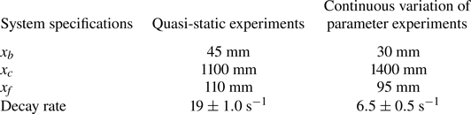
 $1000 \times 500 \times 500$ mm is attached to the end of the combustion chamber. The decoupler ensures that the pressure at the end of the duct is the same as the atmospheric pressure such that fluctuations at the boundary are negligible. The other details of the set-up configuration such as the bluff-body location from the dump plane, combustor length, fuel injection location upstream of the dump plane from the backward facing step (
 $x_f$), and the decay rate of the set-up are tabulated in table 1 for both sets of experiments. The acoustic damping was maintained within limits to ensure repeatability of the experiments (refer to table 1).
Schematic of ( $a$) the experimental set-up of a bluff-body stabilised turbulent combustor and (
 $b$) a cross-section of the combustor showing the backward-facing step, the bluff-body (grey object) and the analysis window (
 ${\rm CH}^*$ window). The different flow regions are labelled as follow: DR denotes the recirculation zone created in the dump plane downstream of the backward-facing step in the dump plane; OSL and ISL denote the outer and inner shear layer; SFR denotes the region of secondary flow recirculation created upstream of the bluff-body and W denotes the wake downstream of the bluff-body. The location of the pressure transducer from the backward facing step (
 $x_p$), length of the combustion chamber (
 $x_c$) and the bluff-body position from the dump plane (
 $x_b$) are marked in the schematic in panel (
 $b$).

System specifications for the turbulent bluff-body stabilised combustor used for experiments where the inlet airflow rate is varied either quasi-statically or continuously. Here,  $x_b$ and
 $x_c$ represent the dimensions of the bluff-body location and combustor length, respectively, as depicted in figure 1. Additionally,
 $x_f$ represents the location of fuel injection location upstream of the dump plane from the backward facing step.

We use liquefied petroleum gas (LPG) (butane 60 % and propane 40 %) as the fuel for combustion and air as the oxidiser. Fuel is injected through the shaft and ejected via four holes of 1 mm diameter. The fuel–air mixture is partially premixed in the burner before being injected into the combustion chamber. The mass flow rates of the inlet fuel and air, measured in SLPM (standard litres per minute), are controlled using mass flow controllers (MFCs). During experiments, we maintain the fuel flow rate constant and vary the air flow rate (flow control parameter), thus varying the Reynolds number ( $Re$) of the inlet fuel–air mixture. The equation used to find
 $Re$ close to the burner position is given by
 $Re = 4\dot {m}D_1/{\rm \pi} \mu D_0^2$, where
 $\dot {m}$ represents the total of the fuel flow rate (
 $\dot {m_f}$) and air-flow rate (
 $\dot {m_a}$),
 $D_0$ denotes the hydraulic diameter of the burner,
 $D_1$ is the circular bluff-body diameter, and
 $\mu$ is the kinematic viscosity of the fuel–air mixture under experimental conditions (Nair et al. Reference Nair, Thampi and Sujith2014). The
 $Re$ of a binary gas mixture was calculated using the dynamic viscosity expression given by Wilke (Reference Wilke1950).
The acoustic pressure fluctuations ( $p'$) in the duct is measured using a piezoelectric pressure transducer. The piezoelectric transducer is mounted on a pressure port (T-joint) that is flush mounted on the combustor wall. To protect the transducer from excess heating from the combustor, a Teflon adapter is used. Further, one shoulder of the T-joint was also provided with a semi-infinite tube 10 m in length to prevent acoustic resonance within the ports, thereby minimising the frequency response of the system. The global unsteady heat release rate (
 $\dot {q}_G$) is measured using a photomultiplier tube (PMT) module. Also, we capture high-speed chemiluminescence images, which are then used to determine the local unsteady heat release rate (
 $\dot {q}(x,y)$) of the flame. The heat release rate fluctuations are calculated at each location as
 $\dot {q}'(x,y)=\dot {q}(x,y) - \langle \dot {q}(x,y)\rangle$, where
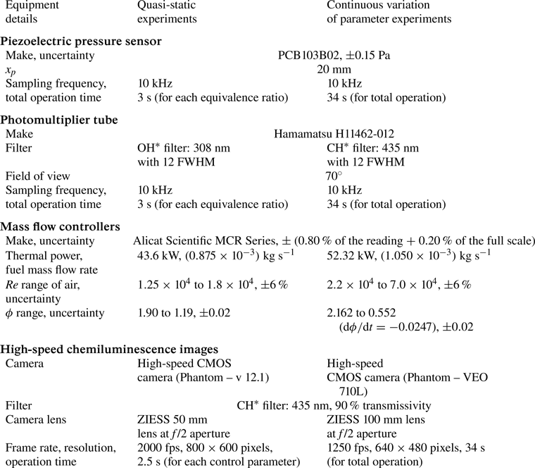
 $\langle \rangle$ denotes a time average. The specification of the instruments used for data acquisition and the operational parameters for both the experimental configurations are tabulated in table 2. During experiments with continuous variations in the airflow rate, the rate of change of the equivalence ratio is
 ${\rm d}\phi /{\rm d}t=-0.0247$. This rate of change of equivalence ratio is close to that typically reported for gas-turbine engines (Davies & Artwork Reference Davies and Artwork1971; Heywood & Mikus Reference Heywood and Mikus1973). Recently, Manikandan & Sujith (Reference Manikandan and Sujith2020) have discussed the need to study rate-dependent bifurcations to determine the thermoacoustic stability map in a turbulent afterburner rig.
Description and specifications of the instruments used for data acquisition during experiments with quasi-static and continuous variation of inlet airflow rate in a turbulent bluff-body stabilised combustor.

Additionally, we performed Mie scattering experiments for the same combustor configuration given in the quasi-static experiment. Mie scattering experiments were performed with olive oil droplets as seeding particles to qualitatively describe the flame front (Shanbhogue et al. Reference Shanbhogue, Shin, Hemchandra, Plaks and Lieuwen2009; Zhang, Shanbhogue & Lieuwen Reference Zhang, Shanbhogue and Lieuwen2010). In the current study, the mean diameter of the seeding particles used is approximately  $1\ \mathrm {\mu }{\rm m}$ at an equivalence ratio of 1.6. A Laskin nozzle is used to seed the olive oil droplets into the incoming air. These droplets scatter light when they pass through a laser sheet, but as the oil droplets traverse through the flame, they evaporate and burn. The boundary of the illuminated area is marked as the flame front, since oil droplets are found exclusively in areas with unburned cold reactants. A Q-switched Nd:YLF laser (527 nm, in single-pulse mode) synchronised with a high-speed camera (Phantom – v 12.1) is used for the Mie scattering experiments. The camera is mounted with a ZEISS 100 mm lens with aperture at
 $f$/2 and outfitted with a short bandpass optical filter (
 $527 \pm 12\ {\rm nm}$) to capture the scattered light from the seeding particles. The camera images
 $51.2\ {\rm mm} \times 36.8\ {\rm mm}$ between the dump plane and the bluff-body onto
 $1024 \times 736$ pixels of the camera sensor. The camera acquires the images at a frame rate of 5000 fps for a duration of 1.8 s.
Figure 1( $b$) shows the window of analysis and a schematic of flow features in the field of the turbulent bluff-body stabilised combustor. As the flow is forced to turn around the backward-facing step and subsequently around the bluff-body, two recirculation zones are formed, one in the dump plane (region DR, figure 1
 $b$) and one in the wake of the bluff-body (region W, figure 1
 $b$), respectively. A secondary flow recirculation denoted as region SFR in figure 1(
 $b$) is created upstream of the bluff-body where the flow along the shaft is forced to turn at a right angle by the bluff-body. Regions denoted as OSL and ISL in figure 1(
 $b$) represent the outer and inner shear layers, respectively. The different flow regions will herewith be referred to in the manuscript by these abbreviations denoted in figure 1(
 $b$). Also, we note that the acoustic pressure signal measured by the transducer at one location represents the acoustic pressure dynamics throughout the analysis window. This is because an acoustic pressure anti-node (maximum of the acoustic mode in space) occurs around the location of the pressure transducer, and we find that the variations in
 $p'$ along the axial direction within our window of analysis are insignificant. Nair (Reference Nair2014) and Sudarsanan et al. (Reference Sudarsanan, Roy, Pavithran, Tandon and Sujith2024) have confirmed this experimentally.
2.1. Typical time series data during the state of intermittency
From quasi-static experiments, we observe the occurrence of intermittency en route the transition from chaotic to periodic acoustic pressure dynamics in our system. Figures 2( $a$) and 2(
 $c$) show the time series of acoustic pressure (
 $p'$) and global heat release rate fluctuations (
 $\dot {q}_G'$), respectively, during the state of intermittency. Bursts of high-amplitude
 $p'$ oscillations are sustained for short epochs amidst aperiodic fluctuations in the acoustic pressure signal (figure 2
 $a$). The
 $p'$ signal exhibits a dominant frequency around 180 Hz, as evident in the spectrogram in figure 2(
 $b$). Also, the
 $\dot {q}_G'$ signal exhibits a dominant frequency at approximately 30 Hz during the epochs of low-amplitude
 $p'$-dynamics, while a band of dominant frequencies appears around 90 Hz during the epochs of high-amplitude
 $p'$ dynamics (see spectrogram in figure 2
 $d$).
(a,c) The time series and (b,d) the corresponding spectrograms showing the time variation of dominant frequencies in the acoustic pressure ( $p'$) and global heat release rate (
 $\dot {q}_G'$) fluctuations during the state of intermittency. The shaded regions in the time series in panels (a,c) correspond to the epochs of high-amplitude
 $p'$ dynamics. Comparing the time series and the spectrograms, we find low-frequency fluctuations in
 $\dot {q}_G'$ are predominant during low-amplitude epochs of
 $p'$ oscillations during the occurrence of intermittency in quasi-static experiments.

Comparing the global time series and spectrograms obtained during the state of intermittency, we can infer that the frequency of the global heat release rate fluctuations ( $\dot {q}_G'$) changes with variations in the amplitude of
 $p'$. However, significant amplitude modulations in
 $p'$ are not present during the state of combustion noise or thermoacoustic instability. In this work, we quantify the inter-dependence between the amplitude of acoustic pressure fluctuations and the frequency of heat release rate fluctuations, and study the spatial pattern of such interactions during the state of intermittency. To do so, we use natural visibility graphs (NVGs) constructed from the heat release rate fluctuations at each location and compare the network properties during high- and low-amplitude
 $p'$ dynamics.
3. Data analysis
3.1. Constructing natural visibility graphs (NVGs)
An NVG (Lacasa et al. Reference Lacasa, Luque, Ballesteros, Luque and Nuno2008; Nuñez et al. Reference Nuñez, Lacasa, Gomez and Luque2012; Zou et al. Reference Zou, Donner, Marwan, Donges and Kurths2019) is a tool to encode the features of a time series onto a complex network comprising nodes and links. Each time stamp is considered as a node. A connection is established between two nodes if a straight line drawn between the corresponding data points does not intersect any other intermediate data point, i.e. the two nodes are ‘visible’ to each other. Mathematically, node  $i$ and
 $j$ of time series
 $y(t)$ will be connected to each other if every intermediate node
 $n$ satisfies the condition:
 \begin{equation} y(t_n) < y(t_j) + (y(t_i) - y(t_j)) \frac{t_j - t_n}{t_j - t_i}. \end{equation}
The network is represented by an adjacency matrix  $\boldsymbol {A} = [a_{ij}]$ of size
 $N \times N$, where
 $N$ is equal to the total number of time stamps in the time series. Elements of
 $\boldsymbol {A}$ are
 $a_{ij} = 1$, if there exists a link between nodes
 $i$ and
 $j$, else
 $a_{ij} = 0$. Therefore, the adjacency matrix
 $\boldsymbol {A}$ for NVG is symmetric, and the network is unweighted and undirected. Note that the network generated is invariant under the scaling transformation of the time series (Lacasa et al. Reference Lacasa, Luque, Ballesteros, Luque and Nuno2008).
NVG captures the frequency modulation (FM) in a uniformly sampled time series (Iacobello, Scarsoglio & Ridolfi Reference Iacobello, Scarsoglio and Ridolfi2018; Iacobello et al. Reference Iacobello, Ridolfi and Scarsoglio2021a). Consider a typical time series exhibiting FM and the corresponding NVG shown in figures 3( $a$) and 3(
 $b$), respectively. Note that the visibility of a node close to the trough is restricted by the neighbouring peaks in the time series. For a time series with uniform sampling rate, one cycle of a high-frequency periodic oscillation has a smaller time period and contains a lower number of time stamps (nodes) compared with that of a low-frequency oscillation. For example, a node in a high-frequency oscillation cycle can connect to a lower number of nodes as compared with a node in low-frequency oscillation. Thus, the variation in the number of connections of a node quantifies the variation in the frequency of the time series. The number of connections of a node
 $i$ is called its degree, which is expressed as
 $k_i = \sum _{j = 1} ^{N} a_{ij}$.
( $a$) A typical time series (
 $y(t)$) exhibiting frequency modulation and (
 $b$) its corresponding natural visibility graph (NVG) with time stamps as nodes. The blue and red stems at each time stamp indicate the amplitude of
 $y$ at that instant. Links between nodes are indicated by grey lines and determined by visibility algorithm. From the figure, it is evident that in the epochs of low-frequency dynamics (blue parts of the time series), the density of connections between nodes in the NVG is higher than that during epochs of high-frequency variations. Thus, the variations in the number of connections of a node in NVG captures the variation in frequency of a time series.

Compare the number of connections between two consecutive peaks during low- and high-frequency dynamics in figure 3( $b$). Clearly, the average degree of a node in the high-frequency epoch is less than that of a node in the low-frequency epoch. On comparing the average degree of nodes during different epochs, one can infer the frequency modulation in the signal. Recently, this feature of NVG was used to study frequency modulation in the streamwise and spanwise components of velocity fluctuations in wall-bounded turbulence resulting from the interaction between small- and large-scale flow structures (Iacobello et al. Reference Iacobello, Ridolfi and Scarsoglio2021a). Here, we apply this method (Iacobello et al. Reference Iacobello, Ridolfi and Scarsoglio2021a) to study interactions in the form of cross-variable amplitude–frequency coupling arising between the acoustic and heat release rate signals.
3.2. Cross-variable conditionally averaged degree from natural visibility graphs
From the spectrogram in figure 2( $b$), we notice that the amplitude of the dominant frequency of the acoustic pressure signal is significant during the epochs of high-amplitude periodic oscillations as compared with that of low-amplitude fluctuations in
 $p'$. We identify epochs of high- and low-amplitude
 $p'$ dynamics using short-time Fourier transform performed on non-overlapping windows of the time series of
 $p'$. The size of a window
 $w$ corresponds to
 $L=5$ cycles of the dominant acoustic mode. We find the amplitude of the frequency of the dominant mode (
 $A_{DM}^w$) from the short-time Fourier transform for each window
 $w$. Then, we set a threshold on these amplitudes of dominant frequency across all windows as
 $A_\tau = 15\,\%$ of
 ${\max } (A_{DM}^w)$. Then, any window
 $w$ for which
 $A_{DM}^w>A_\tau$ is identified as a window of high-amplitude
 $p'$ dynamics, else as an epoch of low-amplitude
 $p'$ dynamics. In Appendix A, we show that the spatial pattern of cross-variable amplitude–frequency coupling obtained using this approach remains qualitatively similar for small variations in
 $L$ and
 $A_\tau$.
To identify the spatial pockets of frequency modulation in heat release rate dynamics, we construct an NVG of  $\dot {q}'(x,y)$ fluctuations at each location in the flow field. Then, we find the conditionally averaged degree of nodes included in all those windows which are identified as epochs of high-amplitude (or low-amplitude)
 $p'$ dynamics using the criterion discussed above, and denote it as
 $K_h$ (or
 $K_l$) as given by (3.2). Thus,
 \begin{equation} \left.\begin{gathered}
K_{h}(x,y) = \frac{1}{N_h}\sum_{j=1}^{N} (k_j(x,y)|\,j\in w:
A_{DM}^w>A_\tau),\\ K_{l}(x,y) =
\frac{1}{N_l}\sum_{j=1}^{N} (k_j(x,y)|\,j\in w: A_{DM}^w<
A_\tau), \end{gathered}\right\}
\end{equation}
where  $(x,y)$ denotes a spatial location,
 $N_h$ and
 $N_l$ are the total number of nodes (time stamps) during the high- and low-amplitude epochs in the time series of
 $p'$, respectively. Also,
 $k_j$ is the degree of the
 $j\textrm {th}$ node,
 $j\in w$ denotes that
 $w$ is the short-time window containing node
 $j$, and
 $N$ is the total number of nodes. Note that
 $K_h$ and
 $K_l$ are conditional averages of degree of nodes in the NVG of
 $\dot {q}'$ conditioned over the amplitude of acoustic pressure oscillations, and are thus called the conditional average degree.
Next, we compute the ratio  $K_{lh}(x,y) = {K_l(x,y)}/{K_h(x,y)}$, as proposed by Iacobello et al. (Reference Iacobello, Ridolfi and Scarsoglio2021a), to quantify changes in the frequency of
 $\dot {q}'$ at a location
 $(x,y)$ with variation in the amplitude of
 $p'$. Note that Iacobello et al. (Reference Iacobello, Ridolfi and Scarsoglio2021a) have shown that the ratio of conditionally averaged degrees obtained from the NVG reflects frequency modulation alone, even if both amplitude and frequency modulation occur in a signal.
From figure 3, we understand that a greater average degree in a time window means a lower frequency of oscillations in that window. Then, if  $K_{lh}(x,y)>1$, i.e.
 $K_l(x,y)>K_h(x,y)$, the frequency of
 $\dot {q}'$ fluctuations at location
 $(x,y)$ is lower during the epochs of low-amplitude
 $p'$ dynamics as compared with that for epochs of high-amplitude
 $p'$ dynamics. Thus,
 $K_{lh}(x,y)>1$ signifies that, on average, the frequency of
 $\dot {q}'$ fluctuations at location
 $(x,y)$ increases when the amplitude of
 $p'$ oscillations increases, and we refer to this condition as positive frequency modulation (FM). In contrast, if
 $K_{lh}(x,y)<1$, we infer that, on average, the frequency of
 $\dot {q}'$ fluctuations at location
 $(x,y)$ decreases when the amplitude of
 $p'$ oscillations increases, and we refer to this condition as negative FM.
The method using a cross-variable conditionally averaged degree of the NVG introduced here helps capture simultaneous co-evolution of and coupling between the frequency of one variable and amplitude of another. This approach is advantageous compared with conventional spectrogram analysis, where frequency modulation in one variable is detected independent of other variables in the system.
4. Results
4.1. Occurrence of intermittency during quasi-static experiments
In quasi-static experiments, we vary the flow control parameter such that fully developed dynamical states are achieved at each control parameter. As described in § 2, we observe a dynamical transition in the acoustic pressure fluctuations from chaotic to periodic dynamics through a state of intermittency. Here, we analyse the cross-variable coupling between the acoustic pressure and the heat release rate fluctuations during the state of intermittency using the method described in § 3. Figure 4( $a$) shows the normalised time series of the acoustic pressure (
 $p'$) and the global heat release rate (
 $\dot {q}_G'$) fluctuations obtained during this state. Each time series is normalised by its maximum value. Figure 4(
 $b$) shows the spatial pattern of the instantaneous heat release rate (
 $\dot {q}(x,y)$) corresponding to the points (I–V) marked in the time series of
 $\dot {q}_G'$ in figure 4(
 $a$). Distinct spatial patterns of heat release rate occur during high- and low-amplitude
 $p'$ dynamics.
( $a$) Normalised time series of acoustic pressure (
 $p'$) and global heat release rate (
 $\dot {q}_G'$) fluctuations, during the state of intermittency observed in quasi-static experiments in a turbulent bluff-body stabilised combustor. (
 $b$) The spatial pattern of heat release rate (
 $\dot {q}(x,y)$) during high-amplitude (I–II) and low-amplitude (III–V) acoustic pressure dynamics corresponding to the points marked in the time series plot in panel (
 $a$). The strength and location of significant heat release are different during epochs of high- and low-amplitude amplitude
 $p'$ oscillations.

When  $\dot {q}_G'$ is at a local maximum during the high-amplitude
 $p'$ dynamics (see figure 4
 $b$-I), the heat release rate is very high specifically in the inner shear layer and regions downstream of the bluff-body (ISL and W regions in figure 1). When
 $\dot {q}_G'$ is at a local minimum during the high-amplitude
 $p'$ dynamics (see figure 4
 $b$-II), the heat release rate is significant around the bluff-body, particularly in the inner shear layer and in the region of secondary flow recirculation (i.e. regions ISL and SFR, as shown in figure 1
 $b$, respectively). However, when
 $\dot {q}_G'$ is maximum during the low-amplitude
 $p'$ dynamics (see figure 4
 $b$-III,IV), the heat release rate is significant in the ISL, OSL and SFR regions. Finally, when
 $\dot {q}_G'$ is minimum during the low-amplitude
 $p'$ dynamics, the strength of heat release rate reduces and is significant predominantly in the SFR and ISL regions (see figure 4
 $b$-V).
Figure 5 shows the oil Mie scattering images delineating the flame front and the anchoring position during the state of intermittency obtained during quasi-static experiments in the combustor. During epochs of aperiodic fluctuations in  $p'$ (such as in figure 5
 $e$), the flame anchors predominantly at two locations, one in the OSL close to the backward-facing step and another along the shaft in the ISL region upstream of the bluff-body as evident in figures 5(
 $a$)–5(
 $d$). The flame can also anchor in the SFR region, although rarely, during such aperiodic epochs (as in figure 5
 $a$). Further, small-scale distortions are evident along the flame front in the OSL, ISL and SFR regions (see figure 5a–d).
(a–d) Oil Mie scattering images and ( f–i) delineating the flame-anchoring locations and flame front during epochs of (e) aperiodic and ( j) periodic fluctuations in  $p'$, respectively, during the state of intermittency obtained in quasi-static experiments in a turbulent bluff-body stabilised combustor. The flame anchors predominantly in the dump plane at the edge of the outer shear layer. Along the shaft holding the bluff-body, the flame anchoring extends into the secondary flow recirculation region during periodic epochs but remains restricted upstream during aperiodic epochs of intermittency.

During epochs of high-amplitude periodic oscillations in  $p'$, the flame anchors in an extended region along the shaft. The flame-anchoring location in the OSL region close to the backward-facing step is similar during both periodic and aperiodic epochs (see figure 5f–i). However, the flame also anchors often in the SFR region during the epochs of periodic fluctuations in
 $p'$ (see figure 5g,h). The flame front in the OSL region exhibits large-scale distortions induced by large-scale coherent structures shed during this epoch (see figure 5f,g,i). Also, the flame anchors in the ISL region close to the shaft and the flame front in the ISL region exhibits small-scale distortions that merge with the flame anchored in the SFR region (see figure 5f–h). The turbulent flame front extends and oscillates between the OSL and recirculation zone in the dump plane (DR region) and the part of inner shear layer above and downstream of the bluff-body.
Figures 6( $a$) and 6(
 $b$) show the time series of global heat release rate (
 $\dot {q}_G'$) and acoustic pressure (
 $p'$) oscillations, respectively. The time series of
 $p'$ is partitioned into epochs of low- and high-amplitude oscillations using short-window fast Fourier transform, as described in § 3.2. The epochs of high-amplitude
 $p'$ dynamics are shaded grey in figures 6(
 $a$) and 6(
 $b$). We construct NVGs from the time series of global heat release rate fluctuations (
 $\dot {q}_G'$) as described in § 3.1. Then, we compute the average degree (
 $\langle k \rangle$) over short time windows corresponding to five acoustic cycles, as shown by the blue curve in figure 6(
 $a$). Clearly, the value of
 $\langle k \rangle$ is relatively lower during epochs of high-amplitude
 $p'$ dynamics, as compared with the epochs of low-amplitude
 $p'$ dynamics. Remember, a higher average degree of NVG in an epoch means a lower frequency of oscillations in that epoch of the corresponding time series (§ 3.2). Thus, we infer that the frequency of
 $\dot {q}_G'$ is higher during epochs of high-amplitude
 $p'$ dynamics as compared with low-amplitude
 $p'$ dynamics.
Time series of ( $a$) global heat release rate fluctuations (
 ${\dot {q}'_G}$, red curve), the variation of short-time averaged degree (
 $\langle k \rangle$, blue curve) obtained from the NVG of
 ${\dot {q}'_G}$, and (
 $b$) the time series of acoustic pressure (
 $p'$). The shaded regions represent epochs of high-amplitude
 $p'$ dynamics. (
 $c$) Spatial distribution of the ratio of conditionally averaged degree during low- and high-amplitude
 $p'$ dynamics,
 $K_{lh}$, during the state of intermittency obtained during quasi-static experiments in a turbulent bluff-body stabilised combustor. The average degree
 $\langle k \rangle$ (in panel
 $a$) is lower and hence the frequency of
 $\dot {q}_G'$ is higher during epochs of high-amplitude
 $p'$ oscillations as compared with that in low-amplitude
 $p'$ fluctuations. Spatially,
 $\dot {q}'$ exhibits positive frequency modulation specifically in the outer shear layer, parts of the inner shear layer and secondary flow recirculation zone, which are also the regions of flame anchoring, and negative frequency modulation in spatial pockets in the dump plane, which are also the regions of significant flame-front distortion.

Next, we construct the NVG of local heat release rate fluctuations ( $\dot {q}'(x,y,t)$) at each location
 $(x,y)$ in the combustor and compute
 $K_{lh}$, that is, the ratio of short-time average conditional degree during low- and high-amplitude
 $p'$ dynamics (as discussed in § 3.2). Note that
 $K_{lh}>1$ at a location implies positive frequency modulation (FM), that is, frequency of
 $\dot {q}'$ increases with the amplitude of
 $p'$. We find that positive FM occurs in the regions associated with flame anchoring during epochs of high-amplitude
 $p'$ dynamics, namely the OSL and SFR regions and part of the ISL region close to the shaft (compare red regions in figure 6(
 $c$) with the flame in figure 5f–i).
Also, negative FM ( $K_{lh}<1$) occurs in a spatial pocket in the dump plane close to the OSL which is associated with large-scale flame-front distortions during the epochs of high-amplitude
 $p'$ dynamics (compare the blue pocket in the DR region in figure 6
 $c$ with figure 5f,g). Negative FM also occurs in pockets of the ISL and wake (W region) downstream of the bluff-body and close to the top wall of the combustor. There is no significant FM in
 $\dot {q}'$ and
 $K_{lh}\approx 1$ in the core of the turbulent flame in the ISL region very close to the shaft of the bluff-body.
In summary, we find that the  $\dot {q}'$ fluctuations exhibit lower frequency in the regions associated with flame flapping, and higher frequency in the regions of flame anchoring during high-amplitude
 $p'$ dynamics as compared with low-amplitude
 $p'$ dynamics. Our finding implies that a unique spatial pattern of cross-variable amplitude–frequency coupling emerges during the state of intermittency. This pattern of interaction can be understood in terms of the physical processes, as follows.
During the state of intermittency, high-amplitude periodic  $p'$ oscillations are sustained for short epochs owing to flame–acoustic interactions. High-frequency fluctuations in
 $\dot {q}_G'$ during epochs of high-amplitude
 $p'$ dynamics (as detected in figure 6
 $a$) imply that the aggregate heat release rate fluctuations are possibly more often in phase with the acoustic pressure fluctuations, thus sustaining the periodic
 $p'$ dynamics. However, due to acoustic damping and turbulence in the flow and flame dynamics, high-amplitude
 $p'$ fluctuations are not sustained for very long.
We find that during epochs of high-amplitude  $p'$ oscillations, large coherent structures form and shed in the dump plane and convect downstream from the top of the bluff-body into the wake (George et al. Reference George, Unni, Raghunathan and Sujith2018). The size and shedding frequency of these vortices depend on fluctuations in the acoustic field (Chu & Kovásznay Reference Chu and Kovásznay1958; Matveev & Culick Reference Matveev and Culick2003). Large vortices delay mixing as they entrain and trap the unburnt reactants. Combustion occurs after the entrained reactants mix completely with hot products contained in the recirculation zones, and leads to sudden heat release. Sometimes these vortices can hit the bluff-body or the walls of the combustor and break into smaller vortices enhancing the mixing (Schadow & Gutmark Reference Schadow and Gutmark1992). The large vortices are shed almost periodically and distort the flame as they convect downstream during epochs of high-amplitude
 $p'$ dynamics (George et al. Reference George, Unni, Raghunathan and Sujith2018).
A larger vortex means a larger scale of the flame-front distortion. Such flame-front distortion causes flapping of the free end of the flame and induces low-frequency oscillations in the  $\dot {q}'$ dynamics during these epochs. In contrast, during low-amplitude
 $p'$ fluctuations, the smaller vortices introduce small-scale distortions in the flame inducing comparatively higher-frequency fluctuations in the free end of the flame. As a result, we find negative FM in local heat release in regions associated with flame-front distortion and flapping, that is, in the spatial pockets in the dump plane and in the wake region close to the top wall of the combustor (blue pockets in figure 6
 $c$).
However, the large coherent structures discussed above do not perturb the flow and flame in the ISL and SFR regions close to the bluff-body shaft and in the OSL region close to the backward-facing step. Hence, these are the regions of flame anchoring during high-amplitude periodic  $p'$ oscillations during the state of intermittency. When the amplitude of
 $p'$ oscillations is high, the acoustic field perturbations induce stronger excitation to the flow and flame dynamics. As a result, the turbulent flow and flame dynamics are excited at higher frequencies during epochs of high-amplitude
 $p'$ compared with low-amplitude
 $p'$ dynamics in these regions. Hence, we find positive FM in the regions where the flame anchors during high-amplitude
 $p'$ dynamics, that is, the OSL, ISL and SFR regions.
The frequency of local heat release rate fluctuations varies in time differently at distinct locations. As a result, the phase between the acoustic pressure and local heat release rate fluctuations shifts dynamically and alters the spatial pattern of thermoacoustic power generation. In Appendix B, using the spatial variation of Rayleigh index (a measure of thermoacoustic power), we show that the locations of positive FM are associated with stronger sources or weaker sinks of thermoacoustic power during high-amplitude  $p'$ dynamics.
We note that not only does the coupling between  $p'$ and
 $\dot {q}'$ dynamics determine the system dynamics, but the state of the system also determines the strength and pattern of these interactions. During the state of thermoacoustic instability, the effect of system damping and turbulence is dominated by the nonlinear feedback between acoustic, combustion and fluid dynamics leading to a self-sustained high-amplitude acoustic pressure dynamics. Evidently, such high-amplitude
 $p'$ oscillations are associated with self-sustained high-frequency oscillations in the heat release rate dynamics (George et al. Reference George, Unni, Raghunathan and Sujith2018). Our analysis during the state of intermittency reveals a spatial pattern of positive and negative frequency modulations with the amplitude of
 $p'$ and thus highlights the interactions that are possibly responsible for the frequency shift in
 $\dot {q}'$ as the system dynamics transitions from chaos to order as reported by Pawar et al. (Reference Pawar, Seshadri, Unni and Sujith2017).
4.2. Occurrence of intermittency during continuous variation of flow control parameter
We perform a set of experiments in a turbulent bluff-body stabilised combustor where the air flow rate is varied continuously at a finite rate as described in § 2. As the inlet air flow rate is varied at a finite rate, the Reynolds number ( $Re$) of the inlet flow increases linearly while the equivalence ratio (
 $\phi$) decreases linearly. The time series of acoustic pressure fluctuations (
 $p'$), the global heat release rate (
 $\dot {q}_G$) and the spatial pattern of instantaneous heat release rate (
 $\dot {q}(x,y)$) are shown in figure 7. The time series of
 $p'$ and
 $\dot {q}_G$ exhibit a dynamical transition from the state of intermittency to self-sustained limit cycle oscillations as
 $Re$ increases continuously. Also, from figures 7(
 $a$) and 7(
 $b$), we observe that the average amplitude of
 $p'$ and
 $\dot {q}_G$ oscillations increase continuously with monotonic increase in
 $Re$.
( $a$) Time series of acoustic pressure fluctuations (
 $p'$, blue curve), Reynolds number of inlet fuel–air mixture (
 $Re$, red line) and (
 $b$) global heat release rate (
 $\dot {q}_G$) obtained from experiments in a turbulent bluff-body stabilised turbulent combustor when the inlet mass flow rate of air (
 $\dot {m}_a$) is varied at a finite rate while the mass flow rate of fuel (
 $\dot {m}_f$) is maintained at a constant value. (
 $c$) The spatial heat release rate (
 $\dot {q}(x,y)$) observed in the combustor shown in rows (A–C) corresponding to each of the insets (A–C) in the time series of
 $\dot {q}_G$ in panel (
 $b$). The labels (I–V) for each row correspond to points (I–V) labelled in the time series in each of the insets in panel (
 $b$). The rows A, B, C represent the spatial heat release pattern during the occurrence of low-, moderate- and high-amplitude intermittency, respectively. The average strength of heat release rate increases with
 $Re$ as evident in the time series of
 $\dot {q}_G$ as well as spatial distribution of
 $\dot {q}$. Further, the spatial pattern of significant heat release varies significantly with the average increase in
 $p'$ as well as with amplitude variations during intermittent oscillations in
 $p'$ during short time windows.

We decipher the relation between the flame and acoustic field dynamics during the dynamical transition induced by a continuous variation in the control parameter. To do so, we divide the entire data into short time-windows of  $T_w=0.6$ s. Note that the average increase in the amplitude of
 $p'$ within one time frame
 $T_w$ is negligible compared with the amplitude variation between periodic and aperiodic fluctuations in
 $p'$ during that window (see insets A–C in figure 7). Hence, we analyse each of these time-windows similar to that done for quasi-static experiments in the previous subsection. For each time frame (
 $T_w=0.6$ s is equivalent to
 $68$ cycles of the dominant acoustic mode), we compute the short-window fast Fourier transform over a smaller time period corresponding to five cycles of the dominant acoustic mode (
 $L=5$ as described in § 3.2). We then classify the epochs of high- and low-amplitude
 $p'$ dynamics within each time frame using the method described in § 3.2.
Figure 8 shows the spatial distribution of  $K_{lh}$ during consecutive time windows (each of
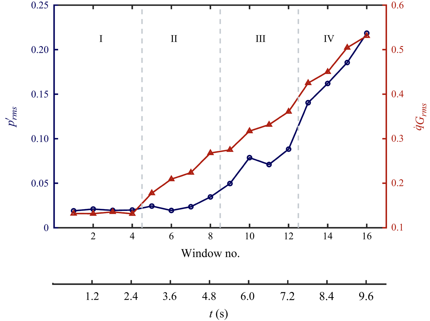
 $0.6$ s). Here, we classify the dynamical transition observed in experiments into three regimes, namely, low, moderate and high amplitude intermittency dynamics (for example, insets A–C in figure 7(a,b), respectively) that occur prior to the onset of high-amplitude self-sustained periodic oscillations. We observe that the acoustic pressure, global and local heat release rate dynamics are distinct during these regimes. To demarcate these dynamical regimes quantitatively, we use the variations in
 $p'_{rms}$ and
 $\dot {q}_{G_{rms}}$ calculated over each time window of
 $T_w=0.6$ s, as discussed in Appendix D. In Appendix E, we show that the flame–acoustic interactions inferred during each dynamical regime are not sensitive to small changes in the value of
 $T_w$.
Spatial distribution of the ratio of conditional degree during low- and high-amplitude  $p'$ dynamics,
 $K_{lh}$, obtained from the NVG of
 $\dot {q}'$ dynamics for consecutive time windows (each of
 $T_w=0.6$ s) during dynamical transition in a turbulent bluff-body stabilised combustor when the air flow rate is varied at a finite rate. Here, panels (I–IV), (V–VIII) and (IX–XII) correspond to the epochs when the average amplitude of acoustic pressure oscillations is low, moderate and high during the occurrence of intermittency, respectively. The classification of the average amplitude into these three ranges is made qualitatively. Regions of strong positive and negative frequency modulation are evident during the occurrence of intermittency dynamics in experiments involving continuous variation of the airflow rate. A remarkable shift in such regions of positive and negative frequency modulation (FM) is observed with increase in the average amplitude of
 $p'$ during the state of intermittency. Variations in regions of positive and negative FM occur due to dynamically changing locations of flame anchoring and flame-front distortions.

4.2.1. Low-amplitude intermittency regime
At low  $Re$, the time series of
 $p'$ and
 $\dot {q}_G$ exhibit low-amplitude intermittency dynamics with very low-amplitude aperiodic fluctuations interspersed between short epochs of relatively high-amplitude periodic oscillations (see inset A in figure 7a,b). During our experiments, we observe that the flame is anchored predominantly in the OSL region close to the backward-facing step. The free end of the turbulent flame exhibits significant oscillations between the OSL and ISL regions and the dump plane (DR region). Thus, we find that significant heat release occurs predominantly in the ISL region above and downstream of the bluff-body and in the OSL (see figure 7(
 $c$)-A(I–V) and figure 12(
 $a$-I–IV) in Appendix C).
The spatial distribution of  $K_{lh}$ obtained during such low-amplitude intermittency dynamics is shown in figure 8(
 $a$). We find that positive FM (
 $K_{lh}>1$) occurs predominantly in the OSL and also in a spatial pocket in the dump plane (see figure 8
 $a$-II,IV). Further,
 $K_{lh}>1$ in parts of the ISL above the bluff-body and also in the wake downstream of and very close to the bluff-body (see figure 8
 $a$-I,III,IV). In summary, positive FM occurs predominantly in the recirculation zones in the dump plane and wake of the bluff body (DR and W regions) and also in the location of flame anchoring, that is the OSL.
However,  $K_{lh}<1$ (signifying negative FM) in certain pockets in the dump plane aligned adjacent to the OSL (see figure 8
 $a$-II,IV) and in pockets in the wake close to the top wall of the combustor (see figure 8
 $a$-I,III). These regions are associated with the free oscillating end of the flame and negative FM is induced due to flame distortion by coherent structures. Note that the coherent structures shed are relatively smaller in size and the epochs of periodic dynamics are relatively shorter during low-amplitude intermittency dynamics compared with other dynamical regimes. As a result, the flame distortion by vortices occurs in a small spatial extent and for shorter epochs. Hence, we find that negative FM occurs in small pockets associated with flame distortion that occurs typically in the dump plane and close to the top wall of the combustor downstream of the bluff-body.
4.2.2. Moderate-amplitude intermittency regime
Insets B in figure 7(a,b) show the time series of  $p'$ and
 $\dot {q}_G$ during moderate-amplitude intermittency dynamics that occurs when
 $Re$ of the inlet flow increases continuously in experiments. During our experiments, we observe that the flame anchors in the dump plane and OSL close to the backward-facing step and also along the shaft of the bluff-body. Close to the shaft, the flame anchors primarily in the ISL region upstream of the SFR region and the flame front exists primarily in the OSL, ISL and SFR regions. However, sometimes, the flame may also anchor in the SFR region and then the flame front oscillates in the ISL and W regions above and close to the bluff-body.
We observe that when  $p'$ exhibits relatively high-amplitude periodic dynamics, instantaneous heat release rate is most significant in the SFR region and ISL above the bluff-body (see figure 7
 $c$-B(III–V)). However, when
 $p'$ exhibits relatively low-amplitude aperiodic fluctuations, significant heat release occurs in the SFR, OSL and ISL regions (see figure 7
 $c$-B(I,II)). Detailed inferences about the flame dynamics are presented using the spatial pattern of mean heat release rate in Appendix C.
Figure 8( $b$) show the spatial distribution of
 $K_{lh}$ obtained during moderate-amplitude intermittency dynamics. Spatial pockets in the ISL close to the top wall of the combustor exhibit negative FM (figure 8
 $b$-V–VIII). Intriguingly, we find that negative FM occurs in the OSL in figure 8(
 $b$-V,VII) but positive FM occurs in spatial pockets in the OSL in figure 8(
 $b$-VI,VIII). In figure 8(
 $b$-VI), we find that
 $K_{lh}>1$ along the shaft, whereas in figure 8(
 $b$-V,VII)
 $K_{lh}\approx 1$ in the SFR region close to the shaft. Also, SFR region exhibits positive FM for some short epochs such as in figure 8(
 $b$-VIII).
We conjecture that such alternating pattern of positive and negative FM occurs due to the appearance of large coherent structures and variations in flame-anchoring position observed in experiments. Compared with the low-amplitude intermittency regime, epochs of periodicity are longer, the vortices shed in the dump plane are relatively larger, the mean flow velocity is greater and the typical local flow time scale is smaller during the moderate-amplitude intermittency regime. Thus, the flame is able to anchor in the dump plane only for short epochs and tries to anchor in SFR region during other epochs. Further, flame-front distortion occurs predominantly in the OSL region or in some spatial pockets adjacent to OSL in the dump plane. The flame distortion extends well into the OSL region owing to the larger size vortices formed in the dump plane during this dynamical regime. As a result, we find negative FM in the OSL during some time windows (figure 8 $b$-V,VII).
However, when the flame anchors close to the backward facing step, we obtain patches of positive FM in the OSL, as shown in figure 8( $b$-VI,VIII). Further, the flame anchors not only in the OSL, but also in the SFR region as the flame is perturbed by relatively large vortices shed in the DR and OSL region. As a result, positive FM is observed in the ISL and SFR regions close to the shaft, such as in figure 8(
 $b$-VI,VIII). Furthermore, flame-front oscillations are prominent in the ISL region above and downstream of the bluff-body. Hence, we find negative FM in these regions. The effect of large coherent structures on the flame anchoring and flame-front distortion becomes more prominent during high-amplitude intermittency dynamics as discussed below.
4.2.3. High-amplitude intermittency regime
With further continuous increase in  $Re$, we observe high-amplitude intermittency dynamics characterised by long epochs of high-amplitude periodic oscillations interspersed with short epochs of low-amplitude aperiodic fluctuations in
 $p'$. We observe in our experiments that the flame anchors primarily along the shaft of the bluff-body and not close to the backward-facing step any longer. Moreover, the flame-anchoring location keeps shifting dynamically along the shaft. Such shifts in the flame-anchoring location along the shaft appear to occur more frequently during the high-amplitude (compared with moderate-amplitude) intermittency regime. The flame anchors either upstream of the SFR or in the SFR region close to the shaft. We obtain very high heat release rate in the OSL, ISL and SFR regions (refer to figure 7
 $c$-C(I–V)). Also, the turbulent flame extends downstream of the bluff-body and significant heat release occurs in the wake region (evident in figure 7
 $c$-C(V)). The flame dynamics during this dynamical regime is discussed further with respect to mean heat release rate during short time frames in Appendix C.
The spatial distribution of  $K_{lh}$ obtained during the occurrence of high-amplitude intermittency is shown in figure 8(
 $c$). The pattern of frequency modulation is distinct in each time frame. In figure 8(
 $c$-IX), we find
 $K_{lh}>1$ in a spatial pocket in the ISL very close to the shaft of the bluff-body extending upwards into the OSL region. Moreover, we find
 $K_{lh}<1$ in the SFR region and in the region above the bluff-body in figure 8(
 $c$-IX). Further, in figure 8(
 $c$-X,XI), we do not find any coherent spatial pockets exhibiting positive FM. Instead, we find
 $K_{lh}<1$ in most regions in the flow field. Specifically, negative FM occurs in the SFR, OSL and ISL regions and in a large spatial pocket spanning across the recirculation zone in the dump plane (DR region). Finally, in figure 8(
 $c$-XII), we find negative FM occurs predominantly in the DR and OSL regions upstream and the ISL and W regions above and downstream of the bluff-body. We also find positive FM in the SFR region during the time-frame shown in figure 8(
 $c$-XII). Furthermore, incoherent patches of both positive and negative FM occur in very small pockets at scattered locations in the OSL and ISL region upstream of the bluff-body, evident in figure 8(
 $c$-X–XII).
Note that the location of flame anchoring is stable if the mean flame front emerges from and remains attached to this location and if the flow dynamics entrains unburnt fuel alongside hot products across the flame front. However, as vortices form and convect downstream, the mixing of reactants and hot products is delayed and the primary location of recirculation changes dynamically with the convection of each large coherent structure. As the mean flow velocity increases owing to continuous variations in the inlet airflow rate, much larger vortices are shed almost periodically in the dump plane and the frequency of local velocity fluctuations increases (that is, the typical flow time scale decreases). Moreover, the flame–acoustic interactions become stronger as the amplitude of acoustic pressure oscillations increase. Very high-amplitude  $p'$ oscillations also imply strong acoustic velocity fluctuations which perturb the flame along with the turbulent flow dynamics. The flame anchors in the SFR region during short epochs due to the presence of very large vortex that forms in the dump plane and the OSL region. High-frequency fluctuations in the local velocity perturb the flame anchoring in the SFR region. Thus, when the large vortex convects downstream or dissipates and until the next one appears, the flame tries to anchor upstream of the SFR region along the shaft. Hence, the flame-anchoring location appears to oscillate to and fro along the shaft during this dynamical regime. The flame distortion occurs in a much larger spatial extent during such epochs of high-amplitude
 $p'$ dynamics.
Hence, large spatial pockets in the OSL and DR regions exhibit negative FM (such as in figure 8 $c$-X–XII) due to low-frequency oscillations induced in
 $\dot {q}'$ by the large-scale flame-front distortions. Further, we observe that negative FM occurs in regions close to the top wall of the combustor and downstream of the bluff-body (see figure 8
 $c$-IX–XII). As the large vortex convects downstream and hits the top wall of the combustor, it dissociates into relatively smaller vortices which further distort the flame in the wake of the bluff-body. Such flame distortions induce negative FM in these downstream locations. Since the flame anchors along the shaft, one might expect positive FM in most regions along the shaft. However, the location of flame anchoring keeps oscillating to and fro along the shaft. Evidently, our method identifies the prominent location of flame anchoring during certain time windows such as figure 8(
 $c$-IX,XII) since positive FM is associated with flame-anchoring locations.
When the flame anchors for comparatively longer epochs in the SFR region during a time frame (of  $0.6$ s), we obtain positive FM in a small pocket in the SFR region (see figure 8
 $c$-XII). However, when the flame anchors mostly upstream of the SFR region in a certain time frame, we observe positive FM as seen in figure 8(
 $c$-IX). However, due to continual shifting of the flame-anchoring location along the shaft during certain epochs, a low-frequency component is introduced in the local heat release rate oscillations. Also, due to shifts in the flame-anchoring location, the SFR region experiences flame-front oscillations for certain epochs which induce low-frequency fluctuations in heat release rate during high-amplitude
 $p'$ dynamics. Hence, we obtain negative FM in the SFR and ISL regions close to the shaft (see figure 8
 $c$-IX–XI).
Finally, we note that a very large flame-front distortion can also comprise small flame-front distortions within it owing to the interaction of the flame front with coherent structures of multiple length scales in the underlying turbulent flow and with the acoustic field fluctuations. A detailed quantification of such small-scale structures in the flame front within large-scale flame distortion was done by Raghunathan et al. (Reference Raghunathan, George, Unni, Midhun, Reeja and Sujith2020) using multifractal analysis. They also showed quantitatively that the effect on dynamics of the small-scale structures is more dominant than that of the large-scale coherent structures. We conjecture that incoherent patches of positive and negative FM appearing in the ISL and OSL regions are due to the multi-scale flame-front distortion inducing spatially incoherent frequency modulations in the local heat release rate dynamics.
5. Conclusion
Dynamical transition from chaos to self-sustained order via the route of intermittency in turbulent thermoacoustic systems is well known. In this work, we describe the rich spatial pattern of a unique cross-variable amplitude–frequency coupling between the co-evolving variables acoustic pressure ( $p'$) and local heat release rate dynamics (
 $\dot {q}'$) in the system, during the state of intermittency obtained when the mass flow rate of the inlet air is varied (
 $a$) quasi-statically and (
 $b$) continuously at a finite rate in a turbulent bluff-body stabilised combustor. Towards this purpose, we apply the method proposed by Iacobello et al. (Reference Iacobello, Ridolfi and Scarsoglio2021a) using a natural visibility algorithm (NVG) to detect frequency modulation (FM). We use this method to study cross-variable amplitude–frequency coupling between the acoustic and heat release rate dynamics in our system. We construct visibility graph from the time series of
 $\dot {q}'$ at each location and compare the connectivity of nodes during epochs of low- and high-amplitude
 $p'$ dynamics. The epochs of low- and high-amplitude
 $p'$ oscillations are distinguished using a threshold on the amplitude of the dominant frequency peak detected through short-window fast Fourier transform. We note that this formalism helps us identify if amplitude modulations in
 $p'$ are associated with frequency modulations in
 $\dot {q}'$. Our analysis reveals the spatial patterns of simultaneous modulations in the topological properties (amplitude or frequency) (Estrada Reference Estrada2023) of the system variables (
 $p'$ and
 $\dot {q}'$), and helps us infer the relation between physical processes in the system.
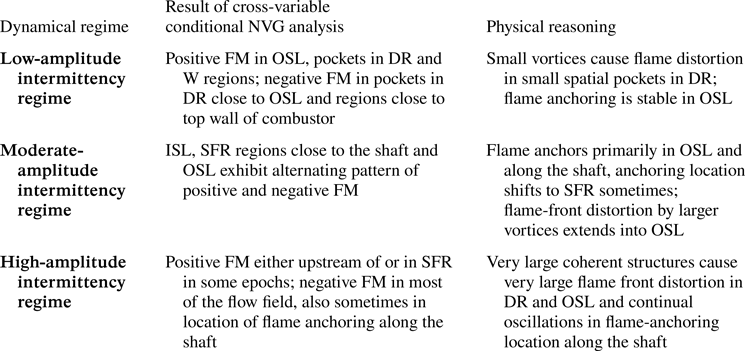
We discover that the frequency of local heat release rate fluctuations increases in regions of flame anchoring and decreases in regions associated with flame-front distortions, during bursts of high-amplitude  $p'$ dynamics. The spatial pattern of such cross-variable amplitude–frequency coupling varies across different dynamical regimes of intermittency obtained when the inlet airflow rate is varied continuously (summarised in table 3). As the mean flow velocity increases due to the continuous variation in the inlet airflow rate, the local flow time scale decreases, the mean acoustic pressure amplitude increases, epochs of periodicity in
 $p'$ increase and the mean size of coherent structures shed in the dump plane increases. As a result, the pattern of flow–flame–acoustic interactions vary and alter the flame-anchoring location and characteristics of flame-front distortion during low-, moderate- and high-amplitude intermittency dynamics. The understanding developed from such analysis can be useful in design and control of flame–acoustic interactions to increase operational margins of turbulent combustors. Further, the nature of flame–acoustic coupling can be investigated using this approach in other types of combustors with different flame-holding mechanisms, for premixed or partially premixed flames, and during different routes of transition to thermoacoustic instability such as a continuous or abrupt transition. An interesting pursuit for future works is to study the variations in the spatial pattern of FM during experiments involving continuous variation of the flow control parameter when the control parameter is varied at faster or slower rates.
Summary of results for different dynamical regimes obtained during the occurrence of intermittency prior to the onset of thermoacoustic instability when the air flow rate is varied continuously at a finite rate in experiments in a turbulent thermoacoustic system.

Funding
We acknowledge Dr V.R. Unni for fruitful discussions. This work was funded by the Office of Naval Research Global (ONRG) (grant number N629092212011). T.S. and R.R. acknowledge the support from Prime Minister Research Fellowship, Government of India.
Declaration of interests
The authors report no conflict of interest.
Data availability statement
The data that support the findings of this study are available from the corresponding author upon reasonable request.
Author contributions
S.T.: Writing (lead), analysis (equal), interpretation (lead), editing (equal), conceptualisation (equal); A.B.: Writing (equal), analysis (lead), interpretation (equal), editing (equal), conceptualisation (equal); R.R.: Experiments (lead), editing (equal); M.R.: Experiments (equal), editing (equal); G.C.: analysis (equal), interpretation (equal), editing (equal), conceptualisation (equal); R.I.S.: Editing (lead), analysis (equal), conceptualisation (equal), supervision (lead), funding (lead).
Appendix A. Effect of parameters used for short-window FFT to identify epochs of high- and low-amplitude dynamics in  $p'$

In this work, we investigate the frequency modulation (FM) in local heat release rate ( $\dot {q}'$) fluctuations associated with variations in the amplitude of acoustic pressure fluctuations (
 $p'$). Thus, we need to distinguish the epochs of high- and low-amplitude dynamics in
 $p'$. Towards this purpose, we use short-window fast Fourier transform computed over a window size
 $w$ corresponding to
 $L$ cycles of the dominant acoustic mode. Also, we place a threshold
 $A_\tau$ on the amplitude of the dominant frequency obtained across all windows as described in § 3.2. In the analysis presented in the main text, we use
 $L=5$ and
 $A_\tau =15\,\%$.
Here, we examine the effect of changes in the parameters  $L$ and
 $A_\tau$ used in the short-window FFT to identify epochs of high-amplitude
 $p'$ dynamics on the pattern of cross-variable amplitude–frequency coupling. From figure 9, we observe that on changing
 $A_\tau$, the threshold on the amplitude of dominant frequency obtained during short window FFT of
 $p'$, the spatial pattern of FM remains same qualitatively. However, the value and range of
 $K_{lh}$ changes slightly at each location.
The spatial pattern of  $K_{lh}$ obtained during the state of intermittency for quasi-static experiments when the short-window fast Fourier transform is computed for a window size
 $w$ corresponding to
 $L=5$ cycles of the dominant acoustic mode and the threshold on the amplitude of the dominant frequency is (
 $a$)
 $A_\tau =10\,\%$ and (
 $b$)
 $A_\tau =20\,\%$. The spatial pattern of FM in
 $\dot {q}'$ remains qualitatively the same for different
 $A_\tau$.

Further, if we change the window size for which the short-window FFT of  $p'$ is computed, we find again that the spatial pattern of FM is similar qualitatively (see figure 10). Positive FM appears in regions of flame anchoring, and negative FM occurs in regions of flame-front oscillations. Negative FM (blue regions) in the dump plane is more pronounced in figure 10(
 $a$) for shorter window sizes. Since the flame-anchoring conditions do not vary significantly for long epochs, we see that positive FM in the secondary flow regions is more pronounced for larger window sizes as evident in figure 10(
 $b$).
The spatial pattern of  $K_{lh}$ obtained during the state of intermittency for quasi-static experiments when the short-window fast Fourier transform is computed for a window size
 $w$ corresponding to (
 $a$)
 $L=4$ and (
 $b$)
 $L=7$ cycles of the dominant acoustic mode. In each case, the threshold on the amplitude of the dominant frequency is
 $A_\tau =15\,\%$. The spatial pattern of FM in
 $\dot {q}'$ remains qualitatively the same for different sizes of the window used for short-window FFT.

In summary, the results obtained for FM in local heat release rate fluctuations during high-amplitude  $p'$ dynamics are not very sensitive to changes in the parameters of the short-window FFT used to identify epochs of high- and low-amplitude
 $p'$ fluctuations.
Appendix B. Spatial variation of Rayleigh index during high- and low-amplitude $p'$ dynamics

The Rayleigh index ( $RI$) is calculated as given by (B1), where the integral over
 $t\in T$ represents conditional integration performed over all the epochs of high- (or low-) amplitude
 $p'$ dynamics identified by the method described in § 3.2. When
 $RI$ is calculated as a conditional average during the epochs of high-amplitude
 $p'$ dynamics, we denote it as
 $RI_h$, and similarly as
 $RI_l$ corresponding to low-amplitude
 $p'$ dynamics.
 \begin{equation} RI(x,y)=\frac{1}{|T|} \int_{t\in T} p'(t)\dot{q}'(x,y,t) \,{\rm d}t. \end{equation}
Here,  $|T|$ is the total length of the epochs of high- (or low-) amplitude
 $p'$ dynamics. In figures 11(
 $a$) and 11(
 $b$), we plot the spatial variation of the Rayleigh index
 $RI_h$ and
 $RI_l$ corresponding to high- and low-amplitude
 $p'$ dynamics, respectively.
Spatial variation of Rayleigh index  $RI$ plotted during epochs of (
 $a$) high-amplitude periodic and (
 $b$) low-amplitude aperiodic fluctuations in
 $p'$.

We find that  $RI_h$ is positive primarily in a spatial pocket in the outer shear layer region (OSL) upstream of the bluff-body and negative in parts of the inner shear layer (ISL) and wake region above the bluff-body (see figure 11
 $a$). Also,
 $RI_h$ is negative but close to zero in the secondary flow recirculation (SFR) region in figure 11(
 $a$). Further, during the epochs of low-amplitude fluctuations in
 $p'$, we find that the conditionally averaged Rayleigh index
 $RI_l$ is positive in the OSL, and in the wake region above and close to the bluff-body, but negative in the SFR and ISL regions upstream of the bluff-body (see figure 11
 $b$). Also, during low-amplitude fluctuations in
 $p'$, thermoacoustic power sources in OSL decrease.
Clearly, a coherent region of strong sources of thermoacoustic power (i.e. positive Rayleigh index) exist in the OSL during the epochs of high-amplitude oscillations in  $p'$. The spatial extent of these sources in the OSL decreases during epochs of low-amplitude
 $p'$ dynamics. We note that this spatial pocket is associated with the part of the flame that is anchored along OSL. Local mixing is enhanced in the OSL owing to fluid entrainment and strong recirculation created in the flow by the relatively larger vortices that are shed in the recirculation zone during the high-amplitude
 $p'$ dynamics. From our analysis presented in figure 6(
 $c$), we discover that the frequency of local
 $\dot {q}'$ dynamics increases in locations in the OSL where coherent thermoacoustic power sources occur during the epochs of high-amplitude
 $p'$ dynamics.
On comparing  $RI_h$ and
 $RI_l$ in SFR and ISL region adjacent to the bluff-body, we find that sinks of thermoacoustic power exist during both high- and low-amplitude
 $p'$ dynamics. However, the strength and spatial coherence of thermoacoustic power sinks increase during the epochs of low-amplitude
 $p'$ dynamics. These regions exhibit positive FM (evident in figure 6
 $c$).
Further, we find a coherent pocket of thermoacoustic power sinks during high-amplitude  $p'$ dynamics, and thermoacoustic power sources during low-amplitude
 $p'$ dynamics in a spatial pocket above and downstream of the bluff-body. Close to the top wall of the combustor, the large vortices impinge and undergo further combustion and the flame-front distortions are significant. Thus, we can infer that the heat release rate fluctuations in these regions are out of phase with
 $p'$ during high-amplitude oscillations, but become in phase with
 $p'$ during the low-amplitude fluctuations in
 $p'$. These regions exhibit negative FM in local
 $\dot {q}'$ dynamics as evident in figure 6(
 $c$).
In summary, we infer that regions where positive FM occurs, we find stronger sources or weaker sinks of thermoacoustic power during epochs of high-amplitude  $p'$ dynamics as compared with epochs of low-amplitude
 $p'$ dynamics.
Appendix C. Mean heat release rate dynamics during experiments with continuous variation in the airflow rate
Figure 12 shows the spatial pattern of mean heat release rate ( $\langle \dot {q}\rangle$) averaged over short time frames of
 $0.6$ s. The time frames indicated in figure 12 correspond to those in figure 8. The spatial pattern of average heat release rate indicates the flame dynamics during each epoch. We note that heat released is maximum in regions where the reactants and the hot products mix efficiently. Usually, these regions are associated with flame-front oscillations as the vortices containing the unburnt reactants distort the flame where hot products are contained after a combustion reaction. The flame anchoring and flame-front oscillations can hence be conjectured using heat release rate dynamics.
Spatial pattern mean heat release rate ( $\langle \dot {q}\rangle$) averaged over short time frames of
 $0.6$ s, corresponding to the plots of
 $K_{lh}$ shown in figure 8. The time frames I–XII in this figure correspond to the time frames shown in figure 8. The pattern of mean heat release rate delineate the flame dynamics during each short time frame.

For example, during time frames (I–IV) in figure 12(a), we see in experiments that the flame anchors predominantly close to the backward facing step and the flame front exists in the OSL and ISL. Thus, we find that an average maximum heat release rate occurs in the OSL in figure 12( $a$). These are the time frames we classified as low-amplitude intermittency regime.
Next, during the moderate-amplitude intermittency regime, corresponding to the time frames (V–VIII) shown in figure 12( $b$), we find that the flame anchors not only in the OSL close to the backward-facing step, but also in the ISL along the shaft upstream of the bluff-body. The flame front oscillates in the OSL, ISL and SFR regions, which are also the regions of maximum mean heat release rate in figure 12(
 $b$-V, VIII). Also, note that the flame-anchoring position can change along the shaft during some epochs. As a result, the flame can anchor in the SFR region and the flame front exists primarily in the ISL. Hence, we see that during certain time frames, the mean heat release rate is maximum only in the ISL and OSL, and not in the SFR region such as in figure 12(
 $b$-VI, VII).
Finally, during time frames (IX–XII) in figure 12( $c$) corresponding to high-amplitude intermittency regime, we find that the maximum of mean heat release rate oscillations occurs predominantly in the SFR and ISL regions. As noted earlier, the flame anchors along the shaft of the bluff-body and not in the OSL, and the flame anchors along the shaft at different locations during different epochs. In fact, the location of flame anchoring appears to oscillate to and fro along the shaft due to the periodic shedding of very large vortices in the dump plane. When the flame anchors upstream of the SFR region, then the SFR region is associated with flame-front oscillations. In contrast, when the flame anchors in the SFR region, the flame front exists primarily in the OSL and wake of the bluff-body.
As a result, we obtain high values of mean heat release rate in the SFR region as well as in the OSL, ISL and wake downstream of the bluff-body. The dynamic nature of flame anchoring can only be seen in experiments but cannot be seen in the mean heat release rate images. To characterise such dynamics, high-resolution Mie-scattering imaging is required which is a task for of future research.
Appendix D. Classification of the three dynamical regimes during the occurrence of intermittency in experiments with continuous variation in the airflow rate
To quantitatively distinguish the three intermittency regimes used in the main text, we consider variations in the root mean square of  $p'$ and
 $\dot {q}_G$ fluctuations. In figure 13, we plot the variation of
 $p'_{rms}$ and
 $\dot {q}_{G_{rms}}$ calculated for time windows
 $T_w=0.6$ s. We perform this analysis for the dynamics in
 $t \in [0,9.6]$ s corresponding to
 $16$ time windows as considered in the main text.
Variation of  $p'_{rms}$ and
 $\dot {q}_{G_{rms}}$ obtained for a time window of
 $T_w=0.6$ s during experiments in a turbulent bluff-body stabilised combustor, where the inlet airflow rate is varied continuously.

From figure 13, we observe that during the epoch corresponding to the first four time windows ( $t\in [0,2.4]$ s, regime I in figure 13), the mean amplitude of
 $p'$ and
 $\dot {q}_G$ fluctuations is very low and the values of
 $p'_{rms}$ and
 $\dot {q}_{G_{rms}}$ are also very low. We classify these four time windows as the low-amplitude intermittency regime. Next, during
 $t\in [2.4,4.8]$ s, we find that the value of
 $\dot {q}_{G_{rms}}$ increases notably while the value of
 $p'_{rms}$ is still low and the increase is small. This dynamical regime corresponds to the time windows 5–8 (regime II in figure 13) and are characterised by relatively longer bursts of periodicity in
 $p'$ as compared with that in regime I. We classify this regime as the moderate-amplitude intermittency regime.
Finally, during  $t\in [4.8,7.2]$ s (time windows 9–12, regime III in figure 13), we find that the values of both
 $p'_{rms}$ and
 $\dot {q}_{G_{rms}}$ increase significantly and continuously. Note that, the fluctuations in
 $p'$ exhibit intermittent bursts of periodicity amidst relatively low-amplitude aperiodic fluctuations during this epoch. We thus classify this regime of
 $t\in [4.8,7.2]$ s as the high-amplitude intermittency regime. For
 $t \in [7.8,9.6]$ s (regime IV in figure 13),
 $p'_{rms}$ and
 $\dot {q}_{G_{rms}}$ continue to increase; however,
 $p'$ exhibits limit cycle oscillations.
Appendix E. Effect of the length of time window $T_w$ used for analysis of intermittency during experiments with continuous variation of the airflow rate

For experiments with continuous variation of the flow parameter, we construct the visibility graph from local heat release rate signals for short time windows of  $T_w$ length. In § 4.2,
 $T_w=0.6$ s. The epochs of high- and low-amplitude
 $p'$ fluctuations are distinguished via short-window FFT performed over
 $L=5$ cycles of the dominant acoustic mode. To find the effect of the parameter
 $T_w$, we select three epochs of different
 $T_w$ with maximum overlap during the three different dynamical regimes of intermittency obtained during experiments with continuous variation of the flow parameter.
For example, during low-amplitude intermittency dynamics (row I in figure 14 $a$), we select three epochs and plot the spatial pattern of
 $K_{lh}$ during
 $t\in [1.225,1.775]$ s (
 $T_w=0.55$ s) in figure 14(
 $a$-I(A)),
 $t\in [1.2,1.8]$ s (
 $T_w=0.6$ s) in figure 14(
 $a$-I(B)) and
 $t\in [1.175,1.825]$ s (
 $T_w=0.65$ s) in figure 14(
 $a$-I(C)). Similarly, epochs of different lengths (
 $T_w=0.55, 0.6, 0.65$ s) but with maximum overlap are selected during moderate- and high-amplitude intermittency dynamics, and the spatial plots of
 $K_{lh}$ are shown in row II and row III in figure 14(
 $b$,
 $c$), respectively.
Spatial distribution of the ratio  $K_{lh}$ obtained during the state of intermittency observed in experiments with continuous variation of the inlet airflow rate during low-amplitude (row I), moderate (row II) and high-amplitude (row III) intermittency dynamics for different values of
 $T_w=0.55,0.6,0.65$ s in columns A, B, C, respectively. The epochs (
 $[t_1,t_2]$) selected are indicated in the title of each panel. We observe that the spatial pockets of positive and negative FM identified during different regimes are similar for different
 $T_w$.

Clearly, the spatial pockets of positive and negative FM identified during the epochs of different lengths ( $T_w$) are similar during all the three dynamical regimes of intermittency. Our inference of the physical processes involved in the flame–acoustic interactions are therefore not very sensitive to
 $T_w$. We also note that if we choose a very large time window for analysis, the variations of the mean amplitude of
 $p'$ within the time window will become significant. However, if a much smaller length of the time window is used for the analysis, the statistics of the network measures may not be reliable.