1. Introduction
In October 2008, the Federal Reserve began paying interest on both required and excess reserve balances. When the interest on reserves (IOR) rate exceeds the federal funds rate (FFR), banks face a reduced opportunity cost of holding reserves and may willingly accumulate large excess reserve balances rather than lend in the interbank market. Dutkowsky and VanHoose (Reference Dutkowsky and VanHoose2017) formalize this insight by showing that the introduction of IOR creates two distinct regimes: a scarce reserves regime, in which banks hold minimal excess reserves and actively lend in the wholesale market, and an abundant reserves regime, in which banks hold positive excess reserves and wholesale lending shuts down. By their estimates, banks operated predominantly in the abundant reserves regime from the end of 2008 through 2015. Williamson (Reference Williamson2012) shows theoretically that when reserves earn a return comparable to other short-term assets, open market operations (OMOs) become ineffective because reserves and bonds are perfect substitutes.
This shift in bank reserve management has important implications for the transmission of monetary policy. If banks are content holding large quantities of excess reserves, OMOs, traditionally the Fed’s primary tool for influencing economic conditions, may no longer transmit effectively to the broader economy. Carpenter and Demiralp (Reference Carpenter and Demiralp2012) provide early empirical evidence that the standard money multiplier mechanism does not describe the post-crisis relationship between reserves and broader monetary aggregates. I ask whether the introduction of IOR weakened the effectiveness of OMOs in influencing real output and the price level.
To answer this question, I estimate separate structural vector autoregression (SVAR) models for two sample periods using monthly U.S. data. The pre-IOR period spans 1967M1–2008M10, during which reserves earned no interest. The post-IOR period covers 2008M11–2018M10, during which the IOR rate was consistently above the FFR. I use the monetary base as the indicator of monetary policy and identify shocks through a combination of short- and long-run restrictions. This choice of policy indicator is motivated by Goodfriend (Reference Goodfriend2002) and Woodford (Reference Woodford2012), who argue that when the central bank pays interest on reserves, the quantity of reserves can move independently of the short-term interest rate, making the monetary base a highly informative indicator of OMO activity. The identification strategy, which builds on established frameworks in the SVAR literature, is detailed in Section 3.
The results indicate a clear structural break. In the pre-IOR period, a positive monetary base shock raises output to a peak of approximately 0.31% at month 10, with the 68% error band above zero from month 4 through the end of the horizon, after which the response decays toward the zero long-run value that the neutrality restriction imposes. The price level rises from the first month after the shock and remains permanently higher, reaching approximately 0.29% by the end of the 60-month horizon. In the post-IOR period, output responses are muted and statistically uncertain, and the price-level response is imprecisely estimated throughout. The money multiplier collapses over the same period, so base expansions were no longer amplified into broader money growth.
These findings contribute to two related literatures. First, a growing body of work has documented the microeconomic consequences of the IOR regime, including altered bank portfolios (Beckworth, Reference Beckworth2018; Ennis and Wolman, Reference Ennis and Wolman2015), depressed bank lending (Hogan, Reference Hogan2021), reduced daylight overdrafts (Hendrickson, Reference Hendrickson2017), and a muted reserves channel (Dave et al. Reference Dave, Dressler and Zhang2020). Theoretical work by Cochrane (Reference Cochrane2014) suggests that OMOs should be neutral when reserves pay competitive interest. My paper complements these studies by examining whether the aggregate macroeconomic effectiveness of OMOs, their impact on output and prices, was indeed diminished.
Second, this paper relates to the broader literature on monetary transmission mechanisms. Changes in the monetary base can affect the economy through several channels, including the portfolio balance, bank lending, and balance-sheet channels (Meltzer, Reference Meltzer1995; Mishkin, Reference Mishkin1995), each of which may operate differently when banks hold large excess reserves. My SVAR estimates the combined effect of monetary base shocks on output and prices, providing a macroeconomic assessment of whether OMOs retained their effectiveness after IOR. This approach complements studies of individual channels (Albertazzi et al. Reference Albertazzi, Becker and Boucinha2021; Lloyd, Reference Lloyd2017) and is consistent with the broad regime switches identified by Rich (Reference Rich2023). I combine short- and long-run restrictions so that I can impose monetary neutrality on the level of output and still identify the within-month timing that separates policy shocks from money demand shocks.
What I estimate here is the net effect of a monetary base expansion across all transmission channels operating at once. Studies of individual margins establish that bank behavior changed after 2008. They do not establish what those changes implied in aggregate, because channels may reinforce or offset one another, and the net effect is what monetary policy decisions depend on.
The result also matters for current policy. The ample-reserves framework, with IOR as the primary instrument, is no longer a crisis expedient but the Federal Reserve’s standing operating regime. If monetary base expansions have weaker effects on output and prices under that regime, then the historical evidence commonly invoked to justify balance-sheet policy, drawn largely from the pre-2008 environment, overstates what such policy can deliver. That matters for the scale of balance-sheet expansion required to achieve a given macroeconomic objective in a future downturn, and for whether balance-sheet tools are a substitute for, or only a complement to, conventional interest rate policy.
The rest of the paper is organized as follows. Section 2 provides background on the IOR policy, the monetary transmission mechanism, and the money multiplier. Section 3 describes the data and the SVAR identification strategy. Section 4 presents the empirical results. Section 5 provides concluding remarks.
2. IOR, reserve regimes, and monetary transmission
2.1. The IOR operating framework
Many economists have long advocated paying interest on bank reserves. Early proposals emphasized that reserve requirements impose an implicit tax on depository institutions because reserve balances historically earned no return. Paying interest on reserve balances reduces or eliminates this tax and can limit incentives for costly balance-sheet management aimed at minimizing reservable deposits. Tolley (Reference Tolley1957) and Friedman (Reference Friedman1960) made the case early, and Ireland (Reference Ireland2019) reviews it. In that sense, interest on reserves was initially viewed as a reform that would improve the efficiency of the banking system and the implementation of monetary policy.
The Federal Reserve obtained authority to pay interest on reserves in 2006, and implementation began in October 2008 during the financial crisis. Although it initially attracted less attention than large-scale asset purchases and emergency lending programs, IOR was a major shift in the operating environment for banks and short-term money markets (Dutkowsky and VanHoose, Reference Dutkowsky and VanHoose2017; Taylor, Reference Taylor2016). It is not a temporary crisis measure but a core component of the Federal Reserve’s operating framework (Woodford, Reference Woodford2012).
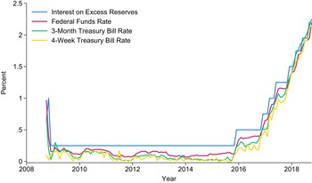
In principle, paying interest on reserves introduces an administered return that should place a floor under overnight lending rates. If a bank can earn the interest on reserves rate by holding balances at the Federal Reserve, it should be unwilling to lend reserves at a lower rate in private markets. In practice, however, key short-term rates traded below the interest on reserves rate for extended periods after 2008. Figure 1 shows that from November 2008 through October 2018, the interest on reserves rate often exceeded the FFR and short-maturity treasury bill rates.
Short-term interest rates 2008M10:2018M10.
Notes: This figure plots short-term interest rates from 2008M10 to 2018M10. The blue line represents the interest rate on excess reserves, the red line depicts the FFR, the green line is the three-month treasury bill rate, and the yellow line depicts the four-week treasury bill rate.
Source: Federal Reserve Bank of St. Louis’s Federal Reserve Economic Data (FRED).

A leading explanation is that some large lenders in overnight markets had limited access to earning interest on reserve balances. Government-Sponsored Enterprises (GSEs) and some other institutions were active lenders in the federal funds market but were not eligible to receive interest on reserve balances. As a result, these lenders were willing to lend at rates below the interest on reserves rate, while banks could profitably borrow at those rates and hold the proceeds as interest-earning reserve balances. This wedge weakened arbitrage and helps explain why the FFR and other short-term rates frequently remained below the interest on reserves rate over much of the post-2008 period.
To address this imperfect floor, the Federal Reserve introduced the Overnight Reverse Repurchase (ON RRP) facility in September 2013. The ON RRP facility extended access to a risk-free overnight rate to a broader set of counterparties, including money market funds and GSEs, that were not eligible to earn interest on reserve balances. By offering these institutions a rate at which they could place funds directly with the Federal Reserve, the ON RRP helped establish a more effective floor under short-term money market rates (Frost et al. Reference Frost, Logan, Martin, McCabe, Natalucci and Remache2015).Footnote 1
In light of these institutional changes, I ask whether monetary base expansions transmitted differently once the Federal Reserve began paying interest on reserve balances.
2.2. Transmission mechanisms
Mishkin (Reference Mishkin1995) and Meltzer (Reference Meltzer1995) survey several mechanisms through which monetary policy affects output and the price level. Four of them matter here, the interest rate channel, the portfolio balance channel, the bank lending channel, and the balance-sheet channel. The portfolio balance channel received considerable attention from policymakers during the crisis period, and then-Chairman Bernanke (Reference Bernanke2010) stated that the Federal Reserve’s asset purchases work “primarily through the so-called portfolio balance channel.” The observed effects of monetary policy reflect all of these mechanisms operating at once.
2.2.1. The interest rate channel
The interest rate channel is central in investment–saving and liquidity preference–money supply and New Keynesian frameworks. An expansionary policy lowers short-term nominal interest rates and, with sticky prices, reduces real borrowing costs, stimulating investment and consumption. After 2008, the Federal Reserve shifted toward administered rates. As Goodfriend (Reference Goodfriend2002) argues, IOR provides an additional instrument that can support the FFR, while OMOs manage reserve quantities. From this perspective, paying interest on reserves need not materially change transmission if policy can still move short-term rates in the desired direction.
2.2.2. The portfolio balance channel
Meltzer (Reference Meltzer1995) argues that focusing exclusively on interest rates is “overly restrictive” because monetary shocks also affect long-term rates, financial intermediation, and asset substitution. With imperfect asset substitution, open market purchases change relative asset supplies and induce portfolio reallocation, raising asset prices and easing financial conditions.Footnote 2 When reserves earn little or no return, banks have stronger incentives to rebalance into higher-yielding assets. When the IOR rate exceeds the FFR, however, banks tend to hold large reserve balances and interbank activity declines (Hendrickson, Reference Hendrickson2018), so portfolio reallocation may be weaker, and the effects of monetary base expansions may be muted.
2.2.3. The bank lending channel
The bank lending channel emphasizes that monetary policy can affect the economy by changing the supply of bank credit (Mishkin, Reference Mishkin1995). Before IOR, holding excess reserves earned no return, giving banks greater incentives to reallocate liquidity into loans. With IOR, banks may prefer to hold reserve balances rather than expand lending, weakening the lending response to a monetary base expansion. Hogan (Reference Hogan2021) finds that paying interest on excess reserves indeed reduced bank loan allocations.
2.2.4. The balance-sheet channel
The balance-sheet channel emphasizes the role of borrower net worth and the external finance premium (Bernanke et al. Reference Bernanke, Gertler and Gilchrist1999). Expansionary policy raises asset prices and collateral values, reducing agency costs and the external finance premium, a “financial accelerator.” If reserve remuneration increases the attractiveness of holding reserves relative to riskier assets, asset-price responses to monetary base expansions may be smaller and this amplification mechanism weaker.
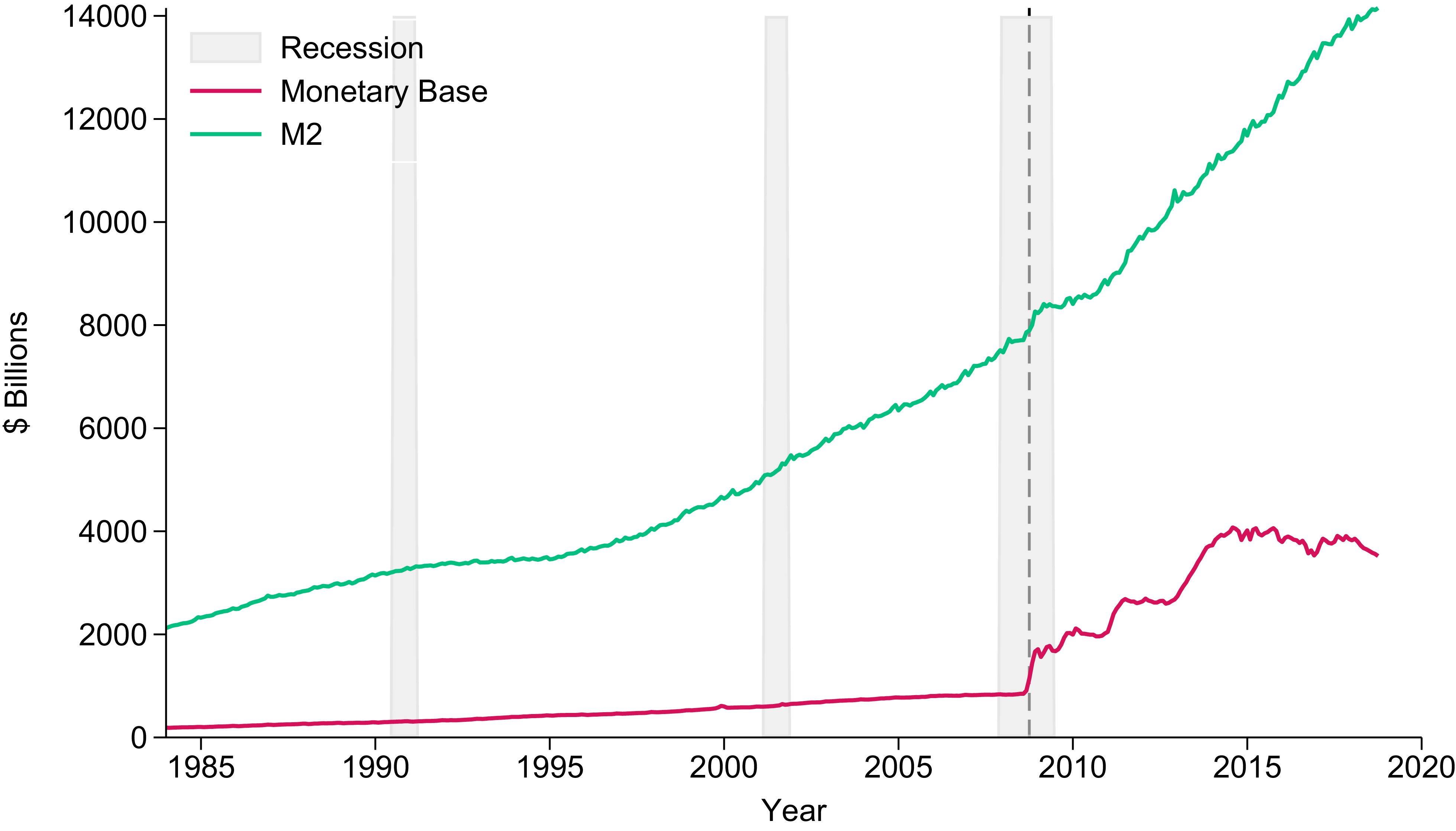
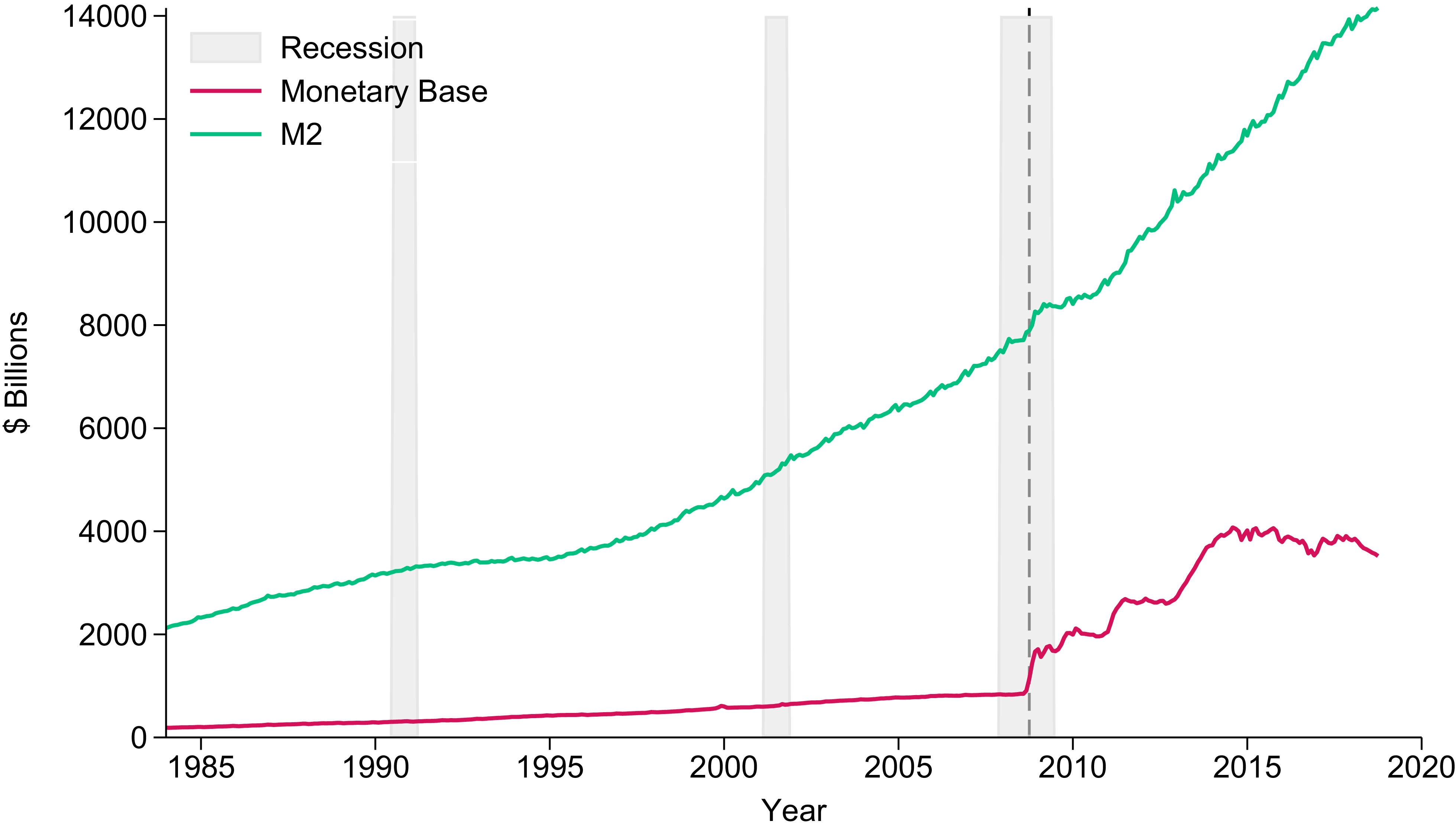
Money stock (M2) and monetary base, 1984M1–2018M10.
Notes: This figure plots broader monetary aggregate, M2, and the monetary base from 1984M1 to 2018M10. The green line represents M2, while the red line depicts the monetary base. The dashed line shows 2008M10, while the shaded bars indicate National Bureau of Economic Research (NBER) recession dates.
Source: Federal Reserve Bank of St. Louis’s Federal Reserve Economic Data (FRED).
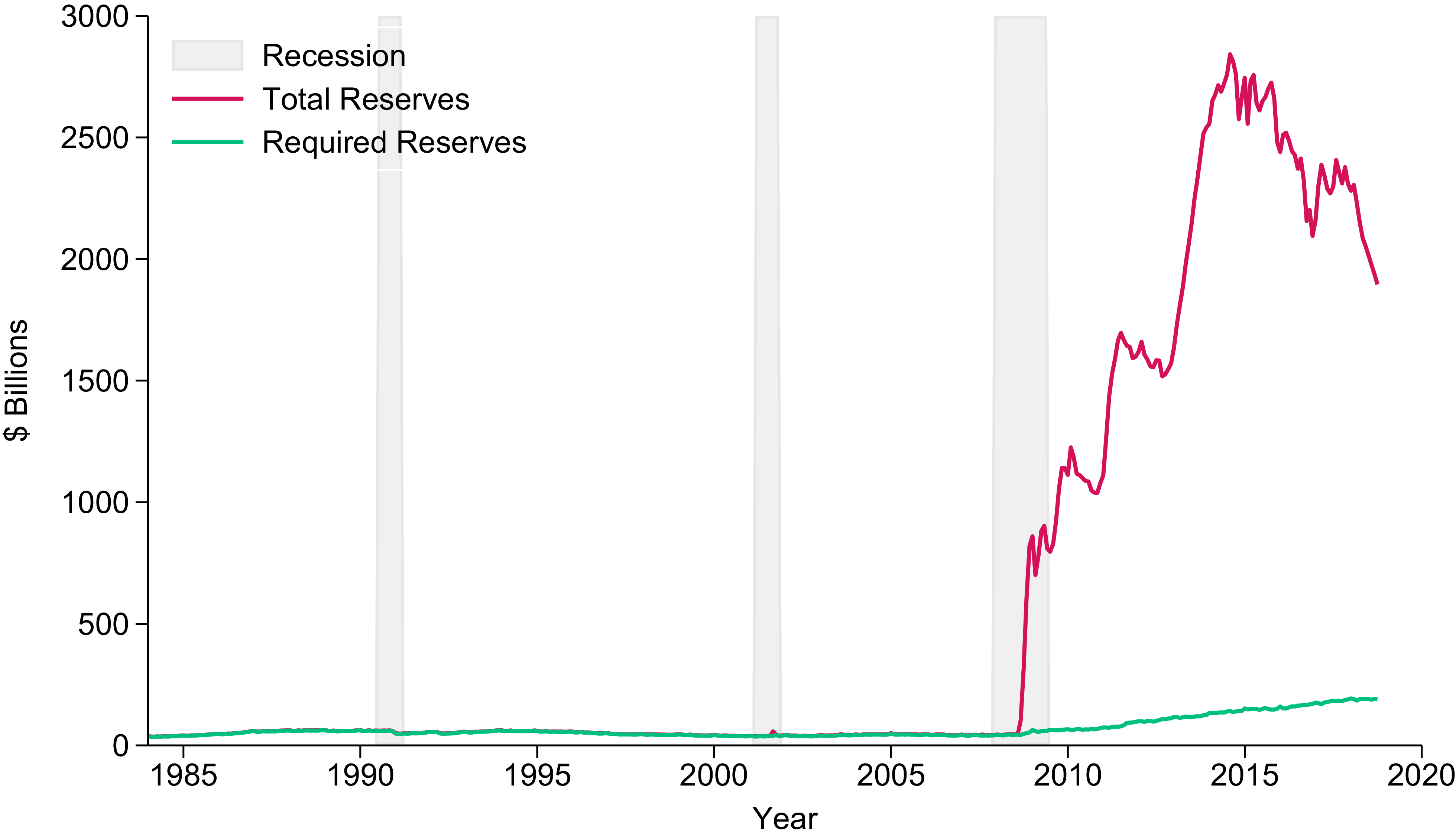
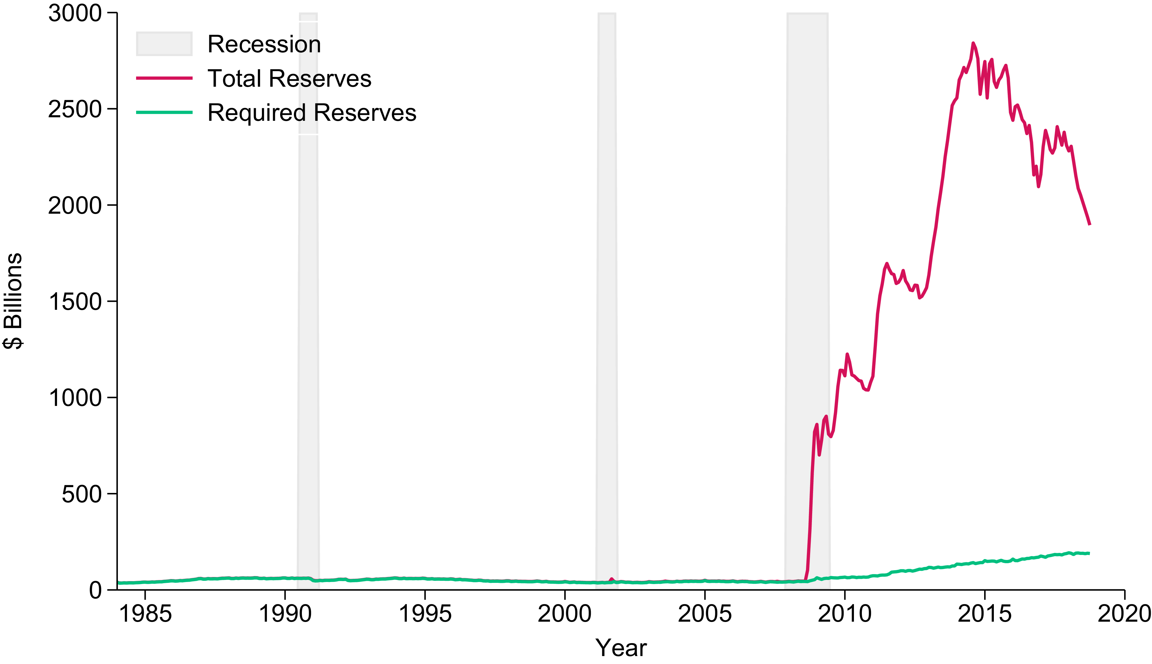
Total reserves and required reserves, 1984M1–2018M10.
Notes: This figure plots total against required reserves of depository institutions from 1984M1 to 2018M10. The red and green lines represent total reserves and required reserves, respectively, while the shaded bars indicate NBER recession dates.
Source: Federal Reserve Bank of St. Louis’s Federal Reserve Economic Data (FRED).
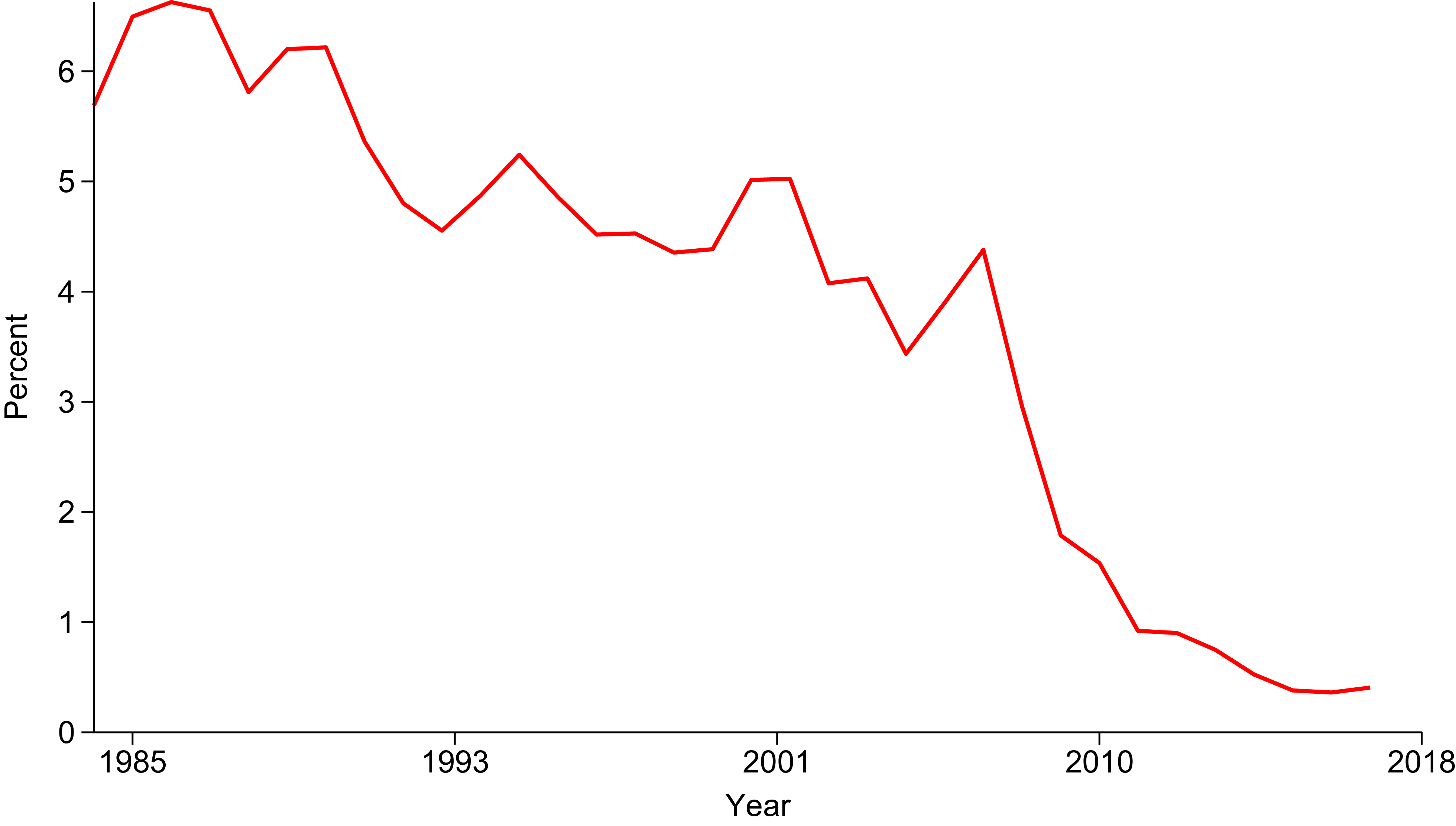
Year-end interbank lending as a percentage of total assets 1984–2017.
Notes: The red line in the figure represents the year-end interbank loans as a percentage of total assets from 1984 to 2017.
Source: Federal Reserve Bank of St. Louis’s Federal Reserve Economic Data (FRED).

2.3. Stylized facts: Reserves, multipliers, and interbank activity
A prominent expectation following the implementation of IOR was that banks would hold substantially more excess reserves, given the reduced opportunity cost. Despite the Fed’s extensive liquidity injections, the monetary base expansion did not translate into a corresponding increase in broader money measures (M2), indicating that banks were absorbing reserves rather than channeling them into the economy. Figure 2 illustrates this pattern. While the monetary base expanded rapidly after 2008, M2 grew at a much slower pace. Total reserves grew dramatically, and almost all of that growth was in excess reserves (Figure 3). Figure 4 shows that year-end interbank lending by U.S. commercial banks, as a percentage of total assets, fell from a range of 3–7% before 2008 to roughly 0.4% by 2017. This pattern is consistent with an operating environment in which large reserve balances and reserve remuneration reduce the role of interbank markets in reserve management.
Dutkowsky and VanHoose (Reference Dutkowsky and VanHoose2017) provide a theoretical framework for understanding this shift. In their model, the introduction of IOR creates the possibility of two distinct regimes.Footnote 3 Their quantitative analysis implies that from the end of 2008 through 2015, banks operated predominantly in the abundant reserves regime. They also show that banks can oscillate between regimes in response to changes in the relative levels of the FFR and IOR. Ennis and Wolman (Reference Ennis and Wolman2015) find similarly that banks shifted from holding minimal outside liquidity to holding substantially higher levels. Using Markov-switching Bayesian VARs, Rich (Reference Rich2023) identifies a switch in the Fed’s interest rate rule and in banks’ demand for outside money that coincides with the initiation of IOR.
The decline in the money multiplier provides further descriptive evidence of this structural shift. I measure the multiplier as the ratio of a broader monetary aggregate to the monetary base, and I report it under both Divisia and simple-sum aggregation. Divisia aggregates use index-number theory to weight components by their user costs, which gives a theoretically grounded measure of monetary services when the composition of liquid assets changes (Barnett, Reference Barnett1980; Diewert, Reference Diewert1976). Simple-sum aggregation weights every component equally. The Divisia M1 and M2 series used here are from the Center for Financial Stability.Footnote 4
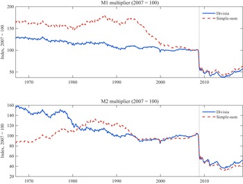
Figure 5 displays all four multipliers from January 1967 through October 2018. Before 2008 each is stable, with coefficients of variation of 1 to 3%. In 2008 each falls steeply and remains depressed, indicating a break in the relationship between the monetary base and broader measures of money. Once banks began earning interest on reserves at rates above the FFR, monetary base expansions were no longer amplified into proportional increases in broader money.
Divisia and simple-sum M1 and M2 money multipliers.
Notes: The figure plots money multipliers, defined as the ratio of a broader monetary aggregate to the monetary base, from 1967M1 to 2018M10. The top panel shows the M1 multiplier and the bottom panel the M2 multiplier. Solid blue lines are the Divisia multipliers, and dashed red lines are the corresponding simple-sum multipliers. Both series are indexed to 100 at their 2007 average so that the two aggregation methods can be compared on a common scale. The vertical dotted line marks the introduction of IOR in 2008M11.

The two aggregation methods diverge in earlier decades, so the choice is not innocuous in general, but they agree on the episode of interest. As of 2018, the Divisia M1 multiplier stands 45% below its 2007 level against 39% for simple-sum M1, and the Divisia M2 multiplier 50% below against 57% for simple-sum M2. The collapse comes principally from the denominator, since the monetary base roughly quadrupled over this period, so it does not depend on how the components of the numerator are weighted. I test in Section 4 whether the collapse in the multiplier is matched by weaker effects of monetary base shocks on output and the price level.
3. Empirical analysis
I test whether the introduction of IOR weakened the transmission of monetary base expansions to real output and the price level.
3.1. Data
The SVAR model describes the behavior of four variables: industrial production (IP), a personal consumption expenditures (PCE) chain-type price index, the FFR, and the monetary base.Footnote
5
IP represents real output,
 $Y_t$
, while PCE measures the price level,
 $P_t$
.Footnote
6
The FFR serves as the short-term nominal interest rate,
 $R_t$
, and the monetary base as the monetary aggregate,
 $M_t$
. Figure 6 plots the time series for these four variables over the full sample period.
U.S. macroeconomic data, 1967M1 - 2018M10.
Notes: The figure above plots the industrial production (Y), PCE price index (P), the effective federal funds rate (R), and the monetary base (M) from 1967M1 to 2018M10. All except R are first log-differenced and scaled by 100. The shaded bars indicate NBER recession dates.

The dataset consists of 622 monthly observations spanning January 1967 (1967M1) to October 2018 (2018M10). I split the data into two subsamples: the pre-IOR period (1967M1–2008M10), during which reserves earned no interest and the FFR exceeded any implicit return on reserves, and the post-IOR period (2008M11–2018M10), during which the IOR rate was consistently above the FFR. The pre-IOR sample contains 502 observations, and the post-IOR sample contains 120.
I end the post-IOR sample at 2018M10 so that the estimation window covers a single, stable IOR regime. After October 2018, the ordering of the IOR rate relative to the FFR became less stable, complicating the identification of the IOR regime.Footnote 7
IP, PCE, FFR, and monetary base are drawn from the Federal Reserve Bank of St. Louis’s Federal Reserve Economic Data (FRED) database. The Divisia monetary aggregates are from the Center for Financial Stability. The Divisia series enter only the money multiplier comparison in Section 2.3. The SVAR uses the monetary base, which is not aggregation-weighted, so the impulse responses and variance decompositions do not depend on the choice between Divisia and simple-sum aggregation. For both periods, the Augmented Dickey-Fuller and the Phillips-Perron unit root tests indicate that all variables, except for the FFR, are non-stationary in their level form.Footnote 8 To induce stationarity, all variables enter the model in first log differences, except for the FFR, which enters in levels (percentages).
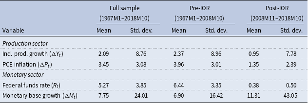
Table 1 presents summary statistics for the full sample and for the pre- and post-IOR subperiods. The monetary environment differs substantially across the two regimes. In the pre-IOR period, annualized monetary base growth is relatively stable, with a standard deviation of 16.42%. In the post-IOR period, this volatility rises to 43.05%, consistent with the large expansion and fluctuations in reserve balances associated with large-scale asset purchases. Over the same period, the standard deviation of PCE inflation falls from 3.01% to 2.39%, and the volatility of IP growth also declines. These unconditional moments suggest that the post-2008 period featured a much more volatile monetary base alongside less volatile inflation and output growth, a pattern consistent with a weakened transmission mechanism and motivating the formal SVAR analysis below.
Summary statistics

Table 1. Long description
A table comparing summary statistics for the full sample and for the pre- and post-IOR subperiods. The table has four rows and six columns. The columns are labeled as Full sample (1967M1-2018M10), Pre-IOR (1967M1-2008M10), and Post-IOR (2008M11-2018M10), each with Mean and Std. dev. The rows are labeled as Production sector and Monetary sector. Row 1: Ind. prod. growth (ΔYt), 2.09, 8.76, 2.37, 8.96, 0.95, 7.78. Row 2: PCE inflation (ΔPt), 3.45, 3.08, 3.96, 3.01, 1.35, 2.39. Row 3: Federal funds rate (Rt), 5.27, 3.85, 6.44, 3.35, 0.38, 0.50. Row 4: Monetary base growth (ΔMt), 7.75, 24.01, 6.90, 16.42, 11.31, 43.05. The table reports annualized means and standard deviations. The federal funds rate is expressed in percent. For industrial production, inflation, and the monetary base, the monthly log-difference growth rates are multiplied by 1,200 to present them in annualized percentage terms.
Notes: The table reports annualized means and standard deviations. The federal funds rate is expressed in percent. For industrial production,inflation, and the monetary base, the monthly log-difference growth rates are multiplied by 1,200 to present them in annualized percentage terms.
3.2. Methods
The principal objective is to estimate the impulse responses of output and the price level to a monetary policy shock, both inside and outside of periods where the interest rate on reserves exceeds the FFR.
Collecting the variables into the
 $4 \times 1$
vector,
 \begin{equation*} Z_t = [\begin{array}{c} Y_t \quad P_t \quad R_t \quad M_t \end{array}]', \end{equation*}
the structural model takes the form
 \begin{equation} AZ_t = \Phi _1 Z_{t-1} + \ldots + \Phi _j Z_{t-j} + \varepsilon _t, \quad \varepsilon _t \sim N(0_{4\times 1}, I_4) \end{equation}
where
 $A$
is an invertible
 $4 \times 4$
matrix of contemporaneous structural coefficients,
 $\Phi _1, \ldots , \Phi _j$
are
 $4 \times 4$
autoregressive coefficient matrices, and
 $\varepsilon _t$
is a
 $4 \times 1$
vector of serially and mutually uncorrelated structural disturbances.Footnote
9
The model is estimated with 5 lags for the pre-IOR sample and 3 lags for the post-IOR sample. Information criteria select three lags for the post-IOR sample. For the pre-IOR sample, the Akaike criterion (Akaike, Reference Akaike1974) is nearly flat between four and six lags, and I use five.
I obtain the reduced form by premultiplying (3.1) by
 $A^{-1}$
:
 \begin{equation} Z_t = \Gamma _1 Z_{t-1} + \ldots + \Gamma _j Z_{t-j} + u_t, \end{equation}
where
 $\Gamma _j = A^{-1}\Phi _j$
, the reduced-form residuals are
 $u_t = A^{-1}\varepsilon _t$
, and
 \begin{equation} E[u_t u_t'] = \Omega = A^{-1}(A^{-1})'. \end{equation}
The reduced-form vector autoregression (VAR) can be expressed in moving-average form using lag operators:
 \begin{equation} Z_t = C(L) u_t, \end{equation}
where
 $C(0) = I_4$
and
 $C(1)$
captures the cumulative long-run effect of a reduced-form innovation. Substituting
 $u_t = A^{-1}\varepsilon _t$
gives the structural moving-average representation
 $Z_t = D(L)\varepsilon _t$
with
 $D(L) = C(L)A^{-1}$
, whose coefficient matrices are the dynamic multipliers of the structural innovations.
 $D(0) = A^{-1}$
is the matrix of impact responses and
 $D(1)$
the matrix of cumulative long-run responses. I impose the identifying restrictions on these two matrices. In both, rows index the variables of
 $Z_t$
and columns index the structural shocks.
3.2.1. Identification
The identification scheme imposes a combination of short- and long-run restrictions to recover four structural shocks: an aggregate supply shock, an aggregate demand shock, a money demand shock, and a monetary policy shock. I focus on the monetary policy shock, which corresponds to an exogenous expansion of the monetary base, that is, an OMO. This quantity-based identification is appropriate because the research question concerns the transmission of monetary base expansions, and in the IOR environment the monetary base can move independently of the short-term interest rate (Goodfriend, Reference Goodfriend2002; Woodford, Reference Woodford2012).
The short-run restrictions reflect informational and institutional frictions that govern within-period timing. Production and pricing decisions are governed by contracts and pre-planned schedules and do not adjust instantaneously to monetary shocks (Leeper and Zha, Reference Leeper and Zha2003). Symmetrically, the Fed cannot observe production-sector variables within the month and infers conditions from the money stock and interest rate (Gordon and Leeper, Reference Gordon and Leeper1994). These assumptions yield four zero restrictions on the impact matrix
 $D(0)$
.
The long-run restrictions impose theoretical properties of the model’s steady state. Following Blanchard and Quah (Reference Blanchard and Quah1989), aggregate demand shocks have no permanent effect on the level of real output. Following Beckworth and Hendrickson (Reference Beckworth and Hendrickson2012), monetary policy shocks are neutral in the long run and cannot permanently alter real output. These two restrictions on the cumulative response matrix
 $D(1)$
are standard in the literature and are testable implications of a broad class of macroeconomic models.
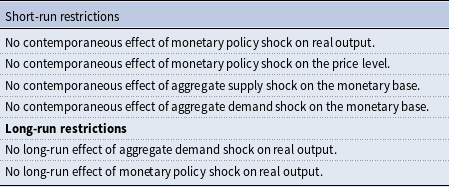
Together, the four short-run and two long-run restrictions provide exactly the six restrictions needed to identify the four-variable SVAR. This combination of short- and long-run restrictions follows Galí (Reference Galí1992), who was among the first to use both types in an SVAR to study the effects of money supply shocks, and Cecchetti and Rich (Reference Cecchetti and Rich2001), who employ a similar scheme to estimate the sacrifice ratio. Table 2 summarizes the restrictions. Appendix B verifies that the model satisfies the rank conditions for global identification established by Rubio-Ramirez et al. (Reference Rubio-Ramirez, Waggoner and Zha2010).
Summary of identifying restrictions
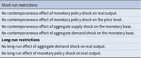
Table 2. Long description
A table summarizing identifying restrictions for a four-variable structural vector autoregression (SVAR) model. The table has two main sections: Short-run restrictions and Long-run restrictions. Short-run restrictions: No contemporaneous effect of monetary policy shock on real output. No contemporaneous effect of monetary policy shock on the price level. No contemporaneous effect of aggregate supply shock on the monetary base. No contemporaneous effect of aggregate demand shock on the monetary base. Long-run restrictions: No long-run effect of aggregate demand shock on real output. No long-run effect of monetary policy shock on real output.
3.2.2. Short-run restrictions
The model parameterizes the impact matrix
 $D(0) = A^{-1}$
as
 \begin{equation} \begin{array}{cc} & \begin{array}{c@{\qquad }c@{\qquad }c@{\qquad}c} \varepsilon ^{as}_t & \varepsilon ^{ad}_t & \varepsilon ^{md}_t & \varepsilon ^{mp}_t \end{array}\\ \begin{array}{c} Y_t \\ P_t \\ R_t \\ M_t \end{array}& \left [\begin{array}{c@{\quad }c@{\quad }c@{\quad }c} d_{11}(0) & d_{12}(0) & d_{13}(0) & 0 \\ d_{21}(0) & d_{22}(0) & d_{23}(0) & 0 \\ d_{31}(0) & d_{32}(0) & d_{33}(0) & d_{34}(0) \\ 0 & 0 & d_{43}(0) & d_{44}(0) \end{array}\right ] \end{array}. \end{equation}
I partition
 $Z_t$
into two sectors. Real output and the price level constitute the production sector, representing the objectives of monetary policy. The interest rate and the monetary base form the monetary sector.
The first set of identifying assumptions is that monetary policy shocks (positive innovations in the monetary base) affect the production sector only with a lag. Following Leeper and Zha (Reference Leeper and Zha2003), this inertia arises because pricing and production decisions are governed by contracts and pre-planned schedules that do not adjust instantaneously to money market conditions:
 \begin{equation*} \text{SR1}: \, d_{14}(0) = d_{24}(0) = 0. \end{equation*}
In the monetary sector, I leave the third row of
 $D(0)$
unrestricted, so the FFR responds within the month to all four shocks. Money supply and money demand are then jointly determined within the period, which Leeper and Zha (Reference Leeper and Zha2003) treat as essential for capturing the interaction between the monetary base and the FFR. Leaving this row free also allows the interest rate to move contemporaneously with output, the price level, and the monetary base, as a money demand schedule with the usual scale and opportunity cost arguments would require.
In the fourth row, I set the impact responses of the monetary base to the aggregate supply and aggregate demand shocks to zero. Following Gordon and Leeper (Reference Gordon and Leeper1994), within the month the Fed does not directly observe production-sector variables but infers economic conditions by monitoring the money stock and the interest rate, so the base cannot respond within the month to disturbances originating in the production sector. I identify monetary policy shocks through the contemporaneous interaction between the monetary base and the interest rate, and Sims and Zha (Reference Sims and Zha2006) and Belongia and Ireland (Reference Belongia and Ireland2015) adopt a policy rule with the same information structure. This yields the second set of short-run restrictions:
 \begin{equation*} \text{SR2}: \, d_{41}(0) = d_{42}(0) = 0. \end{equation*}
3.2.3. Long-run restrictions
I impose the long-run identification by restricting the elements of the cumulative response matrix
 $D(1)$
, which follows the same row and column convention as equation (3.5):
 \begin{equation} \begin{array}{cc} & \begin{array}{c@{\qquad }c@{\qquad }c@{\qquad }c} \varepsilon ^{as}_t & \varepsilon ^{ad}_t & \varepsilon ^{md}_t & \varepsilon ^{mp}_t\\ \end{array}\\ \begin{array}{c} Y_t \\ P_t \\ R_t \\ M_t \\ \end{array}& \left [\begin{array}{c@{\quad }c@{\quad }c@{\quad }c} d_{11}(1) & 0 & d_{13}(1) & 0 \\ d_{21}(1) & d_{22}(1) & d_{23}(1) & d_{24}(1) \\ d_{31}(1) & d_{32}(1) & d_{33}(1) & d_{34}(1) \\ d_{41}(1) & d_{42}(1) & d_{43}(1) & d_{44}(1) \\ \end{array}\right ]\\ \end{array}. \end{equation}
The first long-run restriction follows Blanchard and Quah (Reference Blanchard and Quah1989). The identifying assumption is that aggregate demand shocks have no permanent effect on the level of real output. This restriction helps distinguish between supply and demand shocks:
 \begin{equation*} \text{LR1}: \, d_{12}(1) = 0. \end{equation*}
The second long-run restriction imposes monetary neutrality, as in Beckworth and Hendrickson (Reference Beckworth and Hendrickson2012). Monetary policy shocks have no permanent effect on real output:
 \begin{equation*} \text{LR2}: \, d_{14}(1) = 0. \end{equation*}
To assess the reliability of the estimated impulse responses, I construct error bands from 10,000 Monte Carlo replications.
4. Results
Subsection 4.1 compares the impulse responses to a monetary policy shock across the two regimes. Subsection 4.2 turns to the forecast error variance decompositions (FEVDs), which show the same break in the composition of monetary base variation. I report impulse responses and variance decompositions for the remaining identified shocks in Appendix A.
4.1. Impulse response functions
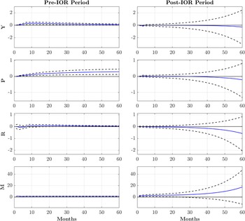
Figure 7 displays cumulative impulse-response functions for each variable to a one-standard-deviation positive monetary policy shock in both the pre-IOR and post-IOR periods. I sum the responses of output, the price level, and the monetary base, which enter the model in log differences, so the figure shows the cumulative effect on their log levels. The FFR enters in levels and is not accumulated. The solid line plots the mean response and the dashed lines correspond to 68% error bands constructed from 10,000 Monte Carlo replications.
Impulse response functions to identified monetary policy shocks.
Notes: IRFs to a one-standard-deviation shock to monetary policy (M). In each graph, the solid blue line represents the mean estimate, while the two dashed lines represent 68% error bands.

In the pre-IOR period, the monetary policy shock produces responses consistent with standard macroeconomic theory. Restriction SR1 holds real output at zero on impact, after which output rises to a peak cumulative response of approximately 0.31% at month 10 and then decays slowly. The 68% error band lies above zero from month 4 through the end of the horizon, so the output effect is well determined at 57 of the 60 horizons. Zero falls inside the band only over the first three months, while the cumulative response is still building. Restriction LR2 requires the response to return to zero eventually, and by month 60 it has fallen to about a third of its peak.
The price level is likewise zero on impact and then rises steadily, remaining permanently higher, with a cumulative response of approximately 0.29% by month 60. The 68% error band lies above zero from month 2 onward, so the price-level effect is precisely estimated and persistent. The FFR exhibits a brief liquidity effect, declining to approximately 6 basis points below zero within the first three months, before rising to approximately 8 basis points by month 15 and then gradually returning toward zero. The monetary base shows a persistent increase, consistent with the shock being identified as an exogenous expansion in the supply of reserves.
These responses are consistent with a functioning transmission mechanism in which monetary base expansions are intermediated through the banking system into broader money growth and, ultimately, into higher output and prices.
In the post-IOR period, the same monetary policy shock produces very different responses. The mean output response stays close to zero at every horizon, and its 68% error band contains zero from month 4 onward, dipping slightly below zero only at months 2 and 3. The price level is zero on impact, as before, and its error band contains zero at every subsequent horizon, so the post-IOR price effect is imprecisely estimated throughout. The FFR and monetary base responses are likewise imprecise, with error bands encompassing zero at most horizons.
The post-IOR error bands widen with the forecast horizon and, beyond about two years, are considerably wider than their pre-IOR counterparts. That widening comes from the accumulation of forecast uncertainty in a sample whose estimated dynamics lie closer to a unit root. Identification is unaffected. At the horizons where the pre-IOR effect peaks, around ten to twelve months, the two sets of bands are of comparable width.
These results are consistent with the theoretical framework outlined in Section 2.2. When the IOR rate exceeds the FFR, banks face a reduced incentive to rebalance away from reserves into loans or other assets, dampening the channels through which monetary base expansions traditionally affect the broader economy. These results are consistent with a weakening of the aggregate transmission of OMOs following the introduction of IOR.
The money multiplier evidence in Section 2.3 provides complementary support. As shown in Figure 5, Divisia money multipliers were relatively stable before 2008 and collapsed thereafter, indicating that expansions in the monetary base were no longer amplified into proportional increases in broader monetary aggregates.
Because the SVAR captures the aggregate effect of monetary base shocks, the muted post-IOR responses reflect the combined response across all operative transmission channels, including the bank lending, portfolio balance, and balance-sheet channels discussed in Section 2.2.
The parameters themselves changed across the two periods. A likelihood-ratio test of parameter constancy at 2008M11, computed on the pooled 1967M1–2018M10 sample so that the unequal subsample lengths play no role in it, rejects decisively, with
 $LR = 883.2$
and 52 degrees of freedom (
 $p \lt 10^{-128}$
) at three lags and
 $LR = 946.6$
with 84 degrees of freedom at five. Rescaling both regimes to a shock that raises the monetary base by 1% on impact, the post-IOR output response is
 $0.00$
with a 68% band of
 $[\!-0.11, 0.10]$
, against
 $0.29$
with a band of
 $[0.11, 0.49]$
before IOR. The post-IOR band is the narrower of the two, so the muted response is precisely estimated and indistinguishable from zero. I set out the rescaling, the equal-length windows, and the crisis-excluded specifications in Appendix C.1.
4.2. Forecast error variance decompositions
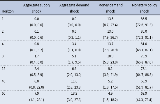
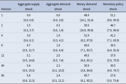
To complement the impulse-response analysis, I examine how the composition of monetary base variability changed across regimes. Tables 3 and 4 report FEVDs of the monetary base for the pre- and post-IOR periods up to a 60-month horizon. Because the FEVDs are highly asymmetrical from the Monte Carlo integration process, I report medians rather than means, so the center estimates do not sum to 100% at most horizons. One-standard-deviation error bands are reported in parentheses.Footnote 10
Pre-IOR—variance decomposition of monetary base,
 $M$
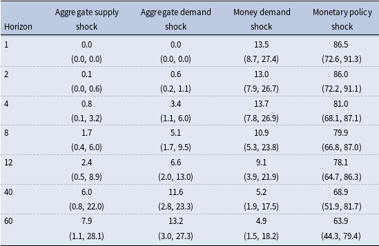
Table 3. Long description
A table titled ‘Pre-IOR variance decomposition of monetary base’ presents the decomposition of monetary base variability across different shocks and horizons. The table has 8 rows and 5 columns. The columns are labeled ‘Horizon’, ‘Aggregate supply shock’, ‘Aggregate demand shock’, ‘Money demand shock’, and ‘Monetary policy shock’. Each row corresponds to a specific horizon ranging from 1 to 60 months. The values in the table represent the median variance decomposition percentages, with one-standard-deviation error bands reported in parentheses. For example, at horizon 1, the values are 0.0 for aggregate supply shock, 0.0 for aggregate demand shock, 13.5 for money demand shock, and 86.5 for monetary policy shock, with error bands (0.0, 0.0), (0.0, 0.0), (8.7, 27.4), and (72.6, 91.3) respectively. The table shows how the composition of monetary base variability changes across different horizons and types of shocks.
Post-IOR—variance decomposition of monetary base,
 $M$
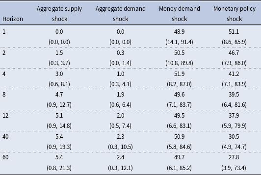
Table 4. Long description
A table comparing the variance decomposition of the monetary base post-IOR across different shocks and horizons. The table has 7 rows and 5 columns. Column headers are Horizon, Aggregate supply shock, Aggregate demand shock, Money demand shock, and Monetary policy shock. Row labels are 1, 2, 4, 8, 12, 40, and 60. Row 1: Horizon, 1, Aggregate supply shock, 0.0, Aggregate demand shock, 0.0, Money demand shock, 48.9, Monetary policy shock, 51.1. Row 2: Horizon, 2, Aggregate supply shock, 1.5, Aggregate demand shock, 0.3, Money demand shock, 50.5, Monetary policy shock, 46.7. Row 3: Horizon, 4, Aggregate supply shock, 3.0, Aggregate demand shock, 1.0, Money demand shock, 51.9, Monetary policy shock, 41.2. Row 4: Horizon, 8, Aggregate supply shock, 4.7, Aggregate demand shock, 1.9, Money demand shock, 49.6, Monetary policy shock, 39.5. Row 5: Horizon, 12, Aggregate supply shock, 5.1, Aggregate demand shock, 2.0, Money demand shock, 49.5, Monetary policy shock, 37.9. Row 6: Horizon, 40, Aggregate supply shock, 5.4, Aggregate demand shock, 2.3, Money demand shock, 50.9, Monetary policy shock, 30.5. Row 7: Horizon, 60, Aggregate supply shock, 5.4, Aggregate demand shock, 2.4, Money demand shock, 49.7, Monetary policy shock, 27.8.
In the pre-IOR period, monetary policy shocks account for the vast majority of base variation, 86.5% on impact, declining to 63.9% at the 60-month horizon (Table 3). Money demand shocks explain a modest 13.5% on impact. This pattern indicates that movements in the monetary base during this period were overwhelmingly driven by exogenous policy actions, namely, OMOs.
In the post-IOR period, this composition changes (Table 4). Money demand shocks account for 48.9% of base variation on impact, up from 13.5% before IOR, while the monetary policy share falls from 86.5 to 51.1%. The shift widens with the horizon. At 60 months, money demand accounts for 49.7% against 27.8% for monetary policy, which reverses the pre-IOR ordering. The post-IOR shares are estimated imprecisely, as is characteristic of variance decompositions computed on 120 observations, so I treat the comparison as descriptive. This shift is consistent with the post-IOR operating framework. Before 2008, the Fed influenced short-term rates primarily through OMOs that changed the supply of reserves, so shocks originating in the policy equation dominated base variation. After 2008, the Fed sets the IOR rate administratively, and the FFR adjusts to this administered rate rather than to reserve quantities. Shocks originating in the interest rate equation now account for the larger share of base variation, so the interest rate has become the primary driver of monetary base dynamics.
This change in composition accords with the impulse-response evidence that the nature of monetary base movements changed after the introduction of IOR. In the pre-IOR environment, the base moved primarily because the Fed pushed reserves into the system through OMOs. In the post-IOR environment, base movements are increasingly driven by the interest rate equation, consistent with a framework in which the administratively set IOR rate drives the FFR, which in turn influences reserve dynamics. This distinction helps explain the muted impulse responses documented in Subsection 4.1: if a smaller share of base movements represents exogenous policy, it follows that monetary base shocks would have diminished macroeconomic effects.
The main findings hold under alternative specifications, reported in Appendix C. That appendix takes up the two identification concerns raised by the short post-IOR sample and the coincidence of IOR with the financial crisis, re-estimating the model on equal-length pre-IOR windows, on a sample that excludes the crisis, with financial-stress controls in both regimes, on a sample extended through 2025M12, and with the IOR-FFR spread in place of the FFR. In every case the output and price-level responses to monetary base shocks remain muted after IOR.
5. Conclusion
This paper examines whether the introduction of interest on reserves in October 2008 weakened the aggregate transmission of OMOs to real output and the price level. Using an SVAR with short- and long-run restrictions estimated on monthly data from 1967M1 to 2018M10, I compare impulse responses to a monetary base shock across the pre-IOR period (1967M1–2008M10) and the post-IOR period (2008M11–2018M10).
The results indicate a clear change in the effectiveness of monetary base expansions. In the pre-IOR period, a positive monetary base shock raises real output over nearly the whole five-year horizon and moves the price level onto a permanently higher path. After IOR, the responses to the same shock are muted and imprecisely estimated. The share of monetary base variability due to monetary policy shocks roughly halves across the two regimes, and money demand shocks take the larger share at longer horizons. This shift is consistent with an environment in which the primary driver of monetary base dynamics is the interest rate, set administratively through the IOR rate, rather than reserve supply.
These findings have implications for the conduct of monetary policy. In an environment where reserves earn a rate above the FFR, expanding the monetary base through OMOs may not transmit to the broader economy as effectively as it did before 2008. This does not imply that monetary policy is ineffective, since the Fed retains influence through its administered rates, forward guidance, and other tools. It does suggest that the quantity-based channel of transmission has been weakened. Policymakers relying on balance-sheet expansion as a stimulus tool should account for the dampening effect of IOR on the intermediation of reserves into broader monetary aggregates.
The Federal Reserve began paying interest on reserves three weeks after the Lehman failure, so I cannot fully separate the policy from the crisis. The responses remain muted once the acute crisis is excluded, once financial-stress controls enter both regimes, and once the sample runs through 2025M12. The evidence is therefore consistent with the IOR regime, and it does not establish that IOR alone caused the change.
Microdata on bank lending, portfolio composition, or interbank market activity would help disentangle which transmission channels IOR affects most. Extending the analysis to other central banks that have adopted interest on reserves, such as the European Central Bank, the Bank of England, and the Bank of Japan, would show whether the dampening documented here is a general feature of floor systems or specific to the U.S. institutional environment.
Acknowledgements
I thank the editor, William A. Barnett, the associate editor, and two anonymous referees for their helpful comments, which substantially improved the paper. I am grateful to my graduate advisor, Joshua Hendrickson, for his guidance and support, and to my dissertation committee members, Kenneth Rich, John Conlon, and Kathleen Fuller, for their suggestions. I also thank Peter Ireland, Ron Mau, Andrew Hanson, Kwabena Boateng, and seminar participants at the University of Mississippi for valuable discussions. All remaining errors are my own.
Competing interests
The author declares none.
Appendix
A. Additional results
In this section I report the impulse responses to the remaining identified shocks and the forecast error variance decompositions (FEVDs) for both periods.
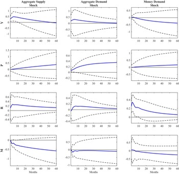
In Figure A.1, I present the impulse-response functions (IRFs) for all variables to one-standard-deviation shocks to aggregate supply, aggregate demand, and money demand in the pre-IOR period. As with the main results, the blue solid line represents the mean response, while the black dashed lines represent 68% error bands. In response to a positive innovation in output, the price level starts to rise slowly after the shock, indicating a delayed pass-through of supply-side changes to consumer prices. The federal funds rate increases, while the monetary base contracts, following a shock to aggregate supply. This is potentially a monetary policy response to prevent inflation from escalating. In the second column, I plot the IRFs to a one-standard-deviation aggregate demand shock. Following an exogenous increase in the price level, output rises on impact and returns to its initial level, as restriction LR1 imposes. It also leads to a permanently higher price level. Finally, the positive innovation in the price level generates a short-term liquidity puzzle. The FFR falls on impact, and the monetary base, which restriction SR2 holds at zero on impact, falls over the months that follow. Thereafter, the FFR rises while the monetary base continues to fall, consistent with policy tightening to keep inflation under control. The third and final column of Figure A.1 plots the IRFs to a one-standard-deviation increase in money demand. The money demand shock leads to a permanently lower output level. The price level does not move on impact and rises only after several months. I also observe a short-run liquidity puzzle, as the monetary base initially rises alongside the federal funds rate. Most of these responses are uncertain, with zero lying within the 68% error bands.
Pre-IOR: IRFs to identified shocks.
Notes: Cumulative IRFs to one-standard-deviation aggregate supply, aggregate demand, and money demand shocks, estimated on 1967M2–2008M10 with five lags. In each panel, the solid blue line is the mean response and the two dashed lines are 68% error bands. Vertical scales differ across panels.

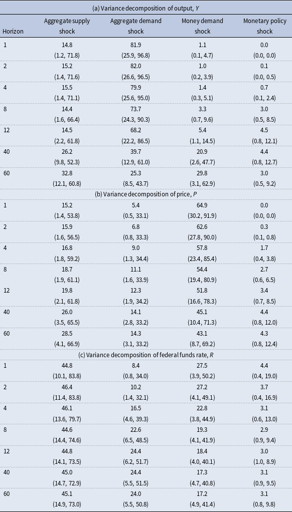
In Table A.1, I report FEVDs for the pre-IOR period up to a 60-month horizon. The three subtables report the decomposition for output, the price level, and the federal funds rate. The decomposition for the monetary base is in Table 3. The “center” estimates for each variable at horizon
 $h$
, where
 $h = 1,\ldots ,60$
, represent the percentage of variance of the
 $h$
-month-ahead forecast error due to the respective shocks. Because the FEVDs are highly asymmetrical from the Monte Carlo integration process, I use medians for the estimates instead of means. Thus, the center estimates do not add up to 100% for most horizons. The numbers in the parentheses represent one-standard-deviation error bands.Footnote
11
Table A.1(a) reports the variance decomposition of
 $Y$
. Much of the variability in
 $Y$
comes from the aggregate demand shock at short and medium horizons. Over longer horizons, aggregate supply accounts for 32.8% by 60 months and money demand for 29.8%. In Table A.1(b), money demand shocks account for most of the fluctuations in the price level at shorter horizons and still account for 43.1% at 60 months. Aggregate demand shocks account for approximately 14% of this variation in the long run. Monetary policy shocks account for no more than 4.5% of the variation in
 $Y$
and no more than 4.4% of the variation in
 $P$
at any horizon reported. Table A.1(c) reports the FEVDs for
 $R$
. Aggregate supply accounts for approximately 45% of the variation in the federal funds rate at every horizon reported.
I present the IRFs to shocks in the post-IOR period in Figure A.2. A positive innovation in
 $Y$
raises the price level permanently, by approximately 0.16% at 60 months, with the 68% error band above zero for 34 months. That increase is smaller than its pre-IOR counterpart and more precisely estimated. The federal funds rate barely moves in response to the aggregate supply shock while the monetary base rises, which may reflect an accommodative policy stance in the face of supply-side innovations. Turning to the second column, an aggregate demand shock lowers output by approximately 0.28% on impact, with the error band below zero over the first four months, after which the response returns toward zero. The price level rises to approximately 0.20% with its band above zero for 48 months, and the federal funds rate again barely moves while the monetary base rises. The third column of Figure A.2 plots the IRFs to a money demand shock. These responses grow with the horizon rather than settling. By 60 months output reaches approximately 1.5%, the federal funds rate approximately 1.5 percentage points, and the monetary base approximately
 $-33$
%. The declining base is consistent with the Fed tightening the money supply to preempt inflationary pressures arising from the increase in money demand, and the positive output response is consistent with portfolio rebalancing, where households sell non-monetary assets to increase their money holdings and then spend the proceeds. The growth in these responses at long horizons reflects the near-unit-root dynamics of the post-IOR sample discussed in Subsection 4.1, and the error bands widen with it. Only the federal funds rate response is well determined throughout, with a band above zero at every horizon, and the monetary base band lies below zero for 26 months. I treat the remaining long-horizon money demand responses as descriptive.
Pre-IOR—FEVDs
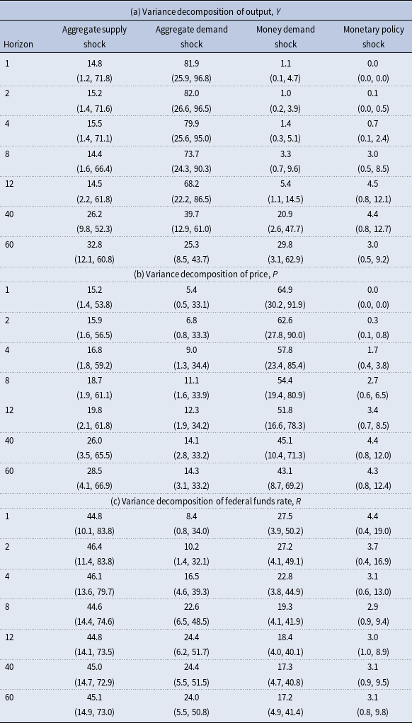
Table A1. Long description
The table presents variance decomposition data for output, price, and federal funds rate across different shocks and horizons. It is divided into three sections: (a) Variance decomposition of output, (b) Variance decomposition of price, and (c) Variance decomposition of federal funds rate. Each section lists values for different horizons (1, 2, 4, 8, 12, 40, 60) and shocks (Aggregate supply, Aggregate demand, Money demand, Monetary policy). Section (a) shows the variance decomposition of output with values for each shock and horizon. Section (b) details the variance decomposition of price, and section (c) presents the variance decomposition of the federal funds rate. Each value is accompanied by a range in parentheses indicating the confidence interval.
Post-IOR: IRFs to identified shocks.
Notes: Cumulative IRFs to one-standard-deviation aggregate supply, aggregate demand, and money demand shocks, estimated on 2008M11–2018M10 with three lags. In each panel, the solid blue line is the mean response and the two dashed lines are 68% error bands. Vertical scales differ across panels, and the money demand column is drawn on a much wider scale than the other two.

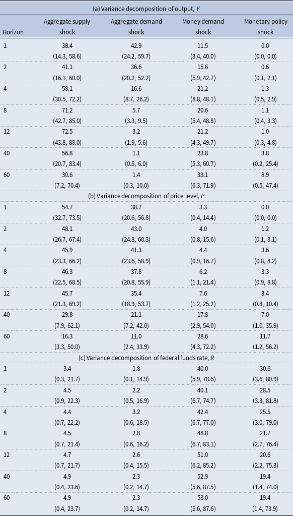
Table A.2 reports the FEVDs for the post-IOR period, which measure the variability in the forecast errors of the variables due to structural shocks. The composition differs from the pre-IOR period at every horizon. In Table A.2(a), aggregate demand and aggregate supply shocks together account for just over 80% of the variation in output on impact, at 42.9 and 38.4%. Aggregate supply reaches 72.5% at a year and falls to 30.6% by 60 months, where money demand accounts for 33.1%. In Table A.2(b), aggregate supply accounts for 54.7% and aggregate demand for 38.7% of price-level variation on impact, with money demand rising to 28.6% by 60 months. In Table A.2(c), money demand shocks account for 40.0% of the variation in the federal funds rate on impact, rising to 53.0% at 60 months, while the monetary policy share falls from 30.6 to 19.4%. As with the monetary base decomposition, these post-IOR shares are estimated imprecisely, with one-standard-deviation bands spanning most of the range at longer horizons, so I treat the comparison as descriptive.
Post-IOR—FEVDs
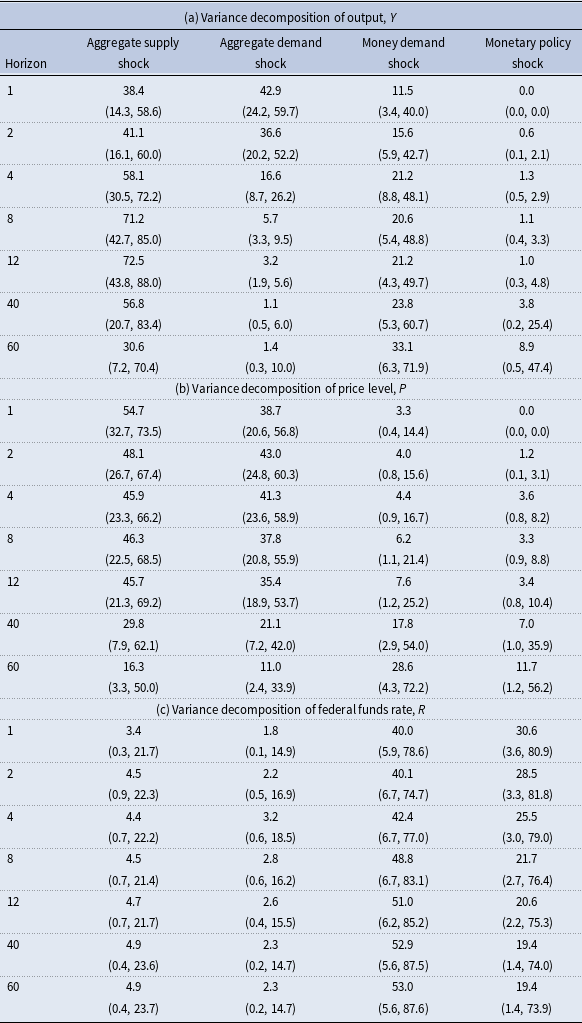
Table A2. Long description
The table presents variance decompositions of output, price level, and federal funds rate due to aggregate supply, aggregate demand, money demand, and monetary policy shocks. It is divided into three sections: (a) Variance decomposition of output, (b) Variance decomposition of price level, and (c) Variance decomposition of federal funds rate. Each section lists values for different horizons (1, 2, 4, 8, 12, 40, 60 months) and includes one-standard-deviation ranges. Section (a) shows how different shocks contribute to the variation in output over time. Section (b) illustrates the contribution of shocks to the variation in the price level. Section (c) depicts the contribution of shocks to the variation in the federal funds rate. Each row lists the horizon, followed by the percentage contributions of each shock type and their respective one-standard-deviation ranges.
B. Necessary and sufficient conditions of identification scheme
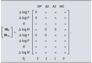
The SVAR employed in the paper is identified using both short- and long-run restrictions. Table B.1 presents the identification scheme of the model. Here, I verify that the model satisfies Rubio-Ramirez et al. (Reference Rubio-Ramirez, Waggoner and Zha2010)’s sufficient condition for global identification. The sufficient rank condition is satisfied if all the associated rank matrices have full rank. Rubio-Ramirez et al. (Reference Rubio-Ramirez, Waggoner and Zha2010) also argue that organizing the columns such that those with the most restrictions appear first is the most efficient way to check the rank condition. Without loss of generality, this is represented in Table B.1 below.
Identifying restrictions
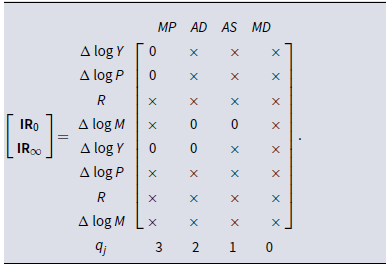
Table B1. Long description
A matrix with six rows and six columns, displaying correlation values between various economic indicators. The rows and columns are labeled with economic variables such as delta log Y, delta log P, R, delta log M, and delta log Y, delta log P, R, delta log M. The matrix is symmetrical with zeros along the diagonal. The columns are labeled MP, AD, AS, and MD. Notable trends include specific zeros and crosses indicating restrictions in the model. The matrix verifies the identification scheme of the model by checking the rank condition.
Following the notation in Rubio-Ramirez et al. (Reference Rubio-Ramirez, Waggoner and Zha2010),
 $MP$
represents a monetary policy shock,
 $AD$
represents an aggregate demand shock,
 $AS$
stands for aggregate supply shock, and
 $MD$
is a money demand shock. The symbol
 $\times$
denotes unrestricted parameters while
 $0$
represents zero restrictions imposed. The number of restrictions
 $(\sum _{j=1}^{4} q_{j} = 6)$
is equal to
 $n(n-1)/2=6$
so Rothenberg (Reference Rothenberg1971)’s necessary order condition for identification holds.
According to Theorem 7 in Rubio-Ramirez et al. (Reference Rubio-Ramirez, Waggoner and Zha2010), this model is exactly identified because
 $q_j = n - j$
for
 $j = 1, \ldots , 4$
.Footnote
12
I now express the restriction matrices
 $Q_j$
for
 $j = 1, \ldots , 4$
as
 \begin{equation*} \mathbf{Q}_{1}=\left [\begin{array}{cccccccc} 1 & 0 & 0 & 0 & 0 & 0 & 0 & 0\\ 0 & 1 & 0 & 0 & 0 & 0 & 0 & 0\\ 0 & 0 & 0 & 0 & 1 & 0 & 0 & 0\\ \ldots & \ldots & \ldots & \ldots & \ldots & \ldots & \ldots & \ldots \\ 0 & 0 & 0 & 0 & 0 & 0 & 0 & 0 \\ 0 & 0 & 0 & 0 & 0 & 0 & 0 & 0 \\ 0 & 0 & 0 & 0 & 0 & 0 & 0 & 0 \\ 0 & 0 & 0 & 0 & 0 & 0 & 0 & 0 \\ 0 & 0 & 0 & 0 & 0 & 0 & 0 & 0 \\ \end{array}\right ], \mathbf{Q}_{2}=\left [\begin{array}{cccccccc} 0 & 0 & 0 & 1 & 0 & 0 & 0 & 0\\ 0 & 0 & 0 & 0 & 1 & 0 & 0 & 0\\ \ldots & \ldots & \ldots & \ldots & \ldots & \ldots & \ldots & \ldots \\ 0 & 0 & 0 & 0 & 0 & 0 & 0 & 0 \\ 0 & 0 & 0 & 0 & 0 & 0 & 0 & 0 \\ 0 & 0 & 0 & 0 & 0 & 0 & 0 & 0 \\ 0 & 0 & 0 & 0 & 0 & 0 & 0 & 0 \\ 0 & 0 & 0 & 0 & 0 & 0 & 0 & 0 \\ 0 & 0 & 0 & 0 & 0 & 0 & 0 & 0 \\ \end{array}\right ] \end{equation*}
 \begin{equation*} \mathbf{Q}_{3}=\left [\begin{array}{cccccccc} 0 & 0 & 0 & 1 & 0 & 0 & 0 & 0\\ \ldots & \ldots & \ldots & \ldots & \ldots & \ldots & \ldots & \ldots \\ 0 & 0 & 0 & 0 & 0 & 0 & 0 & 0 \\ 0 & 0 & 0 & 0 & 0 & 0 & 0 & 0 \\ 0 & 0 & 0 & 0 & 0 & 0 & 0 & 0 \\ 0 & 0 & 0 & 0 & 0 & 0 & 0 & 0 \\ 0 & 0 & 0 & 0 & 0 & 0 & 0 & 0 \\ 0 & 0 & 0 & 0 & 0 & 0 & 0 & 0 \\ 0 & 0 & 0 & 0 & 0 & 0 & 0 & 0 \\ \end{array}\right ]\: \text{and} \: \: \mathbf{Q}_{4}=\left [\begin{array}{cccccccc} 0 & 0 & 0 & 0 & 0 & 0 & 0 & 0 \\ 0 & 0 & 0 & 0 & 0 & 0 & 0 & 0 \\ 0 & 0 & 0 & 0 & 0 & 0 & 0 & 0 \\ 0 & 0 & 0 & 0 & 0 & 0 & 0 & 0 \\ 0 & 0 & 0 & 0 & 0 & 0 & 0 & 0 \\ 0 & 0 & 0 & 0 & 0 & 0 & 0 & 0 \\ 0 & 0 & 0 & 0 & 0 & 0 & 0 & 0 \\ 0 & 0 & 0 & 0 & 0 & 0 & 0 & 0 \\ \end{array}\right ]. \end{equation*}
Finally, fill the rank matrices
 $M_j$
for
 $j = 1, \ldots , 4$
as
 \begin{equation*} \begin{aligned} & \mathbf{M}_{1}=\left [\begin{array}{cccc} 0 & \times & \times & \times \\ 0 & \times & \times & \times \\ 0 & 0 & \times & \times \\ \cdots & \cdots & \cdots & \cdots \\ 0 & 0 & 0 & 0 \\ 0 & 0 & 0 & 0 \\ 0 & 0 & 0 & 0 \\ 0 & 0 & 0 & 0 \\ 0 & 0 & 0 & 0 \\ \cdots & \cdots & \cdots & \cdots \\ 1 & 0 & 0 & 0 \end{array}\right ], & \mathbf{M}_{2}=\left [\begin{array}{cccc} \times & 0 & 0 & \times \\ 0 & 0 & \times & \times \\ \cdots & \cdots & \cdots & \cdots \\ 0 & 0 & 0 & 0 \\ 0 & 0 & 0 & 0 \\ 0 & 0 & 0 & 0 \\ 0 & 0 & 0 & 0 \\ 0 & 0 & 0 & 0 \\ 0 & 0 & 0 & 0 \\ \cdots & \cdots & \cdots & \cdots \\ 1 & 0 & 0 & 0 \\ 0 & 1 & 0 & 0 \end{array}\right ], \\ & \mathbf{M}_{3}=\left [\begin{array}{cccc} \times & 0 & 0 & \times \\ \cdots & \cdots & \cdots & \cdots \\ 0 & 0 & 0 & 0 \\ 0 & 0 & 0 & 0 \\ 0 & 0 & 0 & 0 \\ 0 & 0 & 0 & 0 \\ 0 & 0 & 0 & 0 \\ 0 & 0 & 0 & 0 \\ 0 & 0 & 0 & 0 \\ \cdots & \cdots & \cdots & \cdots \\ 1 & 0 & 0 & 0 \\ 0 & 1 & 0 & 0 \\ 0 & 0 & 1 & 0 \\ \end{array}\right ]\: \: \text{and} \: \: & \mathbf{M}_{4}=\left [\begin{array}{cccc} 0 & 0 & 0 & 0 \\ 0 & 0 & 0 & 0 \\ 0 & 0 & 0 & 0 \\ 0 & 0 & 0 & 0 \\ 0 & 0 & 0 & 0 \\ 0 & 0 & 0 & 0 \\ 0 & 0 & 0 & 0 \\ 0 & 0 & 0 & 0 \\ \cdots & \cdots & \cdots & \cdots \\ 1 & 0 & 0 & 0 \\ 0 & 1 & 0 & 0 \\ 0 & 0 & 1 & 0 \\ 0 & 0 & 0 & 1 \\ \end{array}\right ]. \end{aligned} \end{equation*}
It is straightforward to verify that all the rank matrices above are full rank. Thus the conditions of Rubio-Ramirez et al. (Reference Rubio-Ramirez, Waggoner and Zha2010)’s theorem 1 are satisfied and the model is globally identified.
C. Robustness checks
I report three robustness checks for the post-IOR results. Subsection C.1 addresses the unequal lengths of the two subsamples and the near-coincidence of the IOR introduction with the financial crisis, the two identification concerns that matter most for interpreting the muted responses. Subsection C.2 extends the post-IOR sample through 2025M12 and tests for a structural break at the 2018M10 endpoint. Subsection C.3 replaces the federal funds rate with the IOR-FFR spread.
C.1. Subsample length and the financial crisis
The post-IOR sample is short relative to the pre-IOR sample, 120 observations against 502, and the introduction of IOR nearly coincides with the 2008 financial crisis. Both raise the same question, whether the muted post-IOR responses reflect a change in transmission or a property of the estimation window.
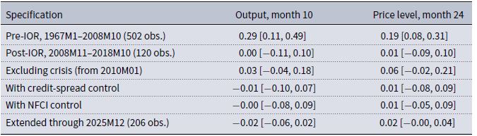
Table C.1 places every specification on one scale, the response to a monetary policy shock that raises the monetary base by 1% on impact. I rescale because a one-standard-deviation shock is not the same experiment in the two regimes. It moves the base by roughly 1.8% after 2008 against 0.8 to 1.1% in pre-IOR windows, so the raw responses are not comparable across periods. On the common scale the post-IOR band is narrower than the pre-IOR band, and narrower still under the financial-stress controls and in the extended sample. Precision comes from the size of the policy-driven movements of the base, and the post-IOR period contains the largest such movements in the sample.
Responses per 1% expansion of the monetary base
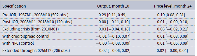
Table C1. Long description
A table with six rows and three columns. The columns are labeled Specification, Output, month 10, and Price level, month 24. The rows are labeled with different specifications and their corresponding values. Row 1: Pre-IOR, 1967M1-2008M10 (502 obs.), 0.29 [0.11, 0.49], 0.19 [0.08, 0.31]. Row 2: Post-IOR, 2008M11-2018M10 (120 obs.), 0.00 [-0.11, 0.10], 0.01 [-0.09, 0.10]. Row 3: Excluding crisis (from 2010M01), 0.03 [-0.04, 0.18], 0.06 [-0.02, 0.21]. Row 4: With credit-spread control, -0.01 [-0.10, 0.07], 0.01 [-0.08, 0.09]. Row 5: With NFCI control, 0.00 [-0.08, 0.09], 0.01 [-0.05, 0.09]. Row 6: Extended through 2025M12 (206 obs.), 0.02 [-0.06, 0.02], 0.02 [-0.00, 0.04].
Notes: Median responses to a monetary policy shock, rescaled within each posterior draw so that the shock raises the monetary base by 1% on impact, with 68% error bands in brackets. The pre-IOR specification uses five lags and the post-IOR specifications three. The extended-sample row is the specification of Appendix C.2, which includes the post-2018M10 regime dummy and the COVID dummy.
Equal-length windows confirm that 120 observations suffice to detect transmission where it exists. The 1978M11–1988M10 window matches the post-IOR sample in length and covers a period during which the Federal Reserve targeted nonborrowed reserves. Estimated on that window, the model yields a price-level response whose 68% band excludes zero for 59 months and an output response significant for 22 months. Equal-length windows drawn from the Great Moderation do not recover significant transmission, which is what passive reserve supply under funds-rate targeting implies, since the base moved little over those years. Adding observations works the same way. The extended sample of Subsection C.2 raises the post-IOR sample from 120 observations to 206, and the output response stays muted while its band narrows.
The crisis is harder to separate from IOR, since the two are three weeks apart, and I do not claim to separate them fully. Three exercises nonetheless indicate that the muted responses are not a crisis artifact. Re-estimating on 2010M01–2018M10, which excludes the acute crisis entirely, leaves the responses muted. Augmenting every equation of both regimes with a financial-stress indicator and its lags leaves the stability test undiminished, with
 $LR = 898.6$
using the Baa–Aaa default spread and
 $LR = 878.8$
using the Chicago Fed National Financial Conditions Index, against
 $LR = 883.2$
without controls. The timing is informative as well. Financial stress normalized within roughly two years of the Lehman failure, with the Baa–Aaa spread peaking in December 2008 and returning to its historical range by 2010, while the muted transmission persists through the end of the sample. Precautionary liquidity hoarding could account for 2009, but not for 2017. I therefore interpret the results as consistent with the IOR regime, and they do not establish that IOR alone caused the change.
C.2. Extended post-IOR sample (2008M11–2025M12)
The baseline post-IOR sample ends in October 2018. Extending it through December 2025 adds 86 observations, which raises the post-IOR sample from 120 to 206, and allows a test of whether that endpoint is the right one. The extended sample introduces two complications. First, after October 2018 the IOR-FFR spread collapses to zero and turns negative, so the post-2018 observations do not satisfy the condition (IOR
 $\gt$
FFR) that defines the baseline post-IOR regime. Second, the COVID-19 pandemic (March–June 2020) produced extreme outliers in industrial production, the federal funds rate, and the monetary base.
To address these issues, the extended-sample SVAR includes two exogenous dummy variables in the deterministic block: a post-2018 regime dummy (equal to one from 2018M11 onward) and a COVID dummy (equal to one for 2020M3–2020M6).Footnote 13 These dummy variables absorb the associated level shifts without altering the structural identification.
Before estimating the SVAR, I conduct a Chow-type likelihood ratio test for a structural break at 2018M10. The test compares the log-determinant of the residual covariance matrix from a VAR estimated over the full extended sample with those from VARs estimated separately on the 2008M11–2018M10 and 2018M11–2025M12 subsamples. Under the null hypothesis of parameter stability, the test statistic is distributed
 $\chi ^2$
with
 $n_{\text{var}} \times (n_{\text{var}} \times p + 1) = 52$
degrees of freedom, where
 $n_{\text{var}} = 4$
and
 $p = 3$
.
The Chow LR statistic is 473.73 (df = 52), far exceeding the 5% critical value of 69.83, with a
 $p$
-value effectively equal to zero (
 $p \lt 10^{-62}$
). This decisively rejects the null hypothesis of parameter stability at 2018M10. The Chow test confirms instability without identifying its source, and the collapse of the IOR-FFR spread after October 2018 provides a theoretically grounded explanation for the break, supporting the baseline sample split.
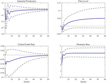
Figure C.1 displays the IRFs to a monetary policy shock from the extended-sample SVAR. The responses are qualitatively similar to the baseline post-IOR results, with output and the price level remaining muted and statistically imprecise and 68% error bands encompassing zero at most horizons. Per 1% expansion of the monetary base, the output response is
 $-0.02$
with a band of
 $[\!-0.06, 0.02]$
and the price-level response is
 $0.02$
with a band of
 $[\!-0.00, 0.04]$
, reported in Table C.1. The additional 86 observations narrow the bands without reviving transmission.
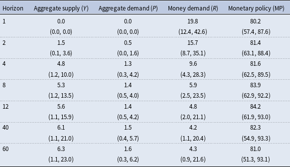
Table C.2 reports the FEVD of the monetary base for this specification. Monetary policy shocks account for 80% of base variation on impact, substantially higher than the 51% in the baseline post-IOR specification. The difference is expected, because the intercept dummies absorb variation associated with the post-2018 regime change and COVID disruptions that would otherwise show up in the money demand shock, which mechanically inflates the monetary policy share. Since the dummies cannot account for the slope instability confirmed by the Chow test, the baseline sample split remains the appropriate specification.
Extended sample decomposition of variance for the monetary base
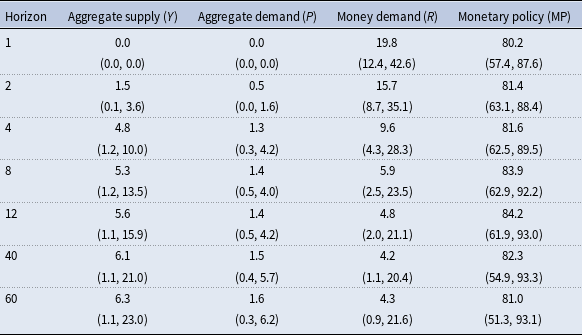
Table C2. Long description
A table showing the decomposition of variance for the monetary base across different horizons. The table has 10 rows and 4 columns. The columns are labeled Horizon, Aggregate supply (Y), Aggregate demand (P), Money demand (R), and Monetary policy (MP). Each row represents a different horizon value (1, 2, 4, 8, 12, 40, 60) and includes corresponding values for Aggregate supply, Aggregate demand, Money demand, and Monetary policy. For example, Row 1: Horizon 1, Aggregate supply (0.0, (0.0, 0.0)), Aggregate demand (0.0, (0.0, 0.0)), Money demand 19.8, (12.4, 42.6), Monetary policy 80.2, (57.4, 87.6).
Notes: Extended sample forecast error variance decomposition of the monetary base. The numbers represent the median percentage of forecast error variance explained by each structural shock. 68% confidence intervals are reported in parentheses.
Robustness: IRFs to monetary policy shock—extended sample (2008M11–2025M12).
Notes: Cumulative impulse responses to a one-standard-deviation monetary policy shock, estimated on 2008M11–2025M12. The model includes a post-2018M10 regime dummy and a COVID dummy (2020M3–2020M6) as exogenous deterministics. The solid blue line is the mean response, and the dashed black lines are 68% error bands.

C.3. IOR-FFR spread specification (2008M11–2018M10)
The baseline specification includes the federal funds rate as the interest rate variable. As an alternative, I replace the FFR with the IOR-FFR spread in position 3 of the VAR. The spread captures the opportunity cost of holding reserves more closely, because in the post-IOR environment the relevant margin for bank portfolio decisions is the differential between the administered rate on reserves and the prevailing market rate. The spread is positive throughout the 2008M11–2018M10 sample (ranging from +0.55 percentage points in November 2008 to +0.01 in October 2018), so there is no sign-change issue within the estimation window.
The short-run and long-run restriction matrices are identical to those in the baseline. This is justified because the spread plays the same theoretical role as the FFR in the identification. It enters the money demand equation as an opportunity cost variable, and it does not enter the production-sector equations contemporaneously.
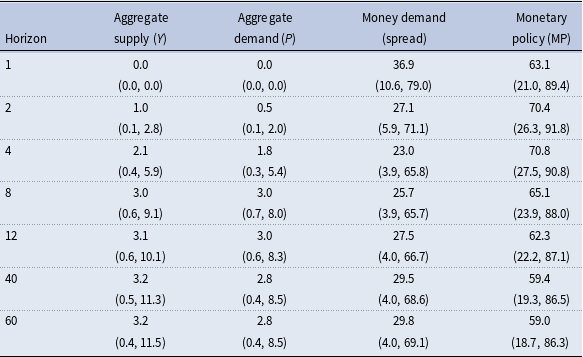
Figure C.2 displays the impulse responses. The results are qualitatively consistent with the baseline. Output and price-level responses to the monetary policy shock remain muted and statistically insignificant. Table C.3 reports the monetary base variance decomposition. Monetary policy shocks account for 63% of monetary base variation on impact, more than in the baseline FFR specification (51%) but substantially less than the 86% observed in the pre-IOR period.
Robustness (spread model): decomposition of variance for the monetary base

Table C3. Long description
A table titled ‘Robustness (spread model): decomposition of variance for the monetary base’ with data on aggregate supply, aggregate demand, money demand spread, and monetary policy across various horizons. The table has 7 rows and 4 columns. Column headers are Horizon, Aggregate supply (Y), Aggregate demand (P), Money demand (spread), and Monetary policy (MP). Row labels include horizons at 1, 2, 4, 8, 12, 40, and 60. Each cell contains values and confidence intervals in parentheses. For example, Row 1: Horizon 1, Aggregate supply (0.0), Aggregate demand (0.0), Money demand (36.9), Monetary policy (63.1). Row 2: Horizon 2, Aggregate supply (1.0), Aggregate demand (0.5), Money demand (27.1), Monetary policy (70.4). The table provides a detailed variance decomposition of the monetary base, showing how different factors contribute to its variation over time.
Notes: Robustness check (2008M11–2018M10) forecast error variance decomposition of the monetary base, replacing the federal funds rate with the IORB-FFR spread. The numbers represent the median percentage of forecast error variance explained by each structural shock. 68% confidence intervals are reported in parentheses.
Robustness: IRFs to monetary policy shock—IOR-FFR spread model (2008M11–2018M10).
Notes: Cumulative impulse responses to a one-standard-deviation monetary policy shock. The IORB-FFR spread replaces the federal funds rate in position 3 of the VAR. The solid blue line is the mean response, and the dashed black lines are 68% error bands.



 M
 M