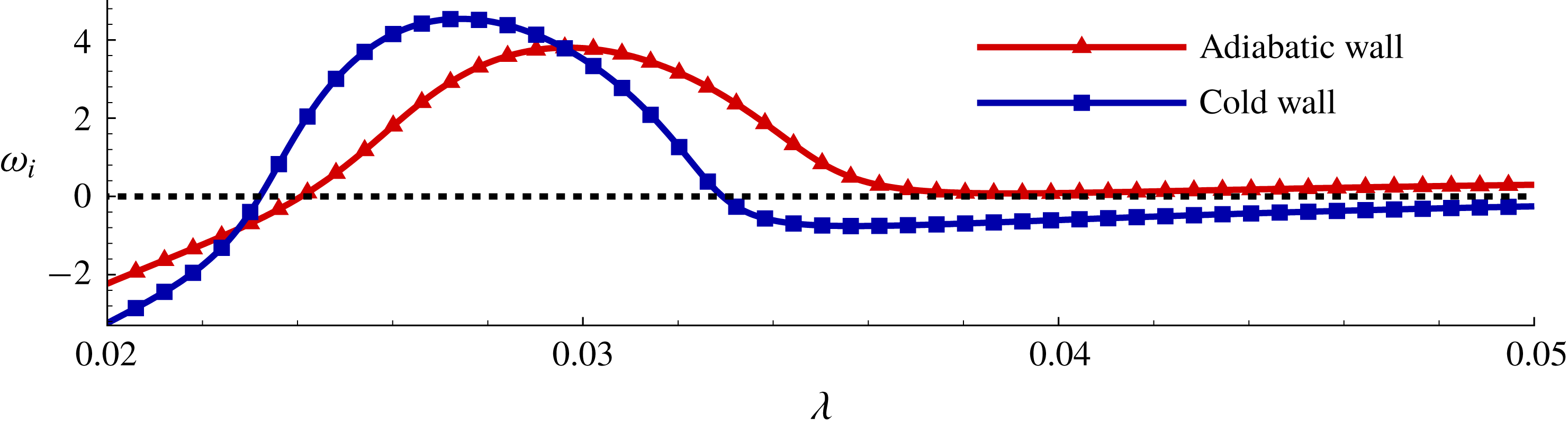
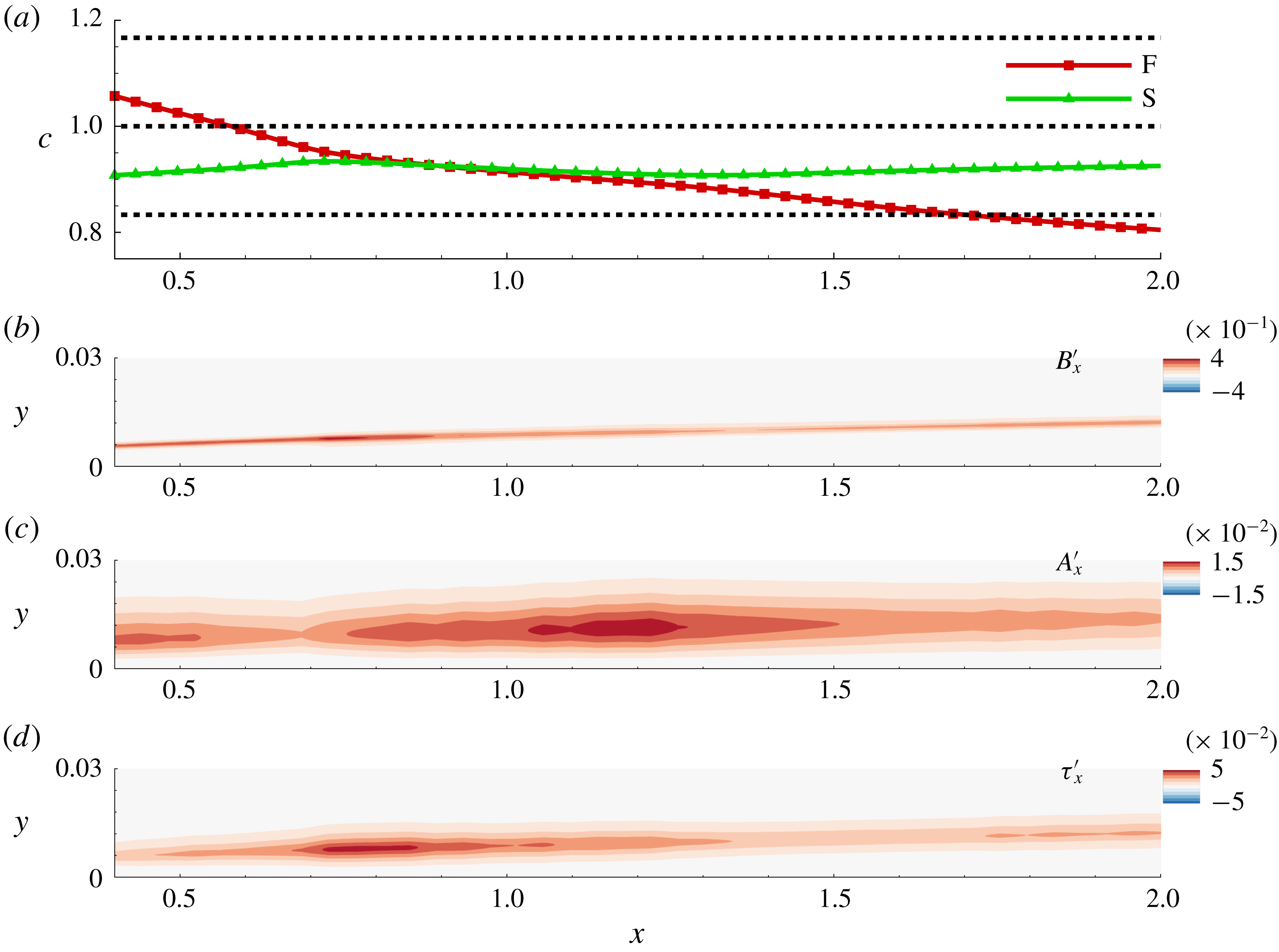
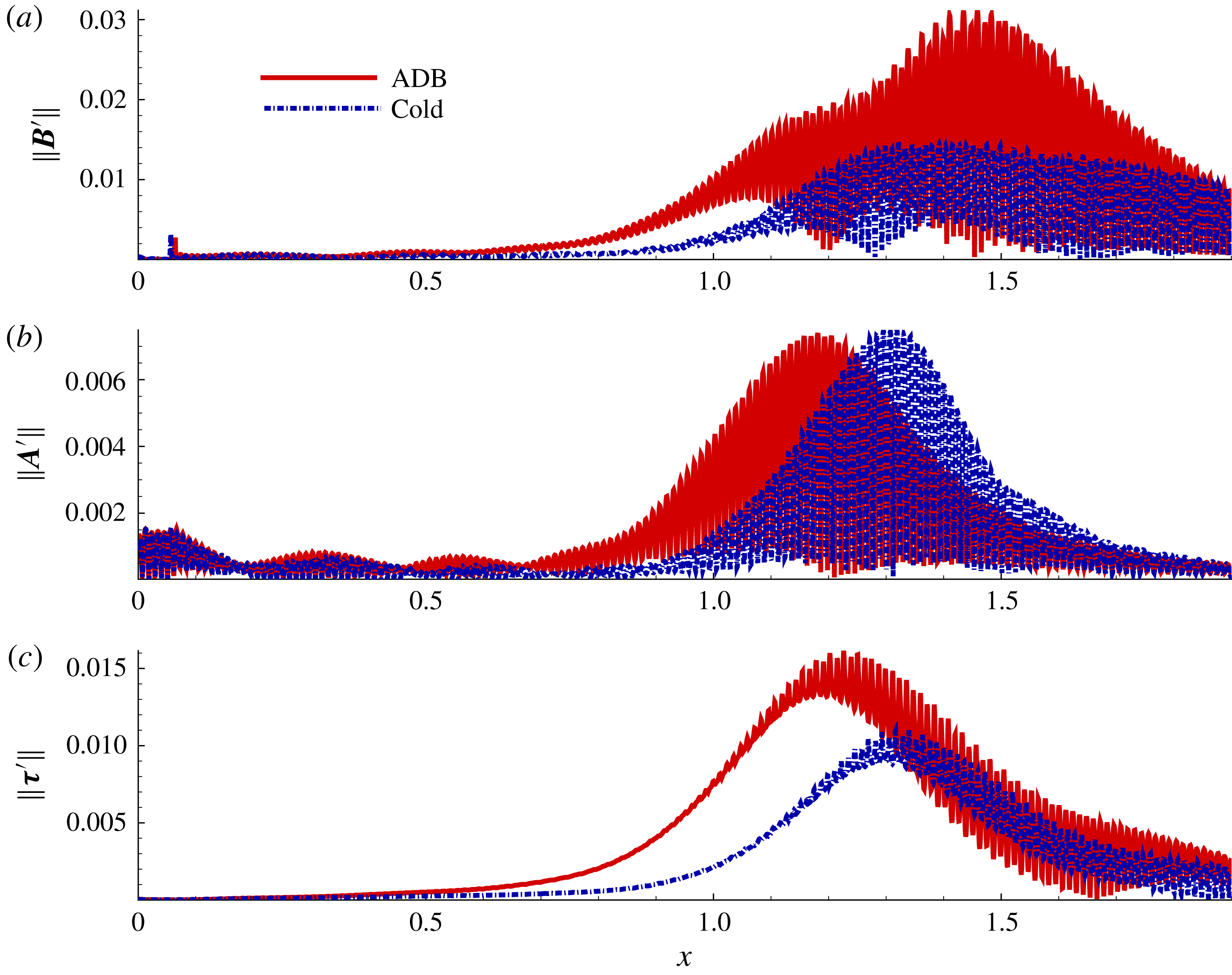
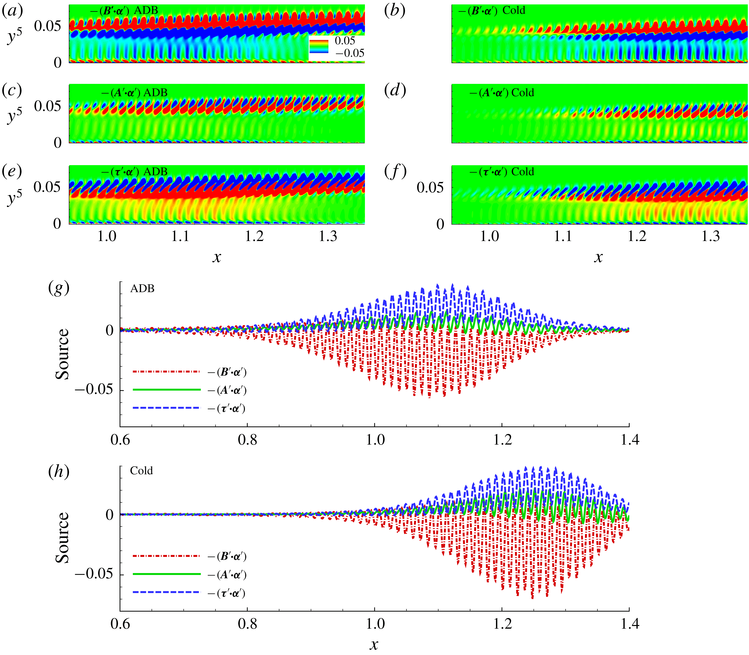
1 Introduction
The design of future supersonic and hypersonic air vehicles will be greatly improved through better understanding of transition in high-speed boundary layers. Transition, and subsequent turbulence, is associated with increased skin friction and drag, higher heating loads and degradation of control surface effectiveness. Key phenomena of interest include receptivity and subsequent perturbation growth, which are sensitive to several parameters, including free-stream Mach number (
 $M_{\infty }$
), Reynolds number (
 $Re$
), thermal boundary conditions, physical character of the disturbances and shocks (Reshotko Reference Reshotko1976). Higher Mach numbers engender new modes of instability, along with inter-modal interactions in the linear as well as nonlinear regimes of perturbation growth. This rich dynamics poses constraining challenges in understanding and predicting transition in high-speed flows, and inhibits the effort to develop effective control strategies.
Numerous experimental investigations (e.g. Kosinov, Maslov & Shevelkov Reference Kosinov, Maslov and Shevelkov1990; Stetson & Kimmel Reference Stetson and Kimmel1993; Schneider Reference Schneider2001; Kennedy et al.
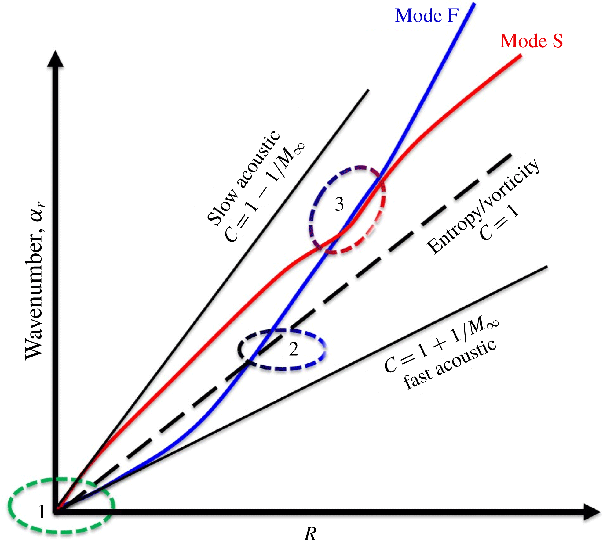
Reference Kennedy, Laurence, Smith and Marineau2018), linear stability analyses (e.g. Mack Reference Mack1975, Reference Mack1984; Malik Reference Malik1990) and direct numerical simulations (e.g. Erlebacher & Hussaini Reference Erlebacher and Hussaini1990; Zhong Reference Zhong2001; Zhong & Wang Reference Zhong and Wang2012)) have yielded significant insight into various transition mechanisms in high-speed flows. Reshotko (Reference Reshotko2008) reviews several pathways to turbulence as governed by the perturbation environment and the receptivity of the boundary layer. An important parameter in the initial stages of hypersonic boundary layer (HBL) instability growth is the phase speed of the instability wave (Fedorov Reference Fedorov2011; Zhong & Wang Reference Zhong and Wang2012). The considerations are summarized using figure 1, adapted from Fedorov (Reference Fedorov2011), which depicts the evolution of instability modes in an HBL, at a fixed frequency, in the context of a flat-plate geometry. The ordinate represents the real part of the wavenumber,
 $\unicode[STIX]{x1D6FC}_{r}$
, while the abscissa is the Reynolds number,
 $R=\sqrt{U_{e}^{\ast }x^{\ast }/\unicode[STIX]{x1D708}_{e}^{\ast }}$
, based on the Blasius length scale,
 $\sqrt{\unicode[STIX]{x1D708}_{e}^{\ast }x^{\ast }/U_{e}^{\ast }}$
. Here
 $\unicode[STIX]{x1D708}_{e}^{\ast }$
and
 $U_{e}^{\ast }$
are the kinematic viscosity and streamwise velocity at the outer edge of the boundary layer, respectively, at a distance of
 $x^{\ast }$
from the leading edge. All starred quantities
 $(\cdot )^{\ast }$
represent dimensional variables. The slope,
 $\unicode[STIX]{x1D6FC}_{r}/R=F/c$
, is the phase speed,
 $c$
, of the wave, defined as
 $c=\unicode[STIX]{x1D714}/\unicode[STIX]{x1D6FC}$
, where
 $\unicode[STIX]{x1D714}$
is the non-dimensional circular frequency, and the non-dimensional frequency parameter,
 $F=\unicode[STIX]{x1D714}^{\ast }\unicode[STIX]{x1D708}_{e}^{\ast }/{U_{e}^{\ast }}^{2}$
. The slopes of the black straight lines represent phase speeds of the slow and fast acoustic as well as entropy and vorticity waves. The normalized phase speeds of these are marked in figure 1: at zero angle of incidence, the acoustic waves travel at
 $c=1-1/M_{\infty }$
(slow) and
 $c=1+1/M_{\infty }$
(fast), while the other two convect (
 $c=1$
). Coloured lines represent the evolution of key stability modes, including ‘mode F’ and ‘mode S’. The terminology employed to identify these has been the subject of discussion in the literature (Fedorov & Tumin Reference Fedorov and Tumin2011). For consistency in the ensuing discussion, we follow Fedorov (Reference Fedorov2011).
Evolution of waves in a hypersonic boundary layer. Black lines represent fast acoustic, slow acoustic and vortical/entropic waves (
 $c$
represents wave speed). Coloured lines represent stability modes: mode S and mode F, corresponding to the stability modes that originate with the phase speeds of the slow and fast acoustic waves, respectively, near the leading edge. Adapted from Fedorov (Reference Fedorov2011).

Phase speed synchronization locations are marked 1, 2 and 3, respectively. Each is associated with phenomena of interest. In region 2, mode F synchronizes with the vortical and entropic waves of the continuous spectra: at this point, mode F is susceptible to free-stream turbulence (vortical) and hotspots (entropic) (Fedorov & Tumin Reference Fedorov and Tumin2003). In region 3, fast–slow (FS) synchronization occurs: here the nature of mode S changes in a manner absent in incompressible or low-supersonic boundary layers. Specifically, mode S morphs from the first (Tollmien–Schlichting or TS mode, also observed in incompressible boundary layers) to the second (or Mack) mode. The two-dimensional form of the second mode exhibits higher growth rates than the TS wave, thus becoming the crucial trigger of hypersonic transition by initiating nonlinear saturation and breakdown in the boundary layer. Multiple such higher unstable modes were originally reported by Mack (Reference Mack1975, Reference Mack1984): they arise in boundary layers above
 $M_{\infty }=3$
(e.g. Özgen & Kırcalı Reference Özgen and Kırcalı2008). Second and higher Mack modes are inherently inviscid instabilities and are sensitive to wall and free-stream thermal conditions. Fedorov (Reference Fedorov2011) describes the evolution of the second mode in terms of a waveguide, where the wave is trapped in a region between the wall and the sonic line.
As noted above, the black lines in figure 1 identify perturbations through their vortical (also designated hydrodynamic), acoustic and thermal (or entropic) characteristics. As opposed to stability modes, these are more naturally identified with a Kovásznay-type classification (Kovásznay Reference Kovásznay1953). There are several ways to perform a decomposition of flow perturbations in this manner, depending on the definition and procedure employed. For reasons outlined below, we avoid the definitions and approach delineated in Kovásznay (Reference Kovásznay1953): to emphasize this distinction, we designate vortical, acoustic and thermal perturbations as fluid-thermodynamic (FT) components. We also do not use the term ‘mode’ for these components, as in Unnikrishnan & Gaitonde (Reference Unnikrishnan and Gaitonde2016), to avoid confusion with stability modes. Likewise, the term ‘fluctuation’ will be reserved for the difference between instantaneous and mean values of raw quantities.
Phase speeds (slopes) near the leading edge (region 1 of figure 1) have been used to associate stability modes with their FT character (Fedorov & Khokhlov Reference Fedorov and Khokhlov1991; Fedorov Reference Fedorov2003). Thus, mode S aligns with the slow acoustic wave (both having phase speed
 $1-1/M_{\infty }$
), and mode F aligns with the fast acoustic wave (phase speed
 $1+1/M_{\infty }$
) (Fedorov & Khokhlov Reference Fedorov and Khokhlov1991, Reference Fedorov and Khokhlov1992). Similarly, the asymptotic free-stream behaviour of modes with phase speeds close to unity corresponds to transport of entropy and vorticity. Additional discussions in like vein may be found, for example, in Wang, Zhong & Ma (Reference Wang, Zhong and Ma2011).
It is evident from a study of the eigenspectra, however, that the direct connection between acoustic modes and corresponding FT components only holds near the leading edge; at downstream locations, the phase speeds of mode S and mode F deviate from those of the physical waves in figure 1. Nonetheless, the literature on hypersonic transition dynamics describes the subsequent evolution of stability modes by weaving FT component terminology, but not in a rigorous manner. For example, the synchronization of phase speeds of mode F and mode S is said to be associated with a change in the vortical character of the first-mode instability (or TS mode) into the second or Mack mode (Ma & Zhong Reference Ma and Zhong2003a ), which is traditionally understood as having an acoustic nature. However, the vortical, acoustic and thermal content of all stability modes evolve and interact with each other in the downstream direction in dynamically significant ways.
The goal of this paper is to describe the key processes associated with aspects of modal growth (figure 1) in terms of FT components. We seek specifically to analyse phenomena during synchronization events in this manner to augment the stability perspective discussed, for example, in Fedorov (Reference Fedorov2011) and Fedorov & Tumin (Reference Fedorov and Tumin2011). The advantage of such a description is clear: FT components are subject to laws that govern their interactions with each other and with the mean flow. It thus provides a causal qualitative and quantitative understanding of perturbation evolution that is difficult to obtain from stability analyses. For example, the FS synchronization process, which changes the nature of the most unstable mode, is accompanied by characteristic changes in the relative composition of vortical, acoustic and thermal components (§ 4.2). Likewise, in addition to the sensitivity to thermal hotspots mentioned above (Fedorov & Tumin Reference Fedorov and Tumin2003), discussed in § 4.2, effects of wall conditions highlight the importance of the thermal component (§ 5.7). Furthermore, although this paper is scoped only to a subset of transition processes (including saturated nonlinear growth, § 5.6), the approach is capable of seamlessly treating upstream receptivity processes (Ma & Zhong Reference Ma and Zhong2003a ,Reference Ma and Zhong b , Reference Ma and Zhong2005) as well as downstream resonant interactions and breakdown into turbulence (Sivasubramanian & Fasel Reference Sivasubramanian and Fasel2014, Reference Sivasubramanian and Fasel2015). This includes the effect of free-stream perturbations on shocks, where FT components can exchange energy with each other (Duck, Lasseigne & Hussaini Reference Duck, Lasseigne and Hussaini1995), even if the perturbation is small enough to trigger a linear response.
This effort thus complements the understanding obtained from the mathematics-based evolution of stability modes, with corresponding insights derived from physics-based FT interactions. The procedure comprises two steps. In the first step, fluctuations, which may be obtained from linear stability theory (LST) or direct numerical simulations (DNS), are decomposed into their vortical, acoustic and thermal components. For this, we use momentum potential theory (MPT) (Doak Reference Doak1989), discussed in § 2, which overcomes the severe restrictions in Kovásznay’s approach (Kovásznay Reference Kovásznay1953). Specifically, in this technique, a vector field, ‘momentum density’,
 $\unicode[STIX]{x1D70C}\boldsymbol{u}$
, is split into three components using Helmholtz decomposition. The vortical component of perturbations contains all rotational motion, while the irrotational component is divided into acoustic (irrotational and isentropic) and thermal (irrotational and isobaric) parts. It is important to note therefore that the sense in which the term ‘acoustic’ is used for a stability mode is quite different from that for the FT perturbation.
The second phase of the analysis considers the interactions (linear and nonlinear) among the different FT perturbations, as well as the mean flow. For this, as also described in § 2, MPT establishes an equation governing the evolution of total fluctuating enthalpy (TFE), i.e. the fluctuation (
 $H^{\prime }$
) of enthalpy per unit mass (
 $H$
). When the entire solution is known, say from a DNS, the budget can be evaluated, and the interactions between the modes can be delineated, even in the nonlinear regime, as we show in § 6.
The rest of the paper is structured as follows. The canonical problem employed for analysis is a flat-plate HBL at a free-stream Mach number,
 $M_{\infty }=6$
. The basic state associated with this problem is well known, and is summarized in § 3 for completeness. The simplicity of the problem and numerous studies of its eigenmodes allows for straightforward validation. Key aspects of the LST analysis are outlined in § 4.1, followed by the decomposition of the first and second modes into FT components using MPT (§ 4.2). Emphasis is placed on changes occurring during the FS synchronization process. Subsequently, to account for non-parallel effects, DNS are performed in the manner described in § 5.1, using forcing as in § 5.2. The decomposition of the DNS fluctuations into FT components is discussed in § 5.3. The associated FT flux patterns, and the significance of the sonic line, critical layer and generalized inflection point (GIP) are presented in § 5.4. The phase speeds of the different perturbation types, employed to motivate this work in figure 1, are examined in § 5.5. As noted above, the method extends seamlessly to the nonlinear regime – the dynamics during nonlinear saturation, including the generation of harmonics, is described in § 5.6, with emphasis on the second mode. The sensitivity of wall thermal conditions on the evolution of FT perturbation dynamics is examined in § 5.7 using both LST and DNS results. Finally, the source mechanisms responsible for the generation and dissipation of fluctuating energy in the boundary layer are evaluated under different wall thermal scenarios (§ 6).
2 Momentum potential theory
As noted earlier, the approach of Kovásznay, which assigns a different scalar variable to each component, is unsuited for extension to general flows. First, interactions between different components are difficult to address: the quadratic coupling terms considered in Chu & Kovásznay (Reference Chu and Kovásznay1958) illustrate the complexity of the treatment even in uniform base flows. A second limitation stems from the fact that, when the mean flow exhibits gradients, energy exchanges among the FT components occur even without nonlinear phenomena. An example of this can be deduced from the linearized vorticity equation, in which the baroclinic term couples the vorticity and pressure variables, leading to vortical–acoustic energy transfers. Coherent vortices can generate entropic fluctuations, and high temperature variations result in density gradients, which cause vortical perturbations (Zhou & Gore Reference Zhou and Gore1998). Thus, in an HBL, we anticipate that strong mean flow gradients near the wall and the GIP will induce significant inter-component interactions. In particular, the acoustic component in the second-mode-dominated region can receive inputs from thermal as well as vortical disturbances, whose nature and intensity depend on the Mach regime and wall thermal conditions.
The MPT approach of Doak (Reference Doak1989) overcomes these limitations and provides an elegant method to decompose fluctuations into their vortical, acoustic and thermal components. Rather than identifying each FT component with a single scalar variable, MPT selects a single vector field for this purpose, specifically momentum density,
 $\unicode[STIX]{x1D70C}\boldsymbol{u}$
. An exact decomposition, i.e. without linearizing simplifications, is then facilitated, because the continuity equation is naturally linear in
 $\unicode[STIX]{x1D70C}\boldsymbol{u}$
:
 $$\begin{eqnarray}\displaystyle \frac{\unicode[STIX]{x2202}\unicode[STIX]{x1D70C}}{\unicode[STIX]{x2202}t}+\unicode[STIX]{x1D735}\boldsymbol{\cdot }(\unicode[STIX]{x1D70C}\boldsymbol{u})=0. & & \displaystyle\end{eqnarray}$$
By definition, vortical components comprise all rotational content, while acoustic and thermal perturbations are irrotational. This step in the splitting is facilitated through a Helmholtz decomposition, which separates the rotational (solenoidal) vortical component,
 $\boldsymbol{B}$
, comprising mean (
 $\overline{\boldsymbol{B}}$
) and fluctuating (
 $\boldsymbol{B}^{\prime }$
) parts, from the irrotational component. This latter is represented as a gradient of a scalar potential
 $\unicode[STIX]{x1D713}^{\prime }$
, which contains the acoustic and thermal components:
 $$\begin{eqnarray}\displaystyle \unicode[STIX]{x1D70C}\boldsymbol{u}=\overline{\boldsymbol{B}}+\boldsymbol{B}^{\prime }-\unicode[STIX]{x1D735}\unicode[STIX]{x1D713}^{\prime },\quad \unicode[STIX]{x1D735}\boldsymbol{\cdot }\overline{\boldsymbol{B}}=0,\quad \unicode[STIX]{x1D735}\boldsymbol{\cdot }\boldsymbol{B}^{\prime }=0. & & \displaystyle\end{eqnarray}$$
The mean scalar potential
 $\overline{\unicode[STIX]{x1D713}}$
for a time-stationary flow is both irrotational and solenoidal and can thus be assumed to be zero.
Inserting (2.2) into (2.1), a Poisson equation is obtained for the scalar potential,
 $\unicode[STIX]{x1D713}^{\prime }$
:
 $$\begin{eqnarray}\displaystyle \unicode[STIX]{x1D6FB}^{2}\unicode[STIX]{x1D713}^{\prime }=\frac{\unicode[STIX]{x2202}\unicode[STIX]{x1D70C}^{\prime }}{\unicode[STIX]{x2202}t}. & & \displaystyle\end{eqnarray}$$
The total irrotational field
 $\unicode[STIX]{x1D713}^{\prime }$
is a linear combination of isentropic (acoustic) and isobaric (thermal or entropic) components. Utilizing the linear nature of (2.3), this splitting is obtained as
 $$\begin{eqnarray}\displaystyle \unicode[STIX]{x1D713}^{\prime }=\unicode[STIX]{x1D713}_{A}^{\prime }+\unicode[STIX]{x1D713}_{T}^{\prime },\quad \unicode[STIX]{x1D6FB}^{2}\unicode[STIX]{x1D713}_{A}^{\prime }=\frac{1}{a^{2}}\frac{\unicode[STIX]{x2202}p^{\prime }}{\unicode[STIX]{x2202}t},\quad \unicode[STIX]{x1D6FB}^{2}\unicode[STIX]{x1D713}_{T}^{\prime }=\frac{\unicode[STIX]{x2202}\unicode[STIX]{x1D70C}}{\unicode[STIX]{x2202}S}\frac{\unicode[STIX]{x2202}S^{\prime }}{\unicode[STIX]{x2202}t}, & & \displaystyle\end{eqnarray}$$
where
 $\unicode[STIX]{x1D735}\unicode[STIX]{x1D713}_{A}^{\prime }$
and
 $\unicode[STIX]{x1D735}\unicode[STIX]{x1D713}_{T}^{\prime }$
are the acoustic and thermal components of momentum density, respectively,
 $p$
is the thermodynamic pressure,
 $a^{2}=(\unicode[STIX]{x2202}p/\unicode[STIX]{x2202}\unicode[STIX]{x1D70C})_{S}$
is the squared value of the instantaneous local speed of sound, and
 $S$
is the entropy calculated from
 $S=S_{\infty }+c_{p}\ln (T/T_{\infty })-{\mathcal{R}}\ln (p_{\infty }/p)$
, with
 $c_{p}$
the specific heat at constant pressure and
 ${\mathcal{R}}$
the ideal gas constant.
Although the choice of the specific vector field,
 $\unicode[STIX]{x1D70C}\boldsymbol{u}$
, may appear restrictive, the above equations show that the results are dependent on
 $\unicode[STIX]{x1D70C}^{\prime }$
,
 $p^{\prime }$
and
 $S^{\prime }$
as in (2.3) and (2.4). Thus, the decomposition includes considerations of kinematic as well as thermodynamic variables, and the method is therefore quite general.
The basic procedure of FT decomposition involves obtaining the three scalar potentials,
 $\unicode[STIX]{x1D713}^{\prime },\unicode[STIX]{x1D713}_{A}^{\prime }$
and
 $\unicode[STIX]{x1D713}_{T}^{\prime }$
. For this, the Poisson equations for
 $\unicode[STIX]{x1D713}^{\prime }$
and
 $\unicode[STIX]{x1D713}_{A}^{\prime }$
are solved, requiring time derivatives of density and pressure fluctuations, respectively. Then
 $\unicode[STIX]{x1D713}_{T}^{\prime }$
is simply the difference between
 $\unicode[STIX]{x1D713}^{\prime }$
and
 $\unicode[STIX]{x1D713}_{A}^{\prime }$
. Dirichlet boundary conditions required for the Poisson equations are obtained by integration along the boundaries (Daviller, Jordan & Comte Reference Daviller, Jordan and Comte2009). The results are also confirmed by using least-squares solution of the banded matrix of the discretized equation, (2.4). The solenoidal component,
 $\boldsymbol{B}^{\prime }$
, is obtained from total momentum fluctuations,
 $(\unicode[STIX]{x1D70C}\boldsymbol{u})^{\prime }$
, since all other terms in (2.2) are then known. The exact procedure by which the splitting is performed depends to some degree on whether it is applied to the LST eigenmodes or the DNS data: these details are discussed in context below. Additional details of the implementation may be found in Unnikrishnan & Gaitonde (Reference Unnikrishnan and Gaitonde2016).
The second key component of MPT concerns the transfer of energy among FT components, which is a crucial aspect of the current work, since it provides a method to derive an energy budget as perturbations grow downstream. Thus, if a particular FT component is observed to increase in a particular region of the flow, the source terms that account for this increase can be explicitly evaluated from the DNS. As demonstrated later, this aspect of MPT can thus be used in the region of Mack-mode amplification to account for the sources responsible for the growth of the acoustic component. The choice of energy variable is the TFE,
 $H^{\prime }$
, i.e. the fluctuating component of the enthalpy per unit mass (
 $H$
), defined as
 $H=c_{p}T+\boldsymbol{u}\boldsymbol{\cdot }\boldsymbol{u}/2$
. Details of the rationale behind this choice, originally derived to examine acoustic phenomena, have been provided in Doak (Reference Doak1998). A crucial advantage is that an exact equation for the evolution of
 $H^{\prime }$
can be derived, each term of which corresponds to distinct processes to which a physical meaning can be applied.
The mean transport of TFE is obtained by considering the dot product of the momentum equation with the momentum density vector, and replacing the pressure gradient in terms of enthalpy and entropy variables using thermodynamic state relations. This yields an equation for conservation of TFE, which may be written generically in terms of fluxes, sources and sinks as
 $$\begin{eqnarray}\displaystyle \unicode[STIX]{x1D735}\boldsymbol{\cdot }[\text{flux}]=\text{sources}+\text{sinks}. & & \displaystyle\end{eqnarray}$$
Since the fluctuation
 $(\unicode[STIX]{x1D70C}\boldsymbol{u})^{\prime }$
represents a mass flux, the TFE flux is simply
 $(\unicode[STIX]{x1D70C}\boldsymbol{u})^{\prime }H^{\prime }$
. When
 $(\unicode[STIX]{x1D70C}\boldsymbol{u})^{\prime }$
is split into its vortical, acoustic and thermal components, the TFE flux can be explicitly separated into fluxes due to the three types of FT perturbations. The left-hand side of (2.5) is therefore
 $$\begin{eqnarray}\displaystyle \unicode[STIX]{x1D735}\boldsymbol{\cdot }[\overline{H^{\prime }\boldsymbol{B}^{\prime }}+\overline{H^{\prime }(-\unicode[STIX]{x1D735}\unicode[STIX]{x1D713}_{A}^{\prime })}+\overline{H^{\prime }(-\unicode[STIX]{x1D735}\unicode[STIX]{x1D713}_{T}^{\prime })}], & & \displaystyle\end{eqnarray}$$
each term in which represents the mean transport of
 $H^{\prime }$
due to the corresponding FT flux. For example, the acoustic flux of
 $H^{\prime }$
is
 $(-\unicode[STIX]{x1D735}\unicode[STIX]{x1D713}_{A}^{\prime })H^{\prime }$
while that due to vortical fluctuations is
 $\boldsymbol{B}^{\prime }H^{\prime }$
.
The mean source terms, i.e. the right-hand side of (2.5) may be written as (see Doak (Reference Doak1989) for details)
 $$\begin{eqnarray}\displaystyle -\left\{\overline{\boldsymbol{B}^{\prime }\boldsymbol{\cdot }\unicode[STIX]{x1D736}^{\prime }}+[\overline{(-\unicode[STIX]{x1D735}\unicode[STIX]{x1D713}_{A}^{\prime })\boldsymbol{\cdot }\unicode[STIX]{x1D736}^{\prime }}]+\left[\,\overline{(-\unicode[STIX]{x1D735}\unicode[STIX]{x1D713}_{T}^{\prime })\boldsymbol{\cdot }\unicode[STIX]{x1D736}^{\prime }-(\unicode[STIX]{x1D70C}T)^{\prime }\frac{\unicode[STIX]{x2202}S^{\prime }}{\unicode[STIX]{x2202}t}}\,\right]\right\}. & & \displaystyle\end{eqnarray}$$
Each term represents the effect of the interaction of individual FT modes with flow fluctuations. Here
 $\unicode[STIX]{x1D736}^{\prime }$
is the so-called ‘acceleration’ vector. It may be conceptually split into
 $$\begin{eqnarray}\displaystyle \unicode[STIX]{x1D736}^{\prime }=\unicode[STIX]{x1D736}_{1}^{\prime }+\unicode[STIX]{x1D736}_{2}^{\prime }, & & \displaystyle\end{eqnarray}$$
where
 $$\begin{eqnarray}\displaystyle \unicode[STIX]{x1D736}_{1}^{\prime }=(\unicode[STIX]{x1D734}\times \boldsymbol{u})^{\prime } & & \displaystyle\end{eqnarray}$$
represents the effects of vorticity fluctuations in the form of a fluctuating Lamb vector (
 $\unicode[STIX]{x1D734}$
is the vorticity vector), and
 $$\begin{eqnarray}\displaystyle \unicode[STIX]{x1D736}_{2}^{\prime }=-\left(T\unicode[STIX]{x1D735}S+\left[\frac{1}{\unicode[STIX]{x1D70C}\,Re}\right]\unicode[STIX]{x1D735}\boldsymbol{\cdot }\overline{\overline{\boldsymbol{S}}}\right)^{\prime } & & \displaystyle\end{eqnarray}$$
accounts for the effect of fluctuations in entropy gradients (
 $\unicode[STIX]{x1D735}S$
) and viscous stresses (
 $\overline{\overline{\boldsymbol{S}}}$
). The last term in (2.7) includes dissipation due to rate of change of entropy fluctuations. These fluxes, sources and sinks have also been described in detail in Doak (Reference Doak1989), while their implementation and significance to jet turbulence and acoustics have been discussed in Unnikrishnan & Gaitonde (Reference Unnikrishnan and Gaitonde2016).
3 The basic state
The LST and DNS employed to describe the behaviour of FT components spanned a wide range of parameters, including Mach numbers from 4 to 8, Reynolds numbers from
 $1\times 10^{6}$
to
 $3\times 10^{6}$
, adiabatic and isothermal conditions (
 $0.1\leqslant T_{wall}/T_{adb}\leqslant 1.2$
) as well as different techniques to introduce perturbations. Here
 $T_{adb}$
is the adiabatic wall temperature and
 $T_{wall}$
is the isothermal wall temperature. Likewise, the results discussed below are applicable to flat-plate as well as wedge configurations. The results are distilled primarily at conditions similar to those discussed by Egorov, Fedorov & Soudakov (Reference Egorov, Fedorov and Soudakov2006). The basic state is thus an HBL developing over a flat plate at a free-stream Mach number,
 $M_{\infty }=6$
. The Reynolds number,
 $Re=\unicode[STIX]{x1D70C}_{\infty }^{\ast }U_{\infty }^{\ast }L^{\ast }/\unicode[STIX]{x1D707}_{\infty }^{\ast }$
, is
 $2\times 10^{6}$
, where
 $L^{\ast }$
is a reference length scale. The plate is assumed to have a sharp leading edge and the gas is assumed to be calorically and thermally perfect.
The linear and nonlinear analyses to follow will focus on select streamwise (
 $x$
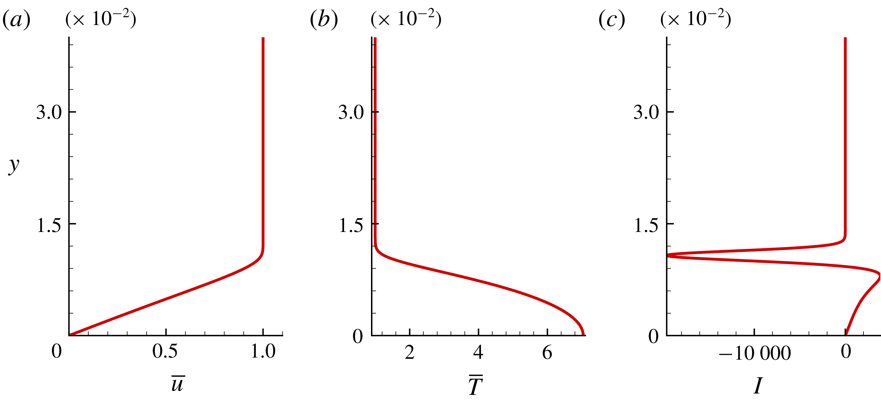
) stations where the first and second modes are respectively dominant, with particular emphasis on the vicinity of the FS synchronization location. Representative mean flow profiles obtained using the Levy–Lees similarity solution (Anderson Reference Anderson2000) are shown in figure 2 for an adiabatic wall, resulting in a wall temperature,
 $T_{adb}/T_{\infty }\sim 7.04$
, where
 $T_{\infty }$
is the free-stream temperature. The mean streamwise velocity
 $\bar{u}$
, temperature
 $\bar{T}$
and
 $\mathit{I}=(\unicode[STIX]{x2202}/\unicode[STIX]{x2202}y)[(1/\bar{T})(\unicode[STIX]{x2202}\bar{u}/\unicode[STIX]{x2202}y)]$
, used to identify the locations of GIPs, are plotted in figures 2(a), 2(b) and 2(c), respectively. The profiles in figure 2 correspond to the streamwise location
 $x=0.9$
, where the boundary layer thickness is
 $\unicode[STIX]{x1D6FF}=0.0107$
. As discussed later, peak amplification of Mack-mode instabilities (for the instability-wave parameters considered) is observed in the vicinity of this location. The GIP, corresponding to the zero-crossing of the function
 $\mathit{I}$
in figure 2(c), is at
 $y\sim 0.0092$
, which is also a region of high mean flow gradients: its existence is a necessary condition for inviscid instability of a compressible boundary layer (Lees & Lin Reference Lees and Lin1946).
Mean flow similarity solution, plotted at
 $x=0.9$
. (a) Mean streamwise velocity,
 $\bar{u}$
, (b) mean temperature,
 $\bar{T}$
, and (c) profile of
 $\mathit{I}=(\unicode[STIX]{x2202}/\unicode[STIX]{x2202}y)[(1/\bar{T})(\unicode[STIX]{x2202}\bar{u}/\unicode[STIX]{x2202}y)]$
.

4 Fluid-thermodynamic decomposition of linear stability theory modes
In the present section, we examine the FT composition of LST-based eigenfunctions in the Mack-mode region. The decomposition provides direct quantitative evaluation of each of the three components, and furthermore yields insight into how each changes in the vicinity of the FS synchronization point.
4.1 Brief description of linear stability theory eigenmodes
The linear instability modes of the underlying base flow are first extracted using a local temporal stability analysis (Malik Reference Malik1990). The linearization of the Navier–Stokes equations is performed using the traditional approach. Denoting a primitive variable as
 $\unicode[STIX]{x1D719}$
:
 $$\begin{eqnarray}\displaystyle \unicode[STIX]{x1D719}=\bar{\unicode[STIX]{x1D719}}+\unicode[STIX]{x1D719}^{\prime },\quad \unicode[STIX]{x1D719}^{\prime }=\hat{\unicode[STIX]{x1D719}}(y)\text{e}^{\text{i}(\unicode[STIX]{x1D6FC}x+\unicode[STIX]{x1D6FD}z-\unicode[STIX]{x1D714}t)}. & & \displaystyle\end{eqnarray}$$
Time-averaged and perturbation quantities are represented by
 $\bar{(\cdot )}$
and
 $(\cdot )^{\prime }$
, respectively,
 $\unicode[STIX]{x1D6FC}$
and
 $\unicode[STIX]{x1D6FD}$
are the streamwise and spanwise wavenumbers, and
 $\unicode[STIX]{x1D714}$
is the circular frequency. In the current temporal analysis, the wavenumbers are real and frequencies are complex numbers. Since the two-dimensional form of second-mode (or Mack-mode) instabilities is often found to amplify the most (Malik Reference Malik1990; Yao et al.
Reference Yao, Krishnan, Sandham and Roberts2007), we focus on
 $\unicode[STIX]{x1D6FD}=0$
for the cases described here. In the eigenvalue problem, all perturbations are assumed to vanish at the free-stream boundary. On the plate surface, velocity and temperature perturbations are zero, and the Neumann condition is applied on pressure perturbations.
The second mode, being the most unstable wave at the conditions of interest, is analysed first. Based on the DNS results to be discussed later, the peak amplitude of a representative second mode with a wavelength
 $\unicode[STIX]{x1D706}\sim 0.025$
is observed at
 $x\sim 0.9$
. Thus, in this temporal stability analysis, we choose the profile at
 $x=0.9$
, shown in figure 2, and obtain the global spectrum (complex circular frequency) for the wavenumber,
 $\unicode[STIX]{x1D6FC}=2\unicode[STIX]{x03C0}/\unicode[STIX]{x1D706}$
, corresponding to
 $\unicode[STIX]{x1D706}=0.025$
. The unstable second mode at this configuration occurs at a frequency of
 $\unicode[STIX]{x1D714}_{r}\sim 232$
(real part) and an amplification rate of
 $\unicode[STIX]{x1D714}_{i}\sim 4.16$
(imaginary part). The corresponding phase speed of this wave is given by
 $c=\unicode[STIX]{x1D714}_{r}/\unicode[STIX]{x1D6FC}\sim 0.924$
, which lies closer to the lower value in the range
 $(1-1/M_{\infty })\sim 0.834$
and
 $(1+1/M_{\infty })\sim 1.167$
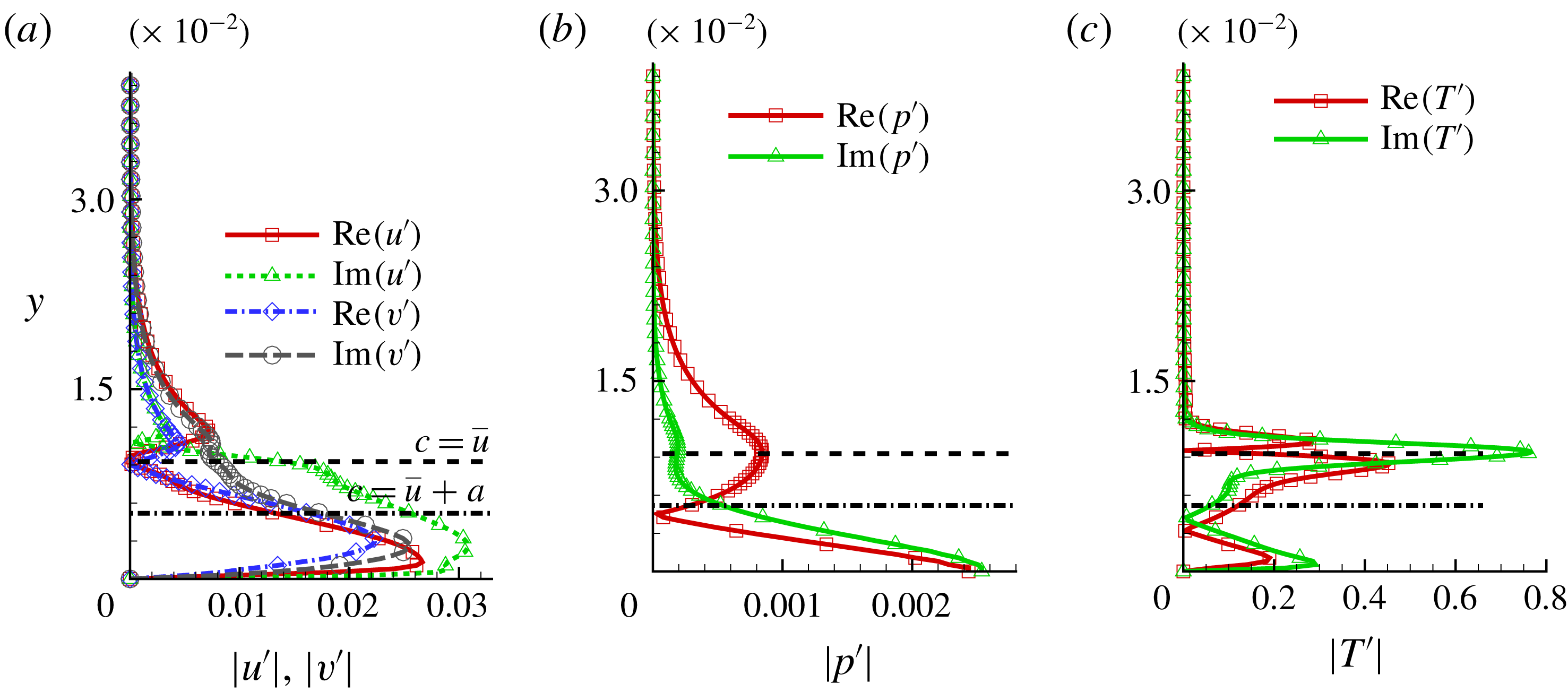
. Figures 3(a), 3(b) and 3(c) plot the real and imaginary parts of perturbation velocities, pressure and temperature eigenfunctions, respectively. The sonic line (where the phase speed of the disturbance is locally sonic with respect to the base flow) represented by
 $c=\bar{u}+a$
(dash-dotted line) and the critical layer where
 $c=\bar{u}$
(dashed line) are also marked. As noted earlier in figure 2(b), the mean temperature variation across the boundary layer exceeds a factor of seven. Thus, in such high-Mach-number mean flows, the magnitudes of temperature perturbation eigenfunctions are typically observed to be significantly higher than those in velocity components (Erlebacher & Hussaini Reference Erlebacher and Hussaini1990). This observation holds in the present case, consistent with prior observations in HBL calculations (Malik Reference Malik1990). The temperature perturbations peak near the GIP at
 $y\sim 0.0092$
, which is observed to be very close to the critical layer (and hence not marked separately). Since the phase speed of this wave is greater than
 $(1-1/M_{\infty })$
, there exists only one sonic line (Bitter & Shepherd Reference Bitter and Shepherd2015). The perturbations are supersonic with respect to the mean flow in the region bounded by this line and the plate surface, and subsonic above it. The pressure perturbations indicate a zero-crossing near this sonic line (figure 3
b). Hence, the second mode does not contribute to significant radiation outside the boundary layer, and decays asymptotically (Bitter & Shepherd Reference Bitter and Shepherd2015) in the current configuration.
Real (Re) and imaginary (Im) parts of unstable second-mode eigenfunctions: (a) velocity, (b) pressure and (c) temperature. Absolute values of corresponding eigenfunctions are plotted. The sonic line and the critical layer are marked using a dash-dotted and dashed line, respectively.

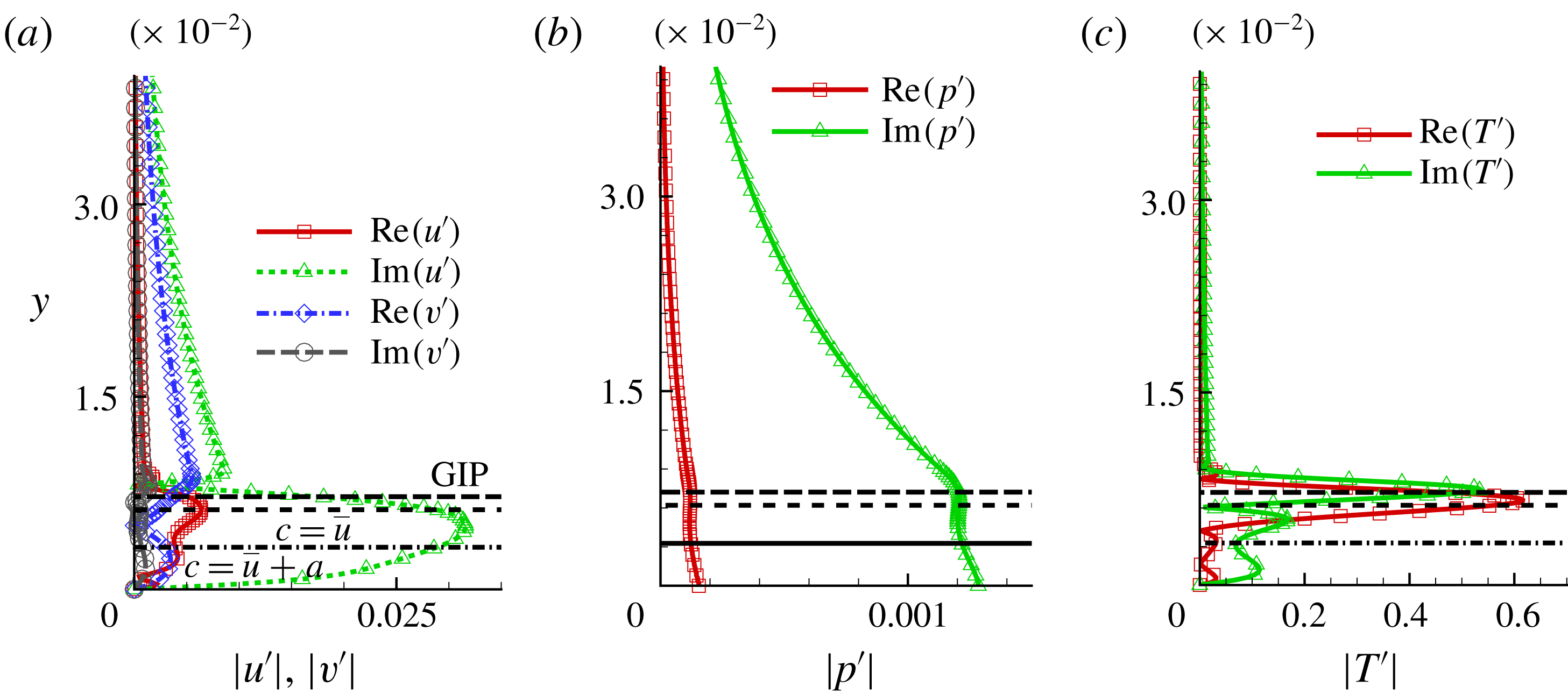
For completeness, we also comment below on the FT composition of first-mode instabilities, even though they are not the dominant form of instability in the Mach regime under consideration. Temporal analysis of the instability eigenspectrum shows first-mode instabilities comprising relatively lower wavenumbers. Following Özgen & Kırcalı (Reference Özgen and Kırcalı2008), we choose a representative wave of
 $\unicode[STIX]{x1D706}=0.075$
, which exhibits first-mode instability at
 $x\sim 0.5$
. The corresponding circular frequency of this wave is
 $\unicode[STIX]{x1D714}_{r}\sim 72.9$
, and it travels at a phase speed of
 $c\sim 0.87$
. The eigenfunctions of this instability wave are plotted in figure 4. In addition to the sonic and critical layers, the GIP, which occurs at
 $y\sim 0.0072$
, is also marked. Similar to the second-mode results of figure 3, the velocity perturbations peak within the boundary layer and their magnitudes are smaller than temperature perturbations. The temperature eigenfunctions also show peak values in the vicinity of the GIP. However, unlike the second-mode instability, the first-mode pressure eigenfunctions do not contain a zero-crossing near the sonic line, consistent with the theory of Mack (Reference Mack1984), where an
 $n$
th-mode pressure eigenfunction is observed to possess
 $(n-1)$
zero-crossings.
Real (Re) and imaginary (Im) parts of unstable first-mode eigenfunctions: (a) velocity, (b) pressure and (c) temperature. Absolute values of corresponding eigenfunctions are plotted. The sonic line and the critical layer are marked using a dash-dotted and dashed line, respectively. The long-dashed line represents the location of GIP.

4.2 Fluid-thermodynamic components of linear stability theory eigenmodes
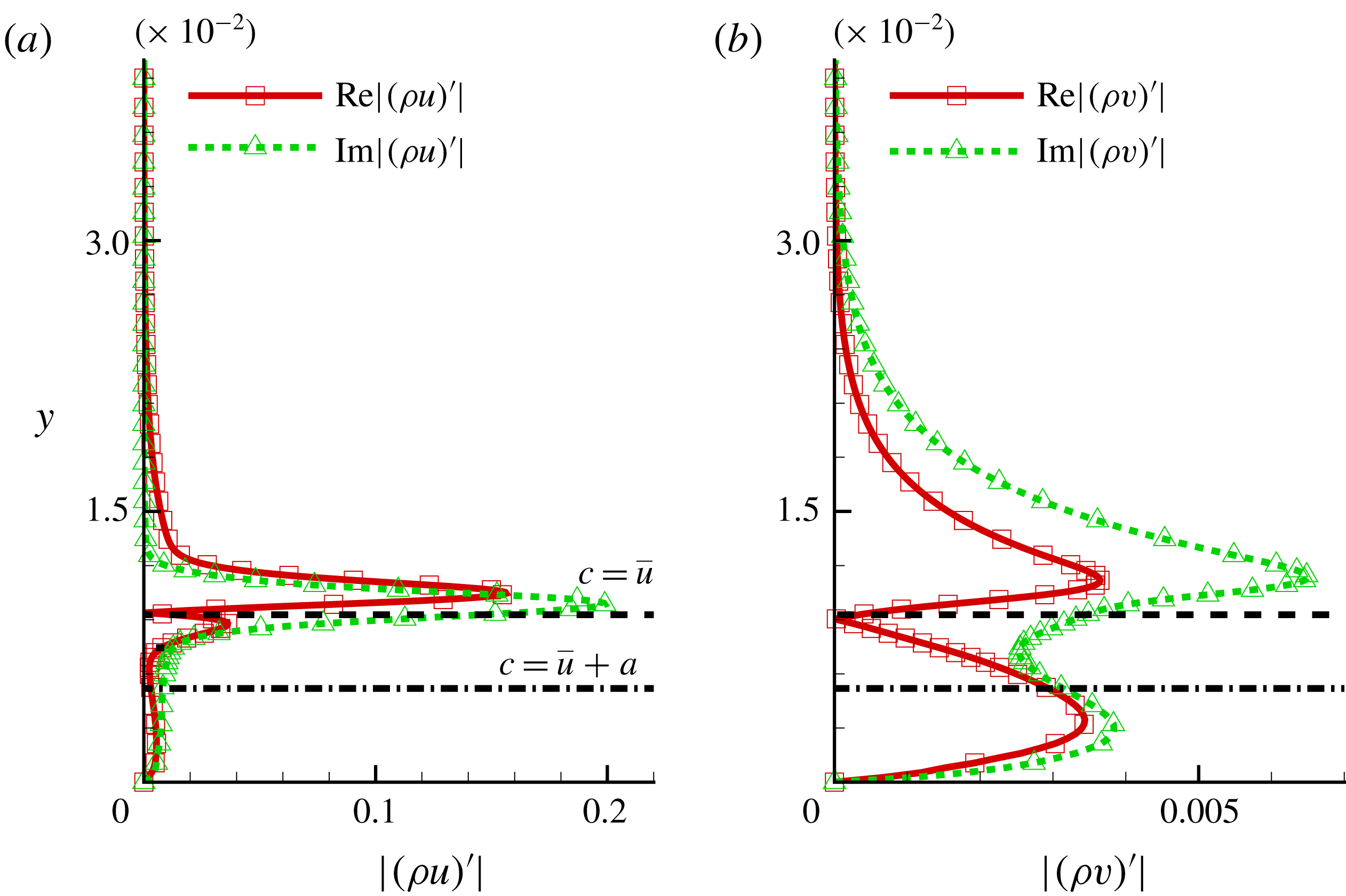
Real (Re) and imaginary (Im) parts of total momentum fluctuations associated with the second mode: (a) streamwise momentum fluctuations and (b) wall-normal momentum fluctuations. Absolute values of corresponding profiles are plotted. The sonic line and the critical layer are marked using a dash-dotted and dashed line, respectively.

The FT decomposition process described in § 2 simplifies greatly under the parallel-flow approximation employed for LST. For reference, the magnitudes of momentum fluctuations,
 $(\unicode[STIX]{x1D70C}u)^{\prime }$
and
 $(\unicode[STIX]{x1D70C}v)^{\prime }$
, associated with the second mode shown in figure 3, are plotted in figure 5. The linearization procedure on total momentum fluctuations yields
 $$\begin{eqnarray}\displaystyle (\unicode[STIX]{x1D70C}u)^{\prime }=\bar{\unicode[STIX]{x1D70C}}u^{\prime }+\bar{u}\unicode[STIX]{x1D70C}^{\prime },\quad (\unicode[STIX]{x1D70C}v)^{\prime }=\bar{\unicode[STIX]{x1D70C}}v^{\prime }+\bar{v}\unicode[STIX]{x1D70C}^{\prime }. & & \displaystyle\end{eqnarray}$$
Using the harmonic ansatz for pressure perturbations as in (4.1) (considering only
 $\unicode[STIX]{x1D6FD}=0$
), the Poisson equation for the acoustic component (2.4) is written as
 $$\begin{eqnarray}\displaystyle \unicode[STIX]{x1D6FB}^{2}\unicode[STIX]{x1D713}_{A}^{\prime }=\frac{1}{\bar{a}^{2}}[-\text{i}\unicode[STIX]{x1D714}\hat{P}(y)\text{e}^{\text{i}(\unicode[STIX]{x1D6FC}x-\unicode[STIX]{x1D714}t)}], & & \displaystyle\end{eqnarray}$$
where the unperturbed local sonic velocity,
 $\bar{a}$
, is used for simplicity. Assuming a similar ansatz for
 $\unicode[STIX]{x1D713}_{A}^{\prime }$
:
 $$\begin{eqnarray}\displaystyle & \displaystyle -\unicode[STIX]{x1D6FC}^{2}\hat{\unicode[STIX]{x1D713}_{A}^{\prime }}(y)\text{e}^{\text{i}(\unicode[STIX]{x1D6FC}x-\unicode[STIX]{x1D714}t)}+\frac{\unicode[STIX]{x2202}^{2}\hat{\unicode[STIX]{x1D713}_{A}^{\prime }}(y)}{\unicode[STIX]{x2202}y^{2}}\text{e}^{\text{i}(\unicode[STIX]{x1D6FC}x-\unicode[STIX]{x1D714}t)}=\frac{1}{\bar{a}^{2}}[-\text{i}\unicode[STIX]{x1D714}\hat{P}(y)\text{e}^{\text{i}(\unicode[STIX]{x1D6FC}x-\unicode[STIX]{x1D714}t)}], & \displaystyle\end{eqnarray}$$
 $$\begin{eqnarray}\displaystyle & \displaystyle \frac{\unicode[STIX]{x2202}^{2}\hat{\unicode[STIX]{x1D713}_{A}^{\prime }}(y)}{\unicode[STIX]{x2202}y^{2}}-\unicode[STIX]{x1D6FC}^{2}\hat{\unicode[STIX]{x1D713}_{A}^{\prime }}(y)=-\frac{\text{i}\unicode[STIX]{x1D714}\hat{P}(y)}{\bar{a}^{2}}. & \displaystyle\end{eqnarray}$$
This one-dimensional ordinary differential equation is discretized using a second-order stencil. The tridiagonal system so obtained is solved using the least-squares method, with wall and free-stream boundary conditions corresponding to no-slip and the boundedness constraint, respectively. The scalar potential of the total irrotational field,
 $\unicode[STIX]{x1D713}^{\prime }$
, is also solved in similar manner, using the corresponding source term
 $\unicode[STIX]{x2202}\unicode[STIX]{x1D70C}^{\prime }/\unicode[STIX]{x2202}t$
. Finally, all FT components are separated out, following the procedure described in § 2.
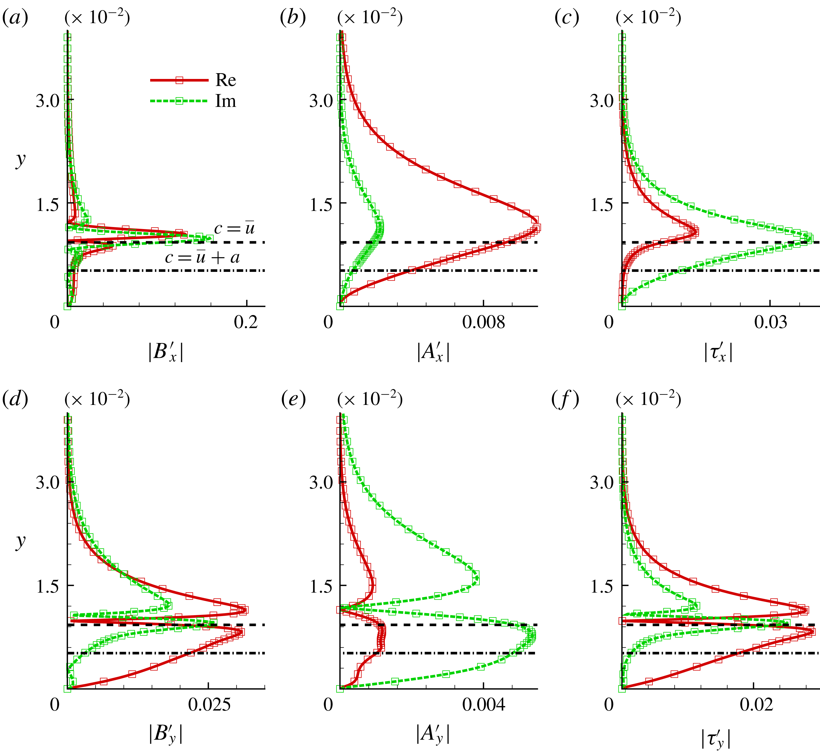
Real and imaginary parts of: (a,d) vortical, (b,e) acoustic and (c,f) thermal perturbations. Absolute values of corresponding profiles are plotted. The top and bottom rows represent the streamwise and wall-normal components, respectively. The sonic line and the critical layer are marked using a dash-dotted and dashed line, respectively. The eigenfunction decomposed corresponds to that of the unstable second mode discussed in figure 3.

The vortical, acoustic and thermal components of the LST eigenfunctions of the unstable second mode of figure 3 are presented in figure 6. For notational convenience, these components are designated
 $\boldsymbol{B}^{\prime }=(B_{x}^{\prime },B_{y}^{\prime })$
,
 $-\unicode[STIX]{x1D735}\unicode[STIX]{x1D713}_{A}^{\prime }=(A_{x}^{\prime },A_{y}^{\prime })$
and
 $-\unicode[STIX]{x1D735}\unicode[STIX]{x1D713}_{T}^{\prime }=(\unicode[STIX]{x1D70F}_{x}^{\prime },\unicode[STIX]{x1D70F}_{y}^{\prime })$
, respectively. Absolute values of the
 $x$
-components are plotted in the top row of figure 6, while the corresponding
 $y$
-components are in the bottom row. In each panel, the solid curve is the real part and the dashed curve denotes the imaginary part. The sonic line and the critical layer are marked using a dash-dotted and dashed line, respectively. The primary observation is that the magnitude of the vortical perturbation component is the largest, followed by the thermal and then acoustic perturbations, respectively. Thus, even after FS synchronization, vortical fluctuations comprise most of the disturbance energy in the Mack modes. As discussed later in this section, this does not imply that it is the most dynamically active component, in terms of changes in its contribution to the eigenfunction of mode S. Peak fluctuations are observed in the vicinity of strong mean flow gradients, i.e. at close proximity to the GIP (figure 6
a). On the other hand, acoustic fluctuations peak slightly above the critical layer (figure 6
b). The location of the peak for the thermal component is similar to that of the vortical component. Figure 6(d,e) also indicates, interestingly, that the wall-normal FT components switch sign just above the GIP (as indicated by the
 $y$
-location where these components are zero). The implication of this observation, and the correspondence with the physical structure of the different FT components, will be discussed later with DNS data (§ 5.1). Finally, we note that, since
 $(\unicode[STIX]{x1D70C}\boldsymbol{u})^{\prime }$
is being decomposed for reasons outlined in § 2, all components go to zero at the wall. This does not imply that vorticity and pressure fluctuations are zero at the wall. The wall vorticity is accounted for in the curl of the solenoidal component, as calculated at the wall. The pressure fluctuations on the wall are dependent on interior values, through the boundary condition.
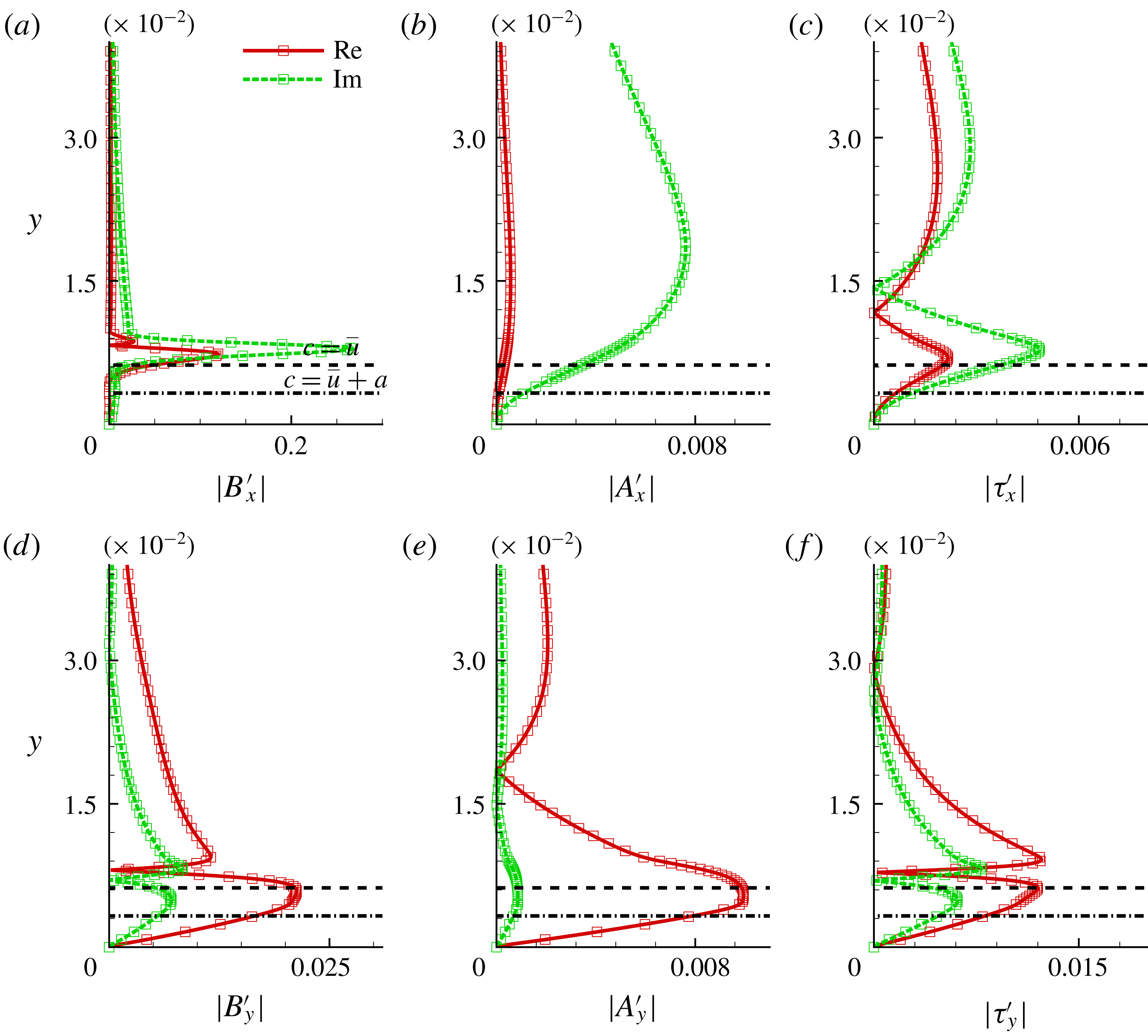
The FT composition of the first mode can also be explored by performing the same operations on the perturbations of figure 4. The results are plotted in figure 7. Comparing figures 6 and 7, it is evident that the vortical content in both the first and second modes are of similar magnitude, with peak values achieved near the GIP. Although the acoustic component appears to be of similar overall magnitude in both cases, it does not possess a zero-crossing in the vicinity of the critical layer in the first mode. This is evident in figure 7(e): this observation is related to key differences in the evolution of first- and second-mode acoustic components, as discussed later. The thermal component, on the other hand, is significantly weaker in the first mode.
Real and imaginary parts of: (a,d) vortical, (b,e) acoustic and (c,f) thermal perturbations. Absolute values of corresponding profiles are plotted. The top and bottom rows represent the streamwise and wall-normal components, respectively. The sonic line and the critical layer are marked using a dash-dotted and dashed line, respectively. The eigenfunction decomposed corresponds to that of the unstable first mode discussed in figure 4.

To understand how the FT components evolve as the boundary layer develops, the above decomposition is performed on a range of locations on the plate. For convenience, we choose the same representative unstable second mode discussed previously, with
 $\unicode[STIX]{x1D706}=0.025$
. To follow the evolution of this unstable mode (mode S) across the first FS synchronization location, which occurs at
 $x\sim 0.7$
(Egorov, Fedorov & Soudakov Reference Egorov, Fedorov and Soudakov2008), the LST eigenspectrum is obtained at locations from
 $x=0.4$
to
 $x=2$
along the streamwise direction. The eigenfunction of mode S and the corresponding mode F with which it first synchronizes are then extracted at each location, and subjected to FT decomposition to understand the evolving redistribution of amplitudes among the three FT components.
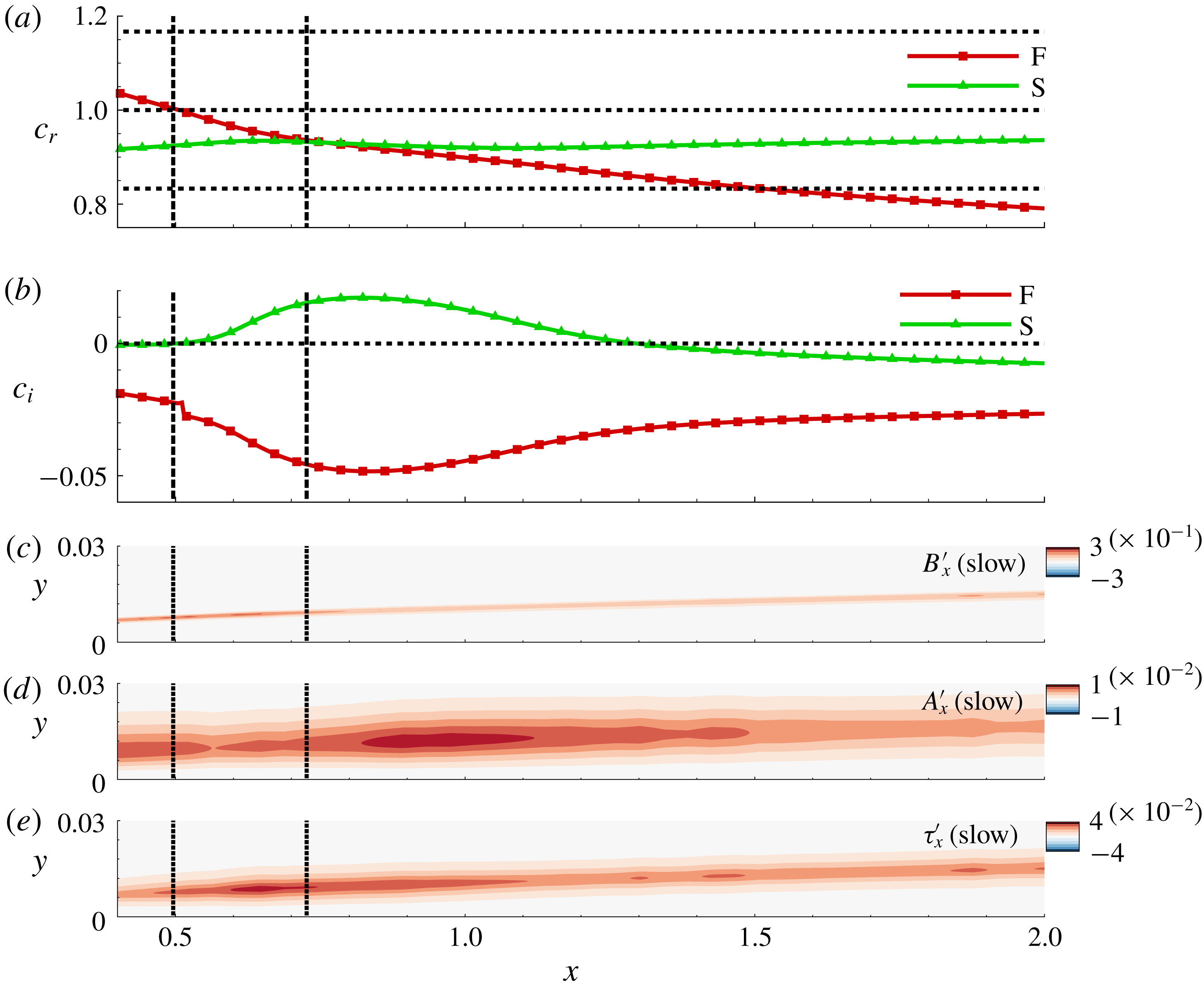
The phase speeds of mode S and mode F are plotted as a function of
 $x$
in figure 8(a). As expected, the phase speed of mode F decreases from
 $(1+1/M_{\infty })$
near the leading edge of the plate as the wave propagates downstream. Mode S gradually increases in phase speed and eventually synchronizes with mode F at
 $x\sim 0.7$
. These results are qualitatively consistent with the summary description in Fedorov (Reference Fedorov2011) and Zhong & Wang (Reference Zhong and Wang2012). Further downstream, the phase speed of mode F decreases below
 $(1-1/M_{\infty })$
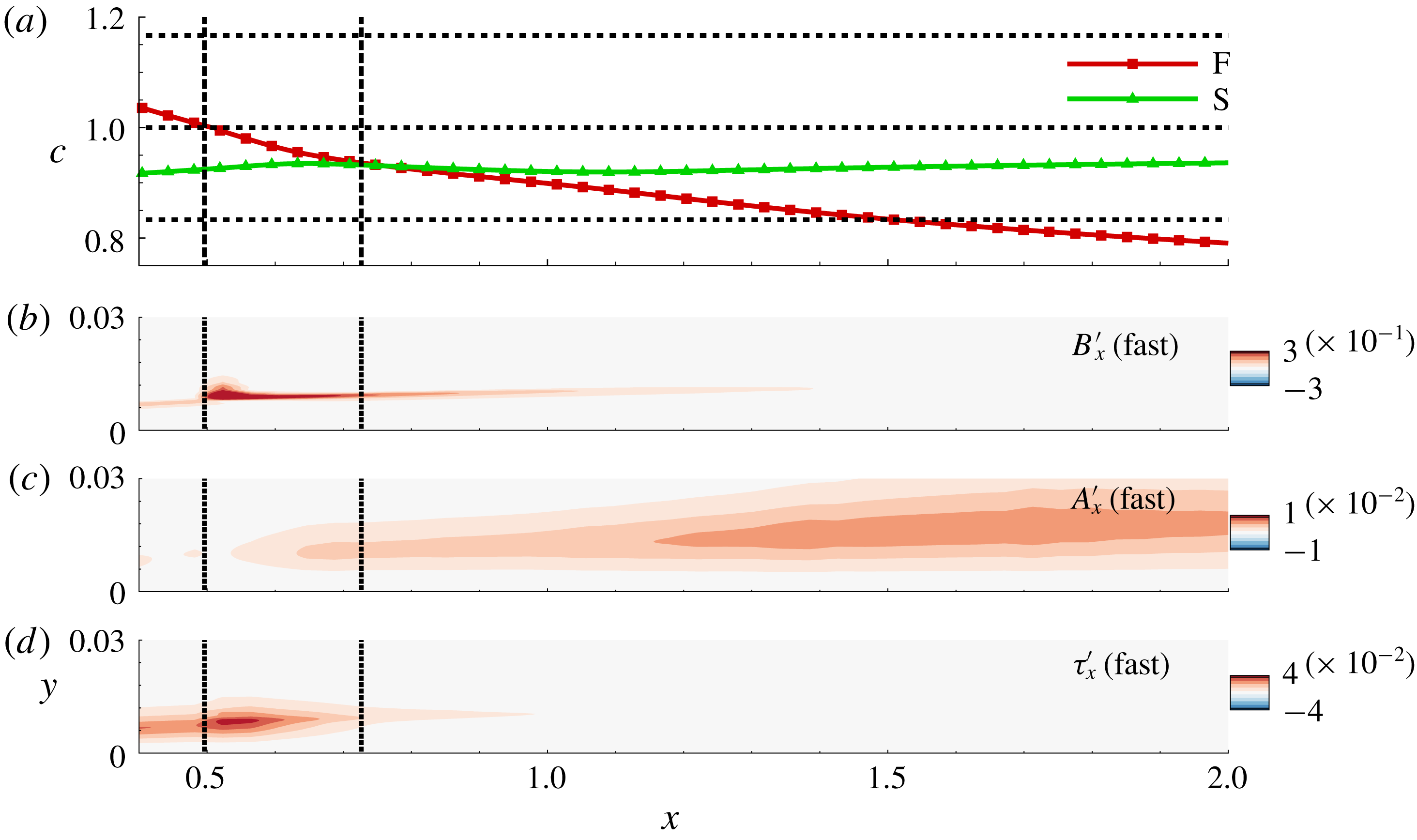
, whereas that of mode S nearly levels off at a value slightly below unity. For further reference, the two locations where mode F first achieves a phase speed of unity and subsequently that of mode S are marked by two vertical dotted lines. The amplification rates of these modes are plotted in figure 8(b). It is evident that in the post-synchronization region, mode S achieves peak amplification, as indicated by its high positive values.
Adiabatic wall results. (a) Variation of phase speeds of mode S and mode F across the FS synchronization point. (b) Variation of amplification rate of mode S and mode F across the FS synchronization point. Variation of the (c) vortical, (d) acoustic and (e) thermal content in mode S during FS synchronization. The two vertical dotted lines in each panel mark the approximate location where mode F attains a phase speed of unity and where it synchronizes with mode S, respectively.

Since the interest is in the most amplified instability wave, we first analyse the FT amplitudes in mode S in figures 8(c), 8(d) and 8(e), using the real parts of streamwise components of the vortical, acoustic and thermal perturbations, respectively. Consistent with the earlier observation made in the context of figure 6, the peaks in the vortical and thermal components closely follow the highest gradients in the boundary layer near the GIP. The acoustic component, however, displays peak values slightly above this location. The vortical content remains the largest FT component amplitude at all locations examined (note the different ranges employed). Also, the vortical component contains no apparent feature that might indicate a signature of the synchronization procedure.
Figure 8(d), however, clearly displays a change in shape of the eigenfunction. This is consistent with increased acoustic component content near the FS synchronization location, with a local peak in the range
 $0.6<x<1.6$
, and a maximum value at
 $x\sim 0.9$
, where the Mack mode is observed to be most amplified. Thus, even though the acoustic component is the smallest of the three, it is the most dynamically active in the post-synchronization region. Thermal perturbations also manifest changes near the FS synchronization point, albeit less dramatically so than the acoustic components (figure 8
e). However, both thermal and acoustic components show rapid changes upstream of the synchronization point, (
 $x\sim 0.625$
). Although not included here for brevity, based on analyses encompassing a wide range of hypersonic Mach numbers (
 $4\leqslant M_{\infty }\leqslant 8$
), it is observed that mode S consistently displays an acoustic gain during its evolution in the second neutral curve, preceded by a corresponding thermal gain in its eigenfunction.
The corresponding FT components of mode F are plotted in figure 9. Again, the phase speeds of mode S and mode F are reproduced in figure 9(a) for reference, and the two locations where mode F matches the phase speed of unity and that of mode S are also marked. The most significant difference in the evolution of the FT component of mode F is visible in the vortical content (figure 9
b). When the phase speed equals unity, a sharp localized peak is observed in the vortical content of mode F, as it synchronizes with the vorticity spectrum of the basic state. A similar peak is also observed in the thermal component (figure 9
d), since this phase speed also corresponds to the entropy spectrum (Wang et al.
Reference Wang, Zhong and Ma2011). The observed peaks are, however, limited in their streamwise extent and disappear once mode F moves away from
 $c=1$
. This intersection does not induce any significant change in the acoustic content shown in figure 9(c). The events near this inter-modal synchronization point, i.e. where mode F engages the vorticity and entropy spectra, have been discussed by Fedorov & Tumin (Reference Fedorov and Tumin2003).
Adiabatic wall results. (a) Variation of phase speeds of mode S and mode F across the FS synchronization point. Variation of the (b) vortical, (c) acoustic and (d) thermal content in mode F during FS synchronization. The two vertical dotted lines in each panel mark the approximate location where mode F attains a phase speed of unity and where it synchronizes with mode S, respectively.

The acoustic component in mode F is considerably more affected near the FS synchronization point downstream. However, the resulting amplification here is far less than was observed in mode S (see figure 8). Thus, the FS synchronization channels energy into the acoustic component in both mode S and mode F instability waves at their synchronization point, but to a varying extent. Considering that the vortical content is actually higher in mode F at the FS synchronization point (compare figures 8 c and 9 b), it is the net acoustic gain that determines the further amplification of these modes, and differentiates the wave that will eventually become the most unstable. Effectively, the acoustic contributions to the F and S eigenmodes are qualitatively different at the FS synchronization location. Based on simulations of adiabatic and cold walls, we consistently observe that the acoustic gain is considerably higher for that mode which enters into the second neutral curve, essentially identifying the nature of the second or Mack mode. These results suggest that the dynamics related to Mack-mode amplification involves rapid changes of the thermal and acoustic components.
5 Direct numerical simulations
The linear theory above, establishing the general correspondence between stability and FT components, is limited in fidelity by parallel-flow simplifications and the assumption of a similarity profile. A more realistic assessment may be obtained through DNS, whose accuracy is not inhibited in this manner. In this section, we thus use DNS to explore FT dynamics, including the nonlinear saturation process and the effects of wall thermal conditions.
5.1 Description of direct numerical simulations and validation
To simplify validation, the configuration discussed in Egorov et al. (Reference Egorov, Fedorov and Soudakov2006) and Soudakov et al. (Reference Soudakov, Egorov, Fedorov and Novikov2016) is chosen. The two-dimensional, unsteady Navier–Stokes equations are solved in curvilinear coordinates. The numerical technique includes a third-order upwind-biased reconstruction and Roe scheme (Roe Reference Roe1981) for calculating inviscid fluxes, along with an entropy fix as suggested in Egorov et al. (Reference Egorov, Fedorov and Soudakov2006). The van Leer harmonic limiter (van Leer Reference van Leer1979) is applied to eliminate grid-scale oscillations, and viscous fluxes are discretized using second-order central differences. The nonlinearly stable third-order Runge–Kutta scheme (Shu & Osher Reference Shu and Osher1988) is used for time integration.
The simulation parameters for the DNS calculations are as follows. Non-dimensionalization is achieved using free-stream conditions, which provide velocity (
 $U_{\infty }^{\ast }$
), density (
 $\unicode[STIX]{x1D70C}_{\infty }^{\ast }$
) and temperature (
 $T_{\infty }^{\ast }$
) scales. The streamwise extent of the plate is
 $2L^{\ast }$
, where
 $L^{\ast }$
is the reference length scale, as introduced in § 3. Pressure
 $p^{\ast }$
is normalized using
 $\unicode[STIX]{x1D70C}_{\infty }^{\ast }U_{\infty }^{\ast 2}$
. All calculations are performed at a free-stream Reynolds number of
 $Re=\unicode[STIX]{x1D70C}_{\infty }^{\ast }U_{\infty }^{\ast }L^{\ast }/\unicode[STIX]{x1D707}_{\infty }^{\ast }=2\times 10^{6}$
, where
 $\unicode[STIX]{x1D707}_{\infty }^{\ast }$
is the free-stream dynamic viscosity. The ideal gas law,
 $p=\unicode[STIX]{x1D70C}T/(\unicode[STIX]{x1D6FE}M_{\infty }^{2})$
, holds, where
 $\unicode[STIX]{x1D6FE}$
is the ratio of specific heats. The Prandtl number
 $Pr$
is assumed to be fixed at 0.72 and the temperature dependence of viscosity is modelled as
 $\unicode[STIX]{x1D707}^{\ast }/\unicode[STIX]{x1D707}_{\infty }^{\ast }=(T^{\ast }/T_{\infty }^{\ast })^{0.7}$
.
The rectangular computational region extends over
 $0\leqslant x\leqslant 2$
and
 $0\leqslant y\leqslant 0.47$
, where
 $x=0$
corresponds to the leading edge of the plate, and is resolved with 3021 and 541 nodes in the streamwise and wall-normal directions, respectively. The grid is clustered to resolve the high gradients near the leading edge and the plate surface. A buffer zone damps perturbations near the outer and downstream boundaries. Free-stream conditions are imposed along the inlet and outer boundaries, and a linear interpolation is used to obtain the variables on the outflow boundary. Wall boundary conditions include no slip for the velocity components and zero normal pressure gradient. In the present section, as for the LST, we assume an adiabatic condition, i.e. zero temperature gradient at the wall, while calculating the unperturbed basic state, deferring the cold wall discussion for later.
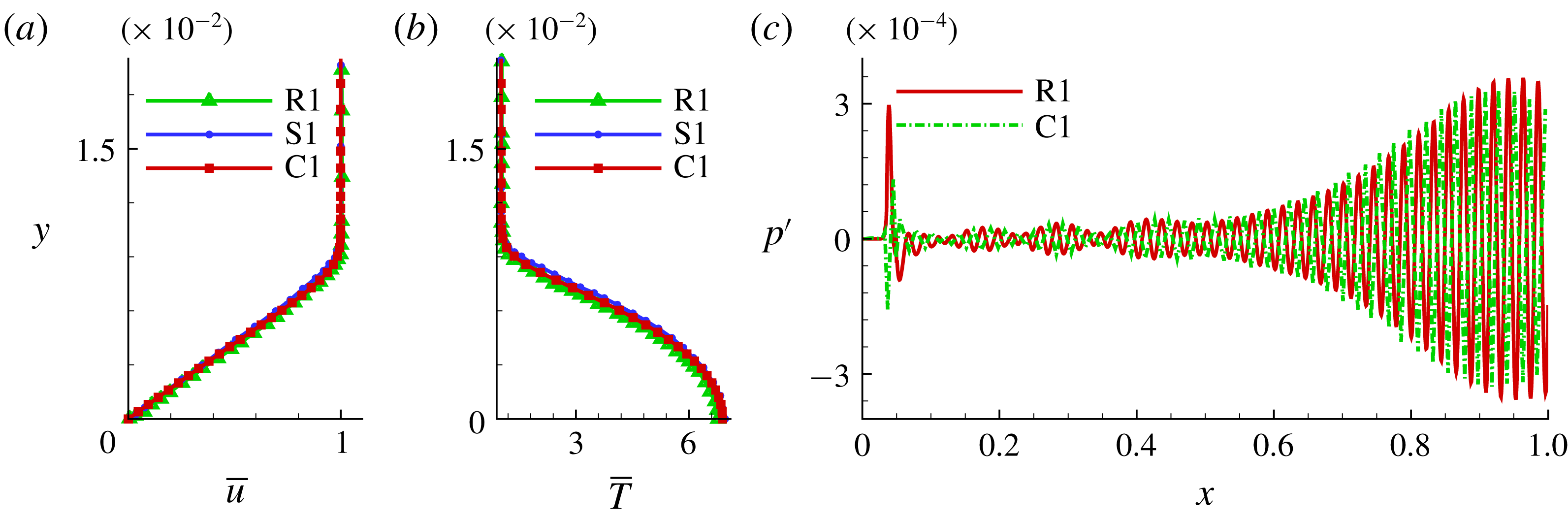
The validation of DNS calculations for the baseline adiabatic case is summarized in figure 10. The streamwise velocity profile at
 $x=0.7$
is shown in figure 10(a). The profiles include the current DNS (C1), the reference simulation (R1) of Egorov et al. (Reference Egorov, Fedorov and Soudakov2006) and the similarity profile (S1). The agreement among the different plots is evident. The corresponding temperature profiles in figure 10(b) also display similar agreement.
(a) Mean streamwise velocity profile at
 $x=0.7$
; R1 is the profile from the reference simulation, S1 is the similarity profile and C1 corresponds to the current computation. (b) Mean temperature profile at
 $x=0.7$
. (c) Perturbation pressure profile obtained on the plate surface.

5.2 Forced direct numerical simulations
We use a simulated wall blowing–suction actuator to initiate second-mode instabilities in the HBL. This procedure usually results in the amplification of mode S, if the actuator is placed upstream of the corresponding synchronization point (Zhong Reference Zhong2001; Wang & Zhong Reference Wang and Zhong2009). The specific form of the wall blowing–suction technique is taken from Egorov et al. (Reference Egorov, Fedorov and Soudakov2006) and Soudakov et al. (Reference Soudakov, Egorov, Fedorov and Novikov2016), where a theoretical actuator is considered, to enforce a sinusoidal wall-normal momentum flux of the following form:
 $$\begin{eqnarray}\displaystyle q_{w}(x,t)=\frac{\unicode[STIX]{x1D70C}_{w}^{\ast }v_{w}^{\ast }}{\unicode[STIX]{x1D70C}_{\infty }^{\ast }U_{\infty }^{\ast }}=A\sin \left(2\unicode[STIX]{x03C0}\frac{x-x_{1}}{x_{2}-x_{1}}\right)\sin (\unicode[STIX]{x1D714}t). & & \displaystyle\end{eqnarray}$$
The value of
 $\unicode[STIX]{x1D714}=\unicode[STIX]{x1D714}^{\ast }L^{\ast }/U_{\infty }^{\ast }$
is chosen to be
 $260$
, where
 $\unicode[STIX]{x1D714}^{\ast }$
is the dimensional circular frequency with non-dimensional frequency parameter
 $F=\unicode[STIX]{x1D714}/R=1.3\times 10^{-4}$
resulting in peak amplification of the second mode at
 $x\sim 0.9$
. The effects of nonlinearity are controlled using the amplitude parameter
 $A$
. For the linear case considered in this section, this value is chosen to be
 $6\times 10^{-4}$
: it is increased to
 $3.6\times 10^{-2}$
for the nonlinear response studied in § 5.6. The forcing is confined to the vicinity of the leading edge of the plate, bounded by
 $x_{1}=0.0358$
and
 $x_{2}=0.0495$
, respectively.
To validate the forced simulation, we compare the wall distribution of fluctuation pressure (
 $p^{\prime }$
), i.e. the difference between the instantaneous forced simulation and the steady basic state, to the reference simulation of Soudakov et al. (Reference Soudakov, Egorov, Fedorov and Novikov2016) at the same forcing parameters. This result, shown in figure 10(c), indicates that the fluctuation evolution is captured accurately. The peak near the leading edge of the plate is the signature of the actuator. The major growth in amplitude observed for
 $x>0.7$
corresponds to second-mode amplification in the HBL. The steady and forced responses are thus suitable to examine the dynamics in terms of FT components.
5.3 Fluid-thermodynamic decomposition of the direct numerical simulation fluctuation field
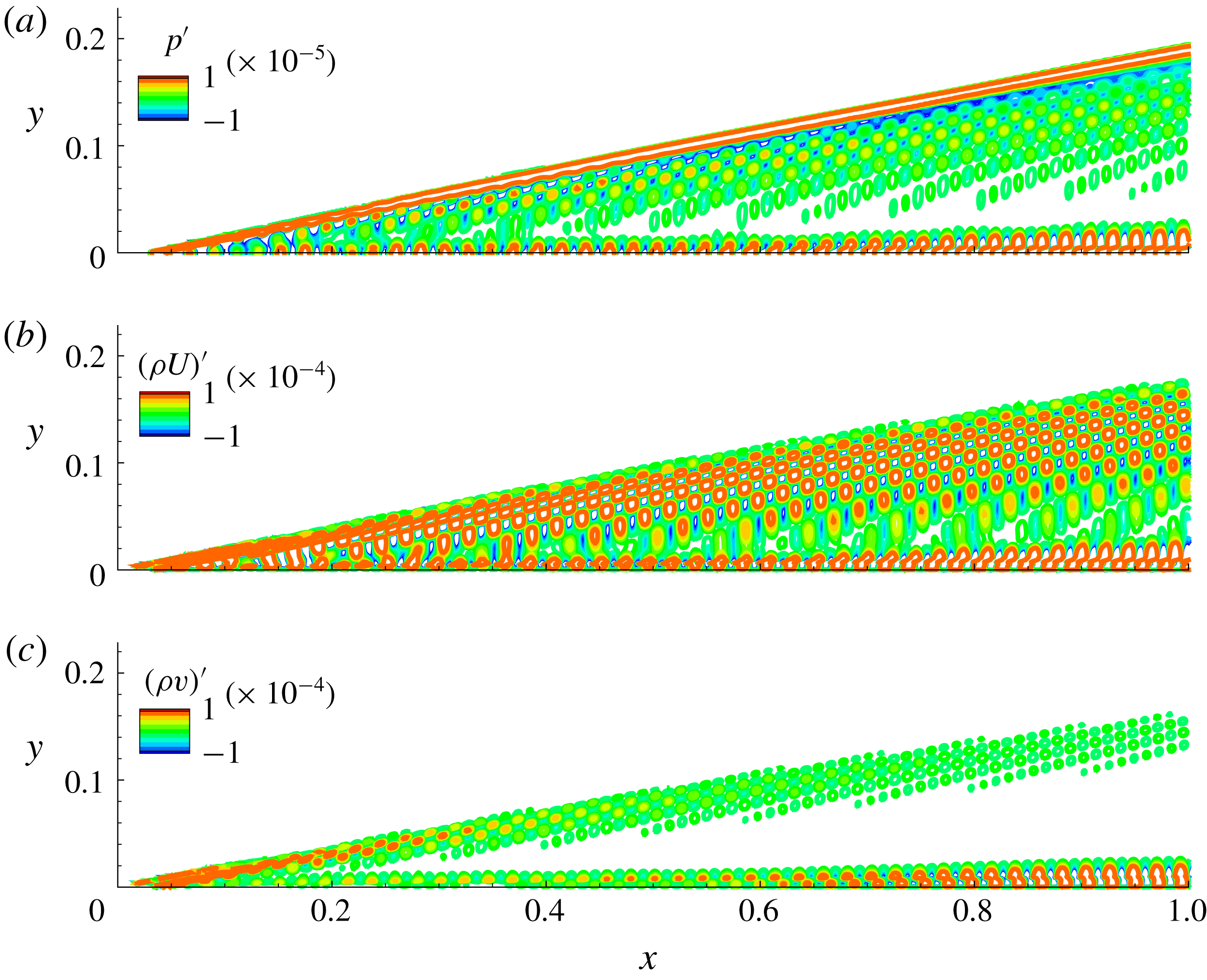
An overall description is provided first, followed by a detailed analysis of the Mack-mode amplification region. Figure 11 shows an instantaneous snapshot of
 $p^{\prime }$
,
 $(\unicode[STIX]{x1D70C}u)^{\prime }$
and
 $(\unicode[STIX]{x1D70C}v)^{\prime }$
fluctuations. The
 $p^{\prime }$
contours in figure 11(a) show fluctuations emanating from the upstream actuator and bifurcating into two regions, one aligning along the shock wave, and the other propagating within the boundary layer. Intermediate streams of acoustic radiation are observed from various streamwise locations in the boundary layer. Fluctuations inside the boundary layer undergo prominent amplification beyond
 $x\sim 0.7$
, which corresponds to the second-mode instability induced by this form of actuation. Contours of the
 $x$
- and
 $y$
-components of momentum density,
 $(\unicode[STIX]{x1D70C}\boldsymbol{u})^{\prime }$
, are also shown in figures 11(b) and 11(c) for reference. In general, the peak values of streamwise momentum fluctuations are an order of magnitude higher than those of the wall-normal component, although both show amplification near the GIP. The radiated component outside the boundary layer is most visible in the streamwise momentum fluctuations, which also display similar spatial form as pressure perturbations in the zone of second-mode amplification.
Instantaneous snapshot of (a) pressure
 $p^{\prime }$
, (b)
 $(\unicode[STIX]{x1D70C}u)^{\prime }$
and (c)
 $(\unicode[STIX]{x1D70C}v)^{\prime }$
.

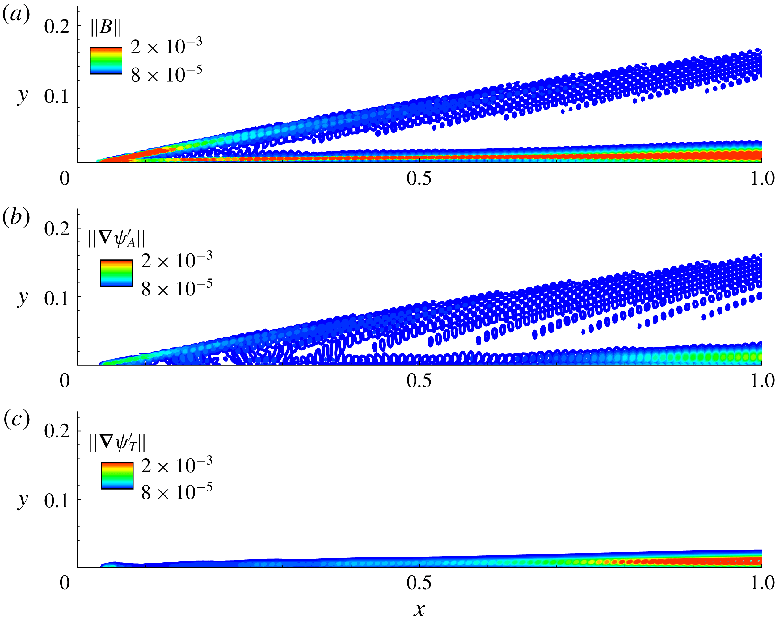
Instantaneous snapshots of the magnitudes of (a) vortical, (b) acoustic and (c) thermal perturbations over the plate surface.

The FT components are extracted by applying the MPT approach of § 2 to the fluctuation field. Figures 12(a), 12(b) and 12(c) depict the magnitudes of the vortical (
 $\Vert \boldsymbol{B}^{\prime }\Vert$
), acoustic (
 $\Vert \unicode[STIX]{x1D735}\unicode[STIX]{x1D713}_{A}^{\prime }\Vert$
) and thermal (
 $\Vert \unicode[STIX]{x1D735}\unicode[STIX]{x1D713}_{T}^{\prime }\Vert$
) components, respectively. Consistent with the LST analysis, the vortical perturbation is the largest in magnitude and captures those from the small fluctuations induced at the leading shock wave by the wall blowing–suction technique. The peak value of
 $\boldsymbol{B}^{\prime }$
consistently occurs near the GIP, where mean flow gradients are large. The acoustic component has a relatively small presence within the boundary layer, until the location of second-mode instability growth, where it amplifies near the critical layer region. Thermal perturbations also have their peak footprint along the locus of the GIP. However, unlike the vortical and acoustic components, which have significant presence outside the boundary layer, the thermal component is more compact, and is restricted to the boundary layer.
The FT decomposition thus highlights the presence of significant vortical perturbations in the second-mode instabilities, even as it also captures the pronounced, dynamically significant role of acoustic waves in the Mack mode. Although not included here, the DNS indicates that Mack-mode amplification leads to a greater rate of growth in the acoustic and thermal component (compared to the hydrodynamic component), when normalized by their respective pre-synchronization values. The radiation streaks from the boundary layer, observed previously in
 $p^{\prime }$
of figure 11, are represented in the acoustic component. These acoustic waves interact with the strong gradients in the shock, and are partly converted into vortical perturbations, as observed near the shock in figure 12(a).
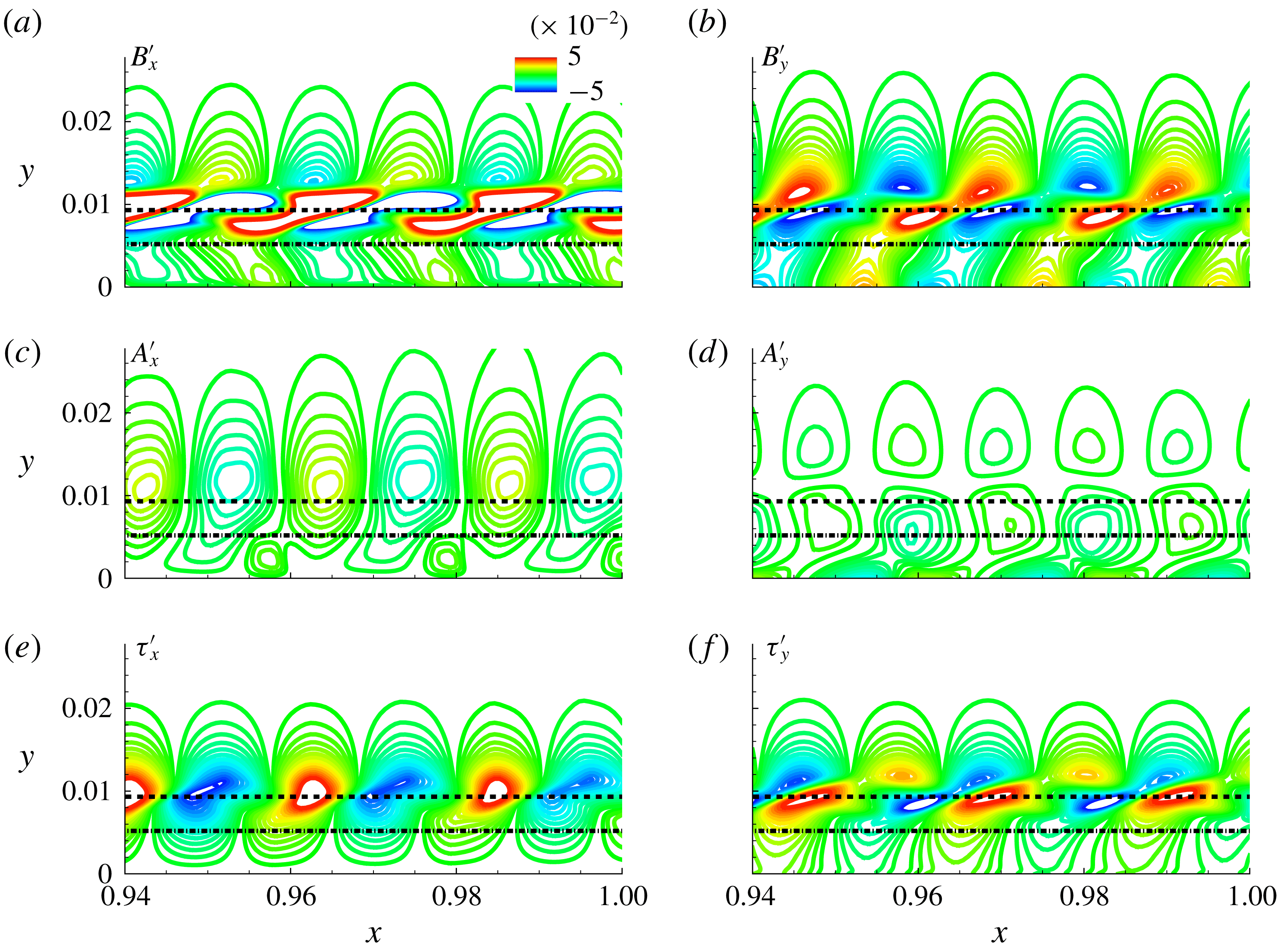
Perturbation structure in the Mack-mode amplification region. Vortical components (a)
 $B_{x}^{\prime }$
and (b)
 $B_{y}^{\prime }$
, acoustic components (c)
 $A_{x}^{\prime }$
and (d)
 $A_{y}^{\prime }$
, and thermal components (e)
 $\unicode[STIX]{x1D70F}_{x}^{\prime }$
and (f)
 $\unicode[STIX]{x1D70F}_{y}^{\prime }$
. The sonic line and the critical layer are marked using a dash-dotted and a dashed line, respectively.

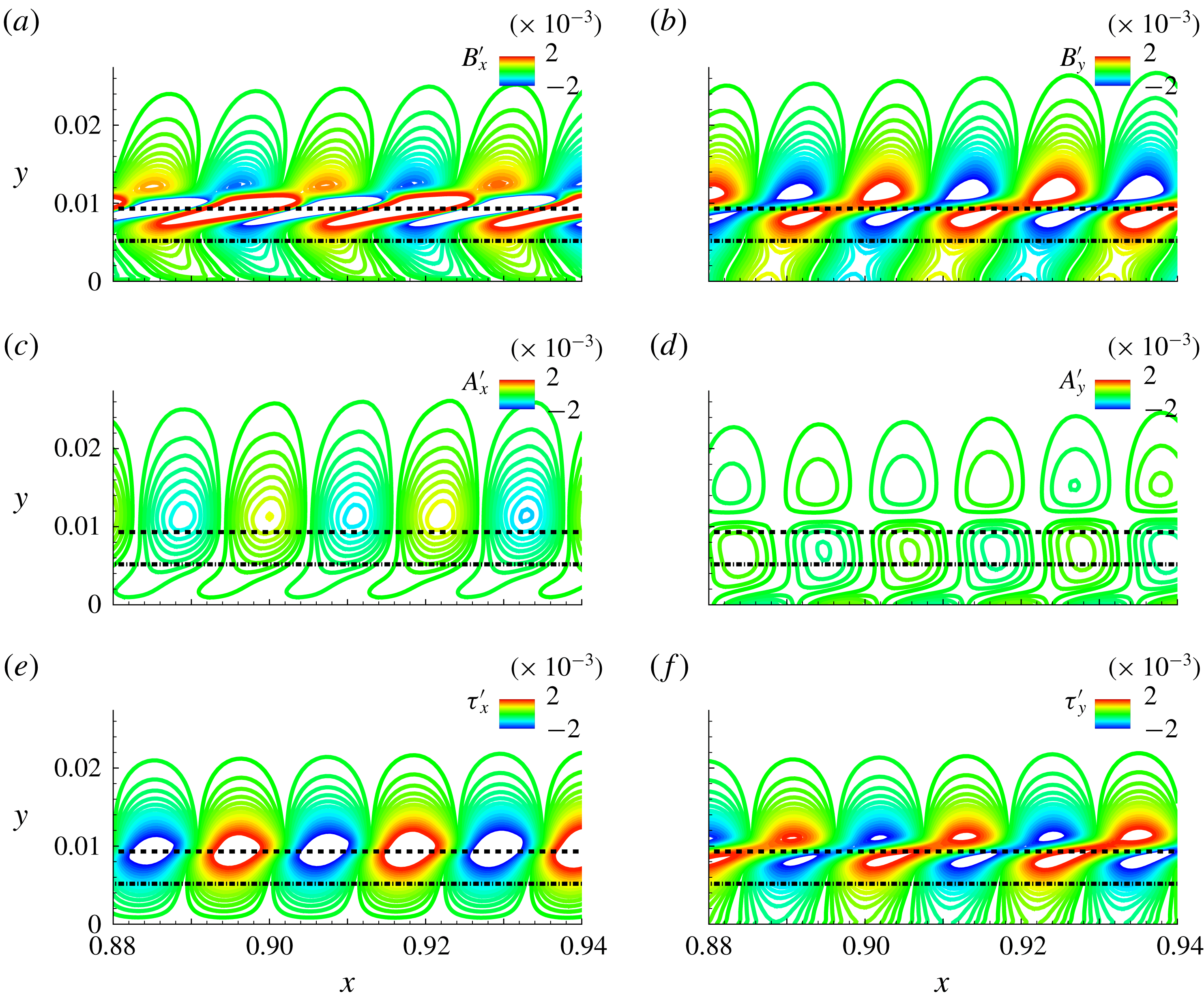
The FT dynamics in the zone of second-mode growth is now explored in detail using a small streamwise region near the FS synchronization location,
 $0.88\leqslant x\leqslant 0.94$
. The profiles of the unsplit momentum fluctuations in the DNS are observed to be consistent with the corresponding LST profiles, plotted in figure 5. The decomposed FT components in this region are shown in figure 13. The
 $x$
- and
 $y$
-components of the vortical (figure 13
a,b), acoustic (figure 13
c,d) and thermal (figure 13
e,f) components are plotted with the same contour range. The dominant amplitude component is again vortical in nature (figure 13
a,b). Peak values, with amplitudes reaching approximately 2 % of the free-stream velocity, straddle the GIP where ‘rope-shaped’ structures, i.e. streamwise elongated and flattened regions of alternating positive and negative peaks, are obtained. Such features have previously been observed in experimental data (Stetson & Kimmel Reference Stetson and Kimmel1993; Laurence, Wagner & Hannemann Reference Laurence, Wagner and Hannemann2016; Kennedy et al.
Reference Kennedy, Laurence, Smith and Marineau2018), as well as numerical simulations (Pruett & Chang Reference Pruett and Chang1995) of Mack-mode growth. The FT analysis thus shows that the primary observable feature in the second-mode amplification zone of the boundary layer is associated with distortions of its vortical content.
The acoustic
 $x$
-component is larger than the
 $y$
-component: both are, however, much smaller than the vortical and thermal perturbations. Peaks are observed above the critical layer in the
 $x$
-component as seen in figure 13(c). The acoustic perturbations in the outer boundary layer lead to intermittent radiation streaks as discussed earlier in figure 12(b). Above the sonic line, the acoustic component and the pressure fluctuations are observed to be in phase and have similar structures. Below the sonic line, however, pressure fluctuations are in phase with the vortical component. Thus, the pressure fluctuations are reflective of different FT components, depending on the location in the boundary layer. This combined vortical and acoustic nature of the pressure field is one cause of the difficulty in using Kovásznay’s approach to decomposing fluctuations into FT components, since it identifies pressure exclusively with the irrotational acoustic field.
The
 $x$
- and
 $y$
-components of thermal perturbations display features common to the other two FT components:
 $\unicode[STIX]{x1D70F}_{y}^{\prime }$
has similar distorted structures to
 $B_{y}^{\prime }$
, while
 $\unicode[STIX]{x1D70F}_{x}^{\prime }$
bears some resemblance to
 $A_{x}^{\prime }$
. The former observation is consistent with the vortical–entropy coupling as suggested by Crocco’s theorem. The explanation of the latter effect is, however, better understood by an examination of the flux lines associated with each component, which are considered next.
Flux lines of the (a) vortical, (b) acoustic and (c) thermal components. In each panel the contours represent the magnitude of the corresponding field.

5.4 Fluxes associated with fluid-thermodynamic components
The vector nature of the momentum density,
 $(\unicode[STIX]{x1D70C}\boldsymbol{u})^{\prime }$
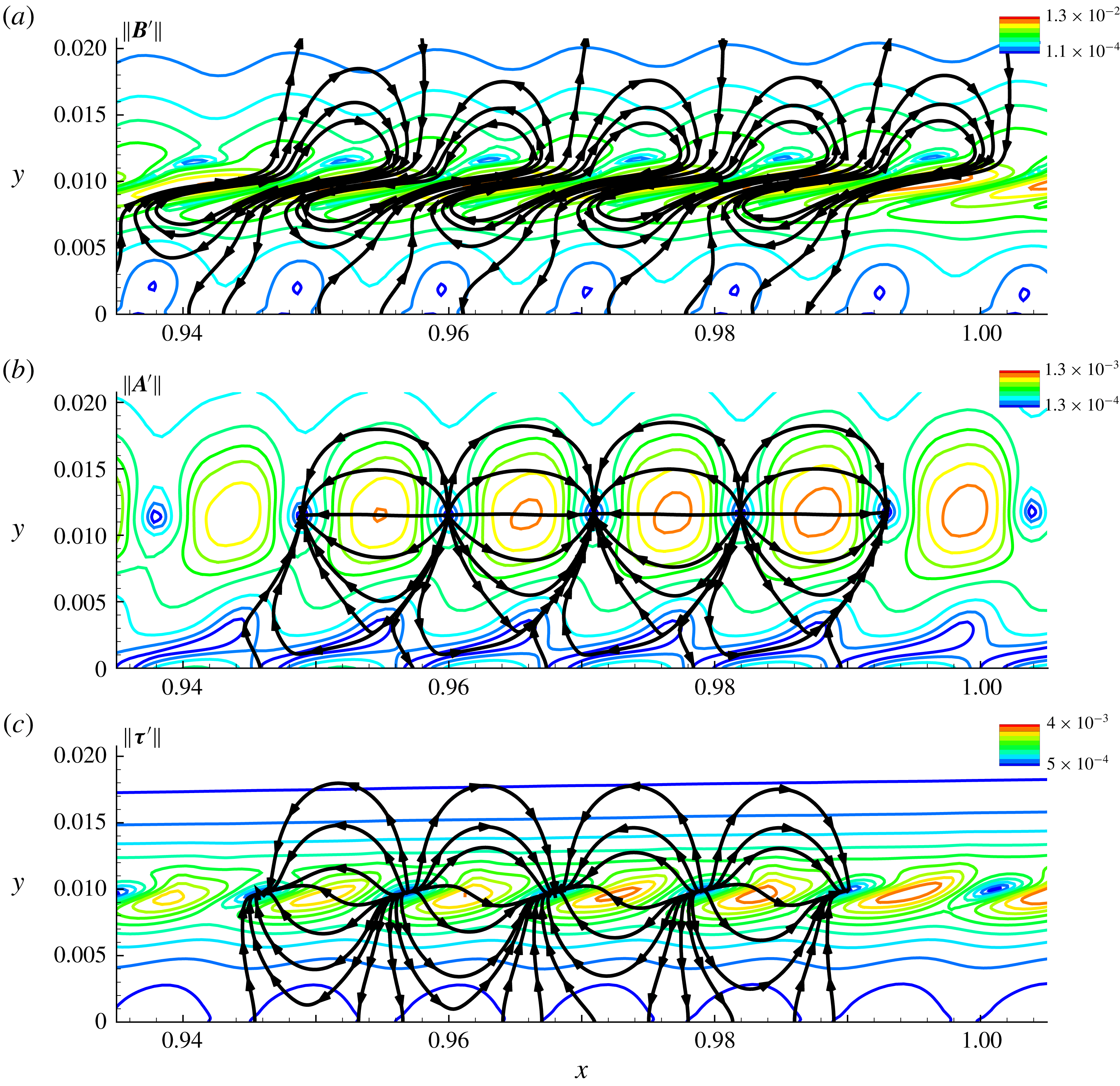
, used to obtain the FT components, facilitates an analysis of the mass fluxes associated with each component. Figure 14(a), (b) and (c) plot the instantaneous flux lines of the vortical, acoustic and thermal components of the Mack mode, using the vector fields
 $(B_{x}^{\prime },B_{y}^{\prime })$
,
 $(A_{x}^{\prime },A_{y}^{\prime })$
and
 $(\unicode[STIX]{x1D70F}_{x}^{\prime },\unicode[STIX]{x1D70F}_{y}^{\prime })$
, respectively. The region of interest spans
 $0.935<x<1.005$
where high perturbation amplitudes are observed. In each panel, the contours represent the magnitude of the corresponding vector field, denoted as
 $\Vert \boldsymbol{B}^{\prime }\Vert$
,
 $\Vert \boldsymbol{A}^{\prime }\Vert$
and
 $\Vert \unicode[STIX]{x1D749}^{\prime }\Vert$
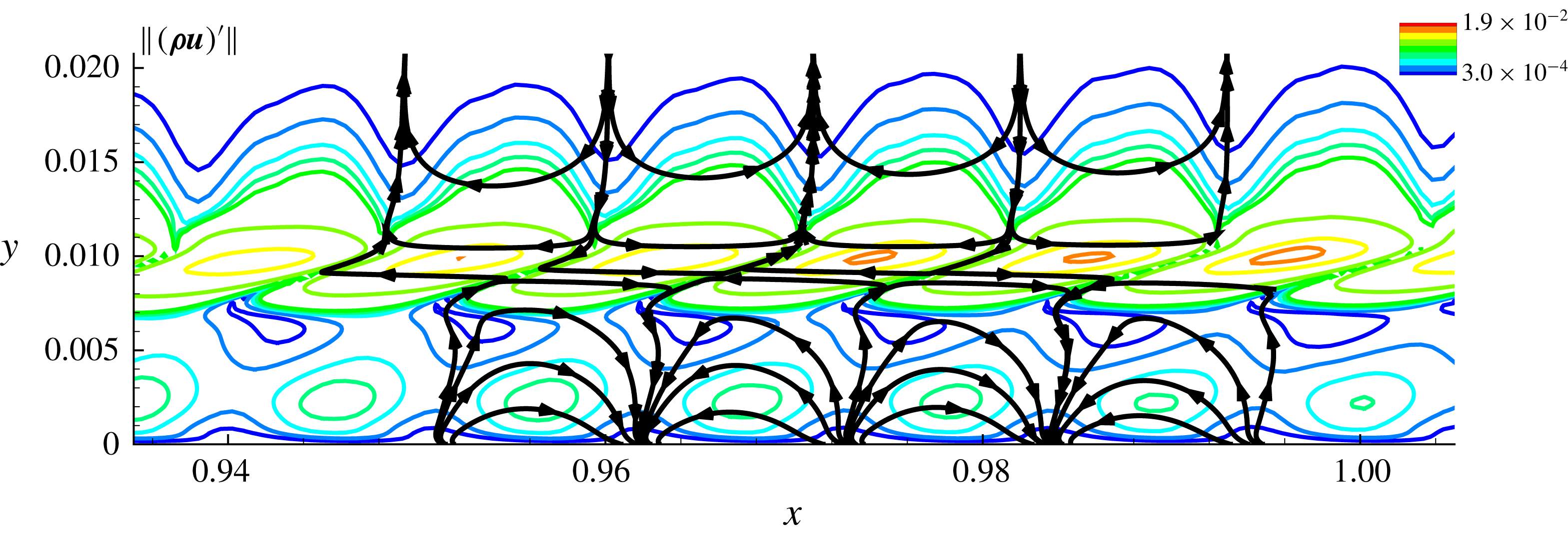
. For reference, the corresponding results for the unsplit
 $\unicode[STIX]{x1D70C}\boldsymbol{u}$
field are shown in figure 15. It is evident from figure 14(a,b) that the vortical and acoustic fields have fundamentally different flux patterns. The most prominent features in the former, solenoidal component are recirculation cells straddling the GIP, resulting in transport of momentum fluctuations across the critical layer. The recirculation cells are skewed near the GIP, and appear in pairs, with adjacent cells containing opposite circulation. The ‘rope-shaped’ structures observed in the Mack mode (see discussion on figure 13
a,b) are signatures of these streamwise-tilted vortices, which develop around the GIP.
Flux lines of the total momentum fluctuation field. The contours represent the magnitude of the momentum fluctuations.

The acoustic flux lines in figure 14(b) reveal a clear waveguide form. Thus, acoustic fluctuations are essentially ‘trapped’ between the wall and the critical layer, across which there is no acoustic flux. These results confirm the general description of the Mack mode under these wall thermal conditions, corresponding to total internal reflection of disturbance waves within a narrow region adjacent to the wall (Fedorov Reference Fedorov2011). The current results show that the behaviour of the unsplit fluctuation quantity (
 $(\unicode[STIX]{x1D70C}\boldsymbol{u})^{\prime }$
, figure 15) is qualitatively different from that of either of these components. While there appears to be a demarcation about the GIP, the prominence of the vortical content induces highly skewed flux lines across it, and the nodes of the ‘trapped’ components occur on the plate surface. The relatively smaller-amplitude acoustic component, however, is essentially a filtered quantity which exactly extracts the waveguide behaviour from the momentum density. The unsplit variable thus generally obfuscates the clarity in the dynamics provided by the FT decomposed fields. These results influence the interpretation of measurements, which only diagnose the unsplit variables.
In terms of amplitude contours, the acoustic component also appears in pairs of cells but with much smaller tilt in the streamwise direction. The main difference between the cell pairs of the vortical and acoustic components is that, while the former contain vorticity, the latter are irrotational and manifest as alternating stable and unstable monopoles, approximately
 $\unicode[STIX]{x0394}x=0.011$
apart. This is the wavelength of the primary instability caused due to the corresponding excitation frequency, interpreted as the second mode from LST. The monopoles in the acoustic component are located at the minima of the corresponding magnitude field, as indicated in figure 14(b). These minima correspond to the zero-crossings of the axial acoustic component,
 $A_{x}^{\prime }$
. Hence, the internal reflection between the wall and the critical layer is very clearly visible in the acoustic cells, but not in the pressure, which exhibits a zero-crossing near the sonic line (e.g. figure 3
b). However, outside the critical layer, the vortical component attenuates rapidly and the acoustic cells asymptote to those observed in the pressure perturbations (scaled by the speed of sound).
The thermal flux lines are shown in figure 14(c). Like the acoustic component, this field also exhibits a trapped nature with an alternating monopole array. Unlike the acoustic component, however, the demarcation line for the internal reflection region is not the critical layer, but rather forms a wavy, sinusoid-like locus around the GIP. This may be the influence of the tilt in the vortical recirculation cells observed in the vortical component, and the connection of the two components through Crocco’s theorem. The fact that the acoustic and thermal flux lines both display trapped forms may be linked to their closer connection to each other, as discussed further below.
5.5 Phase speeds of fluid-thermodynamic components
As noted in § 1, discrete unstable modes are often described in terms of the phase speeds of the instability waves (Fedorov Reference Fedorov2003), and their relation to the base flow velocity. The reference speeds usually adopted are those of the fast and slow acoustic waves in the medium, which are
 $(1+1/M_{\infty })$
and
 $(1-1/M_{\infty })$
, respectively. The DNS results are now used to extract the streamwise variation of phase speeds of the individual FT components, and are then correlated with the corresponding predictions of LST.
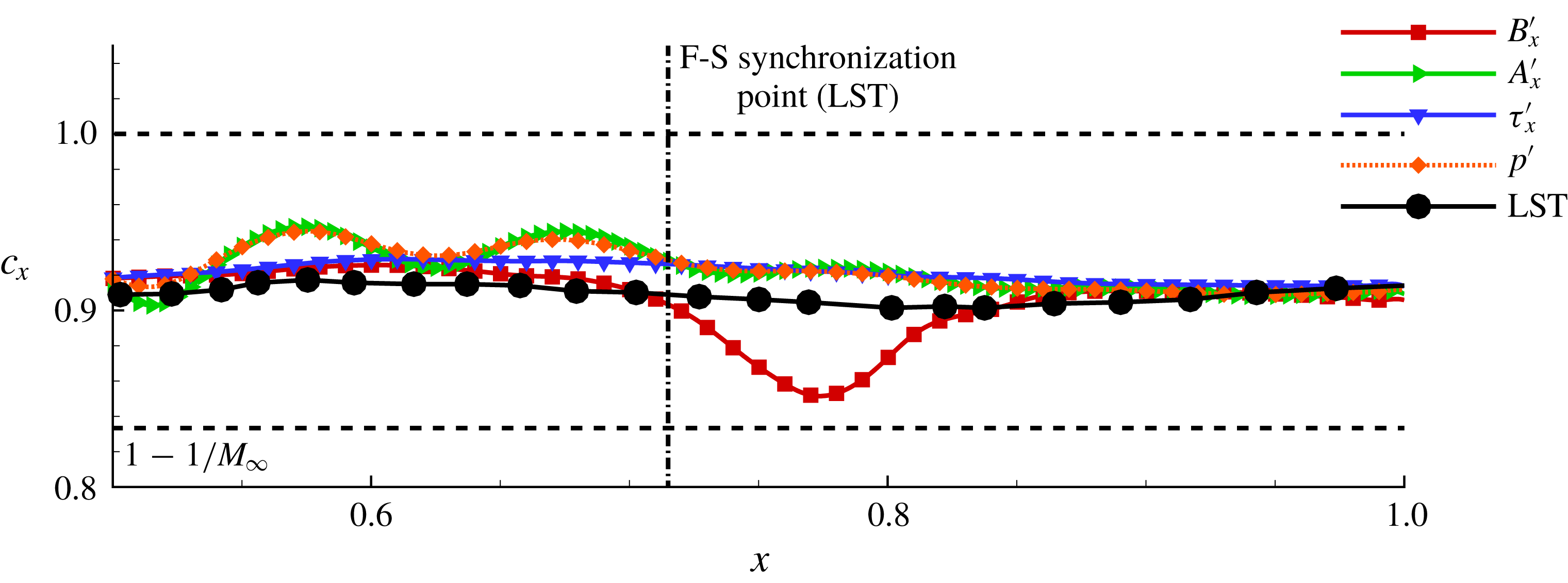
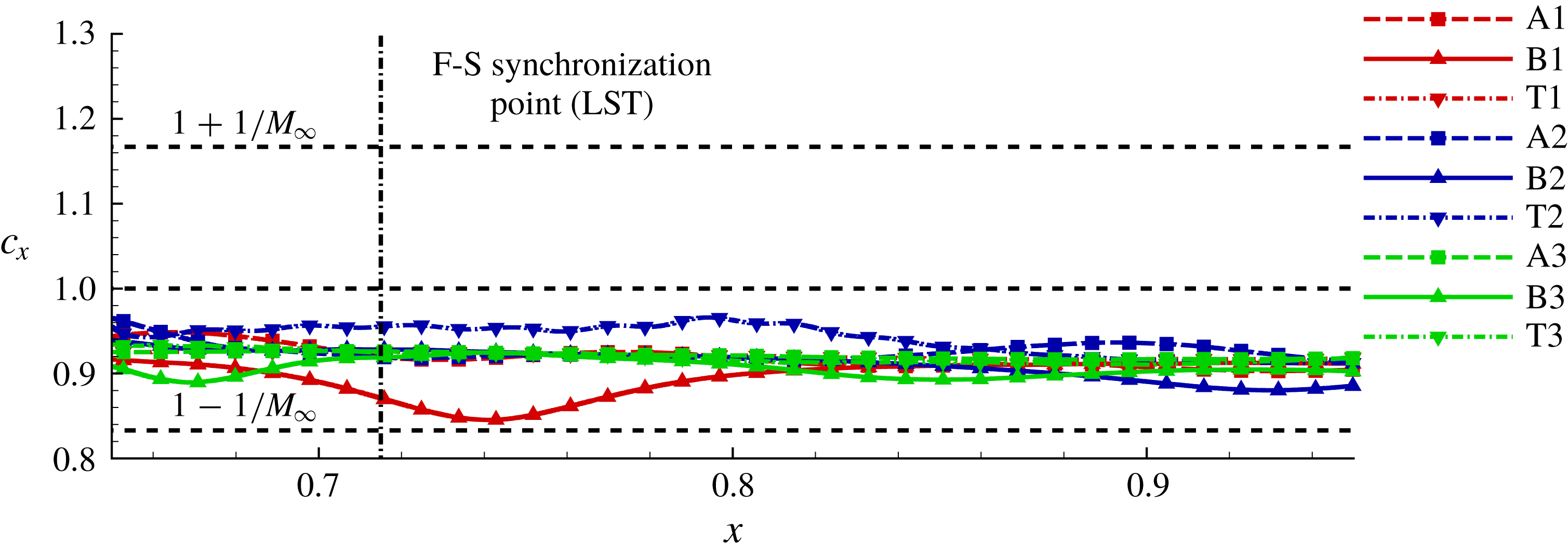
Phase speed variation of instability waves, as obtained from various FT components and pressure, plotted along the streamwise coordinate. The corresponding LST results are also included.

Figure 16 plots the streamwise variation of the phase speeds of pressure fluctuations and the streamwise component of each of the FT components, at a wall-normal distance of
 $y\sim 0.01$
. The phase speeds are obtained from the current DNS calculation using the technique described in Egorov et al. (Reference Egorov, Fedorov and Soudakov2008), which also provides the LST prediction for the slow acoustic component at this forcing frequency,
 $\unicode[STIX]{x1D714}=260$
. For a chosen wall-normal location,
 $y_{0}$
, the phase speeds in a given signal,
 $f_{1}$
(which may be fluctuations in primitive variables or the decomposed FT components), are calculated by first obtaining its zeros, and then using the relation
 $c_{x}\sim \unicode[STIX]{x1D714}\unicode[STIX]{x0394}x/\unicode[STIX]{x03C0}$
, where
 $\unicode[STIX]{x0394}x$
is the spacing between the zeros of
 $f_{1}$
. The forcing results in perturbations with phase speed close to
 $(1-1/M_{\infty })$
, which induces mode S, resulting in the region of second-mode instability. The phase speed variations of pressure fluctuations, acoustic and thermal components are very close to the LST prediction.
An interesting feature is the deviation of the vortical phase speed from linear theory near the FS synchronization point, which is marked by the vertical dotted line. This speed exhibits a local minimum, where the vortical phase speed is less than those of the other components and, in fact, is closer to
 $(1-1/M_{\infty })$
. This behaviour is also consistently observed at other wall-normal locations in the boundary layer, whenever
 $B_{x}^{\prime }$
starts exhibiting second-mode-related amplification. The local minimum in the phase speed of the vortical component is thus inferred to be a consequence of the FS synchronization process, which is identified as the initiation of Mack-mode instability (Ma & Zhong Reference Ma and Zhong2003a
). This indicates a corresponding reduction in the wavelength of the amplifying instability. This localized variation near the FS synchronization point was also confirmed for other frequencies of excitation through multiple DNS results. Thus, phase speed variations in vortical perturbations are also symptoms of FS synchronization, and potential precursors of transition, thus aiding earlier identification of second-mode instability growth. The absence of this trend in the LST based analysis is probably due to the underlying non-parallel effects involved. However, as noted in the discussion surrounding figure 8, the LST results showed a gain in the thermal component of mode S eigenfunction prior to FS synchronization.
5.6 Nonlinear saturation
We now examine the effects of nonlinear saturation on FT dynamics by using the DNS with higher-amplitude perturbations. For this, the amplitude function
 $A$
in (5.1) is set to
 $3.6\times 10^{-2}$
, which is sufficient to engender nonlinear saturation effects. As before, the FT decomposition is applied to the evolving fluctuation field once a fully harmonic solution develops in the entire computational domain.
Perturbation structure within the Mack-mode amplification region with nonlinear saturation. The FT composition of the instability is represented through the contours of the (a,b) vortical, (c,d) acoustic and (e,f) thermal components. The left and right columns show the corresponding streamwise and wall-normal components, respectively. The sonic line and the critical layer are marked using a dash-dotted and a dashed line, respectively.

Figure 17 shows the structure of the decomposed perturbation fields, with contours of the streamwise (left) and wall-normal (right) vortical (first row), acoustic (second row) and thermal (third row) components, respectively. An assessment of the effects of nonlinear development may be made by analysing the differences between corresponding quantities of figures 13 and 17. These effects are most pronounced in the streamwise components of the FT modes. The ‘rope-shaped’ structures in the vortical component (figure 17 a) near the GIP show increased interlacing, consistent with the observations in density fluctuations provided in Egorov et al. (Reference Egorov, Fedorov and Soudakov2006). Below the GIP, the linear and nonlinear vortical features are similar. The tilted recirculation cells appearing around the GIP, observed earlier for linear perturbations, persist in the nonlinear saturation phase. At the current higher perturbation levels, the effect of nonlinearity is primarily to strengthen the vorticity in these cells. Focusing on the near-wall region of recirculation cells that contain negative vorticity, it is clear that this strengthening is accompanied by significant momentum fluctuations opposing the mean flow direction. These higher forcing amplitudes induce local zones of separation on the plate surface.
The primary differences due to nonlinearities in the acoustic component are observed near the wall surface, as evident from figure 17(c,d). Compared to the linear response (figure 13 c,d), the ‘feet’ of the nonlinear acoustic cells lag behind the corresponding structures outside the sonic line. These regions eventually detach from the larger lobes, resulting in smaller structures over the wall, corresponding to higher harmonics in the perturbation field. The nonlinear thermal response (figure 17 e,f) again reveals features that are generally similar to the vortical component, in that the effects are limited to the region near the GIP, where increased distortion of the perturbation lobes is observed.
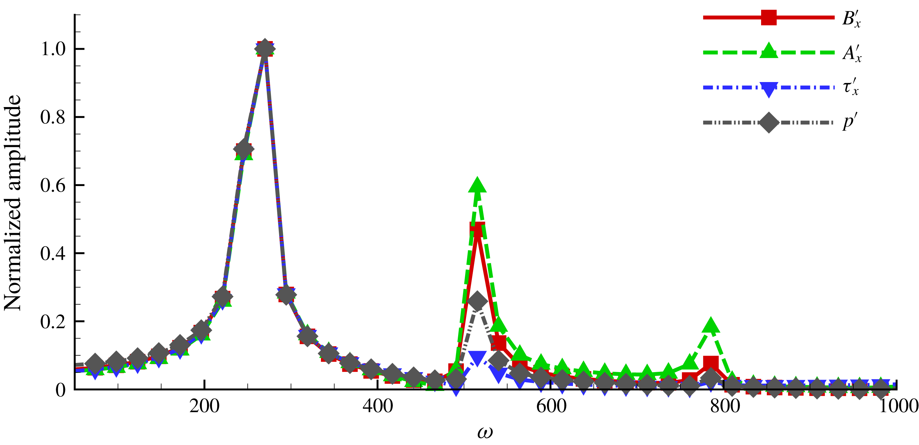
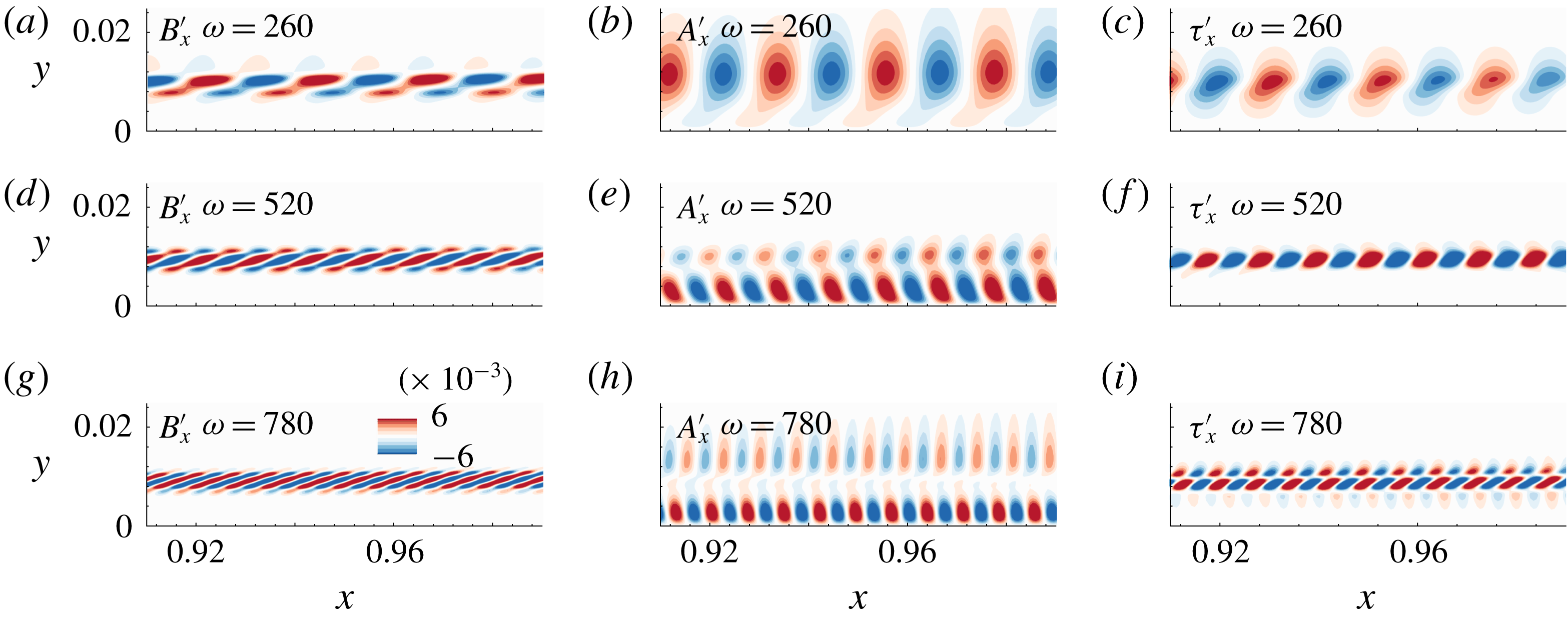
The modified modal shapes in the nonlinear response are a manifestation of superharmonics in the HBL. Spectral analyses of probe data at various locations in the boundary layer indicate the presence of two superharmonics in pressure perturbations, corresponding to
 $\unicode[STIX]{x1D714}=520$
and
 $\unicode[STIX]{x1D714}=780$
(Egorov et al.
Reference Egorov, Fedorov and Soudakov2006). For example, figure 18 shows the normalized amplitude (with respect to the fundamental) of the power spectrum of the vortical, acoustic, thermal and pressure perturbation signals at a point just over the plate surface, at
 $x\sim 0.9$
, which lies in the amplified second-mode region. The fundamental and the two superharmonics are clearly visible. An interesting aspect here is the relative prominence of the superharmonics compared to the fundamental. The heights of the peaks at
 $\unicode[STIX]{x1D714}=520$
and 780 indicate that, at this location, nonlinearities are most pronounced in the acoustic component. Thus the nonlinear saturation occurs at different rates, with specific FT components being responsible for introducing saturated frequencies at different locations in the boundary layer.
Normalized power spectrum of the FT components and pressure fluctuations in the nonlinearly saturated case. Spectra shown at the near-wall location at
 $x\sim 0.9$
.

In order to assess this spatial effect, we identify zones in the HBL that are susceptible to nonlinear saturation, and the physical components responsible for inducing such effects. This requires the extraction of frequency-isolated dynamically growing components in the flow. Several popular techniques have been proposed or modified to extract such modes (not directly related to stability modes) – a recent survey may be found in Taira et al. (Reference Taira, Brunton, Dawson, Rowley, Colonius, McKeon, Schmidt, Gordeyev, Theofilis and Ukeiley2017) and a connection between some methods has been outlined in Towne, Schmidt & Colonius (Reference Towne, Schmidt and Colonius2018). In the present work, we consider dynamic mode decomposition (DMD) (Schmid Reference Schmid2010), which is better for this purpose than the more common proper orthogonal decomposition (POD) technique, because it extracts the spectral content of a snapshot series, together with the corresponding spatial support. DMD modes thus provide the spatial distribution of the fundamental and superharmonic content in the response.
DMD modes of the vortical (a,d,g), acoustic (b,e,g) and thermal (c,f,i) components. Each row corresponds to a specific frequency, as denoted.

The results of DMD analysis are shown in figure 19. The three columns of figure 19 show DMD modes of the vortical, acoustic and thermal components, respectively, at three frequencies (rows), specifically
 $\unicode[STIX]{x1D714}=260$
, 520 and 780, which are the fundamental and the first two superharmonics, respectively. The phase speeds of all the DMD modes are plotted in figure 20 at a representative height of
 $y\sim 0.01$
. These are denoted as A1 (acoustic), B1 (vortical) and T1 (thermal). The corresponding values for the first and second superharmonics are A2, B2, T2 and A3, B3, T3, respectively. The local minimum in the vortical phase speed (discussed earlier in the context of figure 16) is only observed at the fundamental frequency. Similar phase speeds at various frequencies indicate a proportionate reduction in the wavelength of these pure frequency modes. DMD modes also possess growth rates, which are not discussed because they are inconsequentially small for the statistically stationary state examined.
Phase speeds of DMD modes of the acoustic, vortical and thermal components. The phase speeds of the fundamental DMD mode of the acoustic, vortical and thermal components are represented as A1, B1 and T1, respectively; A2, B2, T2 and A3, B3, T3 are the phase speeds of the first and second superharmonics of the FT components, respectively.

The spatial supports of all frequencies of the vortical component (figure 19 a,d,g) are primarily restricted to the vicinity of the GIP. The superharmonics (figure 19 d,g) have a finer rope-shaped nature, which results in the heightened interlacing and distortion of the nonlinear vortical response discussed in figure 17. Acoustic perturbations in the nonlinear regime (figure 19 b,e,h), show a more extensive spatial distribution. The fundamental mode has peak values just above the critical layer (as expected from the linear scenario), whereas the superharmonics are dominant closer to the plate surface. One consequence is the existence of fine-scale acoustic waves near the wall, bounded by the sonic line. Thus, the acoustic component introduces nonlinear saturation nearer to the wall. The nonlinear development of the flow near the wall may therefore be more susceptible to acoustic perturbations from suitable actuators. The thermal response in figure 19(c,f,i) indicates that the fundamental mode is most prevalent in the boundary layer. The superharmonics are limited around the GIP and have minimal presence in the region closer to the plate surface. This demarcation using DMD of FT harmonics in the boundary layer has the potential to yield reduced-order models or low-rank representations of second-mode instabilities in HBLs.
These nonlinear saturation effects on the second mode were tested for various Mach numbers ranging from 6 to 8 with adiabatic and cold walls (wall cooled to 70 % of the corresponding adiabatic wall temperature), as well as blowing–suction and free-stream methods of imposing perturbations. In all cases, the results were observed to be similar to those discussed above.
5.7 Effect of wall cooling
The sensitivity of transition to the wall thermal condition has been described in numerous efforts. The second mode of current focus is destabilized by wall cooling, as observed experimentally (Stetson et al. Reference Stetson, Thompson, Donaldson and Siler1989; Stetson & Kimmel Reference Stetson and Kimmel1992) and confirmed through theoretical and numerical observations (Mack Reference Mack1975). To understand this sensitivity, we now analyse FS synchronization over a cooled plate, by repeating the above analyses with a cold wall, whose temperature is reduced to 70 % of the corresponding adiabatic wall value. Results with LST are discussed first, followed by those of the DNS.
Effect of wall cooling on LST amplification rate,
 $\unicode[STIX]{x1D714}_{i}$
. The adiabatic and cold wall rates are shown as a function of perturbation wavelength,
 $\unicode[STIX]{x1D706}$
.

Figure 21 plots the temporal growth rate,
 $\unicode[STIX]{x1D714}_{i}$
, versus streamwise wavelength,
 $\unicode[STIX]{x1D706}$
, for both the adiabatic and cooled wall conditions, at a representative location
 $x=1.2$
. As expected, cooling amplifies the growth rate of mode S, resulting in an increase in the peak value of
 $\unicode[STIX]{x1D714}_{i}$
. The region of instability (
 $\unicode[STIX]{x1D714}_{i}>0$
) shifts to the left, indicating the susceptibility of smaller-wavelength waves to amplify, consistent with prior observations (Lysenko & Maslov Reference Lysenko and Maslov1984; Zhang, Liu & Luo Reference Zhang, Liu and Luo2016). Cooling shifts the outer GIP (already present in the adiabatic case) closer to the plate surface and also results in the formation of an inner GIP, in close proximity to the wall (Masad, Nayfeh & Al-Maaitah Reference Masad, Nayfeh and Al-Maaitah1992). The second mode is consistently found to exhibit peak perturbation values in the vicinity of the outer GIP. Under cold wall conditions, this generally leads to smaller length scales between the GIP/critical layer and the wall, and dictates the internal reflection scale of the acoustic component, as was observed in figure 6(b,e).
Cold wall results. (a) Variation of phase speeds of mode S and mode F across the FS synchronization point. Variation of the (b) vortical, (c) acoustic and (d) thermal content in mode S during FS synchronization.

Continuing with the LST-based analysis, the influence of cooling on FS synchronization and the associated FT behaviour is shown in figure 22. As in the analysis for the adiabatic case (figure 8), we consider the evolution of mode S and mode F with
 $\unicode[STIX]{x1D706}=0.025$
. Their phase speed variation is plotted in figure 22(a), and the vortical, acoustic and thermal components of mode S are presented in figure 22(b), 22(c) and 22(d), respectively. Upon cooling the wall, the fluctuation at a given wavelength undergoes synchronization further downstream, in this case at
 $x\sim 0.93$
(compared to
 $x\sim 0.7$
for the adiabatic wall). The vortical component continues to be the dominant one in terms of displaying the highest amplitude among all the FT components. The peaks of all three components now appear closer to the wall due to the downward shift of GIP in the cooled boundary layer. As observed in figure 22(c) and 22(d), respectively, the precursor thermal component amplification activity identified earlier, as well as the acoustic component amplification near the vicinity of the FS synchronization point, are also consistently reproduced in the cold wall analysis.
The above LST results are now augmented with an analysis of cold wall DNS calculations, using the same wall temperature conditions. Various techniques of forcing were utilized, including wall blowing–suction and free-stream acoustic disturbances. Since the observations are qualitatively similar, and independent of forcing type, we focus for brevity on those obtained with free-stream acoustic wave forcing. Since second-mode instabilities in the HBL are more receptive to free-stream slow acoustic waves (Ma & Zhong Reference Ma and Zhong2005), the forcing utilizes a monochromatic free-stream wave with a phase speed
 $(1-1/M_{\infty })$
. The free-stream pressure fluctuations, following Egorov et al. (Reference Egorov, Fedorov and Soudakov2008), have an amplitude of
 $|p^{\prime }|=5\times 10^{-5}$
, and the velocity fluctuations of this wave at zero angle of incidence on the plate are specified as
 $u^{\prime }=-M_{\infty }|p^{\prime }|$
and
 $v^{\prime }=0$
. The amplitude of free-stream temperature fluctuations is
 $|T^{\prime }|=(\unicode[STIX]{x1D6FE}-1)M_{\infty }^{2}|p^{\prime }|$
. The waves have a pure harmonic form, and an FT decomposition shows that all fluctuations upstream of the leading-edge shock wave are fully represented in the acoustic component, as the forcing perturbations do not contain vorticity, and the mean flow is devoid of any gradients. Several forcing frequencies were simulated: the results presented here are obtained for a forcing frequency of
 $\unicode[STIX]{x1D714}=240$
, which ensures that the peak amplification of the Mack mode occurs in the well-resolved part of the computational domain for both adiabatic and cold wall cases. This also maintains the perturbation wavelengths close to the values observed in the previous sections. Furthermore, the forcing amplitude,
 $5\times 10^{-5}$
, is small enough to preserve linearity in the perturbation field.
Magnitude of the (a) vortical, (b) acoustic and (c) thermal components under identical forcing conditions over an adiabatic and a cold plate.

The effects of wall cooling are first analysed by examining the streamwise variation of perturbation amplitudes of the individual FT components. Figures 23(a), 23(b) and 23(c), respectively, show the magnitudes of the vortical, acoustic and thermal components at a wall-normal location of
 $y\sim 0.01$
. In each panel, the corresponding adiabatic (ADB) and cold (COLD) wall results are plotted using solid and dotted lines, respectively. The peak value in each plot corresponds to the second-mode instability in the corresponding boundary layer. As predicted by the linear analysis (§ 4), the region of second-mode amplification begins at
 $x\sim 0.7$
and
 $x\sim 0.9$
for the adiabatic and cold walls, respectively. The peak vortical fluctuations are significantly lower over the cooled wall than those observed for the adiabatic wall. This is generally consistent with prior observations of lower peak amplitude in cooled walls compared to adiabatic walls, attributable to the receded streamwise location of the neutral curve and the associated smaller values of perturbations (see e.g. Liang et al.
Reference Liang, Li, Fu and Ma2010). Despite this, the acoustic component exhibits a higher rate of amplification, as well as attains a slightly higher peak value in the cold wall simulation. Upon cooling, the thermal component also shows attenuation, like the vortical perturbations. Thus, although the largest perturbations in the Mack mode are vortical, the destabilization associated with wall cooling is a consequence of the dynamics of the acoustic component.
6 Energy considerations
As mentioned in § 1, MPT provides conservation laws that govern the evolution of instabilities in the context of their FT content, and the manner in which these perturbations interact with each other. The FT decomposition of the instability eigenfunctions in § 4.2 highlighted the activation of acoustic perturbation growth during FS synchronization and prior amplification of the thermal component. Such dynamics was also observed in the corresponding DNS analyses. Clearly, the change in energy associated with each FT component is a consequence of interactions between different disturbance components and the mean flow. An elegant approach to quantify these changes is through the TFE budget, discussed in § 2. Specifically, variations in the TFE due to each component can be correlated with the corresponding source terms in the energy balance, as represented by the TFE equation (2.7). We now analyse the DNS data in this manner for both adiabatic and cold walls by evaluating each term in the TFE equation of § 2. The term ‘sources’ as used here also refers to sinks, depending on sign, and act as production or dissipation terms of enthalpy. Thus, positive sources contribute to the production of TFE, while negative sources are effectively sinks, and dissipate TFE.
TFE source mechanisms. (a–f) Various TFE source terms as indicated: (a,c,e) the vortical, acoustic and thermal TFE sources for the adiabatic wall; (b,d,f) the vortical, acoustic and thermal TFE sources for the cold wall. The contours are plotted in the vicinity of Mack-mode amplification. The stretched wall-normal coordinate is
 $y5=5\times y$
, and is used to highlight the region with dominant source activity. (g) Axial distribution of TFE sources at
 $y=0.002$
for the adiabatic wall. (h) Axial distribution of TFE sources at
 $y=0.002$
for the cold wall.

Figure 24 examines the FT-component-induced sources responsible for enthalpy fluctuations, by analysing the three major terms in the TFE equation, i.e.
 $-(\boldsymbol{B}^{\prime }\boldsymbol{\cdot }\unicode[STIX]{x1D736}^{\prime })$
,
 $-(\boldsymbol{A}^{\prime }\boldsymbol{\cdot }\unicode[STIX]{x1D736}^{\prime })$
and
 $-(\unicode[STIX]{x1D749}^{\prime }\boldsymbol{\cdot }\unicode[STIX]{x1D736}^{\prime })$
. We designate these as vortical, acoustic and thermal, respectively, based on the presence of the three components in those source terms. Figure 24(a,c,e) display the spatial distribution of the vortical, acoustic and thermal sources, respectively, for the adiabatic wall. Figure 24(b,d,f) are the corresponding sources for the cooled wall. Figure 24(g,h) plot the streamwise variation of the three source terms at a representative wall-normal height of
 $y=0.002$
, in close vicinity of the plate surface. In order to provide a relative perspective, all the source terms are normalized by the peak value of the vortical source,
 $-(\boldsymbol{B}^{\prime }\boldsymbol{\cdot }\unicode[STIX]{x1D736}^{\prime })$
, of the adiabatic plate.
The observations are characterized by distinguishing effects prior to FS synchronization from those thereafter. The primary source of TFE within the boundary layer prior to the FS synchronization location is vortical in nature: it is always localized in the vicinity of the GIP, and is relatively weaker closer to the plate surface. Although not included in the axial range shown here, prior to the FS synchronization point, the vortical term also induces a weak source region between the GIP and the plate surface. However, this term switches sign to become a prominent sink (dissipating TFE) in the second-mode amplification region, as can be clearly seen in figure 24(a), in the range
 $1<x<1.2$
. This implies that the vortical component dissipates TFE in the region of maximum Mack-mode amplification (figure 24
a,b).
The acoustic production is the weakest of all sources, and has a minor contribution within the boundary layer (figure 24 c,d). While the thermal source term remains insignificant prior to synchronization, it dominates TFE production during the destabilization of the second mode. Indeed, this positive source term sustains the generation of TFE in the Mack mode, particularly within the ‘trapped’ region.
These source/sink behaviours and trends are consistent between the adiabatic and cooled walls, though there are quantitative differences. A key observation is that, although the vortical component is stabilized (smaller fluctuation amplitudes) through wall cooling, the peak value of the vortical dissipation term actually increases. This is evident from a comparison of peak negative contour values of figure 24(a,b), and the most negative value attained by the (red) dash-dotted lines in figure 24(g,h). However, the thermal sources are less sensitive to wall cooling, and thus become more important in generating TFE sources and destabilizing the boundary layer under cooled wall conditions. Figure 24(g,h) confirm these general observations by considering the individual source and sink terms at a fixed distance (
 $y=0.002$
) away from the wall for the adiabatic and cold wall cases, respectively. The switching of the vortical term, (red) dash-dotted lines, from a very weak source (positive values) to a strong sink (negative values) inside the boundary layer is also evident, together with the simultaneous development of the thermal source, (blue) dashed lines, displaying positive values. For example, in the adiabatic case, figure 24(g), the vortical source term is slightly positive at
 $x<0.7$
, whereas it changes its sign to become predominantly negative in the range
 $0.8<x<1.2$
. Consistent trends can also be seen in the source terms of the cold wall case, figure 24(h).
Components of thermal source in the region of second-mode amplification. Source terms due to thermal interactions with fluctuating (a) Lamb vector and (b) entropy gradients. The contours are plotted in the vicinity of Mack-mode amplification. The stretched wall-normal coordinate is
 $y5=5\times y$
, and is used to highlight the region with dominant source activity.

Since the thermal component was identified as a major contributor to fluctuating energy in the boundary layer instability zone, details of the responsible source mechanisms for the cold wall are presented in figure 25, whose spatial range is consistent with that shown in figure 24. Figure 25(a) shows the distribution of the first component of thermal sources due to the interaction with Lamb vector fluctuations,
 $-({\unicode[STIX]{x1D749}^{\prime }\boldsymbol{\cdot }\unicode[STIX]{x1D736}}_{1}^{\prime })$
. Figure 25(b) shows the result of thermal–entropic interactions,
 $-({\unicode[STIX]{x1D749}^{\prime }\boldsymbol{\cdot }\unicode[STIX]{x1D736}}_{2}^{\prime })$
. The first component is relatively weaker in magnitude, but displays peaks within the lower region, closer to the plate surface. The thermal–entropic source has a much higher magnitude, and is prominently located around the GIP, due to the heightened vorticity-induced entropic fluctuations generated there.
7 Conclusions
The evolution of vortical, acoustic and thermal content (designated as fluid-thermodynamic (FT) components), and their interactions with each other, are described to augment the linear and nonlinear growth of stability modes in a hypersonic boundary layer. To this end, momentum potential theory is applied to results from linear stability theory and direct numerical simulations, the latter using wall blowing–suction as well as free-stream disturbances. Particular emphasis is placed on the effects encountered in the vicinity of the FS (fast–slow) synchronization point, the subsequent linear and nonlinear saturation dynamics, and the effects of wall cooling. Although vortical disturbances comprise the most prominent perturbation component, with peaks near the generalized inflection point (GIP), thermal and acoustic components are more dynamic, i.e. change most rapidly, in the region of interest. Fluxes associated with vortical components form rope-like structures straddling the GIP, and carry momentum fluctuations across it: their overall form is similar to structures observed in flow visualizations. However, the acoustic and thermal perturbation fluxes exhibit trapped structures: the former between the wall and the critical layer in the manner of a waveguide, the latter between the wall and a wavy locus straddling the GIP. The upper boundary of each trapped domain comprises a series of alternating monopoles. The results show that the phase speed of the vortical component displays a local minimum in the vicinity of the synchronization point, the thermal component is excited prior to it, while the acoustic component grows rapidly after it.
The effects of nonlinear saturation manifest in the generation of two superharmonics, whose features are substantially different from each other for the three FT components. The fundamental response of the vortical component retains its rope-like structure but, under nonlinear growth, distorts and aligns more closely with the flow direction, with generation of superharmonics near the GIP. The fundamental response of the acoustic component shows peaks just above the critical layer, but the superharmonics occur closer to the wall surface, indicating the sensitivity of the region between the wall and the sonic line following linear growth. Cooling the boundary layer results in damping of both vortical and thermal perturbations. However, acoustic perturbations increase slightly: the relative acoustic component is thus larger with wall cooling.
The dynamic interaction between the different components, examined through the effects on total fluctuating enthalpy (TFE), suggest that, in the region of maximum growth, the nature of vortical sources of TFE switch from a production term to a dissipation term. The term containing the thermal component, on the other hand, becomes the primary source of TFE. The analysis in this paper thus provides a clearer association between stability modes and their FT characteristics, without solely relying on their phase speeds for such classifications. This facilitates new insight into the nature and sources of perturbation growth in high-speed transition.
Future work will examine the manner in which proposed control techniques interfere in growth of instabilities, with the objective of optimizing inputs that target individual FT components. The procedure also facilitates an examination of resonant mechanisms in the nonlinear regime and three-dimensional breakdown through energy dynamics.
Acknowledgements
This research was supported by the Office of Naval Research (grants N0001-13-1-0534, N00014-17-1-2584) monitored by E. Marineau, with R. Burnes serving as technical point of contact. We are grateful for extended conversations with Professor A. Tumin and Dr M. Choudhari. The simulations were performed with a grant of computer time from the DoD HPCMP DSRCs at AFRL, NAVO and ERDC, and the Ohio Supercomputer Center.