1. Introduction
Legged robots show strong potential in planetary exploration, disaster response, and operations in extreme environments because of their adaptability to unstructured terrain. However, these robots are prone to high failure rates resulting from component malfunctions, such as joint locking and actuator damage under complex working conditions, which lead to mission interruptions and elevated repair costs, severely constraining their practical deployment efficacy. Fault-tolerant (FT) mechanisms are thus essential for multi-legged robots to maintain mobility after leg failure, enhancing their practicality and reliability. Current FT strategies for legged robots are broadly categorized into the following two paradigms: gait replanning methods and posture regulation or the use of auxiliary devices.
For hexapod robots experiencing the loss of a single leg, gait replanning is the predominant approach, leveraging inherent limb redundancy to reconstruct stable gaits. Yang’s team [Reference Yang and Kim1] pioneered this field by developing a tripod gait planning method based on static stability margins (SSMs), establishing a framework for sustained locomotion. Under their scheme, the hexapod robot employs a modified tripod gait to continue efficient movement after a leg failure. They further proposed a FT gait sequence using crab walking on even terrain [Reference Yang and Kim2], which relaxes the non-overlap constraint in redefined reachable leg workspaces and incorporates crab motion [Reference Yang and Kim3]. Validation of this strategy on uneven terrain contributed to the theoretical framework of fault-tolerance for static walking in legged robots [Reference Yang and Kim4]. To address locked joint failure, a FT tripod gait strategy was proposed [Reference Yang5]. Additionally, a Follow-The-Leader (FTL) gait strategy was developed for post-failure walking, combining fault tolerance with enhanced terrain adaptability [Reference Yang6]. Du et al. [Reference Du and Gao7] presented a motion planning method employing linear FT Jacobian matrices, enabling the execution of desired motions using impaired legs alongside compensatory concomitant movements. More recently, Cui et al. [Reference Cui, Li, Qiu and Li8] proposed a FT motion planning framework for quadruped robots with joint-lock faults by combining posture optimization with whole-body control. Single-leg failures in quadruped robots are commonly mitigated through attitude control or auxiliary devices to ensure fault tolerance. While Pan’s support triangle principle confirms static stability with a single leg missing, its applicability is limited in double-leg failure scenarios due to spatial constraints [Reference Pan, Gao and Du9]. Chen et al. [Reference Chen, Gao, Xi and Zhao10] modeled the foot-tip of a locked leg as a passive rotational joint, proposing a FT gait with non-zero SSMs that facilitates omnidirectional walking and turning on rough terrains. You et al. [Reference You, Fan and Liu11] adopted a foot force control strategy to improve robustness and stability in six-legged robots with single-leg failure, advancing FT motion planning.
Single-leg failures in quadruped robots are commonly mitigated through attitude control or auxiliary devices to ensure fault tolerance. For instance, Paredis [Reference Paredis12] designed a series FT manipulator that significantly enhances motion controllability under joint failure conditions. Lee’s team [Reference Lee and Hirose13] developed a kicking-swinging coordinated three-legged gait for four-legged mine clearance robots, incorporating active vibration reduction to facilitate motion recovery. Gor et al. [Reference Gor, Pathak, Samantaray, Yang and Kwak14] proposed a fault tolerance strategy for actuators/sensors via a device that adjusts the back center of gravity (COG) in a quadruped configuration. Cho et al. [Reference Cho, Min and Kim15] combined gait stability with inertial moment control to increase the stability margin. Additionally, Goerner [Reference Görner and Hirzinger16] enhanced post-failure walking capability through the use of mobile gears and adaptive flexible joints.
Furthermore, computational intelligence techniques such as genetic algorithms and reinforcement learning have been introduced to enhance damage tolerance in legged robots [Reference Faigl and Čížek17]. For instance, Luo et al. developed a FT control pipeline named FT-Net, which utilizes model-free reinforcement learning to enable seamless transition from quadruped to tripodal locomotion in the event of complete motor failure [Reference Luo, Xiao and Lu18]. Similarly, Hou et al., employed a multi-task training architecture designed to actively perceive and compensate for two distinct types of leg-joint faults [Reference Hou, Tu, Gao, Dong, Zhai and Zhang19]. Nevertheless, these methods remain largely focused on gait reconfiguration in hexapod robots and are constrained by several limitations, including high computational cost, low sample efficiency, and training instability. These issues often lead to slow adaptation, suboptimal policy generation, and limited generalization to unseen damage conditions or changing environments. Recent learning-based studies have extended FT locomotion in quadrupeds to more complex fault scenarios, such as multiple joint faults and motor-stuck conditions [Reference Chen, Li, Lu, Wang and Xiong20, Reference Xu, Cheng, Shen and Zhao21]. However, these methods are still mainly developed for quadruped platforms and generally rely on substantial training.
Although existing studies have shown that effective fault tolerance for localized damage, such as single-leg failure, can be achieved by adjusting the median angle of the body-coxa joint during the stance phase to maintain the COG within a stable support polygon [Reference Zhang, Zhang, Ma, Li and Fang22]; however, more severe damage, such as ipsilateral two-leg failure, remains unsolved and presents considerable challenges in stability control. Inspiration can be drawn from biological locomotion mechanisms. Certain insects equipped with specialized appendages, such as the raptorial forelegs of mantises, saltatory hindlegs in grasshoppers, or fossorial forelegs in mole crickets, can employ “functional-leg substitution” to regain mobility when their walking legs are impaired [Reference Zhang, Zhang and Ren23]. Similarly, equipping legged robots with a functional arm (FA) has become a common approach to support complex tasks, including pipe connection, assembly, and grasping [Reference Tefera, Bianchi, Carbonaro, Tognetti and Dosen24]. For example, Zhao et al. proposed a multimodal quadruped robot capable of reusing a single limb for both walking and manipulation [Reference Zhao, Wu, Yang, Ding, Xu, Guo and Jin25]. Deploying the FA as a substitute for a lost walking leg not only expands its functional utility but also improves overall availability without introducing additional mechanical redundancy.
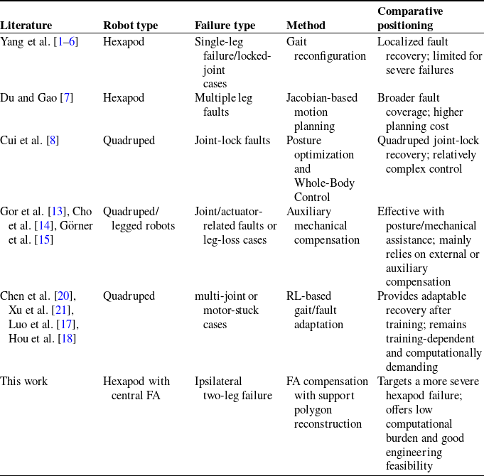
While research on utilizing multifunctional limbs for task assistance and gait reconfiguration for single-leg failure has progressed, existing methods still exhibit clear limitations when addressing the extreme failure of ipsilateral two-leg failure, which causes severe destabilization of the robot. Traditional gait reconfiguration heavily relies on the redundancy of the remaining legs to maintain the support polygon, whereas existing studies on multifunctional limbs primarily focus on the extension of operational capabilities and have not systematically explored their potential for locomotion recovery under severe walking impairments. To bridge this research gap, this paper innovatively proposes redefining the FA, originally designed for manipulation tasks and mounted at the center of the hexapod body, as an active walking leg. By reconstructing the robot’s support polygon through optimal foothold planning. Compared to previous studies, as summarized in Table I, this work addresses a more severe failure scenario – ipsilateral two-leg failure in a hexapod robot – thereby providing a new FT solution for multi-legged robots with low computational demand and good engineering feasibility.
Comparison of representative fault-tolerance studies and the proposed method.

Table I Long description
A table comparing fault-tolerance studies and methods for different robot types and failure scenarios. The table has six columns: Literature, Robot type, Failure type, Method, and Comparative positioning. It contains nine rows, including a header row. Row 1: Literature, Robot type, Failure type, Method, Comparative positioning. Row 2: Yang et al., Hexapod, Single-leg failure/locked-joint cases, Gait reconfiguration, Localized fault recovery; limited for severe failures. Row 3: Du and Gao, Hexapod, Multiple leg faults, Jacobian-based motion planning, Broader fault coverage; higher planning cost. Row 4: Cui et al., Quadruped, Joint-lock faults, Posture optimization and Whole-Body Control, Quadruped joint-lock recovery; relatively complex control. Row 5: Gor et al., Cho et al., Grner et al., Quadruped/legged robots, Joint/actuator-related faults or leg-loss cases, Auxiliary mechanical compensation, Effective with posture/mechanical assistance; mainly relies on external or auxiliary compensation. Row 6: Chen et al., Xu et al., Luo et al., Hou et al., Quadruped, multi-joint or motor-stuck cases, RL-based gait/fault adaptation, Provides adaptable recovery after training; remains training-dependent and computationally demanding. Row 7: This work, Hexapod with central FA, Ipsilateral two-leg failure, FA compensation with support polygon reconstruction, Targets a more severe hexapod failure; offers low computational burden and good engineering feasibility.
The remainder of this paper is organized as follows. Section 2 details the mechanical architecture of the FA-integrated hexapod platform. Section 3 analyses two-leg failure scenarios and introduces an FA positioning strategy optimized based on longitudinal stability margin criteria. Section 4 provides theoretical verification of the compensation mechanism. Finally, Section 5 demonstrates the effectiveness of locomotion recovery through prototype experiments with FA compensation.
2. Structure of the functional arm hexapod robot
The FA hexapod robot comprises of the following three main components: the main robot body, six locomotor legs, and an FA centrally mounted on the body, as shown in Figure 1(a). The FA is attached to the body via a rotary base with five degrees of freedom (DOF). Although the FA end-effector can be equipped with operational tools such as grippers, this study utilizes a non-slip rubber pad for enhanced ground contact. The six legs are symmetrically arranged along the major and minor axes of the body and are denoted as LF, LM, LH, RF, RM, and RH, as indicated in Figure 1(b), where L and R refer to the left and right sides, respectively, and F, M, and H denote the front, middle, and hind legs, respectively. The origin of the robot’s three-dimensional coordinate system is set at the COG, defined as O 0, with the y-axis aligned in the direction of motion and the x-y plane parallel to the ground. To prevent interference between adjacent legs, the angular range of motion for each leg is set to ±36°. Accounting for practical operational conditions and ensuring a safety margin, the angular range of each leg is limited to ±20°.
Schematic diagram of the FA hexapod robot mechanism. (a) The 3D model of the FA hexapod robot. (b) The FA hexapod robot leg layout. (c) The structure of a single leg. (d) The structure of functional arm (FA).

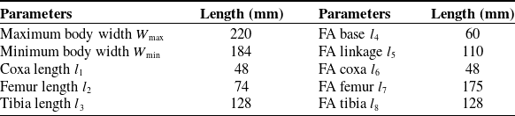
Figure 1(c) shows the structure of a single leg, comprising the following three main segments: the coxa, femur, and tibia. The local coordinate system of each leg is defined at its origin Oi , with θi representing the joint angle. The lengths of the coxa, femur, and tibia are designated as l 1, l 2, and l 3, respectively. As shown in Figure 1(d), the FA incorporates a five-DOF linkage mechanism, composed of a base, linkage, coxa, femur, tibia, and five joints. The corresponding lengths are denoted as l 4, l 5, l 6, l 7, and l 8, respectively, with detailed dimensional parameters provided in Table II.
Dimensional parameters of the FA hexapod robot.

Table II Long description
A table comparing dimensional parameters of a hexapod robot. The table has two columns and ten rows. The first column lists parameters related to the body and leg segments of the robot, and the second column provides the corresponding lengths in millimeters. Row 1: Maximum body width W max, 220. Row 2: Minimum body width W min, 184. Row 3: Coxa length l 1, 48. Row 4: Femur length l 2, 74. Row 5: Tibia length l 3, 128. Row 6: FA base l 4, 60. Row 7: FA linkage l 5, 110. Row 8: FA coxa l 6, 48. Row 9: FA femur l 7, 175. Row 10: FA tibia l 8, 128.
3. FA compensation strategy for ipsilateral two-leg failure
3.1. Failure scenario analysis
The robot’s body is symmetric about the y-axis, with the FA mounted at its geometric center. As a result, ipsilateral two-leg failure presents two distinct configurations, middle-front/hind leg failure (Figure 2(a), (b)), and front-hind leg failure (Figure 2(c), (d)). During a gait cycle, the robot exhibits both stable (Figure 2(a), (c)) and unstable (Figure 2(b), (d)) states under each of these failure scenarios.
Instability conditions under ipsilateral two-leg failure. (a) and (b) show RM and RH (RM + RH) failure, (c) and (d) show RF and RH (RF + RH) failure.

Taking the RM + RH failure as an example, when Leg 1 (LF) is in the swing phase, the remaining legs form a support triangle B-C-D that contains the projection of COG, thereby maintaining robot stability (Figure 2(a)). In contrast, when Leg 4 (RF) enters the swing phase, the displacement of the COG outside the support triangle A–B–C leads to instability (Figure 2(b)). Because the legs are arranged symmetrically along the body axis in typical hexapod robots, they cannot rotate circumferentially around the body [Reference Chen, Zhong, Liu and Deng26, Reference Zhong, Chen and Deng27]. Therefore, the instability in Figure 2(b) and (d) cannot be resolved using posture-regulation strategies, such as adjusting foot positions [Reference Liu, Fan, Ding, Wang, Liu and Gao28] or body inclination. To address this, the present study introduces a FA compensation mechanism for conventional hexapods, optimizing the compensatory placement to replace failed legs and achieve FT recovery under destabilizing failure conditions.
3.2. Gait selection and foot-end position definition
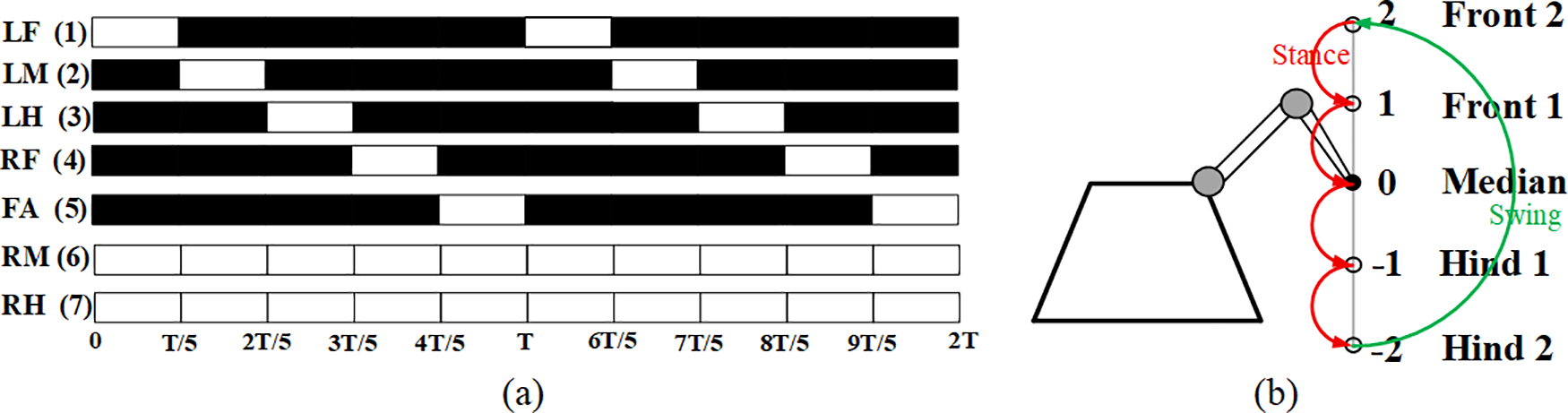
When compensating for ipsilateral two-leg failure using the FA, the wave gait is employed to maintain fundamental mobility [Reference Yang29]. Under this scheme, five legs participate in locomotion, ensuring that four legs remain in the stance phase at any given instant. Taking the RM + RH failure as an example, the swing sequence initiates at T = 0 in the order LF→LM→LH→RF→FA. As indicated in Figure 3(a), within the gait sequence diagram, black blocks represent stance phases, whereas white blocks correspond to swing phases.
Gait sequence and foot-end position diagram. (a) RM + RH failure, FA compensation wave gait sequence diagram. (b) Foot-end relative body position diagram.

During the wave gait cycle, the motion trajectory of a single leg is characterized by five distinct positions, as depicted in Figure 3(b). Taking the RF leg as an example, these positions correspond to specific time points in the cycle: at time 4T/5, the foot-end reaches the foremost extreme position (designated as front 2 and labeled as number 2); at time T, it is at the front 1 position (number 1); at time T/5, it passes through the middle position (middle 0, number 0); at time 2T/5, it moves to the hind 1 position (number −1); and at time 3T/5, it arrives at the rearmost extreme position (hind 2, number −2).
3.3. FA compensation position optimization
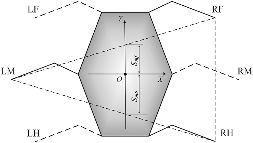
This study investigates the scenario in which a hexapod robot experiences drastic support polygon deformation due to ipsilateral two-leg failure during straight-line walking. The longitudinal stability margin method (LSM) is employed as the stability criterion [Reference Xu and Ding30]. Given that the primary objective is to rapidly recover forward stability and resume straight-line locomotion after severe damage, the LSM criteria are more aligned with the objectives of our study than more general stability measures, such as the COG projection method, the SSM, or ZMP-based dynamic approaches. Specifically, LSM is a static stability assessment method that is well-suited for flat terrain and scenarios free from external manipulation or dynamic disturbances. It evaluates the robot’s static stability along the longitudinal axis. As such, it is directly applicable to the engineering scenario considered in this paper, in which a robot with severe limb loss must regain mobility and rapidly extricate itself from a hazardous area while moving in a predetermined direction. As shown in Figure 4, legs LF, RM, and LH are in the swing phase, while the support triangle is formed by the footholds of the supporting legs LM, RF, and RH. The application of this model strictly adheres to the quasi-static assumption, neglecting inertial and other dynamic effects. Stability is defined as the shortest longitudinal distance S from the projection point of the robot’s overall center of mass to the boundary of the time-varying support polygon. The distance to the foremost boundary is termed the front stability margin S mf, while the distance to the rearmost boundary is the rear stability margin S mb, expressed as:
Longitudinal stability margin method.

 \begin{equation} S=\min\! \left\{S_{\rm mf},S_{\rm mb}\right\} \end{equation}
The rotation base angle θ (compensation median angle) and swing angle α of the FA are selected as optimization variables, with the maximum stability margin S as the objective function. An optimization algorithm was implemented in MATLAB to compute the values of θ and α that maximize S. The solution procedure is outlined in the flowchart in Figure 5.
Flowchart for solving the optimal compensation position.

3.3.1. Selection of the compensatory area of the FA
To address ipsilateral two-leg failure scenarios (specifically RM + RH and RF + RH), the robot becomes unstable in the absence of FA compensation. Under these conditions, the support polygon is formed solely by foot-end points A, B, and C, which causes the COG to fall outside its boundary. In the case of an RM + RH failure, the remaining legs are concentrated on the left side of the body, resulting in a tendency for the robot to tilt to the right. Therefore, the FA should be deployed on the right side to provide compensatory support, as shown in Figure 6(a). For an RF + RH failure, the remaining legs are symmetrically distributed along the transverse axis of the robot. As a result, placing the FA on either the right-front or right-hind side yields equivalent stability effects. In this study, the right-front side is selected as the compensation position, as indicated in Figure 6(b). After FA compensation, the support polygon is expanded to include foot-end points A, B, C, and J. This repositions the COG within the support polygon, effectively reconstructing the support area. Consequently, the asymmetric tipping moment induced by the ipsilateral two-leg failure is suppressed, and system stability is restored.
Analysis of longitudinal stability margins for two types of ipsilateral two-leg failure. (a) RM + RH failure. (b) RF + RH failure. O is the COG position, I 1 is the front extreme working position, I 2 is the hind extreme working position. R is the effective FA leg length; r is the rotary-base link length; θ is the compensation median angle between L 5 and the body x-axis; β sets the fore-aft limit of the FA workspace; α is the FA swing angle that positions the foot-end J.

Figure 6 Long description
A diagram analyzing longitudinal stability margins for hexapod robots experiencing two types of ipsilateral two-leg failure. Panel A: Analysis of RM + RH failure. Panel B: Analysis of RF + RH failure. O is the center of gravity position, I 1 is the front extreme working position, I 2 is the hind extreme working position. R is the effective FA leg length; r is the rotary-base link length; is the compensation median angle between L 5 and the body x-axis; sets the fore-aft limit of the FA workspace; is the FA swing angle that positions the foot-end J.
3.3.2. Value of the swing angle α
Taking the RM + RH failure as an example (Figure 6(a)), a circle is constructed with center O and radius r set equal to the length of the FA linkage l 5 (r = l 5). The compensatory median angle θ is defined as the angle between linkage l 5 and the positive x-axis of the body. The coordinates of point G on this circle corresponding to θ are given by (rcosθ, rsinθ). Next, an arc is drawn centered at point G with radius R equal to the effective leg length, defined as the sum of the projections of the FA coxa (l 6), FA femur (l 7), and FA tibia (l 8) onto the xy-plane. The swing angle α is defined as the angle between the swinging leg segment (of length R) and the extension of linkage l 5. Point J(xj ,yj ) lies on the arc centered at G with radius R. The equations are as follows:
 \begin{equation} \left(x_{j}-r\cos \theta \right)^{2}+(y_{j}-r\sin \theta )^{2}=R^{2} \end{equation}
Based on the robot’s foot-end working space and its mechanical structure characteristics, the swing angle α is constrained to the range [−20°, 20°]. Five typical foot-end positions, as defined in Figure 3(b), are mapped onto this swing range, corresponding to arc I−I 1 in Figure 6(a). The values of α are assigned according to these five positions: {–20°, –10°, 0°, 10°, 20°}.
3.3.3. Compensation median angle θ range
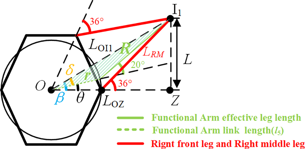
As depicted in Figure 7, taking the RM + RH failure as an example, the front extreme position I
1 of the FA foot-end corresponds to the intersection point achieved when the RF swings backwards to its maximum angle (−36°) and the RM swings forward to its maximum angle (36°). The angle
 $ \beta$
between the line connecting point O and point I
1 and the transverse axis of the body is calculated from Eq. (6) to be approximately 24°.
Calculation of the compensation median angle θ.

Figure 7 Long description
A diagram of the gait replanning for a hexapod robot experiencing the loss of a single leg. The diagram includes various labeled components and angles that describe the robot's movement and stability. Key elements include the functional arm effective leg length, functional arm link length, and the right front leg and right middle leg. The diagram shows the relationships between these components, with specific angles and distances marked. The functional arm effective leg length is depicted in green, the functional arm link length in dashed green, and the right front leg and right middle leg in red. Angles such as 36 degrees and 20 degrees are indicated, along with distances labeled as L, LO11, LZ, and LRM. The diagram also includes a central point labeled O and various other points and lines that contribute to the overall structure and movement of the robot.
 \begin{align} L&=L_{\rm RM}\sin 36^{\circ} \\[-8pt] \nonumber \end{align}
 \begin{align} L_{\rm OZ}&=L_{\rm RM}\cos 36^{\circ}+r \\[-8pt] \nonumber \end{align}
 \begin{align} \beta &=\arctan \frac{L_{\rm RM}\sin 36^{\circ}}{L_{\rm RM}\cos 36^{\circ}+r} \\[8pt] \nonumber \end{align}
In Eq. (5), LRM represents the effective leg length of the mechanical leg, and LOZ denotes the distance between point O and point Z.
The position I
1 corresponds to a swing angle
 $ \alpha$
of 20°, as indicated by the green-shaded triangle in Figure 7. The value of δ is calculated using Eq. (7), and the angle θ corresponding to the foot-end position I
1 is then calculated using Eq. (8) to be approximately 9.6°.
 \begin{align} L_{{\rm O}{{\rm I}_{1}}}&=\sqrt{R^{2}+{r}^{2}-2R\text{rcos}(180^{\circ }-\alpha )} \\[-8pt] \nonumber \end{align}
 \begin{align} \delta &=\arccos \frac{{L_{{O}{{ I}_{1}}}}^{2}+r^{2}-R^{2}}{2L_{{ O}{{ I}_{1}}}r} \\[-8pt] \nonumber \end{align}
 \begin{align} \theta &=\beta -\delta \\[10pt] \nonumber\end{align}
For determining the I
2 position (Figure 6(a)), the location of foot-end A must be taken into account. When the FA foot-end is located at point I
2, point O lies on the line segment connecting I
2 and A at the boundary of the support polygon. This configuration corresponds to a critically unstable state, in which the allowable range of θ is maximized. By setting the swing angle
 $ \alpha$
to its minimum value of −20°, the minimum θ value for the I
2 position is determined to be −40°.
3.3.4. Calculation of longitudinal stability margin S
Let the coordinates of point A be (x
a
, y
a
), point C be (x
c
, y
c
), and point J be (x
j
, y
j
). The slope k
2 of line JA is determined by:
 $\mathit{k}_{2}\mathit{=}\frac{\mathit{x}_{\mathit{j}}\mathit{-}\mathit{x}_{\mathit{a}}}{\mathit{y}_{\mathit{j}}\mathit{-}\mathit{y}_{\mathit{a}}}$
, then the equation of line JA is:
 \begin{equation} y_{ JA}-y_{a}=k_{2}(x_{ JA}-x_{a}) \end{equation}
Similarly, the slope k
1 of line JC is:
 $\mathit{k}_{1}\mathit{=}\frac{\mathit{x}_{\mathit{j}}\mathit{-}\mathit{x}_{\mathit{c}}}{\mathit{y}_{\mathit{j}}\mathit{-}\mathit{y}_{\mathit{c}}}$
, the equation of line JC is:
 \begin{equation} y_{ JC}-y_{c}=k_{1}(x_{ JC}-x_{c}) \end{equation}
Based on the longitudinal stability margin, the distance from O to line AJ is denoted as l OE, and the distance from O to line CJ is denoted as l OF, as shown in Figure 6. Setting the x-intercepts of lines JC and JA to zero (x JC = 0, x JA = 0) and solving the simultaneous Eqs. (9) and (10) yields the values l OE and l OF as:
 \begin{align} l_{ OE}=\left| -x_{a}k_{1}+y_{a}\right| \\[-8pt] \nonumber \end{align}
 \begin{align} l_{OF}=\left| -x_{c}k_{2}+y_{c}\right| \\[12pt] \nonumber \end{align}
The longitudinal stability margin S is then defined as the minimum value between l OE and l OF as:
 \begin{equation} S=\min \{l_{OE},l_{OF}\} \end{equation}
3.3.5. Global optimization of gait sequences and compensatory positions
Taking the RM + RH failure as an example, the robot reaches a critically unstable state when the RF is in the swing phase with its foot-end located at the front extreme position (front 2). Under this critical condition, compensatory motion by the FA achieves maximum effectiveness. As shown in Figure 3, the robot adopts a wave gait in which each leg contacts the ground at five discrete foothold positions during one gait cycle. Although the state of the RF is known, the states of the other legs (LF, LM, LH, FA) are undetermined, and the overall gait sequence remains unspecified. Therefore, the foot-end positions for LF, LM, LH, and FA must be selected from the front 1, median, hind 1, and hind 2 positions, yielding 24 possible position combinations. The developed optimization algorithm iterates over θ and α for each gait sequence to calculate the stability margin S. In the implementation, the search was performed as an exhaustive grid scan. Specifically, the swing angle α was discretised into five candidate values, corresponding to representative foothold positions within the foot’s available workspace: −20°, −10°, 0°, 10°, and 20°. The compensation median angle θ was swept across its feasible range with a step size of 0.001°. On a standard desktop MATLAB platform, the average runtime for a single failure case was approximately 30 min. Since this optimization is carried out offline to precompute the optimal compensatory gait sequence and foothold configuration, its computational cost does not affect the real-time execution of the feedforward walking controller.
4. Theoretical analyses of FA compensation results
4.1. Determination of the θ range
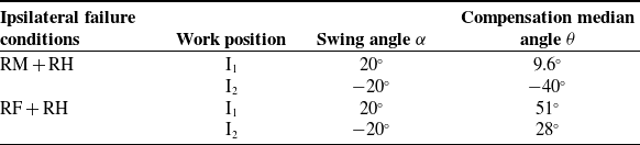
The range of the compensatory median angle θ for FA is constrained by the boundaries I 1 and I 2, as outlined in Section 3. In the case of an RM + RH failure, I 1 is constrained by the maximum swing angle of the RF leg due to interference limitations, while I 2 is defined by the position A of the LF foot-end and the critically unstable state of the robot. The process for determining the values of α and θ is detailed in Section 3, and the resulting values are provided in Table III. Similarly, for RF + RH failure, the determination of I 1 must account for the position of point C. When the FA foot-end is at I 1, point O lies on the line connecting I 1 and C along the support polygon boundary, placing the robot in a critically unstable state. Here, with α = 20°, the corresponding θ is 51°. On the other hand, I 2 is constrained by the maximum swing angles of two legs. The position of I 2 is identified when the line connecting O and I 2 is on the verge of interfering with the RM. At this position, with α = −20°, the value of θ is 28°. The values of α and θ under FA compensation for both failure scenarios are summarized in Table III.
α and θ under FA compensation.

Table III Long description
A table titled 'Table III. and under FA compensation.' presents data on compensation median angles under ipsilateral failure conditions. The table has four rows and three columns. The columns are labeled 'Ipsilateral failure conditions,' 'Work position,' 'Swing angle α,' and 'Compensation median angle θ.' The row labels under 'Ipsilateral failure conditions' are 'RM + RH' and 'RF + RH.' For 'RM + RH,' the work positions are 'I1' and 'I2' with swing angles of 20 degrees and -20 degrees, and compensation median angles of 9.6 degrees and -40 degrees, respectively. For 'RF + RH,' the work positions are 'I1' and 'I2' with swing angles of 20 degrees and -20 degrees, and compensation median angles of 51 degrees and 28 degrees, respectively.
Stability margin of different gait sequences. (a) RM + RH failure. (b) RF + RH failure.

Figure 8 Long description
Two line graphs depict stability margins for different gait sequences in hexapod robots experiencing leg failures. Panel A: The line graph shows the stability margin S in centimeters on the vertical axis and the compensatory median angle θ in degrees on the horizontal axis. The graph includes multiple lines representing different gait sequences, each identified by a unique number and color. The stability margin increases with the compensatory median angle, with some lines showing steeper increases than others. Panel B: The line graph shows the stability margin S in centimeters on the vertical axis and the compensation median angle θ in degrees on the horizontal axis. Similar to Panel A, multiple lines represent different gait sequences, each identified by a unique number and color. The stability margin decreases with the compensation median angle, with some lines showing steeper decreases than others. Both graphs illustrate how different gait sequences affect the stability margin of hexapod robots under specific leg failure conditions.
4.2. Gait sequence and stability margin
Figure 8 shows the stability margin S values for 24 gait sequence combinations under different θ angles during ipsilateral two-leg failure with FA compensation. For the RM + RH failure (Figure 8(a)), S increases monotonically with θ and reaches its maximum value S = 26.3 cm at the inflection point θ = 5.7°. In the case of RF + RH failure (Figure 8(b)), S generally decreases as θ increases, attaining the maximum stability margin S = 24.3 cm at the boundary θ = 28°. A comparison shows that the S-θ curve for the RF + RH failure changes more gradually, indicating that the stability margin is less sensitive to changes in θ under this condition than under the RM + RH failure. Furthermore, under both failure modes, the curve corresponding to the optimal gait sequence not only achieves the best performance at the extreme points but also maintains the highest stability margin across the entire range of θ, demonstrating that the optimal gait sequence possesses strong robustness and resistance to angular disturbances.
The corresponding optimal gait sequences are shown in Figure 9, for RM + RH failure (Figure 9(a)), the sequence is RF→LH→LM→FA→LF; for RF + RH failure (Figure 9(b)), the sequence is RM→LH→LM→FA→LF. Each leg state is labeled in the form X(Y), where X represents the leg identifier, and Y denotes the associated gait phase number. The diagrams below (a–e), which mark the stepping sequence, visually demonstrate that at every time step of the gait cycle, the projected COG remains safely inside the reconstructed support triangle formed by the FA and remaining legs, confirming continuous static stability.
Optimal gait sequences and movement state for FA compensation. (a) RM + RH failure. (b) RF + RH failure.

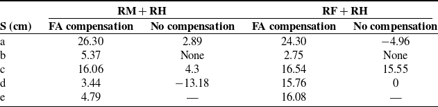
The stability data in Table IV confirm the effectiveness of the FA compensation strategy. Under the optimal compensated gait sequences, the robot maintains a positive stability margin (S) throughout the entire gait cycle, eliminating the unstable state caused by ipsilateral two-leg failure and restoring continuous, stable walking.
Stability margin throughout a full gait cycle.

Table IV Long description
The table presents stability margins throughout a full gait cycle for different robot configurations and compensation strategies. It has five rows and four columns. The columns are labeled RM + RH FA compensation, RM + RH No compensation, RF + RH FA compensation, and RF + RH No compensation. The rows are labeled with different gait phases: a, b, c, d, and e. Each cell contains a numerical value representing the stability margin in centimeters. Notable values include positive margins indicating stable states and negative values indicating unstable states. The table also notes that 'None' indicates that the support polygon does not intersect the longitudinal axis, making the longitudinal stability margin incalculable, and that certain gait phases do not exist in the four-legged wave gait without FA compensation.
Note: “None” indicates that the support polygon does not intersect the longitudinal axis, making the longitudinal stability margin incalculable; “—” denotes that this particular gait phase does not exist in the four-legged wave gait without FA compensation. Negative values indicate an unstable state.
5. Experiment and results analysis
5.1. Prototype experiment platform
Built upon the SpiderPi hexapod robotics platform, we developed custom mounting components to install the FA system at the centroid-symmetric location of the chassis. The overall hardware architecture and experimental setup are illustrated in Figure 10. The experimental system uses a Raspberry Pi 3B+ as the main controller, which supports remote communication via the VNC protocol. An LSC-20-U1.3 servo control board was used to drive 18 LDX-218 digital servos. Gait execution was implemented in a feedforward manner through the Raspberry Pi 3B+ and the servo controller, with a command update interval of 1 ms. An MPU6050 IMU was used to measure the robot’s real-time roll and pitch angles, with an angular measurement uncertainty of ±0.3°. Before attitude evaluation, the raw IMU data were filtered using a Kalman filter, with parameters set to Q angle = 0.001, Q bias = 0.003, R measure = 0.03. Walking tests were conducted on a flat ground surface equipped with fiducial markers to track foot-end displacements under different gait patterns, with a displacement measurement uncertainty of ±0.5 cm. Each experimental condition was repeated for five trials, and one complete gait cycle was recorded in each trial. In the wave-gait framework adopted in this study, one gait cycle was defined as the full locomotion sequence from the initial phase to the completion of all gait phases. Each gait phase lasted 0.8 s, resulting in a total cycle duration of 4 s. The filtered IMU signals were used to obtain roll and pitch angles over the normalized gait cycle, while the marker-based tracking results were used to extract displacement data for comparative analysis.
Hardware system and experimental platform for the FA hexapod robot.

5.2. Validation of FA compensation test
5.2.1. Walking stability
For the RM + RH failure (Figure 11) without FA compensation, the robot initially maintains a stable posture (a1). However, when the RF enters the swing phase (b1), the loss of support on the right side causes the COG to shift rightward, and the robot begins to roll. As the LH subsequently swings (d1), the loss of posterior-right support further destabilizes the robot, resulting in a compound overturning moment that leads to rollover instability on the rear-right side. In contrast, with FA compensation (states a2−e2), the COG remains consistently within the support polygon throughout the entire gait cycle, enabling stable locomotion. The measured stability margin in the physical experiment matches closely with theoretical predictions, with errors within ±3 cm.
Locomotion test with/without FA compensation under RM + RH failure.

Figure 11 Long description
The image consists of multiple photos and diagrams showing a hexapod robot's movement patterns and stability margins during leg failure scenarios. The photos and diagrams are arranged in a grid format with two rows and five columns, each labeled with different time stamps and stability margin values. Panel A1: A photo of a hexapod robot with labels indicating the positions of its legs (LF, RF, LM, LB, FA). The robot is in a stable position with all legs extended. Panel A2: A diagram of the same robot with red dashed lines indicating the stability margins. The stability margin value is 26.9. Panel B1: A photo of the robot in a different position, with legs adjusted to compensate for a failure. Panel B2: A diagram showing the stability margins with a value of 3.42. Panel C1: A photo of the robot in another adjusted position. Panel C2: A diagram showing the stability margins with a value of 19.36. Panel D1: A photo of the robot in yet another adjusted position. Panel D2: A diagram showing the stability margins with a value of 3.52. Panel E1: A photo of the robot in a final adjusted position. Panel E2: A diagram showing the stability margins with a value of 3.09. The diagrams illustrate the robot's ability to maintain stability despite leg failures by adjusting its gait and leg positions. The stability margins are calculated and displayed to show the robot's stability in different scenarios.
For the RF + RH failure (Figure 12), the system without FA compensation exhibits an initial loss of frontal support during the LF swing phase (a3), leading to forward inclined tipping tendency. Subsequent RM swing phase (b3) further reduces support on the right flank, amplifying the roll instability. Pronounced displacement of the COG eventually results in critical instability and rollover. With FA compensation applied (a4−e4), the COG remains effectively constrained within the support polygon throughout all gait phases, consistently maintaining full stability. As with the RM + RH failure case, the measured stability margin shows close agreement with theoretical values, with a deviation within ±3 cm.
Locomotion test with/without FA compensation under RF + RH failure.

5.2.2. Attitude angle analysis
A comparative analysis of attitude angle dynamics under RM + RH and RF + RH failure conditions demonstrates substantial improvements with FA compensation, as shown in Figures 13 and 14. The shaded error bands represent the mean ± SD deviation from five repeated trials, which quantitatively illustrate the variability in roll and pitch responses with and without FA compensation. Without FA compensation, during RM + RH failure, the roll angle fluctuates within [−13°, 5°] and the pitch angle within [−1°, 9°], correlating directly with instability during the swing phases of the RF and LH (Figure 11). Similarly, for RF + RH failure without compensation, the roll angle fluctuates within [−15°, 7.5°] and the pitch angle within [−2°, 10°], with the most severe oscillations occurring in the first half of the cycle (T = 0–1/2). With FA compensation, the roll and pitch angles are significantly stabilized. For RM + RH failure, the roll and pitch angles are reduced to [–2.5°, 1°] and [–2.5°, 0°], respectively. In the case of RF + RH failure, the roll angle remains around –2.5° and the pitch near –3°, both with minimal variation. These results confirm that FA compensation effectively suppresses multidirectional instability and significantly enhances locomotion smoothness.
Roll and pitch angle comparison under RM + RH failure.

Figure 13 Long description
The image contains two line graphs labeled Panel A and Panel B, comparing roll and pitch angles under RM + RH failure conditions with and without FA. Panel A: This line graph shows the roll angle in degrees on the vertical axis and the cycle in terms of T on the horizontal axis. The graph compares two conditions: with FA (black line) and without FA (red line). The shaded areas around the lines represent the variability or confidence intervals. The roll angle fluctuates between -20 and 10 degrees over the cycle, with notable dips and peaks at specific intervals marked by dashed vertical lines. Panel B: This line graph displays the pitch angle in degrees on the vertical axis and the cycle in terms of T on the horizontal axis. Similar to Panel A, it compares conditions with FA (black line) and without FA (red line), with shaded areas indicating variability. The pitch angle ranges from -4 to 12 degrees, showing distinct peaks and troughs at intervals marked by dashed vertical lines. The graphs illustrate how the presence or absence of FA affects the roll and pitch angles during the cycle, highlighting differences in stability and control under failure conditions.
Roll and pitch angle comparison under RF + RH failure.

5.2.3. Foot-end displacement analysis
As shown in Figure 15, a comparative analysis of foot-end displacements under the ipsilateral two-leg failure condition demonstrates significant locomotion enhancement with FA compensation. For RM + RH failure, the uncompensated gait shows only 1.5 cm mean displacement per cycle, indicating severely limited mobility. With FA compensation, this value increases to 11 cm – a 7-fold improvement. For RF + RH failure, the average displacement without compensation was 3 cm, largely due to instability-induced gait switching. With compensation, it rose to 8 cm – a 2.7-fold improvement. Furthermore, the use of FA compensation leads to a more uniform displacement distribution and improved consistency in the foot-end trajectory.
Foot-end displacement comparison under ipsilateral two-leg failure.

Figure 15 Long description
The image contains multiple photos and diagrams illustrating the effects of single-leg failures in quadruped robots and the methods used to mitigate these failures. The photos and diagrams are arranged in a grid format with labels indicating different failure scenarios and compensation methods. Panel A: A photo showing a quadruped robot with a failure in the right middle and right hind legs. The left front leg is extended forward, and a ruler is placed next to the leg to measure displacement. Panel B: A photo showing a quadruped robot with a failure in the right middle and right hind legs, with fault tolerance compensation applied. The left front leg is extended forward, and a ruler is placed next to the leg to measure displacement. Panel C: A photo showing a quadruped robot with a failure in the right front and right hind legs. The left front leg is extended forward, and a ruler is placed next to the leg to measure displacement. Panel D: A photo showing a quadruped robot with a failure in the right front and right hind legs, with fault tolerance compensation applied. The left front leg is extended forward, and a ruler is placed next to the leg to measure displacement. Panel E: A photo showing a quadruped robot with a failure in the front auxiliary leg. The left front leg is extended forward, and a ruler is placed next to the leg to measure displacement. Panel F: A photo showing a quadruped robot with a failure in the right middle and right hind legs, with fault tolerance compensation applied. The left front leg is extended forward, and a ruler is placed next to the leg to measure displacement. Panel G: A photo showing a quadruped robot with a failure in the right front and right hind legs. The left front leg is extended forward, and a ruler is placed next to the leg to measure displacement. Panel H: A photo showing a quadruped robot with a failure in the right front and right hind legs, with fault tolerance compensation applied. The left front leg is extended forward, and a ruler is placed next to the leg to measure displacement. Panel I: A photo showing a quadruped robot with a failure in the front auxiliary leg. The left front leg is extended forward, and a ruler is placed next to the leg to measure displacement.
Figure 16 presents the foot-end displacement under ipsilateral two-leg failure, with error bars indicating the mean ± SD deviation. Statistical data from five repeated trials confirm that under RM + RH failure, FA compensation simultaneously increases the mean displacement and reduces the standard deviation, indicating improved motion consistency. Similarly, for RF + RH failure, a comparable increase in mean displacement accompanied by enhanced stability is observed. Asterisks indicate statistically significant differences between the “With FA” and “Without FA” conditions for the same leg, as determined by paired t-tests (n = 5, *** p < 0.001).
Comparison of foot-end displacement for ipsilateral two-leg failure. (a) RM + RH failure; (b) RF + RH failure.

6. Discussion
FT strategies for multi-legged robots differ substantially in recovery capability, stability enhancement, computational load, and implementation complexity. Conventional gait-reconfiguration methods are computationally efficient, but they are mainly suitable for single-leg or relatively moderate fault cases. Model- or planning-based methods can address more complex faults, yet they often require higher implementation complexity and computational cost. Learning-based approaches have shown strong adaptability in fault recovery, but they are generally training-dependent and may face challenges in real-world deployment.
In contrast, the proposed FA compensation strategy is designed for bilaterally symmetric hexapod robots suffering from ipsilateral two-leg failure. By introducing the FA as an additional support point at the robot center, the method directly reconstructs the support polygon, repositions the COG within the stable region, and enhances resistance to overturning. Moreover, the strategy is based on offline parameter optimization, avoiding high-dimensional gait search and real-time force control. As a result, it improves the longitudinal stability margin and stride while maintaining low computational load and good engineering feasibility. With further integration of gait pre-adjustment, mechanical reinforcement, drive optimization, and online perception/planning, the proposed framework may be extended to heavy-load and unstructured-terrain applications.
Although the results demonstrate the feasibility of the proposed strategy, several limitations of the present study should be acknowledged. First, the proposed strategy was developed and validated only under flat-terrain conditions. Second, both the analysis and the experiments were limited to quasi-static straight walking, and the applicability of the proposed strategy to turning, lateral movement, or more complex actions remains to be investigated. Third, this study focused on feedforward control, which still needs to be integrated with real-time control for locomotion on rough terrain, dynamic walking, and more complex motion tasks.
7. Conclusions and prospect
This paper has presented an FA compensation strategy for recovering locomotion in hexapod robots under ipsilateral two-leg failures (RM + RH and RF + RH). By maximizing the longitudinal stability margin (S), the compensatory median angle θ and swing angle α of the FA were optimized to determine the optimal foot-end position and gait sequence. The proposed approach ensures that the minimum stability margin remains positive throughout the entire gait cycle for both failure scenarios, thereby maintaining the COG within the support polygon. Experimental validation demonstrated significant performance improvements. For RM + RH failure, the roll and pitch angles were reduced from [–13°, 5°] and [–1°, 9°] to [–2.5°, 1°] and [–2.5°, 0°], respectively, while the mean foot-end displacement increased sevenfold to 11 cm. Under RF + RH failure, the roll and pitch angles stabilized around –2.5° and –3°, respectively, with a twofold increase in mean foot-end displacement to 8 cm. These results demonstrate that the proposed FT compensation strategy effectively restores the robot’s locomotion capabilities, providing a viable feedforward control solution for the sustained and reliable operation of multi-legged robots under severe leg damage.
Leveraging the low computational overhead of the feedforward gait control strategy developed in this study, it can be further integrated with posture and terrain perception to enable rapid recovery under high damage conditions and adaptive adjustments during walking. It can also be extended to more complex scenarios, such as slopes, rugged terrain, turning maneuvers, and varying-friction conditions, to enhance environmental adaptability. Future research will further investigate FT walking strategies under a wider range of damage conditions, including joint locking, partial leg loss, and cases in which damaged legs remain attached to the torso. In addition, arm-contact force measurement or more detailed load calibration would provide a more direct evaluation of the compensation mechanism. In the future, integrating the proposed feedforward gait generation framework with reinforcement-learning-based adaptive control represents an important direction for the next stage of this research.
Author contribution
All authors made substantial contributions to this work. Chenxu Lu designed the experimental scheme and wrote the first draft. Hu Zhang analyzed the experimental results. Yan Zhang contributed to writing–review and editing, supervision, and conceptualization. Yuhe Guo conducted data collection. Xinghua Lin and Hao Wang performed the statistical analyses.
Financial support
This work was supported by the National Natural Science Foundation of China (Grant Nos. 51405341, 62403356, 62301360). The Youth Project of Tianjin Natural Science Foundation (No.25JCQNJC01070).
Conflicts of interest
The authors declare no conflicts of interest exist.
Ethical approval
Not applicable.