INTRODUCTION
A mainstay of much ecological community work, and particularly biologically-based studies of environmental impact, is multivariate analysis of assemblage matrices. Here, we shall adopt the convention that the matrix columns represent n independent samples (of water, sediment, reefs, shores, soil, vegetation transects, etc.) and its rows the suite of p taxa or OTUs (hereafter ‘species’) identified in those samples. Matrix entries are species counts or density, biomass, area cover, etc. (hereafter ‘abundance’, where finer distinction is unnecessary). The data analyst is always faced, however, with an initial decision on pre-treatment of the data prior to synthesizing the relationships between samples, from essentially n points in p dimensional space, into n(n-1)/2 pairwise distances, similarities or dissimilarities (hereafter ‘resemblances’) between samples, using an appropriately chosen resemblance measure. This triangular resemblance matrix is the starting point for a wide range of multivariate analyses, whether hierarchical clustering (agglomerative or divisive), ordination by principal coordinates (PCO) or non-metric multi-dimensional scaling (MDS), hypothesis testing by permutations of the resemblance structure, and so on (e.g. Clarke, Reference Clarke1993; McArdle & Anderson, Reference McArdle and Anderson2001).
Much has been written about directed choice of resemblance measure to capture certain important properties of the data structure (e.g. Faith et al., Reference Faith, Minchin and Belbin1987; Legendre & Legendre, Reference Legendre and Legendre1998; Clarke et al., Reference Clarke, Somerfield and Chapman2006b) but rather less about directed choice for pre-treatment of the data matrix, by some form of transformation or differential species weighting, prior to calculation of resemblances. Clearly, care must be exercised when dealing with a single data set not to explore large numbers of such analysis choices, selecting only those which result in confirmation of a priori prejudices about what story the data should tell! If multiple analyses are performed, multiple results should be presented, allowing the reader properly to judge the dangers of selection bias in interpreting only the ‘best’ outcomes. Of greatest importance, however, is to learn the lessons from the current analysis about good long-term choice of a suitable sequence of pre-treatment steps, to apply routinely to future studies of comparable groups of biota under similar scenarios for hypothesis-testing and subsequent interpretation. It is in this context that we present the use of ‘shade plots’ as an effective tool for examining the likely outcomes from the range of pre-treatment options now discussed.
Some resemblance measures automatically weight species by standardizing their abundances across samples to a fixed total, maximum or range, as in the quantitative form of Gower's similarity coefficient (Gower, Reference Gower1971). This effectively gives each species equal weight in the ensuing calculations, irrespective of its total abundance or frequency of occurrence. However, for the widely-used Bray–Curtis dissimilarity measure (Bray & Curtis, Reference Bray and Curtis1957), species are given an emphasis that is very much determined by their maximum abundance across samples. The same is true of many of the related, biologically-oriented measures, which Clarke et al. (Reference Clarke, Somerfield and Chapman2006b) termed members of the ‘Bray–Curtis family’. It has long been recognized, therefore, that some form of overall transformation of abundances is usually necessary prior to computation of such biological similarities, in order that more than just the few most dominant species play some role in defining among-sample resemblances. Clarke & Green (Reference Clarke and Green1988) is commonly cited as a reference for the relative effects of different transformations on community analyses, but the need for transformation of species data had been well-understood in earlier decades (e.g. Clifford & Stephenson, Reference Clifford and Stephenson1975) and its role in univariate statistics extensively researched (e.g. Box & Cox, Reference Box and Cox1964).
In the multivariate case, Olsgard et al. (Reference Olsgard, Somerfield and Carr1997, Reference Olsgard, Somerfield and Carr1998) and Olsgard & Somerfield (Reference Olsgard and Somerfield2000) presented an indirect methodology for assessing the relative effects of choice of transformation on the among-sample pattern. This used ideas of similarity in the rank order pattern of resemblance matrices calculated under different transformation choices, then viewed in second-stage MDS plots (Somerfield & Clarke, Reference Somerfield and Clarke1995). Clarke et al. (Reference Clarke, Somerfield and Chapman2006b) described one way of potentially selecting a ‘best’ transformation for future use, where there are a priori defined groups of samples, e.g. of sites, times or treatments. This uses the ANOSIM R statistic (Clarke & Green, Reference Clarke and Green1988), which contrasts the average of the rank dissimilarities among groups to those within groups and thus measures the degree of separation of the groups in multivariate space. One important feature of the non-parametric ANOSIM test, not shared by most other multivariate testing procedures, is the lack of dependence of its test statistic (R) on the specific measurement scale of the resemblances. Thus, values of R can be compared across different transformation choices for pre-treatment of the raw data, prior to resemblance calculation, and the transformation maximizing R might be considered a good candidate for use with further data collected in this particular context. It is important here to re-iterate the dangers of selection bias: the same data cannot be used to select an optimum transformation and also validate its likely performance in future!
Under an alternative scenario in which the interest is in optimizing the link between the biological assemblages and potentially forcing environmental variables, the choice of initial transformation of the biotic matrix might seek to optimize the maximal ρ statistic from the BEST (Bio-Env) procedure (Clarke & Ainsworth, Reference Clarke and Ainsworth1993). Here ρ is a non-parametric form of the Mantel statistic (Mantel, Reference Mantel1967) capturing the match of biotic and environmental resemblances, again in a scale-independent way. Such an approach was taken by Olsgard et al. (Reference Olsgard, Somerfield and Carr1997) in the context of describing changes to benthic macroinvertebrate communities, correlatively linked to a suite of sediment contaminant variables sampled at the same set of sites positioned at different distances from a North Sea oil-field.
In the above-mentioned approaches, however, the assessment of what constitutes a ‘good’ transformation is one-step removed from the data matrix itself, since they are characterized by relationships involving only the resulting resemblance matrices. A different approach to pre-treatment is a differential rescaling of variables (species), thus changing the relative weighting that each species gets in the calculation of sample resemblances. One simple form of this is the species standardization implicit in Gower's coefficient, in which all species are potentially given the same weight. More effective possibilities include: (a) down-weighting species in proportion to the extent to which they are misidentified (Mumby et al., Reference Mumby, Clarke and Harborne1996); (b) rescaling variables by standard deviation (SD) weighting, i.e. computing the SD of that variable within a priori-defined groups, averaging those SDs across the groups and dividing the variable by this average SD (Hallett et al., Reference Hallett, Valesini and Clarke2012); and (c) dispersion weighting (DW, Valesini et al., Reference Valesini, Potter and Clarke2004; Clarke et al., Reference Clarke, Chapman, Somerfield and Needham2006a), in which the differing degree to which species form spatial clumps in the environment is explicitly recognized and estimated. Specifically, DW calculates for each species, over replicate samples within prior-defined groups, the index of dispersion of its abundances (D = variance/mean), averages D over the groups to give  $\overline{D}$, then divides that species' abundances through by $\overline{D}$. This procedure can be formally justified under rather weak model assumptions, namely that the integer counts for a species to follow a generalized Poisson model. This postulates centres of its population (the clumps) distributed spatially at random, with differing densities of centres in different groups, and a randomly variable number of individuals associated with each centre. This clump size is of an unspecified distributional form, which may vary from species to species but, within a species, its mean and variance are assumed constant across groups. In other words, different sites, times, impacts, etc. may change the density of clumps but not the average (or variance in) size of a clump. This semi-parametric generalized Poisson model subsumes many commonly used distributions for species counts (see Clarke et al., Reference Clarke, Chapman, Somerfield and Needham2006a), one special case being the fully parametric negative binomial model, recently advocated by Warton et al. (Reference Warton, Wright and Wang2012) as a way of accommodating variance–mean relationships commonly found in matrices of species counts. Dispersion weighting therefore more generally corrects for such variance–mean relationships, species by species, having the effect of relativizing all species to the same Poisson-like structure of variance equal to the mean, within groups. A simple (somewhat over-simple) way of conceptualizing this is that the dispersion-weighted data matrix now records for each species the number of clumps captured, rather than individuals captured, thus removing the dominant effects of species with large counts which are highly erratic among replicates of the same condition, and therefore leading to more robust multivariate analyses. Thus, unlike the Warton et al. (Reference Warton, Wright and Wang2012) approach (which could be seen as ‘throwing the baby out with the bathwater’), it is not necessary to forgo the many advantages of working with resemblance matrices which are not Euclidean (e.g. recognizing the special role of zeros in the data matrix, as in the issue of interpreting ‘joint absences’, Clarke et al., Reference Clarke, Somerfield and Chapman2006b), simply in order to adjust for differing variance–mean ratios among species.
In their formulation of DW, however, Clarke et al. (Reference Clarke, Chapman, Somerfield and Needham2006a) identified the possibility that, having put all species counts onto a consistent footing, there might still be a case for mildly transforming the dispersion-weighted matrix, e.g. with a square-root transformation. This would down-weight the contributions of consistently high-abundance species (over replicates within a group) in relation to consistently low-abundance species. In other words, one of the reasons for the use of severe transformations such as log(1 + x) or x 0.25, namely to down-weight species with erratic counts over replicates, will have been removed by dispersion weighting, but the other major reason may still remain. That is, resemblances will need to be computed from a balance of contributions of abundant, less dominant and rare species, as called for by the specific context and hypotheses of interest (Clarke & Warwick, Reference Clarke and Warwick2001: ch. 2). It is interesting to note though, that most users of the DW technique to date have tended not to follow DW by any form of overall transformation, and (whether the data has been initially dispersion-weighted or not) the choice of overall transformation, to best capture the spread of contributions from across the assemblage in the resemblance computations, has always been something of a ‘stab in the dark’ for many ecologists carrying out multivariate analyses. One indication of this was an informal study (by the first author) of papers employing earlier versions of the PRIMER software. This demonstrated that when the default transformation in the package was fourth-root, most users employed fourth-root transforms in their studies, and when the default switched to square-root, for later versions of the software, users predominantly moved to square-root transformations! Thus, whilst the motivation for employing different transformations may now be well understood (e.g. that studies of impact on biodiversity, which are primarily interested in detecting changes to a wide range of species, should utilize heavier transformations than ecosystem-focused studies, which are more concerned with the abundance or biomass dominants in the assemblage), in practice the tools available to help the user gauge the effects of differing-strength transformations on the data matrix, in bringing into reckoning a greater or lesser number of species, have been inadequate.
The present paper, therefore, simply suggests that directly viewing the (possibly pre-treated) values in the data matrix, which are about to enter into the calculation of resemblances, is highly informative in deciding whether the right balance across species has been struck for the specific context and hypotheses of interest. When there are many samples and species, however, viewing the data table itself can be difficult, especially for non-integral numbers arising from biomass, area cover etc. This can be further exacerbated by the occasional presence of exponential notation for small numbers, perhaps resulting from density calculations or dispersion weighting. People are simply not good at assimilating broad trends from information presented in large tables. Graphical representation, however, is another matter: presenting the matrix in the form of a simple ‘shade plot’, in which the larger the (pre-treated) abundance the darker is the shade of the rectangle corresponding to that particular combination of sample and species, gives a visual display which is at once direct, relevant, simply interpretable and capable of carrying powerful messages about the effects that different choices of transformation (with or without prior DW) will have on subsequent multivariate analyses.
The purpose of this paper is, therefore, to present a general exposition of a simple method for visualizing the effects of different data pre-treatments, applicable to all community studies, by using two specific data sets purely as illustrations of the issues involved.
MATERIALS AND METHODS
Example data sets
The following recently completed studies of faunal groups in Western Australian estuaries are used to demonstrate choice of transformation (including reduction to frequency of occurrence of species) on a raw data matrix, and the possible need for transformation following dispersion weighting (DW).
UPPER SWAN ESTUARY MACROBENTHOS
Assemblages of benthic macroinvertebrates (hereafter ‘macrobenthos’) in the sediment of five locations in the upper Swan Estuary, Perth, Western Australia, were sampled 12 times over the period January 2010–October 2011, on each occasion taking five Ekman grab samples at each location, giving a total of 300 samples (Tweedley & Hallett, Reference Tweedley and Hallett2013). The sampling times were monthly between January and July 2010, and thereafter quarterly, in October 2010, January, April, July and October 2011. Each Ekman grab collected sediment from an area of 225 cm2 and to a depth of 15 cm, which was then sieved through a 500 μm mesh. The counts made of organisms from the three main phyla or sub-phyla (Annelida, Mollusca and Crustacea), many of them identified to species level, are used for this illustration. The 35 taxa identified in these three groups constituted 99.7% of all organisms counted.
The main interest in this data set is that it was collected over a period which included a major weather event in the Perth region (22 March 2010, between sampling time points 3 and 4). An intense storm passed directly over the area, causing a costly natural disaster estimated at >A$1b, and impacting much of the metropolitan zone (Buckley et al., Reference Buckley, Sullivan, Chan and Leplastrier2010). The extensive hail and 44 mm of heavy rain, which fell in half an hour, was the first rainfall in the region for four months, and the interest was, therefore, in establishing whether the resulting flash floods left a detectable signal in the macrobenthic community of the upper Swan Estuary in the ensuing months. The possible mechanisms for anticipating such a signal, and interpretation of the nature of any changes detected, are given in Tweedley & Hallett (Reference Tweedley and Hallett2013). The motivation in the present paper is simply to explore the effect of different options for data pre-treatment on the ability to detect such a signal, and thus demonstrate the general role shade plots can play in visualizing the effects of different transformations and species weightings on the ensuing analyses.
Whilst the replicate grab samples can play a useful part in hypothesis testing for specific differences between sampling occasions at a particular location, or of differences between locations at a specific time, their primary role here is in providing a sound estimate of community composition at these five locations over the time course of sampling, to better display the patterns of assemblage change that may have resulted from this major disturbance. In that context, it is appropriate to average over the replicates in some way. In multivariate studies, just as in univariate ones, averaging is often best carried out after any transformation of the original data values. So, here we generate a number of alternative pre-treated data matrices at the replicate level, which after averaging could be input to resemblance calculations, and which span the gamut of contributions drawn from numerically dominant species to infrequently occurring ones. Transformation options used on the original replicate counts are: untransformed, square-root, fourth-root and reduction to presence/absence, with the transformed data then averaged over the replicates for each of 60 sets, namely all combinations of times (1–12) and locations (1–5). Note that, for the last of these transformation choices, averaging over replicate samples that have been reduced to presence or absence (1 or 0) turns the matrix entry into a relative frequency of occurrence of each species at each combination of time and location, taking values on a six-point scale: 0, 0.2, 0.4, 0.6, 0.8, 1. Such frequency-based information, where replication of samples at a low level allows it to be obtained, can be an effective way of generating data which are statistically ‘well-behaved’ from counts which can be extremely erratic (right-skewed) in distribution.
A further pre-treatment option considered here is that of dispersion weighting. Separately for each species, this down-weights all replicates by $\overline{D}$, the variance-to-mean ratio D of counts for each set of five replicates, averaged over the 60 combinations of time and location (excluding sets in which no individuals of that species are found, Clarke et al., Reference Clarke, Chapman, Somerfield and Needham2006a). These dispersion-weighted values are (for this illustration) then simply averaged over replicates as previously, without further transformation or with a mild (square-root) transform before averaging.
The final transformation, of ultimate severity, is the reduction to presence or absence of any of the above averaged matrices, namely a matrix simply indicating which species were found at each of the 60 combinations of time and location.
SOUTH-WEST AUSTRALIAN ESTUARINE FISH
Valesini et al. (in press) report a major study during 2005–2009 of nearshore, shallow-water fish assemblages in five divergent microtidal estuaries of south-western Australia, i.e. the Swan–Canning, Peel–Harvey and Wellstead estuaries and the Broke and Wilson inlets (Brearley, Reference Brearley2005). This typically involved the collection of four replicate samples using a 21.5 m seine net in each of six to eight seasons (at least four of which were consecutive) at each of a number of sites spread from the estuary mouth to the upstream extent of tidal influence. The focus of that study was to examine the extent to which subsets of environmental attributes differing in spatial scale, from broad regional characteristics (e.g. coastal bioregion) to fine local-scale variables (e.g. fetch, substrate type, extent of marine water intrusion, etc. (Valesini et al., Reference Valesini, Hourston, Wildsmith, Coen and Potter2010)), provide an ‘explanation’ of the observed spatial changes in estuarine fish assemblages across the study region. However, more dynamic water quality variables (salinity, water temperature and dissolved oxygen concentration) were also recorded at each site and are utilized here in drawing out links to the spatial structure of the fish assemblages. The representative seasonal sampling throughout the design allows meaningful comparison of time-averaged data for the 119 sites from the five estuaries. The initial steps of the analysis recognized that some fish species recorded are highly schooling and catches in replicate seine net hauls for the same season and site will be very erratic for these species. Right at the start of the analysis, therefore, dispersion weighting of each species was carried out on the replicate data before averaging the dispersion-weighted abundances for each site (over replicates and seasons).
Here, we use these data only to explore further the desirability (or otherwise) of further pre-treatment of the dispersion-weighted data prior to calculating Bray–Curtis resemblances among fish assemblages at all sites and performing standard multivariate analyses. For this illustrative purpose we have restricted the 97 taxa to a set of only 41 fish species which dominate the (dispersion-weighted) abundances: these taxa are those which account for at least 5% of the dispersion-weighted abundances at one or more of the sites. In most cases, multivariate analysis would primarily depend on these species. Although, as will be seen, some species in this list have already had their abundances down-weighted in a major way by DW, the question now is whether the resulting dispersion-weighted abundances are still dominated by just a few species, which have consistently large catches over replicates. If so, species with equally consistent but smaller catches, which may be contributing reliable information about spatial trends in the assemblage will, without further transformation, largely be ignored by the ensuing analyses. Shade plots are therefore examined for four cases: no transform, square-root, fourth-root and presence/absence, applied to the dispersion-weighted data. Naturally, for the last of these, prior DW of the abundances is of no consequence (having selected the 41 species), since it cannot change the presence or absence of these species across the 119 sites.
Shade plot construction
UPPER SWAN ESTUARY MACROBENTHOS
The starting point for a shade plot of the upper Swan Estuary macrobenthic abundances is simply the 35-species by 60-sample matrix resulting from averaging the transformed (or dispersion-weighted) counts, where the 60 samples represent all combinations of 12 times and five locations. The differing pre-treatment options lead to different measurement scales for each matrix but, of course, fully comparable relative values within a single matrix. A shade plot is then just a simple visualization of the matrix in a 35 by 60 rectangular grid (with no grid lines), where white space indicates the absence of that species in that sample, black indicates the maximum value in the matrix, and all other cells are filled with a grey-scale rectangle whose depth of shading is linearly proportional (under continuous scaling, in effect) to the relative values of the matrix entries between zero and the maximum value. To produce an effective shade plot, it is essential that any pre-treatment retain the value of zero for absence and positive values for the transformed or dispersion-weighted counts. Such a condition would be necessary, in any case, for the sensible application of any of the standard biologically-oriented resemblance measures, such as members of the ‘Bray–Curtis family’ (Clarke et al., Reference Clarke, Somerfield and Chapman2006b).
Variations of this plot might employ a colour scale and are then usually referred to as ‘heat maps’; see Wilkinson & Friendly (2008) for a history of the idea. In this context, it would usually be sensible for absence of colour (white background) to indicate absence of species and jet black to indicate the highest species counts, so this would actually be an ‘inverse heat map’: heat maps are often thought of as going through a ‘temperature’ scale of black for absence (extreme cold) increasing through blue, orange and red to white (white hot). Given that the plots in the later figures are all monochrome, our preference here is for the more natural terminology of ‘shade plot’ (widely used since Sneath, Reference Sneath1957 applied the term to shading of similarity matrices).
Clearly, the relative grey shades in a single shade plot directly reflect the relative contribution that each species will make to the definition of resemblance between a pair of samples. The effect of transformation is to reduce the differential between the largest and smallest non-zero value in the transformed matrix. This brings the transformation scale described by Clarke & Warwick (Reference Clarke and Warwick2001) into sharp focus: in the absence of transformation, the rarer species that occur only as singletons will be seen as such light-grey as to be indistinguishable from the white background of absences, thus reflecting their invisibility to the resemblance calculation (if within the same pair of samples there are species with moderate counts at least, i.e. mid-grey shades). In fact, it will be readily seen that, typically, only a very small number of species are likely to contribute to an analysis based on untransformed data. For moderate transformations, such as the square-root, the scale is shortened so that more mid-grey shades appear (mid-abundance species) but, typically, the lower abundance species will still largely be invisible. More severe transformations, such as fourth-root, x 0.25, or log(1 + x), start to bring some of the latter into contention, whilst still retaining a somewhat larger contribution from the most dominant species. The latter will disappear altogether under the ultimate transformation in the sequence, that of reduction to presence/absence information (black or white only, in the shade plot). Dominant species which are ubiquitous will contribute nothing to the differentiation of samples, most emphasis now being on species which are quite often present but also quite often absent, and the resulting coarseness of the shade plots reflects a general tendency to lose discrimination of a priori defined groups or reduce effective matching of community patterns to environmental gradients (Olsgard et al., Reference Olsgard, Somerfield and Carr1997). A presence-based analysis which, on averaging, results in frequency of occurrence over the five replicates for each of the 60 time–location combinations, leads to a slightly more nuanced shade plot with an equi-spaced six-category scale, reflecting a severity of transformation somewhere between x 0.25 or log(1 + x) and full presence/absence.
Arbitrary re-ordering of the rows (species), and quite often the columns (samples), of a data matrix will not generally change the results of a multivariate analysis; for example, virtually all sample resemblances are a function of summations of contributions from each species, so the order in which species enter the summations is irrelevant. Nonetheless, a suitable ordering of both species and sample axes on a shade plot can play an important part in aiding direct interpretation of community patterns and, even here, in guiding transformation choice. For the macrobenthic data of the upper Swan Estuary there are natural choices: the columns are ordered according to their time sequence of sampling and, within a single sampling period, by the five locations (always in the same order). If the location differences dwarf the temporal fluctuations, these steps would best be reversed, with an outer spatial and inner temporal ordering (an example is given in Tweedley & Hallett, Reference Tweedley and Hallett2013). The species here are simply ordered into the groups of higher taxa (Annelida, Mollusca and Crustacea) and then in decreasing order of their total (untransformed) counts across all 300 samples (Table 1). This has the advantage of visual separation of the three groups whilst placing together the dominant species in each group to better observe whether they have a related pattern across samples.
Upper Swan macrobenthos. Taxa identified from the three higher groups Annelida (16), Mollusca (9) and Crustacea (10), listed within these groups in decreasing order of total counts across 300 grab samples (12 times by 5 locations by 5 replicates). This order defines the numbers on the y axes of Figure 1 and, to aid cross-referencing, they are also given in the text (in square brackets following the species name). The remaining two columns give the relative frequency of occurrence over all grabs (%) and the divisor $\overline{D}$ for each species under dispersion weighting.

1, value of 1 implies no significant evidence for clumping of counts of that species (permutation test does not reject  $\overline{D} = 1$) and no down-weighting performed.
SOUTH-WEST AUSTRALIAN ESTUARINE FISH
Simple shade plots of the 41 species (rows) and 119 sites (columns), for the dispersion-weighted and transformed abundances of fish assemblages in the five study estuaries across south-western Australia, are constructed as for the previous example. There is one additional feature here, namely that species are ordered according to the results of an (r-mode) hierarchical cluster analysis, which is displayed on the y axis of the shade plot and based on a triangular matrix of pairwise associations between species. These ‘species resemblances’ are best calculated by first standardizing the (untransformed) species abundances across samples so that all rows of the matrix add to 100 (or 1), and then computing Bray–Curtis similarity between pairs of species (e.g. Clarke & Warwick, Reference Clarke and Warwick2001). An alternative and entirely equivalent description is to compute Whittaker's index of association (Whittaker, Reference Whittaker1952) among species, calculated on the original (unstandardized and untransformed) matrix. Unlike a correlation coefficient, an association index defined in this way does not treat joint absences of two species at a set of sites as evidence of commonality in their pattern, an ecologically important consideration when dealing with the typically sparse matrices. The desirability of ignoring joint absences is a well-known tenet of calculating similarities of samples across species (Field et al., Reference Field, Clarke and Warwick1982) and the reasoning applies equally to matching species across samples.
Since these species associations are typically calculated only on untransformed data, the species clustering remains the same irrespective of which transformation of the dispersion-weighted abundances (thought of as applying to the samples) is under consideration. This allows the species to be presented in the same order for each of the four shade plots, utilizing different transformations, which greatly aids their comparison. Note that clustering does not uniquely determine an ordering of species (as is well-understood, groups within the dendrogram at all levels can be arbitrarily rotated, as in a ‘mobile’), but it does impose major constraints on that order. Those constraints are what is needed here: species which follow essentially similar patterns of increasing and decreasing abundance, or presence and absence, across the full set of sites are placed in close proximity by the dendrogram. This allows the eye more readily to pick out similar trends displayed by a group of species across sites, which are likely to be evidenced in the ensuing multivariate analysis of samples, than would be possible from a random ordering of species.
In fact, the key to producing effective shade plots is to select good choices for ordering both species and sample axes, in line with the hypotheses of interest. As was noted for the previous example, it can be informative to repeat a shade plot on the same matrix with a different sample ordering, dependent on the question under consideration (typically formulated a priori). Here, we have chosen to illustrate ordering of the sites within each of the five estuaries according to a trend, detected by principal components analysis (PCA: Pearson Reference Pearson1901; Chatfield & Collins, Reference Chatfield and Collins1980), in the independent data set of simple water quality measurements collected at the same set of sites as the fish assemblage data, i.e. salinity (Sal), water temperature (Tem) and dissolved oxygen concentration (DO2). The first principal component of the PCA of the time-averaged and normalized values of these three variables is a roughly equally-weighted combination,
 $$\hbox{PC1}=0.52\hbox{\lpar Sal\rpar }+0.60\hbox{\lpar Tem\rpar }+0.61\lpar \hbox{DO}2\rpar$$
and we have chosen to represent all three water quality variables as decreasing in value from left to right across the shade plot, for the sites within each estuary. The estuaries themselves are also arranged in the same direction (in terms of their mean PC1 values over sites in each estuary). This would be a relevant display for a hypothesis recognizing that there will be assemblage differences between estuaries but looking for more subtle intra-estuarine trends in fish assemblages which appear to be correlated with these dynamic water quality variables, the appropriate multivariate analyses for which now follow.
Other analyses and software
For the macrobenthic data of the upper Swan Estuary, non-metric MDS (Kruskal, Reference Kruskal1964) illustrate the time course of community change for the cases of untransformed and frequency-based data. These utilize means over the five locations at each of the 12 times, computing Bray–Curtis similarities among these averages. A simple a priori hypothesis-testing structure for the primary objective of assessing impact and recovery after the extreme weather event might be to examine the global R statistic for a one-factor ANOSIM test (Clarke & Green, Reference Clarke and Green1988). In this, the 12 times are assigned to three groups: ‘before impact’ (first three consecutive months); ‘after impact’ (the immediate aftermath in the next four consecutive months); and ‘recovery’ (the final five quarterly-spaced times, over the next year). A more detailed PERMANOVA test (Anderson, Reference Anderson2001) might involve a three-factor design, retaining the separate information from each of the five locations as well as the 12 times, the latter nested in the three impact stages. However, as remarked earlier, the purpose of this paper is not to produce a definitive analysis but a simple visualization of the effects of different transformations on the ability to detect the main messages in the data.
For the fish assemblages of the five south-western Australian estuaries, MDS plots use the full set of sites sampled within each estuary (thus a total of 119 points in each MDS), under the four DW/transformation scenarios presented in the corresponding shade plot. A bubble plot for PC1, calculated from the normalized water quality variables as PC1 = 0.52(Sal) + 0.60(Tem) + 0.61(DO2) (see above), is also given for the root-transformed DW ordination. Bubble size increases with increasing value of PC1, with the five estuaries being identified by different grey shadings.
Formal testing for any trend in fish assemblages with increasing PC1 is carried out not in this low-dimensional ordination approximation but on the full-dimensional Bray–Curtis matrix, using a RELATE test (Clarke et al., Reference Clarke, Warwick and Brown1993). This is based on the same non-parametric Mantel-type statistic (ρ) discussed in the Introduction, namely a Spearman rank correlation between the biotic resemblance matrix and Euclidean distances calculated from the single PC1 variable. The RELATE permutation test, which compares ρ with its values under random re-ordering of the labels of one of these two triangular matrices in relation to the other, is performed separately within estuaries, and compared across the different transformation scenarios.
In addition, a novel two-way form of the RELATE test is used here, analogous to the two-way crossed ANOSIM test (Clarke, Reference Clarke1993), in which one factor—here any difference between estuaries—is entirely removed from any test for the effect of a second ‘factor’—here the differing water quality measurements—by calculating the test statistic separately within each stratum of the first (nuisance) factor, and averaging those values. The novelty is that the second ‘factor’ in this case is actually a numerical variable (PC1), so this procedure can be viewed as a multivariate non-parametric analogue of ANCOVA. The two-way RELATE test therefore averages the separate ρ values from each estuary (see above) into a single test statistic ( $\bar{\rho}$), which is then compared with its values computed under many random permutations of the site labels, but using only constrained permutations within each estuary.
Whilst several of the multivariate techniques described above (dendrograms, MDS ordinations, ANOSIM and simple RELATE tests) can be undertaken in the PRIMER v.6 software (Clarke & Gorley, Reference Clarke and Gorley2006), others cannot: (a) shade plots (with or without dendrograms associated with either axis); (b) MDS bubble plots with differing colours/grey-scales identifying a group structure; and (c) the 2-way RELATE test. These were performed in an alpha development version of PRIMER v.7 (PRIMER-E, Plymouth, UK). Note, however, that ways of constructing ‘heat maps’ can be found in several other general statistical packages, from their initial introduction in SYSTAT (Wilkinson, Reference Wilkinson1994) to more recent R routines (R Core Team, 2013).
RESULTS AND DISCUSSION
As the primary purpose of this paper is to present new techniques, the results and discussion section shows how these methods can be used and the insight they can give in the two illustrative examples detailed in the Materials and Methods section. It does not attempt to discuss the interpretation of these results in the wider context within which the two data sets were collected.
Upper Swan Estuary macrobenthos
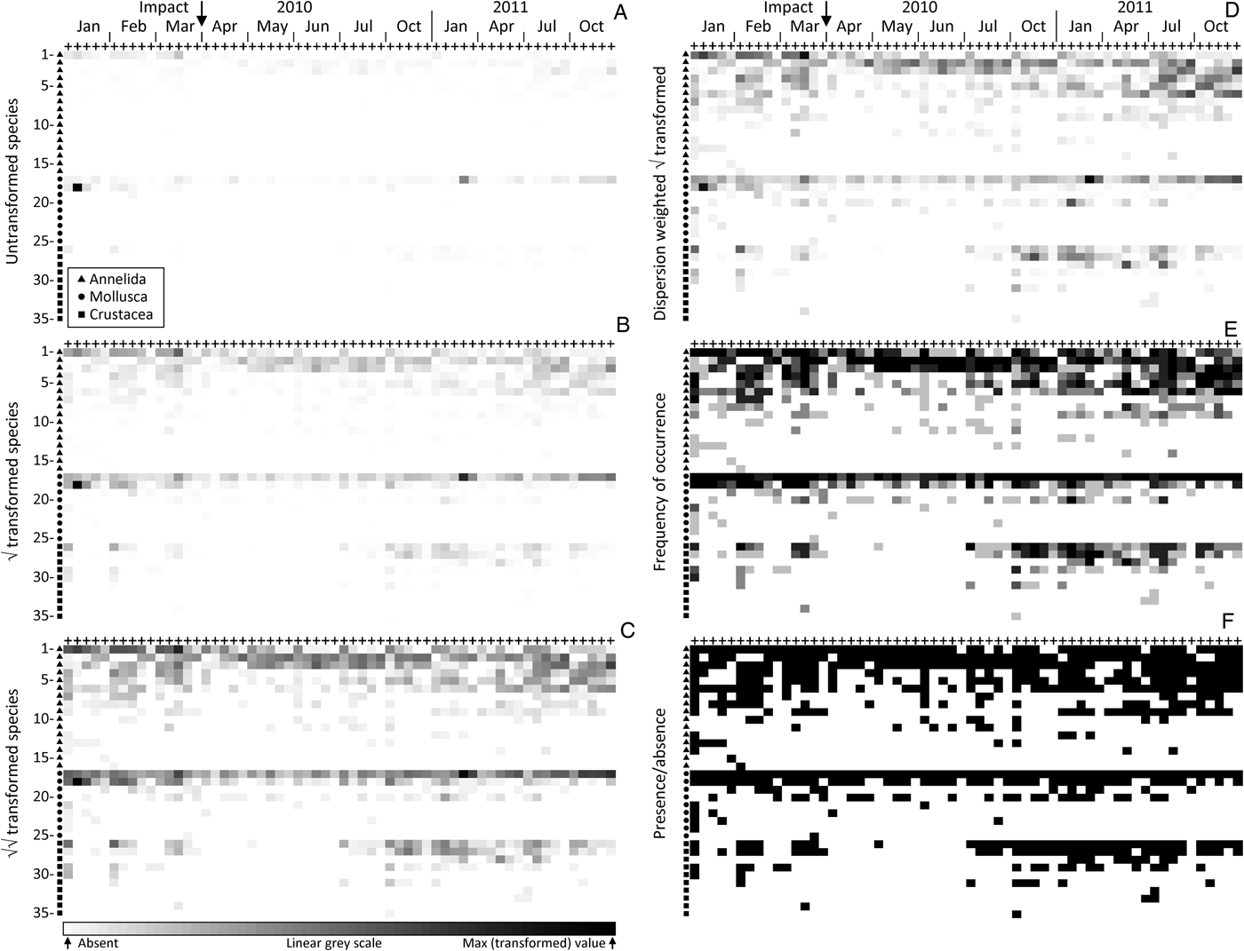
Shade plots for the 60 time-by-location combinations (x axis) and 35 species (y axis) in the order given in Table 1 are shown in Figure 1 (species numbers are hereafter denoted in square brackets). The component plots (A–F) represent different transformations of the species counts from the five replicate grabs, which have then been averaged to the 60 time–location levels. In the absence of any transformation (Figure 1A) few species are seen to have the capacity to contribute to the multivariate analysis at all; the plot is a sea of white space! This results from a single mollusc species, Fluviolanatus subtortus [18], with a total count of 9403 individuals at one of the five locations during the first sampling time, January 2010. Its average count per grab (1881) for that location and time is the maximum value in the matrix and therefore represented by the blackest rectangle. Only the counts for another mollusc species, Arthritica semen [17], approach this value, at a total count of 3802 (average 760 per grab) for a different location in January 2011, and an average of 163 per grab over all locations in October 2011. In fact this latter species is nearly ubiquitous, being found in 92% of the replicate grabs over all times and locations (Table 1) but its counts sometimes range down to tens or units (the lowest non-zero value for any species in the averaged matrix must be 0.2), so that these smaller values are dwarfed by the single largest average count in the matrix and are barely evident at all in this plot. That they exist can be seen from the presence/absence shade plot (Figure 1F) where the unbroken black line for A. semen demonstrates its presence in all 60 time–location combinations. About the only other species barely visible on this untransformed shade plot is the dominant annelid (Table 1), Pseudopolydora kempi [1], whose counts in the first three months average 95 individuals per grab.
Upper Swan macrobenthos. Comparative shade plots for averaged samples in 60 combinations of the same five locations at 12 times (x axis), spanning a potential impact between sampling dates March and April 2010. The 35 species (y axis) are ordered identically for all component plots, within the three higher taxa (denoted by different symbols on the y axis), by decreasing total counts across all samples. See Table 1 for species names, listed in the same order. Depth of rectangle shading represents abundances from the (transformed) species-by-samples matrix, on a continuously linear grey-scale from absent (white) to the maximum value in that matrix (black). Transformations shown are: (A) untransformed (values 0, through smallest non-zero 0.2, to maximum 1880); (B) square-root (0, 0.2, 34); (C) fourth-root (0, 0.2, 5.4); (D) dispersion weighting of each species (see text and Table 1) with further square-root transform (0, 0.04, 4.4); (E) frequency of occurrence in five replicate grabs (0, 0.2, 1); (F) presence/absence (0, 1, 1).

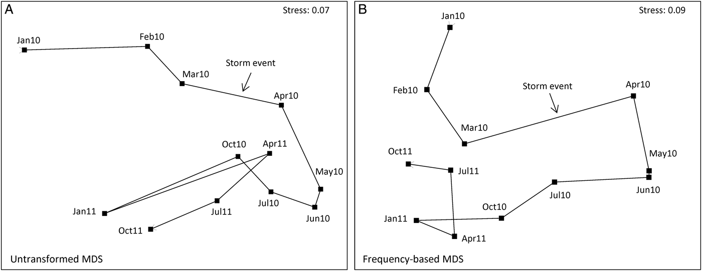
Were a resemblance measure such as Euclidean or Manhattan distance to be calculated on the untransformed data represented by Figure 1A, it could scarcely do other than generate an ordination plot in which the above January 2010 sample would be a complete outlier, with all other samples (barring that from January 2011 referred to above) collapsing into a small region of the ordination. This is because such standard (non-biological) distance measures are dominated by the total count across species for each sample, here a heavily skewed distribution with major outliers. Fortunately, a biologically-based similarity measure such as Bray–Curtis comes partially to the rescue (one of the several reasons for its use) by its inherent standardization of summed absolute differences between pairs of samples (columns) by the sum of the two sample totals. Thus, when there are no large counts in either column the similarities will adjust themselves to the lower abundance scales for each specific pair of samples, and a viable set of similarities may result. The resulting analyses will still largely be dictated, however, by the same two or three dominant species. In the non-metric MDS from Bray–Curtis similarities on samples averaged further over sites, to give the mean assemblage for each of the 12 sampling times (each an average of 25 grabs), it can be seen that the three points to the far left of the ordination (Figure 2A) are precisely the three times (January 2010, January 2011, October 2011) in which F. subtortus and A. semen have their dominant counts. And there is no clear sense from the ordination that this narrowly-based analysis, utilizing mainly just a pair of abundant species, is capturing the a priori structure of most interest, that of a pulse impact from the major storm event of late March 2010, and a possible recovery trajectory for the community some months later.
Upper Swan macrobenthos. Non-metric MDS plots in 2-D, based on Bray–Curtis similarities of assemblages at the 12 time points, from averages of all samples over the five locations, using: (A) untransformed abundances for the five replicate grabs per site and time (cf. Figure 1A); (B) presence/absence at the replicate level, leading to frequency of occurrence of each species in the 25 samples for each time point (cf. Figure 1E).
It is immediately apparent from the shade plot for square-root transformed counts (Figure 1B) that, though this is a relatively mild transformation, it will bring several further species into the computation of similarities, and therefore lead to a more broadly based view of the community structure. The greater ubiquity of A. semen [17] is now clearly seen, though its presence everywhere is not yet apparent in the similarity computation (some light greys are effectively white), and there is a clear suggestion of lower abundance for this species in the immediate post-storm months, picking up again in the recovery period, i.e. from October 2010 onwards. Fluviolanatus subtortus [18] on the other hand is seen to be a species whose medium to large counts are almost entirely restricted to the first three months. The annelid P. kempi [1] is also a major contributor to the pre-impact community under this transformation, with generally lower counts thereafter, often at only one of the five sites. This latter point would be seen more clearly in an x axis ordered firstly by location, then by time within location: as remarked earlier, multiple shade plots for different natural orderings of the axes can sometimes be informative. In addition, other annelids are now treated with nearly the same importance. Prionospio cirrifera [2] and Desdemona ornata [3] do not display a strong time pattern though have a consistent run of relatively high counts in the months following the storm event. Leitoscoloplos normalis [4], Simplisetia aequisetis [5] and Capitella capitata [6] are seen to make a weaker, but clearer-cut contribution to the community prior to the impact event and during the latter half of the recovery period. However, they apparently disappear between those times, this trend for C. capitata being a good indication that the natural state of the upper Swan Estuary in recent years is that of nutrient-enriched sediments from widespread agricultural run-off (see Wildsmith et al., Reference Wildsmith, Rose, Potter, Warwick and Clarke2011; Tweedley et al., Reference Tweedley, Warwick, Valesini, Platell and Potter2012). A similar pattern of apparent absence during the immediate post-storm period is beginning to be established for Paracorophium excavatum [26] and Grandidierella propodentata [27], the two most abundant and frequently occurring crustaceans (Table 1).
The more severe fourth-root transformation further reduces the differential between the largest and smallest non-zero values in the matrix (see legend to Figure 1) from a ratio of 9400 for the untransformed plot, through 170 for the square-root to 27 for the fourth-root. This reduction is the purpose of transformation, of course. It allows a species with a single individual in only one of the replicate grabs (in this case always returning a value of 0.2 in the transformed, then averaged matrix, whatever the power transformation) to be put on a footing which, though not comparable with the largest abundance in the fourth-root averaged matrix (5.4), is no longer vanishingly small in comparison, as it is for square-root or untransformed data. The rarest species will therefore enter into some of the pairwise similarity calculations, at least in small measure. This is visually well-captured in the corresponding shade plot (Figure 1C), where a grey-scale gradation of a factor of only 27 makes many more presences observable (though not quite the very least abundant). Further annelid taxa, Boccardiella limnicola [7], Oligochaeta spp. [8] and Marphysa sanguinea [9] now contribute—sporadically and with less certainty—to somewhat higher abundances and greater observable presence outside the immediate post-event period. Notably also, the pattern of disappearance of crustaceans during that time becomes more accentuated, though values for the dominant P. excavatum [26] and G. propodentata [27] are still substantially lower than those for the dominant molluscs, so the former still play a subsidiary role to the latter in resemblance calculations. For the dominant molluscs, in particular A. semen [17], the compression of the measurement scale from a severe transformation now down-weights its contribution to differentiating the immediate post-event period from earlier and later times, a counterbalance to the potentially greater discrimination achieved by ‘inviting more species to the party’.
Indeed, it is now apparent from Figure 1C that A. semen is likely to be present at all times and locations, and this is confirmed by the ultimate in severe transformations, namely reduction to purely presence or absence of a species for each of the 60 time-by-location combinations, for which Figure 1F displays a solid black line for that species. At this coarseness of measurement scale, A. semen can therefore make no contribution at all to differentiating the time course, and indeed neither do the two dominant annelid species, Pseudopolydora kempi [1] and Prionospio cirrifera [2], whose small number of absences are scattered randomly across times and locations. One gain in this case is that the wide-scale absence of crustaceans over the post-event period is now brought into sharp relief, and they achieve now as much weight as the initially more dominant annelids and molluscs. The downside is that many other species are also given that weight, including some (such as the fourth dominant mollusc, Arcuatula senhousia [20], and a number of other annelids) whose contributions across a wide and randomly scattered set of samples serve only to diffuse the pattern. Thus, whilst untransformed data can lead to much too high a ratio of largest to smallest non-zero abundance for the subsequent multivariate analysis to be considered properly community-based at all (Figure 1A), too harsh a transformation can threaten anarchy, with its insistence on hoovering up the noise as strongly as the signal (Figure 1F).
Formally, this can be seen here in the global R statistics for the simple one-way ANOSIM test of differences among the ‘before’, ‘after’ and ‘recovery’ periods formulated in the Materials and Methods section (first three months, next four months, then the final five quarterly samples, respectively). Through no transform, square-root, fourth-root and presence/absence, R takes respective values 0.62, 0.83, 0.84 and 0.66. This is a commonly observed pattern for such a transformation sequence, both in ANOSIM tests for categorical factors (Clarke et al., Reference Clarke, Somerfield and Chapman2006b) and in regression-style linking (via the BEST ρ statistic) of community change to environmental drivers (Olsgard et al., Reference Olsgard, Somerfield and Carr1997); it seems almost always to be the intermediate transformations that best capture the driving patterns. The novelty here is the realization that shade plots have the capacity to direct the researcher simply, transparently and sometimes strikingly to the underlying reasons for that.
In many analyses, choices are restricted to something like the above transformation sequence (Clarke & Warwick, 2001), perhaps with the addition of log(1 + x) which is more severe than fourth-root for the larger abundances, at least if x represents genuinely integer counts, so tends to give multivariate test results slightly to the presence/absence side of the fourth-root transformation (e.g. a log transform here gives a global R of 0.81). The addition of the +1 constant is important in retaining a transformed value of zero when x = 0, for shade plots and biological-type similarity calculations such as Bray–Curtis. An aside, but an important and widely underappreciated point, is that if x is non-integral, as in density, biomass or area cover measurements, log(1 + x) can run the gamut from very severe to very mild transformation depending on the order of magnitude of the x values. Thus for x values which happen to be scaled, for example, in the range 0.001 to 0.1 (not unknown for CPUE or density/m3), the series expansion for
 $$x\lt1\colon \log_e \lpar 1 + x\rpar = x - \lpar x^2/2\rpar + \lpar x^3/3\rpar - \cdots$$
shows the log transform to be irrelevant, giving log(1 + x) ≈ x. Scaling x up (by 103, for this example) before taking the log transform is an obvious solution but computed similarities will be a function of the magnitude of the arbitrary rescaling factor, and in such circumstances it might be considered preferable to use a power transformation such as fourth-root, giving Bray–Curtis similarities which are invariant to any global rescaling of all matrix entries.
In the current context however, as a result of the averaging of replicate grabs, another simple and severe transformation is possible, namely averaging the presence/absence information for replicates, to give frequencies of occurrence at each time-by-location combination, on a six-point scale: 0, 0.2, 0.4, 0.6, 0.8, 1. This can be seen as intermediate between a fourth-root transformation and pure presence/absence at the time-by-location level, since it compresses the scale still further to a ratio of 5 for the largest to smallest non-zero values. All presences are now clearly seen (Figure 1E) but are not given the equal weight they are in Figure 1F, so that the ability of low-abundance, sporadically occurring species (‘noise’) to degrade the ‘signal’ is lessened. The pattern of disappearance of the main crustaceans (species [26–31]) during the ‘after’ period appears equally clear to that seen for the fourth-root transform in Figure 1C but is here given as much weight as the main mollusc data (species [17–20]), because actual counts are being ignored. This is counterbalanced by the lack of discrimination of the time periods for the dominant mollusc, Arthritica semen [17], noted in Figure 1F; this species is not present in all replicate grabs, but is very nearly so. There is also a greater emphasis (though still substantially less than for the pure presence/absence case) on randomly scattered values for the least abundant annelid species and the mollusc Arcuatula senhousia [20]. The net result is to make this simpler sampling protocol—requiring only recording of the presence of each species in each grab—nearly as effective as the transformed quantitative data, for assessing community change from the shade plot and in testing among the three periods (ANOSIM global R = 0.79). The MDS plot based on these frequency data is shown in Figure 2B and the trajectory shows the dramatic change between March and April 2010 and the subsequent movement of the community back towards its earlier structure. Broadly similar MDS trajectories result from the use of fourth-root or square-root transformed quantitative data (not shown).
An important implication from the above discussion is that, whilst MDS plots and ANOSIM results may be very comparable across transformations varying in their degree of severity, particularly the mid-range power transforms of square- and fourth-root (and here the frequency-based analysis of Figure 1E), the balance of species responsible for those patterns may change substantially. The key point here is that it is commonly observed that environmental factors which drive patterns in one section of a community matrix, such as in the dominant species, also drive much the same patterns in other sections, such as in the less abundant or even rare species (termed ‘structural redundancy’ in the matrix, Clarke & Warwick, Reference Clarke and Warwick1998). Another example of the same phenomenon is seen in Gray et al. (Reference Gray, Aschan, Carr, Clarke, Green, Pearson, Rosenberg and Warwick1988), viz. MDS plots from counts of each species are often remarkably similar to MDS plots of the biomass of each species, even though SIMPER analyses will demonstrate that the species driving group structures, for example, are entirely different for the two analyses—abundance dominants are often very small-bodied so do not dominate the biomass, with the biomass dominants often being large-bodied species found in small numbers.
The remaining component plot in the first figure concerns the effect dispersion weighting (DW, see Introduction) can have on changing the relative weights given to each species in any subsequent similarity calculation. Species which are highly erratic in their counts over the replicate grabs (they are captured in clumps) are heavily down-weighted by DW in favour of species which are very consistent over replicates (they arrive as individuals). Table 1 shows that F. subtortus has the highest variance to mean ratio in counts over replicates, averaged across the ≤60 time-by-location combinations in which this species occurs ( $\overline{D} \approx 100$). Next highest is the other dominant mollusc, A. semen (
 $\overline{D} \approx 45$). By comparison, the three dominant annelids are down-weighted somewhat less severely ($\overline{D}$ between about 15 and 25), and the two dominant crustaceans down-weighted slightly less severely again. However, having divided each species by its dispersion index value $\overline{D}$, the two molluscs F. subortus [18] and A. semen [17], now joined by the annelid P. kempi [1], are still outlying values in the resulting matrix (shade plot not shown but it is again very sparse and roughly intermediate between Figure 1A and 1B). That is, these three species have consistently large counts over all replicates at one of the 60 time-by-location combinations (a different combination for each). In effect, counting capture of centres of population for these species, rather than counting individuals, removes one of the two reasons for transforming counts (Clarke et al., Reference Clarke, Chapman, Somerfield and Needham2006a)—all species now have the same degree of statistical reliability—but it does not address the issue that some species just have consistently much larger counts than others and will still dominate the ensuing analysis.
A square-root transformation following DW produces a more satisfactory balance of consistently abundant with consistently less abundant species (Figure 1D), whilst scarcely allowing the low abundance and rare species to make the potentially random contribution they might do in a purely presence/absence analysis. This shade plot is seen to be intermediate between the square-root and fourth-root transformed shade plots without DW (Figure 1B and 1C, respectively), though closer to the latter. During the ‘after’ period, the loss of crustaceans and the lower values for the dominant mollusc (A. semen [17]) and some annelid species (L. normalis [4], S. aequisetis [5], C. capitata [6]), which are given more weight by DW because of their relative consistency, is enough to give a large ANOSIM R statistic of 0.84 for the global test of the three time periods. This is now equivalent to the highest value from the routine transformation sequence, for the fourth-root transform (Figure 1C). The implication is clear: using DW to treat each species on its own merit, in terms of statistical reliability, is more theoretically satisfactory than taking a large hammer to the data to squash down the high abundance/high variability species, compressing the less abundant species to a near presence/absence contribution in the process (Clarke et al., Reference Clarke, Chapman, Somerfield and Needham2006a), but it may sometimes still then require fine tuning by a mild transformation before similarity coefficients are calculated. Simple shade plots can be extremely useful in making such judgements. This finding is now examined further for the fish assemblages from south-western Australia, where clumping (schooling of fish of the same species) can be particularly severe.
South-west Australian estuarine fish
The index of association calculated between all pairs of the retained 41 fish species over the 119 sites, based on dispersion-weighted abundances (not further transformed), leads to the hierarchical cluster analysis (Figure 3), as described in the Materials and Methods section. This dendrogram places together species that have common relative abundances across the full set of sites, with the association measure automatically standardizing the abundances for all species so that they each sum to the same number (100%) across all sites. For this (r-mode) cluster analysis therefore, whether a species is initially dispersion-weighted or not becomes irrelevant; it is the pattern of increasing and decreasing values across sites which is being matched for each pair of species. Nevertheless, it is convenient here to indicate, as a divisor to each species name in Figure 3, the average dispersion index $\overline{D}$ for that species, calculated from replicate seines. This is because that ordering of species, with its associated dendrogram, is adopted for all the component shade plots in Figure 4, where the dispersion weighting does, of course, have a substantial impact on the species values there represented. The down-weighting of counts for schooling species in the subsequent multivariate analyses range from a maximum factor of 471 for Hyperlophus vittatus, through about 170 for Spratelloides robustus and Atherinosoma elongata, around 90 for Atherinomorus ogilbyi and Leptatherina wallacei, about 40–70 for Leptatherina presbyteroides, Craterocephalus mugiloides and Craterocephalus pauciradiatus, and down to single figures for half the remaining species. The latter include several (with no divisor indicated) for which the hypothesis of independent arrivals of individuals into the sample (Poisson counts) cannot be rejected by a permutation test (Clarke et al., Reference Clarke, Chapman, Somerfield and Needham2006a).
South-western Australian fish. Dendrogram from hierarchical group-average (r-mode) clustering of 41 species, based on Whittaker's index of association among pairs of species (i.e. Bray–Curtis on species-standardized data). The resemblance calculations use dispersion-weighted abundances for each species from replicate seine net sampling, seasonally-averaging them within 119 sites spread across five estuaries. The DW divisor which down-weights each species is indicated (/$\overline{D}$) when >1, and this listing determines the species ordering in the shade plots of Figure 4.

South-western Australian fish. Shade plots for 119 sites over five estuaries (x axis): Peel–Harvey, Swan–Canning, Wellstead, Wilson and Broke, from abundances after dispersion weighting of 41 species, clustered and ordered as in Figure 3 (y axis). Estuaries, and sites within estuaries, are ordered left to right in decreasing (time-averaged) values of a roughly equally-weighted combination of salinity, water temperature and dissolved oxygen concentration at those sites (PC1 of normalized measurements). As in Figure 1, rectangle shading is on a linear grey scale from absence (white) to the maximum matrix entry (black), for increasingly severe transformations: (A) abundances after DW but not further transformed; (B) DW then square-root; (C) DW then fourth-root; (D) presence/absence data (for which prior DW is irrelevant).

However, even after this major selective down-weighting of some of the most erratic counts, the shade plot of the dispersion-weighted but untransformed data matrix (Figure 4A) is still largely dominated by two of the species subject to the greatest down-weighting, A. elongata and L. wallacei. Along with a third species, Pseudogobius olorum (all three of which are clustered together in the top part of the dendrogram of Figure 3), they are clearly seen to be mainly responsible for characterizing the assemblage in the Wellstead Estuary, for example. In contrast, Figure 4A shows that H. vittatus, the only other species even visible on a simple shade plot of the untransformed data without DW (not shown), no longer plays a role in determining similarities. Dispersion weighting has thus succeeded well in removing the emphasis that this species would have continued to exert under conventional transformation but which came from a few, very large agglomerations of individuals sporadically distributed among some sites in the Peel–Harvey Estuary (with counts in the thousands or even, in one seine net sample, in the tens of thousands). However, the other two initially dominant species, A. elongata and L. wallacei, with counts in the high hundreds or low thousands in many net samples, can be found consistently with such high numbers across all replicates at a wide spread of sites. Even after a down-weighting by two orders of magnitude they return consistent values in the tens over a wide spread of sites, and Figure 4A shows that they still play a dominant role in defining similarities.
A square-root transformation of the (dispersion-weighted) matrix, therefore, looks desirable to better balance consistently higher with consistently lower values, and bring more species into play in characterizing the assemblage structure. That this is effective is seen in the shade plot of Figure 4B; the previously mentioned block of three species near the top of the list which typify the Wellstead Estuary are joined by a fourth in the same cluster, Afurcagobius suppositus, and two more species towards the middle of the list, Favonigobius lateralis (a more or less ubiquitous species) and L. presbyteroides, in characterizing the Wilson and Broke Inlets. In contrast, for the Peel–Harvey and Swan–Canning Estuaries a large number of other species come into play, with comparable magnitudes to the previously dominant species near the head of the list.
A great deal more interpretation of the patterns of particular species, or groups of species, across the differing estuaries, could be drawn from a shade plot such as Figure 4B. However, for our current illustrative purposes, we concentrate only on two interesting features: the extent to which the patterns observed in the shade plots of Figure 4, under different transformations, help to interpret the multivariate ordination plots shown in Figure 5, and the extent to which choice of ordering of sites on the shade plot can inform interpretation of observed continuous change within an estuary.
South-western Australian fish. (A–D) Non-metric 2-D MDS plots of assemblages at the 119 sites from five estuaries, using the time-averaged abundance matrices visualized in the shade plots of Figure 4A–D, respectively, and based on Bray–Curtis similarities among sites.

The corresponding MDS ordination to Figure 4A, based on Bray–Curtis similarities from the dispersion-weighted but untransformed data, is seen in Figure 5A. Notable is the high stress, an indication that the ordination is not a function only of the dominant two or three species after DW, as would have been the case if based on data not subject to DW or transformation; a number of other species do contribute something here. That high stress, however, is also an indication that the primary structure driving this pattern, largely the among estuary differences, is not clear-cut; the ‘noise to signal’ ratio is quite high. Note the clear separation of four of the Swan–Canning Estuary sites from the other 20 sites in Figure 5A. Though care must be taken in interpreting 2-D MDS plots with a stress as high as 0.17, the shade plots are helpful in visualizing the reasons for such a separation. These four sites are at the right-hand side of the Swan–Canning Estuary block in Figure 4, having the lowest average values of salinity, water temperature and dissolved oxygen concentration for that estuary (noting that, within estuaries, the sites have been ordered by decreasing values of the first PC of these normalized variables, see Materials and Methods). In terms of visibility at this untransformed level they share some of the dominant species that characterize Wellstead, Wilson and Broke sites, and contain some species at the bottom of the dendrogram list which they share with other Swan–Canning sites, but are largely missing a raft of species in the middle of the dendrogram which characterize the Peel–Harvey Estuary and the rest of the Swan–Canning sites. Their separation on the MDS plot is therefore not simply due to the inadequacy (high stress) of representation in low-dimensional space of sample relationships in 41 dimensions.
The MDS plot (Figure 5B) which is based on the dispersion-weighted and square-root transformed data of Figure 4B has lower stress because there is now a clearer structure to the estuary differences, with the greater separation in the MDS of Peel–Harvey and Swan–Canning sites from Wellstead, Wilson and Broke samples being mirrored in the corresponding shade plot, largely due to the visibly greater contributions from a much richer species set in the former two estuaries, as noted above. The division into two estuary groups continues to widen for the remaining two transformations, fourth-root and presence/absence (Figure 5C and 5D, the prior DW becoming irrelevant in the latter case). This division now owes little to the dominant species noted in Figure 4A and 4B, characterizing the Wellstead, Wilson and Broke sites, as they are seen (Figure 4C and 4D) to be more or less ubiquitous, and thus make an increasingly ignorable contribution to similarities underlying the MDS plots of Figure 5C and 5D. It is the continuation of the trend for ever greater prominence of the larger number of species found in the Peel–Harvey and Swan–Canning Estuaries which drives the increasing separation of the two estuary groups in the later MDS plots and leads to a further decrease in their stress values. Note that this is somewhat unusual: Clarke & Warwick (Reference Clarke and Warwick2001) comment that increasing the severity of a transformation, and thus bringing more species into play, will automatically place the among-sample relationships into higher-dimensional species space, and typically make it more difficult to obtain an accurate (low stress) 2-D ordination. This is interestingly counteracted here by the species entering under heavier transformation imposing a much stronger ‘signal to noise’ ratio on the pattern; these low-abundance species all largely have a correlated pattern of presence in the first two estuaries and absence for the last three, so do not greatly increase the true dimensionality of the larger species set. It must also be appreciated that the initial reduction of the species set to the 41 ‘most important’ (see Materials and Methods) is also a factor here. If the full set of 97 estuarine fish species had been retained, they would have added back a greater degree of high-dimensional random ‘noise’ to the presence/absence analysis.
A second notable feature of the shade plots for Broke Inlet is the apparent steady decline in numbers for virtually all six of the characterizing species identified earlier (A. elongata, L. wallacei, P. olorum, A. suppositus, F. lateralis and L. presbyteroides) with decreasing average salinity, water temperature and dissolved oxygen concentration measurements, namely the left to right ordering of sites within an estuary imposed on the x axis of the shade plots. This is seen most clearly for the square-root transformed data (Figure 4B) and is also suggested by the apparently linear structure of the Broke points on the corresponding ordination plot (Figure 5B). It is visually demonstrated that this linearity is indeed linked directly to the first principal component (PC1) of these three water quality measurements by a bubble plot for the MDS ordination on dispersion weighted and square-root transformed data (Figure 6), in which bubble size represents PC1 values. The relationship for Broke is clear, and the relevant formal RELATE test (see Materials and Methods), matching dissimilarities for Broke site assemblages with corresponding (Euclidean) distances among univariate PC1 values, gives statistics of ρ = 0.39, 0.44, 0.42 and 0.28, respectively, for the four transformations of Figure 4 (there are sufficiently many sites to make all of these values significantly different from zero, borderline values only being obtained for ρ values below 0.2). The combined 2-way RELATE test which looks at this relationship of site assemblages to the water quality PC1 variable separately within estuaries but over all five simultaneously (then averages and tests the resulting $\bar{\rho}$), results in statistics $\bar{\rho}$ = 0.33, 0.36, 0.33 and 0.20, respectively, for the four transformations. As might be expected from Figure 6, there is some relationship to PC1 for estuary sites other than Broke (with the exception of Wellstead) but the generally weaker links drag down the average $\bar{\rho}$ values for this two-way version of the test.
South-western Australian fish. Bubble plot for the assemblage MDS of Figure 5B (abundances under DW and square-root transform) in which circles of increasing size are placed on the 119 site positions in proportion to increasing value of the first principal component of the (normalized) water quality variables. Estuaries are indicated by differing grey shades for the bubbles.

What is clear however, is that the mild transformation of a square-root, following DW, strikes the best balance in preserving the relevant information here. Too severe a transform risks throwing away the informative (and now reliable data, following DW) that is present in quantitative counts; no transform at all risks the analysis still being over-dominated by one or two species which have consistently high counts over replicates. Generality of this conclusion cannot be claimed on the evidence of just two examples, but what is argued here is that a few simple shade plots should be enough to make it clear when a transformation has been too extreme, in either direction, whether that transformation is on the original data or on its dispersion-weighted form. Amidst all the very necessary sophistication of multivariate hypothesis testing and low-dimensional summaries of complex high-dimensional structures, safeguarding the user from interpreting patterns for which there is no statistical support, it is never a bad idea to keep the data itself firmly in view, and shade plots do precisely that!
Note also how important it was to the interpretation of the MDS bubble plot for Broke samples in Figure 6 that the shade plot x axis be ordered according to the pattern in the environmental variables, and the visual assistance provided by grouping species on the y axis according to their mutual associations. Several different orderings of the x axis could be envisaged, depending on the hypotheses of interest, but in a case such as this where the ordering is determined by an exogenous variable (or combination of variables), and the species axis is ordered on internal grounds, independently of that information, a shade plot can be an insightful way of spotting not just a link between the two axes but also the reasons for that relationship.
CONCLUDING REMARKS
Simple shade plot comparisons such as in Figures 1 and 4 can be extraordinarily powerful in informing the user about the effect that different choices for data pre-treatment (dispersion weighting, transformation, standardization, etc.) can have on the relative weighting given to different species in subsequent multivariate tests, clustering and ordination displays of the samples. It should be re-emphasized, however, that the idea is not to choose a pre-treatment combination that best demonstrates one's preconceptions of what message the data should contain! There is always a danger of selection bias when faced with multiple choices in a situation where precisely the same data are used to make those choices as are subsequently used to test the hypotheses of interest. This is seen at its most extreme when ANOVA is performed separately on each of a large number of species, resulting in just a small handful of ‘significant’ species, which are then pulled out for further examination. Selection bias in that case can be extreme and dangerously misleading. Here, the number of choices between transformations is typically rather limited and Type I errors can only be compromised to a limited degree, in borderline cases, by selecting the ‘best’ transformation. Nonetheless, for that reason, no emphasis has been given to p values for the ANOSIM or RELATE tests in this paper, though all were overwhelmingly significant in conventional terms. Rather, the ideal is that shade plots can play a useful role in deciding which transformations and/or dispersion weighting would be best to adopt for routine long-term use with particular faunal groups, study areas, sampling methods and sizes, and for the nature of the hypotheses being examined. In particular, it might well identify certain extreme choices (e.g. no transform, reduction to presence/absence) as unlikely to be beneficial for the long-term goals of the study.
In addition, when multivariate hypothesis tests are significant and justify closer examination of the species patterns that such tests have demonstrated, the use of shade plots a posteriori can also be extraordinarily powerful, as Figures 1 and 4 amply demonstrate. They have the capacity not only to identify common patterns in groups of taxa which appear to be determining sample group structures (as an alternative or an adjunct to categorical, similarity-based tools such as SIMPER, Clarke, Reference Clarke1993) but also, by suitable re-ordering of shade plot axes, to interpret continuous multivariate assemblage change at the level of individual species.
ACKNOWLEDGEMENTS
We thank the referees for their positive and helpful comments. We also thank Michelle Wildsmith, Mathew Hourston, Natasha Coen, Christopher Hallett, Thea Linke, Alan Cottingham, Amanda Buckland, Ben French and Lauren Veale for assistance in the collection and processing of the samples underlying these data. Thanks are due in particular to Ray Gorley of PRIMER-E, Plymouth for his coding of these developments in the PRIMER software. K.R.C. acknowledges his Honorary Fellowship position at the Plymouth Marine Laboratory, UK, his adjunct Professorial position within the Centre for Fish and Fisheries Research at Murdoch University, Western Australia and expresses his gratitude to Professor Ian C. Potter (Murdoch University) for facilitating fruitful, long-term collaborations.
FINANCIAL SUPPORT
The Swan River Trust, the Australian Fisheries Research and Development Corporation, the Department of Environment and Conservation and Murdoch University are gratefully acknowledged for funding the data collection used in the illustrative examples of this paper.